Modeling coupled electrochemical and mechanical behavior of soft ionic materials and ionotronic devices

Abstract

Recently there has been an increase in demand for soft and biocompatible electronic devices capable of withstanding large stretch. Ionically conductive polymers present a promising class of soft materials for these emerging applications due to their ability to realize charge transport across the polymer network, while preserving the desired mechanical and chemical features. As opposed to electron transfer in traditional electrical conductors, the charge transport across these polymers is achieved through ion migration. When such materials are used in combination with electrical systems, they are known as ionotronic devices. The ability to simulate device performance based on its material composition and geometry would accelerate and improve ionotronic device design. The main challenge in developing reliable simulation capabilities for ionically conductive polymers is the complex and coupled electro-chemo-mechanical behavior. In this work we address this challenge by introducing a multiphysics framework incorporating the coupled effects of ion transport, electric fields and large deformation. The utility of the developed multiphysics model is showcased by simulating representative ion transport problems and the operation of soft ionotronic devices.

1 Introduction

Soft and deformable ionic conductors, such as hydrogels and polyelectrolytes, present a promising class of materials for integration into soft circuits and ionotronic devices. Traditional electric circuits are mainly composed of hard and rigid electrically conductive materials, and are therefore ill suited for applications requiring large deformation. Flexible conductors fall into one of four categories: (i) hard conductors that flex by bending/unbending (Kim et al., 2007; Lee et al., 2012; Song et al., 2014), (ii) liquid metal encapsulated within a soft elastomer matrix (Markvicka et al., 2018; Yan et al., 2019), (iii) electrically conducting polymers (Rivers et al., 2002; Liu et al., 2018), and (iv) ionically conductive materials (Chen et al., 2014; Shi et al., 2018). Soft ionically conducting materials typically consist of polymer networks with mobile ionic groups (e.g., dissociated salts); charge transport across the network occurs by motion of these ions. These soft ionically conducting materials are promising because of environmental responsivity, intrinsically large strain to failure, tunability, and biocompatiblity.

The applications of soft ionically conductive polymers are vast, from healthcare and soft robotics to sensors (Kim and Tadokoro, 2007; Rus and Tolley, 2015; Lacour et al., 2016; Yang and Suo, 2018). Soft ionically conductive polymers are utilized in design of soft circuits, where they are employed as soft cables (Yang et al., 2015; Odent et al., 2017), diodes (Cayre et al., 2007; Gabrielsson et al., 2012; Wang et al., 2019) and transistors (Tybrandt et al., 2010; Shin et al., 2014). They also find application in soft actuators, allowing for design of artificial muscles (Jung et al., 2010; Han et al., 2018; Morales et al., 2014) and biomimetic robots (Yeom and Oh, 2009; Li et al., 2017). Implementing these materials as sensors in soft robotics helps maintain the desired mechanical properties as opposed to more traditional rigid sensors (Sun et al., 2014; Robinson et al., 2015; Liu et al., 2020; Wang et al., 2021). Moreover, energy harvesting devices based on soft ionic conductors, such as the ones published by Aureli et al. (2009); Tiwari and Kim (2010); Hou et al. (2017); Zhou et al. (2017), and Kim et al. (2020), allow for conversion of mechanical deformation into electric potential and current. In energy conversion technologies, such as batteries and fuel cells, these materials are typically referred to as polymer electrolytes or polymer electrolyte membranes (cf. e.g., Wan et al., 2019; Chen et al., 2017; Banerjee and Curtin, 2004). In this context they provide a mechanical barrier in addition to the ionic conductivity and electrical insulation necessary in a liquid electrolyte (solution with dissociated ions).

Thorough characterization of the electrochemical response greatly faciliates successful implemention of soft polymers into ionotronic devices. Electrochemical impedance spectroscopy (EIS) is a common experimental method that involves applying a small electric potential perturbation across the specimen while measuring the current signal. The perturbation is typically applied as a sinusoidal voltage signal with a constant and small amplitude, to ensure the material response is within the linear regime. The EIS data is then analyzed by comparing the voltage and current waves, as shown in Figure 1a. The experimental data is commonly presented as Bode plots, with the impedance magnitude $|$Z$|$ computed as the voltage-to-current amplitude ratio $|$V$|\,/\,|$I$|$, and plotted together with the phase shift angle $\delta$. Overall, EIS provides information about the mechanisms of charge conduction, and can be used to evaluate the performance of ionic materials and ionotronic devices.

a)	b)

Figure 1: Fundamentals of EIS and underlying physics. a) EIS involves applying a small amplitude sinusoidal voltage V and measuring the current signal I. The two sinusoidal waves are then compared to obtain the impedance magnitude as $|$V$|/|$I$|$, and phase shift angle $\delta$. Here, $\alpha$ denotes the frequency dependent conversion factor given in units s$/^{\circ}$. b) A snapshot of the ionic conductor subjected to an external AC voltage source V. The electric field is established and the mobile ions migrate towards the oppositely charged electrode. At the polymer/electrode interface the ions screen the charges on the electrode surface, thus forming a diffuse double layer. The Stern layer represents the first ion layer adsorbed onto the surface, denoted with gray shading (note that we do not explicitly model this layer).

Despite the rapid increase in the number of potential applications, there is a lack of overarching design tools, hindering the further advance of ionotronic technology. The main challenge in developing reliable simulation capabilities for ionotronics is the coupled electro-chemo-mechanical behavior. The most common approach for evaluating ionotronic device and material performance is fitting EIS data to equivalent circuit models. While these models provide information on the response of systems within electrical circuits, there is minimal insight into the relations among the material, device structure, charge transport mechanisms, and observed electrochemical response. EIS data can be fitted to many different equivalent circuits, and understanding the mechanisms driving the electrochemical phenomena is required for selecting an accurate circuit model. Moreover, many soft ionic conductors are expected to operate under large mechanical deformation – another feature not captured by equivalent circuit models.

Aside from the equivalent circuit modeling, there are many continuum-level models that capture the electrochemical behavior of ionotronic materials. The seminal works of Walther Nernst (Nernst, 1888) and Max Planck (Planck, 1890) capture the transport of charged species in an electrolyte. The introduced modification to the conservation of mass included the influence of electric fields on ionic diffusion – a relation commonly referred to as the Nernst-Planck equation. Additionally, the charge concentration alters the electric field; and the relation between the two is given by one of the four Maxwell equations – Gauss’s law (Gauss, 1877), commonly represented in the form of Poisson’s equation (Poisson, 1826). These coupled effects of charge transport and electric potential are captured by the Poisson-Nernst-Planck relations. Building upon the seminal theories, there have been many notable works capturing charge transport in the presence of electric fields (cf.,e.g., Buck, 1969; Mizushina, 1971; Kornyshev and Vorotyntsev, 1981; Corry et al., 2000; Gillespie et al., 2002; Bazant et al., 2004). Such models allow for computational investigation of electrochemical systems and open the door for analysis of advanced ionotronic devices through numerical simulations on intricate geometries and under complex boundary conditions. Towards this goal, different numerical methods have been proposed for solving the electrochemically coupled problems, including the finite difference method (Brumleve and Buck, 1978; Flavell et al., 2014; Liu and Wang, 2014), finite volume method (Lopreore et al., 2008), and finite element method (Lu et al., 2010; Eisenberg et al., 2011; Paz-García et al., 2011).

The coupling between the electrochemical processes and large mechanical deformation in polyelectrolytes has been modeled previously in the context of environmentally responsive ionic gels and ionic electromechanical transducers. In current literature on electrochemically and mechanically coupled response of environmentally responsive polymers, there are various models accounting for the ionic-driven swelling of polymer gels (cf., e.g., Doi et al., 1992; De Gennes et al., 2000; Wallmersperger et al., 2004; Keller et al., 2011; Drozdov and deClaville Christiansen, 2015; Leichsenring and Wallmersperger, 2017; Zhang et al., 2020; Narayan and Anand, 2022). Recent years also saw notable efforts towards developing multiphysics framework for coupled electrochemistry and mechanics of soft ionic actuators, with most authors focusing on the mechanical response of ionic polymer-metal composites under external electric fields (cf., e.g., Nemat-Nasser, 2002; Toi and Kang, 2005; Nardinocchi et al., 2011; Rossi et al., 2018; Narayan et al., 2021). In addition, similar models have been applied to investigate the perturbation in electrochemical behavior in response to an applied mechanical deformation in sensor-like systems (cf., e.g., Ganser et al., 2019). To complement modeling efforts, the numerical approach laid out by Narayan and Anand (2022) allows for solving the coupled set of electro-chemo-mechanical equations in three-dimensional space under large mechanical deformation. Nonetheless, in current state of the art there is a lack of robust computational capabilities for the influence of multiple mobile ionic species, charged polymeric backbones and large mechanical deformation on ionotronic material and device performance. While out of scope of this research, we also note that literature on modeling of energy storage devices, such as batteries, provides ample electro-chemo-mechanical models. However, the coupled electrochemical and mechanical models developed for batteries are usually focusing on the swelling-induced deformation and electrochemical reactions (cf. e.g., Golmon et al., 2009; Bucci et al., 2014; Rejovitzky et al., 2015; Sauerteig et al., 2018).

To bridge the gap between the increasing demand for soft ionotronic devices and lack of computational tools, in this work, we introduce a continuum-level multiphysics framework and a constitutive model incorporating the coupled effects of electric field, ion transport, and large mechanical deformation on the overall behavior of soft ionotronic materials and devices. We account for the influence of both neutral and charged polymeric backbones, along with the diffusion of multiple ionic species. Our modeling effort is aimed at simulating the electrochemical characterization of soft ionic conductors, along with the operation of ionotronic devices. The usefulness of such a computational tool is twofold: (i) it provides the guidance for modifying the polymer structure towards target electrochemical properties and (ii) it allows for design evaluation of devices through finite element analysis. In our first step towards this goal, we numerically implement the electrochemical framework (i.e., the framework in the absence of mechanical deformation) as a 1D custom finite element code in Matlab. We showcase the reliability of our computational approach by comparison against analytical solutions and EIS data. Then, we include the effects of large mechanical deformation and implement the framework as a user element (UEL) subroutine in Abaqus/Standard. We demonstrate the potential of our numerical tool to understand and design ionotronic systems by simulating the operation of devices found in literature. Accordingly, the remainder of this paper is organized as follows: in Section 2 we develop a continuum-level thermodynamic framework and a constitutive model; in Section 3 we present numerical simulation results; in Section 4 we provide concluding remarks.

2 Multiphysics model

In this section we present a framework and constitutive model for electro-chemo-mechanics of ionically conducting polymers. To facilitate understanding, we start with an overview of the underlying physics, including typical transport mechanisms.

2.1 Overview of the governing physics

Polymeric materials consist of mutually entangled or chemically cross-linked polymer chains which form a polymer network. Ionically conductive polymers contain mobile charged species, i.e. ions. Subjecting these materials to an electric field causes the mobile ions to migrate towards the oppositely charged electrode. At the polymer/electrode interface, ions screen charge at the electrode surface, thus forming a diffuse double layer, as shown in Figure 1b. In this study we assume there is no charge transfer across the electrode/polymer interface, which is analogous to saying we have blocking electrodes. The layer of ions at the interface is known as the Stern layer and its thickness is on the order of angstroms. A common way to quantify the distance over which mobile ions screen charge at the electrode is by computing the Debye length, which is found assuming a Boltzmann distribution for the concentration of charges:

$$\lambda_{D}=\sqrt{\frac{\varepsilon_{r}\varepsilon_{0}RT}{\left(eN_{a}\right)^{2}c^{E}}}\,,$$ (1)

where $\varepsilon_{r}$ is the relative permittivity, $\varepsilon_{0}$ is the dielectric permittivity of vacuum, $R$ is the universal gas constant, $T$ is absolute temperature, $e$ is the elementary charge, and $N_{a}$ is Avogadro’s number. The average concentration of charged species in the electrolyte is obtained as $c^{E}=\sum\left(z^{(i)}\right)^{2}c^{(i)}_{0}\,$, where $z^{(i)}$ denotes the charge and $c^{(i)}_{0}$ the initial concentration of $i$-th mobile ionic species.

2.1.1 Polymer backbone charge

The polymer chains in the network can themselves be either neutral or charged. The degree of charge often depends on pH of the environment, i.e., association/dissociation chemical reactions might occur on groups tethered to the polymer backbone, changing both the degree of fixed charge and concentration of mobile ions. For example, at high pH, mobile protons (H⁺) can easily dissociate from carboxyl groups RCOOH, leaving the negative carboxylate RCOO^- tethered to the backbone ($\textrm{R}\textrm{COOH}\rightleftharpoons\textrm{R}\textrm{COO}^{-}+\textrm{H}^{+}$). Backbones with these negatively charged groups are termed anionic backbones, and the materials are called polyanions or polyanionic. On the other hand, at low pH, the hydrogen can associate with certain functional groups, such as a neutral amino group RNH₂, yielding a positively charged and tethered RNH${}_{3}^{+}$ ($\textrm{R}\textrm{NH}_{2}+\textrm{H}^{+}\rightleftharpoons\textrm{R}\textrm{NH}_{3}^{+}$). The positively charged backbones are termed cationic backbones, and the materials are called polycations or polycationic.

2.1.2 Charge transport mechanisms

There are four major mechanisms for achieving charge transport in ionically conductive polymers; and the effective diffusivity of mobile ions depends on the particular mechanisms dominating the charge transport:

1. Diffusion through an electrolyte is dominant in swollen polymer networks, such as hydrogels, where transport of dissolved and dissociated salts is almost unaffected by the highly hydrated polymer network. The diffusion values are typically $10^{-9}$m²/s plus or minus an order of magnitude. (Lobo et al., 2001; Wu et al., 2009; Schuszter et al., 2017)

2. “Hopping” occurs along the charged functional groups tethered to the backbone of nearly dry and solvent-free polymers. The diffusion coefficients for this regime vary drastically based on the material and processing (e.g. $\sim 10^{-11}\,$m²/s (Choi et al., 2005), $\sim 10^{-12}\,$m²/s (Ochi et al., 2009), $\sim 7\cdot 10^{-15}\,$m²/s (Kim et al., 2020)).

3. The Grotthuss mechanism (transport by hopping along water molecules) is dominant in hydrated proton exchange membranes (PEM), and can be also found in anion exchange membranes (AEM) (cf., e.g., Miyake and Rolandi, 2015). At a continuum scale, this process yields a relatively high diffusion coefficient, up to $\approx 7\cdot 10^{-9}\,$m²/s (Cukierman, 2006; Agmon, 1995; Paddison and Paul, 2002; Choi et al., 2005).

4. Vehicular or en masse transport involves migration of fully solvated ions together with the solvent, i.e., using solvent molecules as a vehicle for transport. The resulting diffusion coefficients are $\approx 2\cdot 10^{-9}\,$m²/s (Agmon, 1995; Li et al., 2001; Choi et al., 2005).

In our continuum-level modeling approach we are not explicitly modeling the above mentioned micromechanics of charge transport. However, we use these as guidelines for selecting a reasonable diffusion coefficient value for each material in our simulations.

It is worth noting that ions diffuse significantly faster than water in the presence of an electric field. Consequently, the change in water content is negligible for the boundary conditions and timescales under consideration here. We therefore assume the hydration level uniform and constant except when directly coupled to ion motion. In addition, we consider pH to affect only the initial charge of the polymer chains and the electrolyte strength, while neglecting any pH driven swelling. We also choose to neglect thermal effects in this manuscript since they will be negligible in the devices we examine.

2.2 Thermodynamic framework

We commence the modeling procedure by introducing the useful kinematic relations, and consider a body $\mathcal{B}_{\textrm{\tiny R}}$ in its referential configuration undergoing a motion $\boldsymbol{\chi}$ to its spatial (i.e., deformed) configuration $\mathcal{B}$. The deformation gradient and velocity are then given by

$${\bf F}=\nabla\boldsymbol{\chi}\quad\textrm{and}\quad{\bf v}=\dot{\boldsymbol{\chi}}$$ (2)

respectively, along with the volumetric deformation $J=\det{\bf F}$. In addition to the mechanical deformation, the presence of ionic species induces deformation of the polymer network. Therefore, we make use of an approach commonly found in gel mechanics literature (cf., e.g., Hong et al., 2008; Chester and Anand, 2010), and decompose the deformation gradient into a mechanical and swelling part

$${\bf F}={\bf F}^{m}{\bf F}^{s}\,,$$ (3)

where ${\bf F}^{m}$ and ${\bf F}^{s}$ are the mechanical and swelling components of the deformation gradient respectively. The volumetric deformation can then be decomposed into

$$J=J^{m}J^{s},$$ (4)

where $J^{m}$ and $J^{s}$ represent the mechanical and swelling volume change respectively. We assume the change in volume results directly from the change in mobile species concentration, with corresponding volumetric swelling in the form

$$J^{s}=\det{\bf F}^{s}=1+\sum_{i}\Omega^{(i)}\left(c_{\textrm{\tiny R}}^{(i)}-c_{\textrm{\tiny R}0}^{(i)}\right)\,,$$ (5)

where $\Omega^{(i)}$, $c_{\textrm{\tiny R}}^{(i)}$, and $c_{\textrm{\tiny R}0}^{(i)}$ are the molar volume, current concentration and initial concentration of the $i$-th mobile ionic species in the referential configuration, respectively.

The right Cauchy-Green tensor is given by

$${\bf C}={\bf F}^{\,{\mskip-2.0mu\scriptscriptstyle\top}}{\bf F}\,={\bf C}^{m}{\bf C}^{s},$$ (6)

where ${\bf C}^{m}$ and ${\bf C}^{s}$ are the mechanical and swelling part of the right Cauchy-Green tensor, respectively. In addition, the left Cauchy-Green tensor is given by

$${\bf B}={\bf F}{\bf F}^{\,{\mskip-2.0mu\scriptscriptstyle\top}}\,.$$ (7)

Next, to capture the multiphysics behavior of soft ionic conductors, we assume the material is affected by (i) the electric field, (ii) the balance of ionic species, and (iii) mechanical stress. As in much of the previous literature on electrically responsive polymers (cf., eg. Wang et al., 2016; Rossi et al., 2018; Narayan et al., 2021), we choose the form of Gauss’s law that gives the relation between the concentration of charged species and the electric displacement in the referential configuration ${\bf d}_{\textrm{\tiny R}}$:

$$eN_{a}\left(\sum_{i}\left(z^{(i)}c^{(i)}_{\textrm{\tiny R}}\right)+z^{(\textrm{fix})}c^{(\textrm{fix})}_{\textrm{\tiny R}}\right)=\hbox{{Div}}\mskip 2.0mu\,{\bf d}_{\textrm{\tiny R}}\,,$$ (8)

where $z^{(i)}$ denotes the charge number of $i$-th mobile species, and $z^{\textrm{(fix)}}$ and $c_{\textrm{\tiny R}}^{\textrm{(fix)}}$ the charge number and concentration of chemical groups tethered to the polymer matrix, and consequently fixed in position, in the reference configuration. We also introduce the net charge density in the spatial configuration as

$$\rho=\sum_{i}\left(z^{(i)}c^{(i)}\right)+z^{(\textrm{fix})}c^{(\textrm{fix})}\,.$$ (9)

To capture the change in concentration of mobile ions, we employ balance of mass in the form

$$\dot{c}_{\textrm{\tiny R}}^{(i)}=-\textrm{Div}\,{\bf j}_{\textrm{\tiny R}}^{(i)}=-J\textrm{div}\,{\bf j}^{(i)}\,,$$ (10)

where ${\bf j}_{\textrm{\tiny R}}^{(i)}$ and ${\bf j}^{(i)}$ denote the flux for each mobile species in the referential and spatial configuration, respectively.

In the absence of inertial effects, the balance of forces and moments is given by

$$\hbox{{Div}}\mskip 2.0mu{\bf T}_{\textrm{\tiny R}}+{\bf b}_{\textrm{\tiny R}}=\bf 0$$ (11)

where ${\bf T}_{\textrm{\tiny R}}$ represents the first Piola stress and ${\bf b}_{\textrm{\tiny R}}$ the body forces per unit reference volume.

Next, we consider an arbitrary part $\mathcal{P}_{\textrm{\tiny R}}$ of the body in its referential configuration $\mathcal{B}_{\textrm{\tiny R}}$. As a consequence of the first two laws of thermodynamics, the temporal increase in free energy cannot be greater than the power expended, and therefore the thermodynamic imbalance in the referential configuration takes the form

$$\int_{\mathcal{P}_{\textrm{\tiny R}}}\dot{\psi_{\textrm{\tiny R}}}\,\textrm{dv}_{\textrm{\tiny R}}\leq-\int_{\partial\mathcal{P}_{\textrm{\tiny R}}}\varphi\,\dot{{\bf d}}_{\textrm{\tiny R}}{\bf n}_{\textrm{\tiny R}}\,\textrm{da}_{\textrm{\tiny R}}-\sum_{i}\int_{\partial\mathcal{P}_{\textrm{\tiny R}}}\mu^{\textrm{EC}(i)}\cdot{\bf j}_{\textrm{\tiny R}}^{(i)}{\bf n}_{\textrm{\tiny R}}\,\textrm{da}_{\textrm{\tiny R}}\\ +\int_{\partial\mathcal{P}_{\textrm{\tiny R}}}{\bf T}_{\textrm{\tiny R}}{\bf n}_{\textrm{\tiny R}}\cdot{\bf v}\,\textrm{da}_{\textrm{\tiny R}}+\int_{\mathcal{P}_{\textrm{\tiny R}}}{\bf b}_{\textrm{\tiny R}}\cdot{\bf v}\,\textrm{dv}_{\textrm{\tiny R}}\,,$$ (12)

where $\psi_{\textrm{\tiny R}}$ denotes the free energy per unit reference volume, $\varphi$ is the electric potential, and $\mu^{\text{EC}(i)}$ is the electrochemcial potential. The outwards unit normal in referential configuration is given by ${\bf n}_{\textrm{\tiny R}}$, and $\text{v}_{\textrm{\tiny R}}$ and $\text{a}_{\textrm{\tiny R}}$ are the volume and surface area in the referential configuration, respectively. The first term on the right hand side of equation (12) represents the power due to electric displacement, the second term is the power due to ion transport, and the last two terms account for the power due to mechanical work.

Employing the divergence theorem, the balance laws (8), (10) and (11), and since $\mathcal{P}_{\textrm{\tiny R}}$ is arbitrary, we can rewrite the thermodynamic imbalance in (12) as

$$\dot{\psi}_{\textrm{\tiny R}}-{\bf e}_{\textrm{\tiny R}}\cdot\dot{{\bf d}}_{\textrm{\tiny R}}+\sum_{i}\left(\varphi eN_{a}z^{(i)}-\mu^{\textrm{EC}(i)}\right)\dot{c}_{\textrm{\tiny R}}^{(i)}+\sum_{i}\nabla\mu^{\textrm{EC}(i)}{\bf j}_{\textrm{\tiny R}}^{(i)}\,-\,{\bf T}_{\textrm{\tiny R}}:\dot{{\bf F}}\leq 0\,,$$ (13)

where ${\bf e}_{\textrm{\tiny R}}=-\nabla\varphi$ is the electric field in the reference configuration. Considering the multiplicative decomposition of the deformation gradient in (3), along with the relation between the ion concentration and swelling in (5), the last term on the left hand side of equation (13) can be further expanded as

$${\bf T}_{\textrm{\tiny R}}:\dot{{\bf F}}={\bf T}^{m}:\dot{{\bf F}}^{m}+p\sum_{i}\Omega^{(i)}\dot{c}_{\textrm{\tiny R}}^{(i)}\,,$$ (14)

where we introduce the mechanical Piola stress and a pressure-like component

$${\bf T}^{m}\overset{\text{def}}{=}{\bf T}_{\textrm{\tiny R}}{\bf F}^{s}\quad\text{and}\quad p\overset{\text{def}}{=}\frac{1}{3}\hbox{\rm tr}\mskip 2.0mu\left({\bf F}^{m{\mskip-2.0mu\scriptscriptstyle\top}}{\bf T}_{\textrm{\tiny R}}{\bf F}^{s}\right)\,.$$ (15)

Finally, implementing (15) into the thermodynamic imbalance (13), we obtain

$$\dot{\psi}_{\textrm{\tiny R}}+\dot{{\bf d}}_{\textrm{\tiny R}}\,\nabla\varphi+\sum_{i}\left(\left(eN_{a}z^{(i)}\varphi-\mu^{\text{EC}(i)}+p\Omega^{(i)}\,\right)\dot{c}^{(i)}_{\textrm{\tiny R}}\right)\\ +\sum_{i}{\bf j}_{\textrm{\tiny R}}\,\nabla\mu^{\text{EC}(i)}+{\bf T}^{m}:\dot{{\bf F}}^{m}\leq 0$$ (16)

To satisfy the thermodynamic imbalance in (16), the constitutive relations for the electric field, the electrochemical potential, and the first Piola stress are obtained as

$$\begin{split}{\bf e}_{\textrm{\tiny R}}&=\mbox{$\dfrac{\partial\psi_{\textrm{\tiny R}}}{\partial{{\bf d}_{\textrm{\tiny R}}}}$}\,,\\ \mu^{\textrm{EC}(i)}&=\mbox{$\dfrac{\partial\psi_{\textrm{\tiny R}}}{\partial{c_{\textrm{\tiny R}}^{(i)}}}$}+p\Omega^{(i)}+\varphi eN_{a}z^{(i)}\,,\\ {\bf T}^{m}&=\mbox{$\dfrac{\partial\psi_{\textrm{\tiny R}}}{\partial{{\bf F}^{m}}}$}\,.\\ \end{split}$$ (17)

In addition, the ionic flux term in (13) must obey ${\bf j}_{\textrm{\tiny R}}^{(i)}\nabla\mu^{(i)}\leq 0$. The first two terms in electrochemical potential (17), are commonly termed the chemical potential $\mu$ (Narayan et al., 2021; Ganser et al., 2019). The obtained expression for the electrochemical potential extends from the definition by the International Union of Pure and Applied Chemistry (IUPAC) (McNaught et al., 1997) to include mechanical pressure effects.

2.3 Constitutive relations

For our constitutive models, we choose to consider three distinct contributions to the total free energy: (i) the ideal dielectric nature of the polymer network, (ii) the ideal solution mixing of the ions, and (iii) the non-linear Neo-Hookean mechanical response of the polymer. The total free energy is then comprised of

$$\psi_{\textrm{\tiny R}}=\frac{1}{2\varepsilon}\,{\bf d}_{\textrm{\tiny R}}{\bf C}{\bf d}_{\textrm{\tiny R}}+\sum_{i}\,RTc_{\textrm{\tiny R}}^{(i)}\left(\ln\frac{c_{\textrm{\tiny R}}^{(i)}}{\bar{c}^{(i)}}-1\right)\\ +\frac{1}{2}G\left[\left(J^{s}\right)^{2/3}\hbox{\rm tr}\mskip 2.0mu{\bf C}^{m}-3-2\ln J\right]+\frac{1}{2}J^{s}K\left(\ln J^{m}\right)^{2}\,,$$ (18)

where $\bar{c}^{(i)}$ is the maximum concentration of $i$-th species, while $G$ and $K$ denote the shear and bulk moduli, respectively.

The soft ionic conductors can undergo large deformation, and therefore, we convert the electric field, the electric displacement, species concentration and stress to the spatial configuration (cf., e.g., Suo et al., 2008) as:

$${\bf e}={\bf F}^{-{\mskip-2.0mu\scriptscriptstyle\top}}{\bf e}_{\textrm{\tiny R}}\,,\quad{\bf d}=J^{-1}{\bf F}{\bf d}_{\textrm{\tiny R}}\,,\quad c^{(i)}=J^{-1}\,c^{(i)}_{\textrm{\tiny R}}\,,\quad\textrm{and}\quad{\bf T}=J^{-1}{\bf T}^{m}{\bf F}^{m{\mskip-2.0mu\scriptscriptstyle\top}}\,$$ (19)

where ${\bf e}$ and ${\bf d}$ are the electric field and dielectric displacement in spatial configuration, respectively, and ${\bf T}$ represents the Cauchy stress.

Based on the specialized free energy in (18), the constitutive relations in (17), and (19), the electric field and the electrochemical potential in spatial configuration, along with the Cauchy stress take the forms

$$\begin{split}{\bf e}&=\frac{1}{\varepsilon}{\bf d}\,,\\ \mu^{\textrm{EC}(i)}&=RT\ln\frac{c^{(i)}}{\bar{c}}\,+p\Omega^{(i)}+z^{(i)}eN_{A}\varphi,\\ {\bf T}&=J^{-1}G\left({\bf B}-{\bf 1}\right)+\left(J^{m}\right)^{-1}K\left(\ln J^{m}\right){\bf 1}+\varepsilon J\left({\bf e}\otimes{\bf e}-\frac{1}{2}\left({\bf e}\cdot{\bf e}\right){\bf 1}\right)\,.\\ \end{split}$$ (20)

In this work, the gradient of the electrochemical potential $\mu^{\textrm{EC}(i)}$ is the driving force for ion flux, and thus, to account for the transport of ions through the continuum, we employ the Darcy-type form

$${\bf j}^{(i)}=-M^{(i)}\text{grad}\,\mu^{\textrm{EC}(i)}\,,$$ (21)

where the ion mobility follows the Einstein-Stokes relation

$$M^{(i)}=\frac{D^{(i)}c^{(i)}}{RT}\,,$$ (22)

with $D^{(i)}$ denoting the ion diffusivity. To satisfy the thermodynamic imbalance in (13), the mobility has to be non-negative $M^{(i)}\geq 0$ when (21) is also taken into account.

In the absence of mechanical deformation, and assuming the material acts as a binary electrolyte combined with an ideal dielectric, the developed multiphysics framework reduces to:

$$\begin{split}\dot{c}^{(+)}&=-\text{Div}\left(-D^{(+)}\nabla c^{(+)}-M^{(+)}z^{(+)}eN_{a}\nabla\varphi\right)\,,\\ \dot{c}^{(-)}&=-\text{Div}\left(-D^{(-)}\nabla c^{(-)}+M^{(-)}z^{(-)}eN_{a}\nabla\varphi\right)\,,\\ \varepsilon\,\hbox{{Div}}\mskip 2.0mu\left(\nabla\varphi\right)&=eN_{a}\left(z^{(+)}c^{(+)}-z^{(-)}c^{(-)}\right)\,.\end{split}$$ (23)

which are also known as the Poisson-Nernst-Planck (PNP) relations.

The above constitutive model is implemented as a UEL in Abaqus. Numerical implementation details can be found in A. A more limited, 1D electrochemical version is implemented in Matlab and Python for greater accessibility.

3 Numerical results

In this section we demonstrate the computational capabilities of our multiphysics model to simulate electro-chemo-mechanically coupled phenomena in soft ionic conductors. First, we verify the model presented in Section 2, as well as the numerical approach, against analytical results found in literature. Next, we validate the model using the experimental data obtained through EIS performed on an alginate hydrogel. Finally, we simulate the operation of three electromechanical transducers, compare our results with the reported device performances, and discuss parameter sensitivity.

It is worthwhile noting that we follow the approach proposed by Bazant et al. (2004), and non-dimensionalize the space and time domain, ${\bf X}={\bf x}/L$ and $\tau=tD/(\lambda_{D}L)$, respectively, where ${\bf x}=[\,x_{1},\,x_{2},\,x_{3}\,]$ denotes the position vector, $t$ is the time, and $L$ is the length of the system. Additionally, we non-dimensionalize the electrochemical degrees of freedom, i.e., the electric potential with the thermal voltage $\Phi=\varphi eN_{a}/RT$ and the chemical potential $M^{(i)}=\mu^{(i)}/RT$, as well as the mobile ion concentration field with the average concentration of ionic species in the electrolyte $C^{(i)}=c^{(i)}/c^{E}$. By doing so, we obtain values that are more amenable numerically for the iterative Newton-Raphson solver (see A).

3.1 Verification – DC simulation

The electrochemical portion of our model and numerical tool is verified against analytical results from Bazant et al. (2004). Here, we simulate the diffusion of ions through an $L=0.2\,\mu$m long binary electrolyte under an applied electric potential of 5mV across the length. The remaining simulation parameters are $D=10^{-9}$m²/s, T = 293 K, and $\lambda_{D}=5$ nm. The finite element mesh consists of 100 1D elements, each $10^{-2}\,L$ long. Under 1D conditions the non-dimensional space vector ${\bf X}=[\,X_{1},\,X_{2},\,X_{3}\,]$ becomes a scalar $X$. The electric potential is applied at $X=0$ and $X=1$, and the non-dimensionalized initial and boundary conditions are as follows:

• initial concentration of mobile ions $C^{(+,-)}(\tau=0)=1$ applied across the mesh,

• initial electric potential profile is defined as $\Phi(\tau=0)=-0.01+0.02X\,$,

• electric potential boundary conditions are prescribed as $\breve{\Phi}(X=0)=-0.01$ and $\breve{\Phi}(X=1)=0.01\,$,

• zero flux condition at the boundaries given by $\breve{J}^{(+,-)}(X=0)=0$ and $\breve{J}^{(+,-)}(X=1)=0\,$.

a)	b)

Figure 2: Verification of our computational tool by comparison with the analytical results from Bazant et al. (2004). a) Non-dimensionalized electric potential $\Phi$ across the entire length. b) Difference in normalized concentration of positive and negative ions $(C^{(+)}-\,C^{(-)})/2$ close to the negative electrode. The black lines represent the analytical results and the solid pink lines represent our simulation results; both are shown at five different non-dimensional time points $\tau=$ 0, 0.05, 0.25, 0.5, 1 and 5. For reference, the non-dimensional time $\tau=1$ corresponds to $t=1\,\mu$s. The arrows indicate increasing time.

In Figure 2 we show the comparison between our numerical simulation and the analytical results from Bazant et al. (2004). As time elapses, the electric potential profile in Figure 2b deviates from the initial linear distribution, and we observe a sharp drop in the electric potential close to the electrodes caused by the migration of ions. The redistribution of ions due to the electric field can be observed in Figure 2c, where we show the difference in concentration between the positive and negative ions close to the negative electrode ($X=0$). As expected, the positive ions are attracted to the negatively charged electrode, while the negative ions are repelled; these observations are symmetric (with the sign flipped) across $X=0.5$. Finally, our finite element analysis predictions are in excellent agreement with the analytical results, thus verifying the electrochemical portion of our computational approach.

3.2 Validation – EIS simulation

We validate the developed numerical tool by simulating EIS performed on an alginate hydrogel. To synthesize the hydrogel, we adapted the procedure proposed by Kaklamani et al. (2014). We first prepared approximately 1% by weight Na-alginate solution by placing dry Na-alginate in a beaker, adding water, and stirring for 72 hours at room temperature until the solution was homogeneous. We also prepared a $0.5\,$M solution of CuCl₂. Next, we filled a vertical mold, consisting of two glass plates separated by a $2.2\,$mm thick silicone spacer, with Na-alginate solution, and then added the CuCl₂ solution. After 72 hours, the Cu-alginate was removed from the mold and soaked in deionized water for 24 hours to remove the excess sodium, copper, and chloride ions. The obtained hydrogel was then cut into a 24x$50\,$mm sample.

EIS experimental data was obtained by through-plane testing at room temperature with a Gamry Reference 3000AE potentiostat. The sample was mounted on a custom testing fixture, placing it between two parallel gold electrodes. The surface area of sample in contact with the electrodes was $1\,$cm². Voltage was applied as a sinusoidal wave $\left(10\,\right.$mV$\left.\right)\sin(\omega t)$, where $\omega=2\pi f$ denotes the angular frequency. Testing was performed at 60 different frequencies ranging from $f=1\,$Hz to $f=1\,$MHz. The results are shown as Bode plots in Figure 3a, where we observe three distinct regions: a mixed resistive/capacitive region at low frequency ($\delta\approx-45^{\circ}$), a resistive region at intermediate frequencies ($\delta\approx 0^{\circ}$), and a dielectric capacitor type region at high frequencies dominated by material polarization ($\delta\rightarrow-90^{\circ}$). For a material with single conductive ion species (or alternatively multiple ion species with similar diffusivities), we would expect that the low frequency regime would be dominated by slow EDL charging and discharging ($\delta\rightarrow 0^{\circ}$). However, the experimental data obtained at low frequencies suggests that, aside from the dominant mobile ion, there is another mobile ionic species with a significantly lower mobility. This can be observed at $10\,$Hz as a slight increase in phase angle with a decrease in frequency, as the current response of the less mobile species becomes in-phase with the applied electric potential.

To simulate EIS, we use a 1D finite element model, with the same electrode-to-electrode distance ($L=0.8\,$mm) and surface area in contact with electrodes (1 cm²) as in the experiments. A fine mesh is applied close to each electrode, consisting of 10 1D elements, each $\approx 10^{-5}\,L$ long. The remaining geometry is meshed with 10 coarser 1D elements, each $\approx 10^{-1}\,L$ long. The initial conditions and parameters are provided in Table 1. To determine the concentration of copper ions Cu²⁺, we follow the ion exchange capacity approach found in Hagiri et al. (2021), and also compute the concentration based on the available binding sites (i.e., carboxyl acid groups COO^-) on the alginate network, both resulting in a similar concentration $\approx 0.1\,$M. These ions are loosely bound to the polymer network, and are mobile enough to impart conductivity via a “hopping” mechanism (Schauser et al., 2019). In addition, the alginate network itself is negatively charged due to the presence of carboxyl acid groups. While these charges are tethered to the backbone, the ionically bound network can still flow slowly in response to the applied voltage; and this response is orders of magnitude slower than the one of more mobile copper, as evidenced by the low frequency phase shift angle in Figure 3a. Therefore, we consider the electrochemical system consisting of two mobile species, with significantly different diffusion coefficients, and we use our computational tool to further examine the material behavior. We also take the dielectric constant to be $\varepsilon_{R}=\varepsilon_{\text{H}_{2}\text{O}}=78.4\,$, which is a reasonable assumption for a highly swollen hydrogel. Based on the relation in (1), the Debye length is $\lambda_{D}=0.7\,$nm at $T=293\,$K.

Parameter	Unit	Value
$\varphi_{0}$	$\left(\text{V}\right)$	0
$c^{(+)}_{0}$	$\left(\text{mol/m}^{3}\right)$	100
$z^{(+)}$		2
$c^{(-)}_{0}$	$\left(\text{mol/m}^{3}\right)$	200
$z^{(-)}$		-1
$c^{(\text{fix})}$	$\left(\text{mol/m}^{3}\right)$	0

Table 1: Initial conditions and material parameters for simulating the EIS experiment on alginate hydrogel.

The boundary conditions are prescribed as to reflect the experimental setup:

• electric potential boundary conditions are prescribed as $\breve{\varphi}(x=0)=0$ and $\breve{\varphi}(x=0.8\,$mm$)=\left(10\text{mV}\right)\sin(\omega t)\,$, where $\omega$ is the angular frequency,

• zero flux conditions are prescribed at the boundaries as $\breve{j}^{(+,-)}(x_{1}=0)=0$ and $\breve{j}^{(+,-)}(x_{1}=0.8$ mm$)=0$.

For comparison with the experimental data, we perform simulations at 20 different frequencies ranging from $f=1\,$Hz to $f=1\,$MHz. Further, to probe the individual contribution of each ionic species, and to help calibrate our model, we conduct two additional simulation sets between $f=10^{-3}\,$Hz and $f=10\,$MHz. These simulations are conducted on: (1) alginate with only Cu²⁺ as the mobile ions and immobile negative charges (to ensure neutrality), and (2) alginate with only COO^- as the mobile ions, and immobile positive charges. After each simulation, the electric potential and current sinusoidal waves are analyzed as in Figure 1a.

a)	b)

Figure 3: Comparison between EIS experimental data and finite element analysis. The experiment is conducted on an alginate hydrogel synthesized by our group. Finite element analysis is performed under 1D electrochemical boundary conditions. a) Bode plots showing the comparison between experimentally determined and simulated impedance magnitude $|$Z$|$ and phase shift angle $\delta$. b) Bode plots with simulation results showing the response of faster diffusing Cu²⁺, and slower diffusing COO^-. The full simulation result from part a) is replotted as well for comparison.

The frequency range at which a material behaves as a capacitor or a resistor depends on the electrode-to-electrode distance, the Debye length, and diffusion coefficients. The electrode-to-electrode distance is easily measured, and the Debye length can be computed based on ion content and dielectric constant. Therefore, the two calibration parameters we use to fit the model are the diffusion coefficients of Cu²⁺ and COO^-. We determined that the combination of $D^{(+)}=3\cdot 10^{-10}\,$m${}^{2}/$s for faster diffusing Cu²⁺, and $D^{(-)}=1.2\cdot 10^{-14}\,$m${}^{2}/$s for the less mobile COO^- provides the best fit with the experimental data (Figure 3a).

In Figure 3c, we show the simulated response when considering only Cu²⁺ mobile ions, only COO^- mobile ions, and both mobile species. The impedance magnitude plot clearly indicates that the conductivity of this material is almost completely imparted by Cu²⁺. More specifically, in the absence of Cu²⁺, the impedance magnitude is $\sim 10^{4}$ greater in the resistive region (i.e., when $\delta\approx 0^{\circ}$ and $|$Z$|$ is flat). When both mobile ions are present, the impedance magnitude curve is almost identical to the one with only Cu²⁺. The phase shift curve on the other hand does deviate significantly when both mobile species are present compared to just Cu²⁺. Alginate with slower diffusing COO^- exhibits an in-phase response between $\approx 10^{-2}\,$ and $10\,$Hz; for alginate with Cu²⁺ this region is located between $\approx 10^{2}\,$ and $10^{5}\,$Hz. As the phase shift angle for alginate with Cu²⁺ begins to decrease towards lower frequencies around $10^{2}\,$Hz, the phase shift angle for the COO^- case increases. The combined effects of the two mobile species can be observed in this region, as the phase shift angle for alginate with both mobile ions changes its curvature around $200\,$Hz.

The comparison between the simulation results and the experimental data is shown in Figure 3a. At higher frequencies, when the material response is dominated by the faster diffusing Cu²⁺, the numerical results are in a good agreement with the experimental data. The numerical results also suggest the influence of slower diffusing COO^- becomes more noticeable at the intermediate frequencies $10^{2}<f<10^{3}\,$Hz, observed as a change in phase shift angle curvature at $f\approx 200\,$Hz. However, the experimental measurements reveal this effect is occurring around $f\approx 10\,$Hz. Due to this disagreement, at low frequencies $f<10\,$Hz we observe a discrepancy between the numerical results and experimental data. The difference in impedance magnitude between the experimental data and numerical results is less apparent, and as previously mentioned this feature is mostly affected by the faster diffusing ion Cu²⁺. We expect that the overall response could be better captured by modeling the polymer chain diffusion as having a wide spectrum of time scales. The spectrum of time scales would arise not only from diffusion of different sized portions of the chains (analogous to a Rouse model), but also from the dynamic breaking and reforming for the copper-carboxylate bonds acting as temporary crosslinks in the material.

3.3 Electromechanical transducers

Finally, we simulate the operation of three soft ionotronic devices using the full electro-chemo-mechanically coupled model. For that purpose, we implement our framework and model as a user defined element (UEL) subroutine for use in Abaqus/Standard.

3.3.1 Resistive sensor

The first ionotronic device we will simulate is a flexible resistive sensor published by Wang et al. (2021). The sensor is made from an ionically conductive hydrogel with two soft copper wires, acting as electrodes, attached at each end. Na⁺ and Cl^- are the mobile ionic species and the polymer chains are neutral. In their work, the device is mounted on a robotic finger-like actuator, and the resistance $R$ is measured at seven different bending angles, ranging from 0^∘ to 180^∘, with a 30^∘ increment. The stretchable region of this sensor is 10 mm x 10 mm, and we assume a thickness of $1\,$mm based on the experimental images. The distance between the electrodes is $L=10\,$mm. The experimental results from Wang et al. (2021) (Figures 4b and 4c) showcase an increase in resistance with an increase in bending angle. The increase in resistance arises due to the sensor elongation caused by the bending motion; elongation corresponds to an increase in distance between the electrodes and a decrease in the cross-sectional area, both of which drive an increase in resistance.

Due to symmetry, we simulate one half of the geometry, as shown in Figure 4a. The finite element mesh consists of 300 3D elements, with a single element in the cross-section. A fine mesh, consisting of 100 elements, each $10^{-9}\,L$ long, $0.5\,L$ wide, and $0.1\,L$ thick, is applied adjacent to faces 1 and 2 (see Figure 4a), to capture the phenomena close to the electrodes. The remaining part of the geometry is meshed with 100 elements, each $\approx 10^{-2}\,L$ long, $0.5\,L$ wide, and $0.1\,L$ thick.

Parameter	Unit	Value
$\varphi_{0}$	$\left(\text{V}\right)$	0
$c^{(+)}_{0}$	$\left(\text{mol/m}^{3}\right)$	3600
$z^{(+)}$		1
$c^{(-)}_{0}$	$\left(\text{mol/m}^{3}\right)$	3600
$z^{(-)}$		-1
$c^{(\text{fix})}$	$\left(\text{mol/m}^{3}\right)$	0
$G$	$\left(\text{kPa}\right)$	30
$K/G$		100

Table 2: Initial conditions and material parameters for simulating the resistive sensor by Wang et al. (2021).

We will proceed to describe this system in terms of electrochemical parameters and dimensions with units for ease of analysis and comparison. Nonetheless, parameters were converted to their non-dimensional values for use in finite element analysis, as in our previous simulations. The diffusivity $D=10^{-9}$m${}^{2}/$s is commonly found in literature for diffusion of ions through a hydrogel, as discussed in Section 2.1.2. The relative permittivity $\varepsilon_{R}=\varepsilon_{\text{H}_{2}\text{O}}=78.4$ corresponds to a high water content in hydrogels, yielding a Debye length $\lambda_{D}=0.16\,$nm at $T=293\,$K. The initial conditions, along with the material parameters are listed in Table 2. The initial concentration of both positive and negative ions is based on the reported material preparation, and the shear modulus value is based on uniaxial tensile testing data provided in Wang et al. (2021). We also make a reasonable assumption that the hydrogel behaves as a nearly incompressible solid (cf., e.g., Chester and Anand, 2010; Bouklas et al., 2015). Therefore, we take the bulk modulus to be two orders of magnitude greater than the shear modulus. The boundary conditions in effect throughout the simulation are:

• electric potential boundary condition $\varphi=0$ is prescribed to nodes at face 1,

• zero flux boundary conditions are prescribed on boundary surfaces located at face 1 and face 2, as $\breve{j}^{(+,-)}=0\,$,

• symmetry boundary conditions are prescribed to nodes on face 3; the nodes on edges between faces 1 and 4, and 2 and 4, are mechanically fixed, as shown in Figure 4a.

We perform six different simulations, one for each bending angle. We approximate the deformation of this finger-like actuator as a three-point bending deformation by keeping the ends fixed (see Figure 4a), and applying the mechanical displacement to the central nodes on face 4. Each simulation consists of two steps:

1. Applying the displacement ${\bf u}$ along 1-direction ($u_{1}$) to the central nodes on face 4, as shown in Figure 4a. Displacement is applied with six different magnitudes, corresponding to different actuator bending angles:

   $u_{1}$ (mm)	Bending angle $\left({}^{\circ}\right)$
   $0$	0
   $0.05$	30
   $0.075$	60
   $0.15$	90
   $0.4$	150
   $0.55$	180

   The electric potential $\varphi=0$ is prescribed at face 2, and the step time is $\tau=2\cdot 10^{-3}$.

2. The electric potential $\varphi=50\,$mV is applied to nodes on face 2, while measuring the current to obtain the resistance.

a)
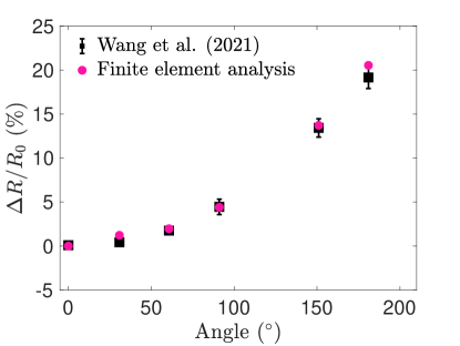
b) c)

Figure 4: Finite element analysis of a resistive strain sensor mounted on a robotic finger-like actuator from Wang et al. (2021). a) Non-dimensional geometry of the device. On face 4 the four outer nodes are pinned, and the two midplane nodes are given matching applied displacement, to drive a three point bending deformation. b) Deformation comparison between the simulation results and the experimental images. The pink color in the top row denotes the deformed finite element mesh. The closeup views below show the true strain component (${\bf\epsilon}^{t}_{11}$) from our finite element analysis. c) Comparison of the relative resistance obtained from finite element analysis and experiments. Here, $R_{0}$ denotes the initial resistance, i.e., the resistance at 0^∘.

Comparison between the simulation predictions and the experimental data is presented in Figures 4b and 4c. In Figure 4b we show the deformed simulated sensor on top of the experimental images; the insets show closeup views of the sensor with true strain component ${\bf\epsilon}^{t}_{11}$ obtained from simulations. Mechanical deformation is in good qualitative agreement with the experimentally observed sensor geometry. As in the experiments, we observe a deformation-driven increase in resistance with the increase in bending angle, shown in Figure 4c. Due to elongation, i.e. the increase in contour path between faces 1 and 2, the electric field and the concentration gradients decrease. Therefore, the ionic flux is reduced for a given applied voltage, and consequently, we observe greater resistance as the sensor undergoes bending. The resistance obtained from the finite element analysis closely matches the experimental measurements, thus proving the developed model is able to simulate operation of resistive ionotronic sensors.

3.3.2 Ionic junctions

Next, we demonstrate the modeling and simulation capabilities on energy harvesting devices based on ionic junctions. These ionic junctions involve an interface between two polymer membranes with opposite fixed charge; i.e. one layer is a polyanion and the other layer is a polycation. Each membrane initially contains sufficient mobile counter ions to result in an overall neutral material. A neutral fixed charge region exists between the two layers either through explicit incorporation of a neutral separator or from interdiffusion of the polymer chains from each membrane. When joined, ions at the interface diffuse across the neutral layer and into the other polymer due to the large initial chemical potential gradient at the junction. This initial migration of mobile ions leaves the backbone charge of the material near the neutral layer unbalanced. Consequently, an electric field is established between the polyanion and polycation. Electrodes are typically placed on each side of the junction, measuring the difference in voltage as an open circuit electric potential. Once the entropically driven migration is balanced by the internal electric field, the ionic junction is at equilibrium, characterized by the equilibrium electric potential $\varphi_{eq}$.

Before moving on to describing the device operation, to help discuss the performance of these devices, we make certain analogies to electric circuits. Assuming blocking electrodes, these systems can be considered as ideal capacitors; the relation of the bulk capacitance to the electrode-to-electrode distance $d$ and cross-sectional area $A$ is given by

$$\mathcal{C}=\varepsilon\,\frac{A}{d}\,$$ (24)

Therefore, both decrease in electrode-to-electrode distance and increase in cross-sectional area correspond to an increase in device capacitance. In addition, capacitance can be also represented as the ratio of the charge density at the capacitor plates to the electric potential between them.

$$\mathcal{C}=\rho/\varphi,$$ (25)

In this section we will discuss operation of two devices (Figure 5) relying on ionic junctions to transduce mechanical deformation and stress into electric potential (measured as open circuit potential): (i) a device developed by Hou et al. (2017) (the version without carbon nanotube enhancement), and (ii) a device published by. Kim et al. (2020). The operation of both devices involves a change in the electrode-to-electrode distance (alternating decreasing and increasing) and the cross-sectional area (alternating increasing and decreasing). The first operates via through-plane compression while the latter operates via in-plane extension. Two other key differences are the material properties and the neutral layer composition. The first system uses leathery polymers (developed as fuel cell membranes) with a porous polycarbonate separator and the second system uses ionogels without any separator. Both systems have relatively large counter ions. Because of the material property differences and choices of the authors, the Hou et al. system is characterized with on/off steps in stress every $70\,$s corresponding to $\sim 0.03\%$ strain whereas the Kim et al. system is characterized with a pre-stretch of 1.2 and a superposed sinusoid of amplitude 0.15 and frequency of 1 Hz. In addition to predicting performance of these two devices with our best approximation of each system, we will use these cases to study sensitivity to our assumptions and understand the drivers of good device performance. We are especially interested in the seemingly simple question - what drives the open circuit voltage to increase or decrease under mechanical deformation?

a)	b)
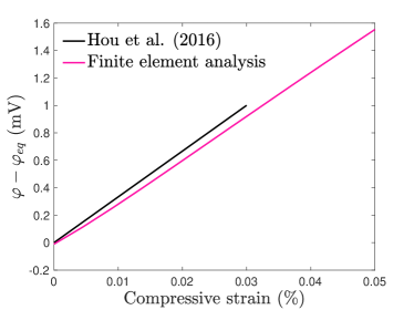
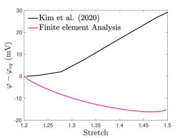
c)	d)

Figure 5: Ionic device summary. Device geometry for a) Nafion/DF25 ionic junction Hou et al. (2017), and b) ES/AT ionic junction Kim et al. (2020). The blue and orange colors denote regions with negatively and positively charged polymer backbone, respectively. The gray color denotes regions with neutral backbone charge, and circles denote the mobile ions at $t=0$. The meshed region is indicated with thick black lines. Note: geometry is not drawn to proportion. Electric potential across the junction (i.e., between the top and bottom face) under mechanical loading and open circuit condition: c) in Nafion/DF25 for compression in the 1-direction, and d) in ES/AT for elongation in the 2-direction. Experimental data is plotted alongside simulation results for comparison.

3.4 Simulation results for Hou et al. (2017) junction

The device consists of two oppositely charged membranes, Nafion and DF25 (poly(2,6-dimethyl- 1,4-phenylene oxide (PPO)) with quaternary ammonium bromide side chains, each $12\,\mu$m thick, separated by a $6\,\mu$m thick layer of porous polycarbonate. In our simulation, we consider a region involving a $6\,\mu$m separator, and $2\,\mu$m regions of the ion exchange membranes on each side of the separator, thus the total length of the meshed region is $L=10\,\mu$m (further discussion on the size of the region under consideration is provided in B). The meshed region is denoted with thick black lines in Figure 5a, and consists of 300 3D elements, with a single element in 1-direction (in B we provide justification for this choice). Each element is $0.33\cdot 10^{-2}\,L$ long, $L$ wide and thick.

As with the previous device, we will describe this system using dimensional parameters. The open circuit potential is computed as the difference between the electric potential at nodes initially at $x_{1}=-5\,\mu$m and $x_{1}=5\,\mu$m. We consider low mobile ion concentration on the order of mM, as suggested in Zhou et al. (2017).The diffusivity $D=10^{-9}$m²/s is typical for such ion exchange membranes. The charge numbers for positive and negative ions are $z^{(+)}=1\,$ and $z^{(-)}=-1\,$, respectively. The dielectric constant $\varepsilon_{R}=20$ (Paddison et al., 1998) corresponds to a Debye length $\lambda_{D}=6\,$nm at $T=293\,$K. We take the volume of both positive and negative ions $\Omega^{(+,-)}=\Omega^{(\text{H}_{2}\text{0})}=1.8\cdot 10^{-5}\,$m³/mol. The shear modulus for all three materials $G=350\,$MPa is based on the uniaxial compression data performed on the entire device. We consider both membranes equally compressible, with a bulk modulus $K=G$, which is equivalent to a Poisson’s ratio of 1/3. We also take the porous separator to have a bulk modulus of $K=G/3$, corresponding to a Poisson’s ratio of 0. The initial conditions are based on the reported material structure, and are given in Table 3. The boundary conditions in effect throughout the simulation are prescribed as follows:

• electric potential boundary condition $\varphi=0$ is prescribed at the interface ($x_{1}=0$); i.e. choosing to ground the device at this location.

• zero flux boundary conditions prescribed on top and bottom surface (initially at $x_{1}=5\,\mu$m and $-5\,\mu$m, respectively) as $\breve{j}^{(+,-)}=0\,$,

• mechanical symmetry boundary conditions prescribed to nodes on face 1 (1-3 plane) and face 2 (1-2 plane), and the displacement of nodes at the interface ($x_{1}=0$) is constrained in 1-direction.

The simulation involves three distinct steps:

1. Allowing the electric potential across the junction to equilibrate, while keeping the above mentioned boundary conditions.

2. Prescribing mechanical displacement in the 1-direction to nodes at the top and bottom surface to compress the device by 5%.

3. Allowing the electric potential to equilibrate again in the compressed configuration.

Parameter	Unit	Nafion	DF25	Separator
$\varphi_{0}$	$\left(\text{V}\right)$	0	0	0
$c^{(+)}_{0}$	$\left(\text{mol/m}^{3}\right)$	1	0	0
$c^{(-)}_{0}$	$\left(\text{mol/m}^{3}\right)$	0	1	0
$c^{(\text{fix})}_{0}$	$\left(\text{mol/m}^{3}\right)$	1	1	0
$z^{(\text{fix})}$		-1	1	0
$G$	$\left(\text{MPa}\right)$	350	350	350
$K/G$		1	1	1/3

Table 3: Initial conditions and material parameters for simulating Nafion/DF25 ionic junction by Hou et al. (2017).

Simulation results in Figure 6a show that the initial, entropically driven, diffusion of ionic species stops after $t\approx 0.05\,$ms. The established electric field prevents further ion migration, and the electric potential between the top and bottom face reaches equilibrium at $\varphi_{eq}\approx 195\,$mV. We also observe that the mechanical deformation during the second step induces an increase in electric potential across the junction. In Figure 6b, we show the net charge density $\rho$ and ion concentration when undeformed and when compressed by 5%. The depletion of mobile ions close to the polyelectrolyte/separator interface is caused by the migration of ions into the separator during underformed equilibration. Consequently, the fixed charges in the depletion region are no longer balanced by the counterions, increasing the net charge density at the interface, and thus generating an electric potential across the junction. When compressed, gradients of the electric potential and of the chemical potential are equally increased across the junction through affine deformation of the fixed and mobile charges. Since the two gradients, which are the driving force for the diffusion based on the flux relation in (21), have equal and opposite effect on the movement of mobile ions, no further ion migration takes place. As expected, once compressed, the overall increase in ion concentration yields a higher electric potential across the junction; and a similar observation was also made by Zhou et al. (2017). While we observe the same voltage trend as in the experiment, the increase in voltage at $0.03\%$ compressive strain is $\approx 10$% less than the experimentally observed one (see Figure 5c).

The particular device design also imposes a multiphysics problem with significantly different time scales between the electrochemical phenomena ($\sim\,$ms) and the applied mechanical load ($\sim 10\,$s). As previously mentioned, we non-dimensionalize the simulation time domain based on the electrochemical parameters: diffusivity coefficient, the length of the system under consideration, and the Debye length. For this system, the time normalization factor $\approx 2\cdot 10^{4}$s^-1 maps a non-dimensional time increment of $\tau=1$ to $t=0.05\,$ms. Consequently, our simulation environment is more conveniently set to capture the electrochemical processes, while the much slower mechanical loading rate requires an extensively long simulation time. Therefore, we ran a set of simulations to investigate the effects of mechanical loading rate on the electrochemical performance. We conducted a set of simulations at four different mechanical compression rates d$\lambda$/d$\tau=1\cdot 10^{-1}\,$, $5\cdot 10^{-2}$, $1\cdot 10^{-2}$, and $5\cdot 10^{-3}$, to 5% strain, while keeping the remaining parameters and boundary conditions the same as in the initial simulation.

In Figure 6c, we show the device response to different mechanical compression rates as the difference between electric potential in current configuration and in undeformed configuration at equilibrium. The loading rate in our initial simulation is d$\lambda$/d$\tau=1\cdot 10^{-2}$. While the steady-state open circuit voltage has negligible dependence on the loading rate, the approach to that value does depend on the loading rate. The faster the loading rate, the larger the overshoot, and the larger the undershoot (though this is much less in magnitude than the overshoot). For all rates, there is a gradual increase to the final value. Similar peaks, followed by a new equilibrium state, have also been observed through experimental characterization of this system by Hou et al. (2017).

a)	b)

c)

Figure 6: Simulation results for Nafion/DF25. a) Electric potential across the junction under open circuit condition during equilibration step and while compressing. b) Concentration of net charge and mobile ions across the junction when undeformed and at equilibrium and when compressed by 5% and at the new equilibrium. c) Influence of mechanical compression rate on the electrochemical behavior. Simulations are performed at d$\lambda$/d$\tau=1\cdot 10^{-1}\,$, $5\cdot 10^{-2}$, $1\cdot 10^{-2}$, and $5\cdot 10^{-3}\,$. The pink line represents the same deformation rate as in a). Arrow indicates increase in the compression rate.

3.5 Simulation results for Kim et al. (2020) junction

The reported device consists of two $250\,\mu$m thick sheets of ES (poly(1-ethyl-3-methyl imidazolium (3-sulfopropyl) acrylate)) with EMIM⁺ ( 1-ethyl-3-methylimidazolium) mobile ions and AT (poly(1-[2-acryloyloxyethyl]-3-butylimidazolium bis(trifluoromethane) sulfonimide)) with TFSI^- (bis(trifluoromethane) sulfonimides) mobile ions. To simulate the operation of this ionotronic device, we mesh $L=1\,\mu$m ($0.5\,\mu$m on each side of the interface); further discussion on the effects of $L$ under consideration can be found in B. The finite element mesh consists of 2000 3D elements in 1-direction, each $5\cdot 10^{-4}\,L$ long, and $10\,L$ wide and thick, with a single element in the cross-section.

As in the experiments, the ES region has negative fixed charge combined with mobile positive ions, while the AT region contains positive fixed charge and negative mobile ions. The initial conditions are based on the reported preparation procedure and experimental setup, and are provided in Table 4. As suggested in Kim et al. (2020), we assume low degree of ionization, and take concentration of ions on the order of  mM, and a diffusion coefficient $D=10^{-14}$m²/s based on the reported conductivity. The dielectric constant $\varepsilon_{R}=15$ is common for ionic liquids (cf. e.g., Weingaertner, 2014), and yields a Debye length of $\lambda_{D}\approx 6\,$nm at $T=293\,$K. The molar volume of these ionic liquids is $\Omega^{(+)}=1.4\cdot 10^{-4}$m³/mol and $\Omega^{(-)}=1.9\cdot 10^{-4}$m³/mol. The shear modulus for both materials $G=38\,$kPa is based on the uniaxial tensile testing performed on ES/AT junction. In our initial simulation, we assume that the materials are compressible, more specifically $K=G$. We also set the thickness of the neutral interface between the two ionogels to be $t_{n}=10\,$nm, and assume it has the same mechanical properties as the pure polyanion and polycation regions. The boundary conditions set throughout the simulation are as follows:

• electric potential boundary condition $\varphi=0$ is prescribed at the interface ($x_{1}=0\,$); i.e. choosing to ground voltage at this position,

• zero flux boundary conditions prescribed on the top and bottom surfaces (initially at $x_{1}=0.5\,\mu$m and $x_{1}=-0.5\,\mu$m), as $\breve{j}^{(+,-)}=0\,$,

• symmetry boundary conditions are prescribed at nodes on the face 1 (1-3 plane) and face 2 (1-2 plane), and the displacements of nodes at the interface ($x_{1}=0$) are constrained in the 1-direction.

Parameter	Unit	ES	AT	Neutral layer
$\varphi_{0}$	$\left(\text{V}\right)$	0	0	0
$c^{(+)}_{0}$	$\left(\text{mol/m}^{3}\right)$	1	0	0.5
$c^{(-)}_{0}$	$\left(\text{mol/m}^{3}\right)$	0	1	0.5
$c^{(\text{fix})}$	$\left(\text{mol/m}^{3}\right)$	1	1	0
$z^{(\text{fix})}$		-1	1	0
$G$	$\left(\text{MPa}\right)$	38	38	38
$K/G$		1	1	1

Table 4: Initial conditions and material parameters for simulating ES/AT junction by Kim et al. (2020).

The simulation involves three distinct steps:

1. Allowing the electric potential across the junction to equilibrate, while keeping the above mentioned boundary conditions.

2. Prescribing the mechanical displacement along the 2-direction to nodes on face 3 (located opposite of the face 1) to reach the stretch $\lambda=1.2$, and allowing the electric potential to equilibrate again.

3. Prescribing the mechanical displacement to nodes at face 3 to match the experimentally applied stretch $\lambda_{\,\text{sin}}$. The displacement is applied along the 2-direction in the form of a sinusoidal wave.

Simulation results in Figure 7a show that the equilibrium electric potential $\varphi_{eq}=80\,$mV in the undeformed configuration is established after approximately $10\,$s. We observe a decrease in electric potential while the device is stretching to $\lambda=1.2$ in the 2-direction; and this trend extends onto the next step, when the device is subjected to a cycling stretch $\lambda_{\text{sin}}$. On the other hand, reported device performance follows the opposite trend, i.e., an increase in electric potential with elongation in the 2-direction (see Figure 5d).

The decrease in interface thickness brings the polyanion and polycation networks closer, corresponding to an increase in the electric field (i.e., electric potential is acting over shorter distance). However, the net charge concentration $\rho$ slightly decreases when elongated to $\lambda=1.5$, as shown in Figure 7b; this effect can be attributed to compressibility as suggested by the drop in ion concentration (this is opposite the device Hou et al. (2017) for which compression was applied). Following Gauss’s law (8), the electric potential needs to decrease to satisfy both the decrease in thickness and the decrease in net charge density. While the computational predictions provide a reasonable and expected dependence between the elongation and electric potential, the experimental data clearly exhibits the opposite trend, as observed in Figure 5d. Moreover, in Figure 7c we show the comparison between the simulation results and experimental data while the device is undergoing cyclic loading $\lambda_{\text{sin}}\,$, where we also observe the same/non-matching trends in electrochemical response to an applied mechanical stretch.

In addition to the numerical approach, an analogy between this ionic junction and a capacitor in an electrical circuit provides more insights on the expected device performance. More specifically, elongation in the 2-direction, corresponds to an increase in the cross-sectional area while the electrode-to-electrode distance, i.e., the distance between the top and bottom face, is decreasing. Both geometrical effects yield an increase in capacitance based on equation (24); and the increase in capacitance is also documented by Kim et al. (2020) in their experimental investigation. Therefore, a decrease in the electric potential across the junction is expected based on equation (25) when $\rho$ is constant or decreasing. Nonetheless, the experimental data shows the opposite trend, i.e., the electric potential is increasing with elongation.

a)	b)

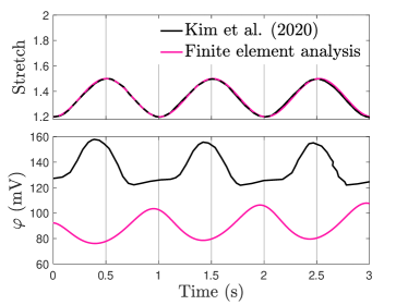
c)

Figure 7: Finite element analysis of energy harvesting device developed by Kim et al. (2020). a) Electric potential across the junction under open circuit condition during equilibration, mechanical loading to $\lambda=1.2$ and second equilibration, and while applying a sinusoidal stretch $\lambda_{\text{sin}}$. b) Concentration of net charge and mobile ions across the junction when undeformed and at equilibrium, and when stretched to 1.5 in the third step. c) Comparison with the experimental data while applying $\lambda_{\text{sin}}$. Grid lines are added to guide the eye.

One possible source for the experimentally observed increase in the electric potential with increasing stretch is a changing neutral layer thickness. As the interpenetrated neutral region is stretched, the tension could tear the polycation and polyanion polymers back apart, decreasing the size of the neutral layer. In order to determine the effect this thickness change might have on the junction potential, we perform an additional set of five simulations with neutral layer thicknesses of $10\,$nm, $20\,$nm, $30\,$nm, $40\,$nm, and $50\,$nm. We are interested mainly in the equilibrium junction potential, and so simulate only the equilibration step.

In Figure 8a we observe an increase in the equilibrium voltage with a decrease in thickness of neutral region between the two oppositely charged polymer networks. This trend holds for all five simulations, and in Figure 8b, we show the net charge and ion concentration profiles across the junction when the neutral layer thickness is $t_{n}=10$ and $50\,$nm. When the neutral region is large compared to the Debye length, the system can be conceptualized as two separate junctions in series. One junction is formed between the polyanion and the neutral region, and the other junction is formed between the neutral region and polycation. These two junctions are the source of the two discontinuities in the slope $\rho$ in Figure 8. Across each junction, the concentration of the dominant mobile species drops by half from the polyion side to the neutral side. For smaller neutral regions, these two junctions begin to overlap, looking more like one junction across which the concentration of each mobile species drops to nearly zero. Because the PNP equations are nonlinear in concentration, the two junction profiles do not superpose. Instead overlapping the junctions with a small neutral layer results in slightly more than double the voltage drop of the individual polyion–neutral junctions. Thus, as the neutral region shrinks, the equilibrium junction voltage increases. Therefore, our computational study shows that a decrease in neutral layer thickness could be responsible for the experimentally measured change in the electric potential.

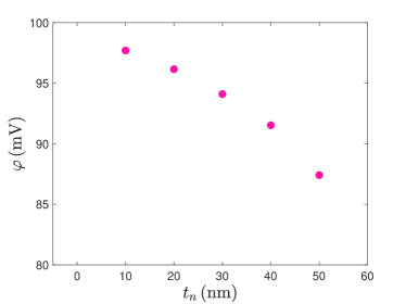
a)	b)

Figure 8: Effect of neutral layer thickness on the equilibrium potential for the energy harvesting device developed by Kim et al. (2020). a) Equilibrium electric potential across the junction obtained at five different neutral layer thickness values $t_{n}=10\,,$ 20, 30, 40, and $50\,$nm. b) Net charge density and concentration of mobile species at the end of equilibration step for $t_{n}=10\,$ and $50\,$nm.

Next, we probe the effects of material compressibility on the overall electrochemical behavior of the junction. To investigate the influence of this feature, we perform a set of simulations at different bulk-to-shear modulus ratios $K/G$. More specifically, we simulate the response of an incompressible material ($K/G=100$), and then compare the simulation results with the initial case ($K/G=1$). The remaining material parameters, as well as boundary conditions, are kept the same as in the initial simulation, and we repeat all three simulation steps.

Figure 9a shows the device performance at two different shear-to-bulk-modulus ratios during the equilibration step, while loading to $\lambda=1.2$, and under a cyclic load $\lambda_{\text{sin}}$. Compressibility significantly increases the coupling between the applied mechanical deformation and electric potential, observed as a steeper decrease in potential while stretching, and, similarly, a larger amplitude under cyclic load. As expected, the increase in volume due to a tensile load causes the charge density to decrease, thus yielding a lower electric potential across the junction. This is further corroborated by the net charge and ion concentration profiles when stretched to $\lambda=1.5$, shown in Figure 9b. The net charge and ion concentration are decreasing with elongation when considering the material as a compressible solid, and remain almost constant when nearly incompressible. The decrease in concentration, coupled with a decrease in distance between the polyanion and polycation layer, yields a lower electric potential across the junction.

One aspect of the device performance we have not investigated in this work is the effect of the dispersed carbon nanotube (CNT) electrodes on the overall electro-chemo-mechanical response. Films of randomly dispersed CNTs are embedded on both sides of ES/AT junctions, acting as high surface area electrodes. Because of the rigidity of individual CNTs relative to the CNT network, the CNT electrode area is independent of ionoelastomer deformation. A major implication of such electrode behavior is that the surface area at the CNT/ES and CNT/AT interface remains constant, while ES/AT interface area is increasing. Consequently, the experimentally observed increase in junction capacitance with in-plane extension is mainly attributed to increasing ES/AT interface area, and also to decreasing distance between the electrodes. In current literature, the effect of high surface area electrodes on the electrochemical response of ionic polymers is captured either by increasing diffusion coefficient and dielectric permittivity values close to the electrodes (cf., e.g., Wallmersperger et al., 2008), or by modeling small particles within the polymer matrix (cf., e.g., Akle et al., 2011). However, current models do not capture the coupled influence of mechanical deformation and the electrochemical response of CNT network and polymer matrix.

Lastly, we note that unlike the previous Nafion/DF25 based device, the difference in timescales between the electrochemical phenomena and the applied mechanical deformation is significantly smaller for ES/AT ionic junction. This is mainly due to three orders of magnitude lower diffusion coefficient; and is also caused by a significantly faster mechanical excitation of $1\,$Hz. Here, the time normalization factor is $\approx 170\,$s^-1, mapping each non-dimensional time increment $\tau=1$ to $t=6\,$ms.

a)	b)

Figure 9: Sensitivity of the device performance to compressibility for the energy harvesting device developed by Kim et al. (2020). a) Electric potential across the junction under open circuit condition during equilibration step, mechanical loading to $\lambda=1.2$, and while applying a sinusoidal stretch $\lambda_{\text{sin}}$, at two different bulk-to-shear modulus ratios: 1 and 100. b) Net charge density and concentration of mobile species when stretched to $\lambda=1.5$ for both bulk-to-shear modulus ratios.

4 Conclusion

We have developed a continuum-level multiphysics framework and a constitutive model for the electro-chemo-mechanically coupled behavior of soft ionic conductors. Our modeling approach takes into account the influence of electric fields, the diffusion of multiple ionic species, the influence of fixed charge groups, and mechanical deformation. Both the framework and the model are numerically implemented for use in finite element analysis. We developed two custom finite element codes: (i) a 1D electrochemical version in Matlab and (ii) a coupled electro-chemo-mechanical version, implemented as a user element (UEL) Abaqus subroutine for use in general 3D boundary value problems. We verified and validated our numerical approach by comparing the finite element analysis with the analytical results and EIS data, respectively. Next, we showcased the usefulness of our tool to accurately capture the change in resistance due to applied mechanical deformation in a hydrogel-based sensor. Finally, we utilized the developed computational tool to analyze the response of two devices involving ionic junctions between polyanionic and polycationic polymer networks. Simulation results helped build understanding of the influence of deformation and mechanical properties on the behavior of these electrochemical systems. More specifically, we investigated the influence of mechanical loading rate, separation between the charged networks, and compressibility, on the performance of ionotronic devices involving junctions between oppositely charged networks. Towards the future, we aim to extend our model to account for the effects of electrode nanostructure, such as CNT networks, on the overall response of the device, as well as the diffusion and interpenetration of polymer chains at the ionic interface between oppositely charged networks. As we continue our experimental characterization of ionotronic materials, we are looking to improve our model to accurately capture the influence of multiple mobile species. Finally, the developed computational tool can be used for design of novel ionotronic devices.

Acknowledgments

The authors acknowledge the support through the Defense Advanced Research Project Agency Young Faculty Award (DARPA YFA; HR00112010004). The authors would also like to acknowledge Prof. Hyeong Jun Kim at Sogang University for sharing his perspectives on the behavior of ionoelastomer junctions.

Appendix A Numerical implementation

We make use of the finite element method to solve the governing relations, represented by a set of coupled partial differential equations in (8), (10) and (11), following the approach laid out in Chester et al. (2015). To find the solutions for this multiphysics probelem, we utilize the Newton-Raphson iterative method and specify a set of element-level residuals and tangents. The developed numerical method is implemented in the form of custom finite element codes in: (i) Matlab and Python as a 1D electrochemical code (i.e. in the absence of mechanical deformation), and (ii) in Abaqus/Standard as a user element (UEL) subroutine.

To numerically implement the developed framework, first, we define the strong forms, consisting of balance laws and the corresponding boundary conditions. The strong form for Gauss’s law is given by:

$$\left.\begin{aligned} \hbox{{Div}}\mskip 2.0mu{\bf d}&=eN_{a}\rho\quad&\text{in}\quad\mathcal{B},\\ {\bf d}\cdot{\bf n}&=\breve{q}\quad&\text{on}\quad\mathcal{S}_{q},\\ \varphi&=\breve{\varphi}\quad&\text{on}\quad\mathcal{S}_{\varphi}.\end{aligned}\right\}$$ (26)

where ${\bf n}$ is the outward unit normal, and $\breve{q}$ and $\breve{\varphi}$ represent the prescribed surface charge and electric potential, respectively, on two complementary surfaces $\mathcal{S}_{\Omega}$ and $\mathcal{S}_{\varphi}$.

The balance of mass, along with boundary conditions, takes the form:

$$\left.\begin{aligned} \dot{c}^{(i)}&=-\hbox{{Div}}\mskip 2.0mu{\bf j}^{(i)}\quad&\text{in}\quad\mathcal{B},\\ {\bf j}^{(i)}\cdot{\bf n}&=\breve{j}^{(i)}\quad&\text{on}\quad\mathcal{S}_{\bf j},\\ \mu^{(i)}&=\breve{\mu}^{(i)}\quad&\text{on}\quad\mathcal{S}_{\mu}.\end{aligned}\right\}$$ (27)

with $\breve{j}$ and $\breve{\mu}$ denoting the prescribed ion flux and chemical potential, respectively, on two complementary surfaces $\mathcal{S}_{\bf j}$ and $\mathcal{S}_{\mu}$.

Finally, the strong form for balance of forces is:

$$\left.\begin{aligned} \hbox{{Div}}\mskip 2.0mu{\bf T}+{\bf b}&=\bf 0\quad&\text{in}\quad\mathcal{B},\\ {\bf T}{\bf n}&=\breve{{\bf t}}\quad&\text{on}\quad\mathcal{S}_{\bf t},\\ {\bf u}&=\breve{{\bf u}}\quad&\text{on}\quad\mathcal{S}_{\bf u}.\end{aligned}\right\}$$ (28)

where ${\bf u}$ is the displacement, and $\breve{{\bf t}}$ and $\breve{{\bf u}}$ are the prescribed surface traction and displacement, respectively, on two complementary surfaces $\mathcal{S}_{\bf t}$ and $\mathcal{S}_{\bf u}$.

The body $\mathcal{B}$ is then approximated with finite elements, such that $\mathcal{B}=\cup\mathcal{B}^{e}$. Further, we consider the electric potential $\varphi$, the chemical potential $\mu^{(i)}$ and the displacement ${\bf u}$ as the nodal degrees of freedom (DOFs). The nodal DOFs are evaluated within each element using the shape functions $N^{A}$

$$\varphi=\sum\varphi^{A}N^{A}\,,\quad\mu^{(i)}=\sum\left(\mu^{(i)}\right)^{A}N^{A}\quad\text{and}\quad{\bf u}=\sum{\bf u}^{A}N^{A}\,,$$ (29)

where $A$ denotes the element nodes.

Based on the strong forms in (26), (27) and (28), and using the divergence theorem, we develop weak forms and obtain the element-level residuals for each of the nodal DOF’s:

$$\begin{split}\left(R_{\varphi}\right)^{A}&=\int_{\mathcal{B}^{e}}N^{A}\rho\,\text{dv}+\int_{\mathcal{B}^{e}}\nabla N^{A}\,{\bf d}\,\text{dv}-\int_{{\mathcal{S}_{q^{e}}}}N^{A}\breve{q}\,\text{da}\,,\\ \left(R_{\mu(i)}\right)^{A}&=\int_{\mathcal{B}^{e}}N^{A}\dot{c}_{\textrm{\tiny R}}^{(i)}\,\text{dv}+\int_{\mathcal{B}^{e}}\nabla N^{A}J{\bf j}^{(i)}\,\text{dv}-\int_{{\mathcal{S}_{{\bf j}^{e}}}}N^{A}\breve{j_{\textrm{\tiny R}}}^{(i)}\,\text{da}\,,\\ \left({\bf R}_{\bf u}\right)^{A}&=-\int_{\mathcal{B}^{e}}\nabla N^{A}{\bf T}\,\text{dv}+\int_{{\mathcal{S}_{{\bf t}^{e}}}}N^{A}\,\breve{t}\,\text{da}\,.\end{split}$$ (30)

To provide a convenient set of numbers to the Newton-Raphson solver, we non-dimensionalize the electrochemical quantities, and introduce the non-dimensional electric potential, chemical potential, and charge concentration

$$\Phi=\varphi\frac{eN_{a}}{RT}\,,\quad\textrm{M}=\frac{\mu}{RT}\,\textrm{, and}\quad C=\frac{c}{c^{E}}\,,$$ (31)

respectively. Considering (30) and (31), we obtain the non-dimensionalized electrochemical residuals as

$$\begin{split}\left(R_{\Phi}\right)^{A}&=\int_{\mathcal{B}^{e}}N^{A}P\,\text{dv}-\int_{\mathcal{B}^{e}}\frac{\partial N^{A}}{\partial X}\lambda_{D}^{2}L^{-2}\frac{\partial\Phi}{\partial X}\,\text{dv}-\int_{{\mathcal{S}_{q^{e}}}}N^{A}\breve{Q}\,\text{da}\,,\\ \left(R_{M(i)}\right)^{A}&=\int_{\mathcal{B}^{e}}N^{A}\frac{\partial C_{\textrm{\tiny R}}^{(i)}}{\partial\tau}\,\text{dv}-\int_{\mathcal{B}^{e}}\frac{\partial N^{A}}{\partial X}JC^{(i)}\lambda_{D}L^{-1}\left(\frac{\partial M^{(i)}}{\partial X}+z^{(i)}\frac{\partial\Phi}{\partial X}\right)\,\text{dv}\\ &\quad-\int_{{\mathcal{S}_{{\bf j}^{e}}}}N^{A}\breve{J}^{(i)}\,\text{da}\,,\end{split}$$ (32)

where $P=\sum_{i}\left(z^{(i)}C^{(i)}\right)+z^{\text{(fix)}}C^{\text{(fix)}}$ is the non-dimensional net charge density.

In addition to non-dimensionalized element-level residuals, we provide a set of non-dimensionalized element-level tangents required to orient the Newton-Raphson solver. The tangents for non-dimensionalized electric potential are obtained as

$$\begin{split}\left(K_{\Phi\Phi}\right)^{AB}&=-\mbox{$\dfrac{\partial\left(R_{\Phi}\right)^{A}}{\partial{\Phi^{B}}}$}=\int_{\mathcal{B}^{e}}\frac{\partial N^{A}}{\partial X}\lambda_{D}^{2}L^{-2}\frac{\partial N^{B}}{\partial X}\,\text{dv}\,,\\ \end{split}$$ (33)

and

$$\begin{split}\left(K_{\Phi M(i)}\right)^{AB}&=-\mbox{$\dfrac{\partial\left(R_{\Phi}\right)^{A}}{\partial{\left(M^{(i)}\right)^{B}}}$}=-\int_{\mathcal{B}^{e}}N^{A}N^{B}z^{(i)}\frac{\partial C_{\textrm{\tiny R}}^{(i)}}{\partial M^{(i)}}\,\text{dv}.\\ \end{split}$$ (34)

Similarly, the non-dimensionalized chemical potential tangents are given by

$$\begin{split}\left(K_{M(i)M(i)}\right)^{AB}&=-\mbox{$\dfrac{\partial\left(R_{M(i)}\right)^{A}}{\partial{\left(M^{(i)}\right)^{B}}}$}\\ &=-\int_{\mathcal{B}^{e}}N^{A}N^{B}\mbox{$\dfrac{\partial\left(\partial C_{\textrm{\tiny R}}^{(i)}/\partial\tau\right)}{\partial{M^{(i)}}}$}\,\text{dv}\\ &\quad+\int_{\mathcal{B}^{e}}J\lambda_{D}L^{-1}\mbox{$\dfrac{\partial N^{A}}{\partial{X}}$}\left(N^{B}\mbox{$\dfrac{\partial C^{(i)}}{\partial{M^{(i)}}}$}\left(\mbox{$\dfrac{\partial M^{(i)}}{\partial{X}}$}+z^{(i)}\mbox{$\dfrac{\partial\Phi}{\partial{X}}$}\right)+C^{(i)}\mbox{$\dfrac{\partial N^{B}}{\partial{X}}$}\right)\,\text{dv}\,,\end{split}$$ (35)

and

$$\begin{split}\left(K_{M(i)\Phi}\right)^{AB}&=-\mbox{$\dfrac{\partial\left(R_{M(i)}\right)^{A}}{\partial{\Phi^{B}}}$}\\ &=\int_{\mathcal{B}^{e}}J\lambda_{D}L^{-1}\mbox{$\dfrac{\partial N^{A}}{\partial{X}}$}z^{(i)}C^{(i)}\mbox{$\dfrac{\partial N^{B}}{\partial{X}}$}\,\text{dv}\,.\\ \end{split}$$ (36)

Appendix B Influence of geometrical features and finite element mesh on simulation results

In this section we discuss the sensitivity of simulation results to geometrical features and finite element mesh. Throughout this section we consider a region consisting of two oppositely charged polymeric backbones, with geometrical parameters labeled as the length $L$, width $W$, and neutral layer thickness $t_{n}$, as shown in Figure 10. The geometry is meshed with 1000 3D elements, each $1\,$nm long, and $1\,\mu$m thick and wide, unless otherwise specified. We take molar volume of both species $\Omega^{(i)}=10^{-4}\,$mol/m³, and the Debye length $\lambda_{D}=10\,$nm. The remaining material parameters and initial conditions are provided in Table 5. Simulations consist of equilibration step over a non-dimensionalized time interval $\tau=8\,$, and we focus our attention on the electric potential between the top ($x_{1}=L/2$) and the bottom ($x_{1}=-L/2$) face. The boundary conditions are as follows:

• electric potential boundary condition $\varphi=0$ is prescribed at the interface ($x_{1}=0\,$); i.e. choosing to ground voltage at this position,

• zero flux boundary conditions prescribed on the top and bottom surfaces (at $x_{1}=-L/2$ and $x_{1}=L/2$), as $\breve{j}^{(+,-)}=0\,$,

• symmetry boundary conditions are prescribed to nodes at face 1 (1-3 plane) and face 2 (1-2 plane), and the displacements of nodes at the interface ($x_{1}=0$) are constrained in the 1-direction.

Figure 10: Geometry for investigating the effects of geometrical features and finite element mesh.

Parameter	Unit	Polyanion	Polycation	Neutral layer
$\varphi_{0}$	$\left(\text{V}\right)$	0	0	0
$c^{(+)}_{0}$	$\left(\text{mol/m}^{3}\right)$	1	0	0
$c^{(-)}_{0}$	$\left(\text{mol/m}^{3}\right)$	0	1	0
$c^{(\text{fix})}_{0}$	$\left(\text{mol/m}^{3}\right)$	1	1	0
$z^{(\text{fix})}$		-1	1	0
$G$	$\left(\text{MPa}\right)$	100	100	100
$K/G$		1	1	1

Table 5: Initial conditions and material parameters for investigation of parameter sensitivity.

We first probe the influence of geometrical features: (1) length-to-Debye length ratio $L/\lambda_{D}\,$, and (2) the length-to-width ratio $L/W\,$. Then we compare the simulation results when considering a single element in the cross section against the multiple elements in (3).

1. Sensitivity to $L/\lambda_{D}$
   To investigate the sensitivity to $L/\lambda_{D}$, we conduct a set of simulations at a fixed $\lambda_{D}=10\,$nm, and vary the overall length of the geometry $L=100\,$nm, $200\,$nm, $500\,$nm, $1\,\mu$m, and $2\,\mu$m. In Figure 11a we show the equilibration step results. Here, the electric potential is normalized with $\varphi_{max}=\varphi\left(L/\lambda_{D}=200,\tau=8\right)$, and we observe an increase in electric potential with an increase in $L/\lambda_{D}$. However, once $L/\lambda_{D}>80$, there is no noticeable increase in the electric potential (less than 5% difference), as shown in Figure 11b. Therefore, we take $L/\lambda_{D}=100$ as a region sufficiently long to ensure accuracy of our finite element analysis; and the simulation results for this particular ratio are denoted with pink color in 11.

   a)	b)

   Figure 11: Electric potential across the junction normalized with $\varphi_{max}\left(L/\lambda_{D}=200,\tau=8\right)$ for $L/\lambda_{D}=10$ to $200\,$. Pink line denotes the results obtained at $L/\lambda_{D}=100$, and the green circle represents the maximum electric potential used for normalization. b) Electric potential across the junction at $\tau=8$ as a function of $L/\lambda_{D}$. Arrow indicates increase in $L/\lambda_{D}$.

2. Sensitivity to $L/W$
   Here, we probe the effects of different $W$ values (i.e., the dimensions in 2-direction and 3-direction, with reference to Figure 10). We keep the length $L=1\,\mu$m constant, and perform three simulations with: $W=10\,$nm, $1\,\mu$m, and $10\,\mu$m, corresponding to $L/W=0.1$, $1$, and $10$, respectively. In Figure 12a we show the electric potential normalized with $\varphi_{max}=\varphi\left(L/W=1,\tau=8\right)$ during equilibration step, and we observe identical response regardless of $L/W$. The same conclusion can be reached when comparing the normalized electric potential at $\tau=8$ in Figure 12b.

   a)	b)

   Figure 12: Electric potential across the junction normalized with $\varphi_{max}\left(L/W=1,\tau=8\right)$ for $L/W=1\,,$ $0.1\,,$ and $10\,$. The green circle represents the maximum electric potential used for normalization. b) Electric potential across the junction normalized with $\varphi_{max}$ at $\tau=8$ as a function of $L/W$. Grid lines are added to guide the eye.

3. Sensitivity to the number of finite elements in cross-section
   To ensure we are accurately capturing the device performance with a single finite element in cross-section, we conduct a set of simulations using 4 and 9 finite elements in the cross-section. The results in 13a show the electric potential normalized with $\varphi_{max}=\varphi\left(1\text{ element},\tau=8\right)$ during equilibration step, and the results for different number of elements in cross-section are indistinguishable. Further, in Figure 13b we show the normalized electric potential after completion of equilibration step ($\tau=8$), and we can conclude that having a single element in cross-section is accurately capturing the behavior of electrochemical systems under consideration.

   a)	b)

   Figure 13: Electric potential across the junction normalized with $\varphi_{max}\left(1\text{ element},\tau=8\right)$ when finite element mesh contains 1, 4, and 9 elements in cross-section. The green circle represents the maximum electric potential used for normalization. b) Electric potential across the junction at $\tau=8$ for different number of finite elements in cross-section. Grid lines are added to guide the eye.

References

- Agmon (1995) N. Agmon. The grotthuss mechanism. Chemical Physics Letters, 244(5-6):456–462, 1995.
- Akle et al. (2011) B. J. Akle, W. Habchi, T. Wallmersperger, E. J. Akle, and D. J. Leo. High surface area electrodes in ionic polymer transducers: numerical and experimental investigations of the electro-chemical behavior. Journal of Applied Physics, 109(7):074509, 2011.
- Aureli et al. (2009) M. Aureli, C. Prince, M. Porfiri, and S. D. Peterson. Energy harvesting from base excitation of ionic polymer metal composites in fluid environments. Smart materials and Structures, 19(1):015003, 2009.
- Banerjee and Curtin (2004) S. Banerjee and D. E. Curtin. Nafion® perfluorinated membranes in fuel cells. Journal of fluorine chemistry, 125(8):1211–1216, 2004.
- Bazant et al. (2004) M. Z. Bazant, K. Thornton, and A. Ajdari. Diffuse-charge dynamics in electrochemical systems. Physical review E, 70(2):021506, 2004.
- Bouklas et al. (2015) N. Bouklas, C. M. Landis, and R. Huang. A nonlinear, transient finite element method for coupled solvent diffusion and large deformation of hydrogels. Journal of the Mechanics and Physics of Solids, 79:21–43, 2015.
- Brumleve and Buck (1978) T. R. Brumleve and R. P. Buck. Numerical solution of the nernst-planck and poisson equation system with applications to membrane electrochemistry and solid state physics. Journal of Electroanalytical Chemistry and Interfacial Electrochemistry, 90(1):1–31, 1978.
- Bucci et al. (2014) G. Bucci, S. P. Nadimpalli, V. A. Sethuraman, A. F. Bower, and P. R. Guduru. Measurement and modeling of the mechanical and electrochemical response of amorphous si thin film electrodes during cyclic lithiation. Journal of the Mechanics and Physics of Solids, 62:276–294, 2014.
- Buck (1969) R. Buck. Diffuse layer charge relaxation at the ideally polarized electrode. Journal of Electroanalytical Chemistry and Interfacial Electrochemistry, 23(2):219–240, 1969.
- Cayre et al. (2007) O. J. Cayre, S. T. Chang, and O. D. Velev. Polyelectrolyte diode: nonlinear current response of a junction between aqueous ionic gels. Journal of the American Chemical Society, 129(35):10801–10806, 2007.
- Chen et al. (2014) B. Chen, J. J. Lu, C. H. Yang, J. H. Yang, J. Zhou, Y. M. Chen, and Z. Suo. Highly stretchable and transparent ionogels as nonvolatile conductors for dielectric elastomer transducers. ACS applied materials & interfaces, 6(10):7840–7845, 2014.
- Chen et al. (2017) J. Chen, W. A. Henderson, H. Pan, B. R. Perdue, R. Cao, J. Z. Hu, C. Wan, K. S. Han, K. T. Mueller, J.-G. Zhang, et al. Improving lithium–sulfur battery performance under lean electrolyte through nanoscale confinement in soft swellable gels. Nano letters, 17(5):3061–3067, 2017.
- Chester and Anand (2010) S. A. Chester and L. Anand. A coupled theory of fluid permeation and large deformations for elastomeric materials. Journal of the Mechanics and Physics of Solids, 58(11):1879–1906, 2010.
- Chester et al. (2015) S. A. Chester, C. V. Di Leo, and L. Anand. A finite element implementation of a coupled diffusion-deformation theory for elastomeric gels. International Journal of Solids and Structures, 52:1–18, 2015.
- Choi et al. (2005) P. Choi, N. H. Jalani, and R. Datta. Thermodynamics and proton transport in nafion: Ii. proton diffusion mechanisms and conductivity. Journal of the electrochemical society, 152(3):E123, 2005.
- Corry et al. (2000) B. Corry, S. Kuyucak, and S.-H. Chung. Tests of continuum theories as models of ion channels. ii. poisson–nernst–planck theory versus brownian dynamics. Biophysical Journal, 78(5):2364–2381, 2000.
- Cukierman (2006) S. Cukierman. Et tu, grotthuss! and other unfinished stories. Biochimica et Biophysica Acta (BBA)-Bioenergetics, 1757(8):876–885, 2006.
- De Gennes et al. (2000) P. De Gennes, K. Okumura, M. Shahinpoor, and K. J. Kim. Mechanoelectric effects in ionic gels. EPL (Europhysics Letters), 50(4):513, 2000.
- Doi et al. (1992) M. Doi, M. Matsumoto, and Y. Hirose. Deformation of ionic polymer gels by electric fields. Macromolecules, 25(20):5504–5511, 1992.
- Drozdov and deClaville Christiansen (2015) A. Drozdov and J. deClaville Christiansen. Modeling the effects of ph and ionic strength on swelling of polyelectrolyte gels. The Journal of chemical physics, 142(11):114904, 2015.
- Eisenberg et al. (2011) B. Eisenberg, Y. Hyon, and C. Liu. A mathematical model for the hard sphere repulsion in ionic solutions. Communications in Mathematical Sciences, 9(2):459–475, 2011.
- Flavell et al. (2014) A. Flavell, M. Machen, B. Eisenberg, J. Kabre, C. Liu, and X. Li. A conservative finite difference scheme for poisson–nernst–planck equations. Journal of Computational Electronics, 13(1):235–249, 2014.
- Gabrielsson et al. (2012) E. O. Gabrielsson, K. Tybrandt, and M. Berggren. Ion diode logics for ph control. Lab on a Chip, 12(14):2507–2513, 2012.
- Ganser et al. (2019) M. Ganser, F. E. Hildebrand, M. Kamlah, and R. M. McMeeking. A finite strain electro-chemo-mechanical theory for ion transport with application to binary solid electrolytes. Journal of the Mechanics and Physics of Solids, 125:681–713, 2019.
- Gauss (1877) C. F. Gauss. Theoria attractionis corporum sphaeroidicorum ellipticorum homogeneorum. In Werke, pages 3–22. Springer, 1877.
- Gillespie et al. (2002) D. Gillespie, W. Nonner, and R. S. Eisenberg. Coupling poisson–nernst–planck and density functional theory to calculate ion flux. Journal of Physics: Condensed Matter, 14(46):12129, 2002.
- Golmon et al. (2009) S. Golmon, K. Maute, and M. L. Dunn. Numerical modeling of electrochemical–mechanical interactions in lithium polymer batteries. Computers & Structures, 87(23-24):1567–1579, 2009.
- Hagiri et al. (2021) M. Hagiri, R. Watanabe, A. Hiruta, and K. Kashima. Modification of copper (ii) ion-exchange properties of freestanding alginate membrane by embedding with zeolite. In MATEC Web of Conferences, volume 333, page 04009. EDP Sciences, 2021.
- Han et al. (2018) D. Han, C. Farino, C. Yang, T. Scott, D. Browe, W. Choi, J. W. Freeman, and H. Lee. Soft robotic manipulation and locomotion with a 3d printed electroactive hydrogel. ACS applied materials & interfaces, 10(21):17512–17518, 2018.
- Hong et al. (2008) W. Hong, X. Zhao, J. Zhou, and Z. Suo. A theory of coupled diffusion and large deformation in polymeric gels. Journal of the Mechanics and Physics of Solids, 56(5):1779–1793, 2008.
- Hou et al. (2017) Y. Hou, Y. Zhou, L. Yang, Q. Li, Y. Zhang, L. Zhu, M. A. Hickner, Q. Zhang, and Q. Wang. Flexible ionic diodes for low-frequency mechanical energy harvesting. Advanced Energy Materials, 7(5):1601983, 2017.
- Jung et al. (2010) J.-H. Jung, S. Vadahanambi, and I.-K. Oh. Electro-active nano-composite actuator based on fullerene-reinforced nafion. Composites science and technology, 70(4):584–592, 2010.
- Kaklamani et al. (2014) G. Kaklamani, D. Cheneler, L. M. Grover, M. J. Adams, and J. Bowen. Mechanical properties of alginate hydrogels manufactured using external gelation. Journal of the mechanical behavior of biomedical materials, 36:135–142, 2014.
- Keller et al. (2011) K. Keller, T. Wallmersperger, B. Kröplin, M. Günther, and G. Gerlach. Modeling of temperature-sensitive polyelectrolyte gels by the use of the coupled chemo-electro-mechanical formulation. Mechanics of Advanced Materials and Structures, 18(7):511–523, 2011.
- Kim et al. (2007) D.-H. Kim, J.-H. Ahn, H.-S. Kim, K. J. Lee, T.-H. Kim, C.-J. Yu, R. G. Nuzzo, and J. A. Rogers. Complementary logic gates and ring oscillators on plastic substrates by use of printed ribbons of single-crystalline silicon. IEEE Electron Device Letters, 29(1):73–76, 2007.
- Kim et al. (2020) H. J. Kim, B. Chen, Z. Suo, and R. C. Hayward. Ionoelastomer junctions between polymer networks of fixed anions and cations. Science, 367(6479):773–776, 2020.
- Kim and Tadokoro (2007) K. J. Kim and S. Tadokoro. Electroactive polymers for robotic applications. Artificial Muscles and Sensors, 23:291, 2007.
- Kornyshev and Vorotyntsev (1981) A. A. Kornyshev and M. A. Vorotyntsev. Conductivity and space charge phenomena in solid electrolytes with one mobile charge carrier species, a review with original material. Electrochimica Acta, 26(3):303–323, 1981.
- Lacour et al. (2016) S. P. Lacour, G. Courtine, and J. Guck. Materials and technologies for soft implantable neuroprostheses. Nature Reviews Materials, 1(10):1–14, 2016.
- Lee et al. (2012) J. Lee, P. Lee, H. Lee, D. Lee, S. S. Lee, and S. H. Ko. Very long ag nanowire synthesis and its application in a highly transparent, conductive and flexible metal electrode touch panel. Nanoscale, 4(20):6408–6414, 2012.
- Leichsenring and Wallmersperger (2017) P. Leichsenring and T. Wallmersperger. Modeling and simulation of the chemically induced swelling behavior of anionic polyelectrolyte gels by applying the theory of porous media. Smart Materials and Structures, 26(3):035007, 2017.
- Li et al. (2001) T. Li, A. Wlaschin, and P. B. Balbuena. Theoretical studies of proton transfer in water and model polymer electrolyte systems. Industrial & engineering chemistry research, 40(22):4789–4800, 2001.
- Li et al. (2017) T. Li, G. Li, Y. Liang, T. Cheng, J. Dai, X. Yang, B. Liu, Z. Zeng, Z. Huang, Y. Luo, et al. Fast-moving soft electronic fish. Science advances, 3(4):e1602045, 2017.
- Liu and Wang (2014) H. Liu and Z. Wang. A free energy satisfying finite difference method for poisson–nernst–planck equations. Journal of Computational Physics, 268:363–376, 2014.
- Liu et al. (2018) H. Liu, Q. Li, S. Zhang, R. Yin, X. Liu, Y. He, K. Dai, C. Shan, J. Guo, C. Liu, et al. Electrically conductive polymer composites for smart flexible strain sensors: a critical review. Journal of Materials Chemistry C, 6(45):12121–12141, 2018.
- Liu et al. (2020) Z. Liu, Y. Wang, Y. Ren, G. Jin, C. Zhang, W. Chen, and F. Yan. Poly (ionic liquid) hydrogel-based anti-freezing ionic skin for a soft robotic gripper. Materials Horizons, 7(3):919–927, 2020.
- Lobo et al. (2001) V. Lobo, A. J. M. Valente, A. Y. Polishchuk, and G. Geuskens. Transport of non-associated electrolytes in acrylamide hydrogels. Journal of Molecular Liquids, 94(3):179–192, 2001.
- Lopreore et al. (2008) C. L. Lopreore, T. M. Bartol, J. S. Coggan, D. X. Keller, G. E. Sosinsky, M. H. Ellisman, and T. J. Sejnowski. Computational modeling of three-dimensional electrodiffusion in biological systems: application to the node of ranvier. Biophysical journal, 95(6):2624–2635, 2008.
- Lu et al. (2010) B. Lu, M. J. Holst, J. A. McCammon, and Y. Zhou. Poisson–nernst–planck equations for simulating biomolecular diffusion–reaction processes i: Finite element solutions. Journal of computational physics, 229(19):6979–6994, 2010.
- Markvicka et al. (2018) E. J. Markvicka, M. D. Bartlett, X. Huang, and C. Majidi. An autonomously electrically self-healing liquid metal–elastomer composite for robust soft-matter robotics and electronics. Nature materials, 17(7):618–624, 2018.
- McNaught et al. (1997) A. D. McNaught, A. Wilkinson, et al. Compendium of chemical terminology, volume 1669. Blackwell Science Oxford, 1997.
- Miyake and Rolandi (2015) T. Miyake and M. Rolandi. Grotthuss mechanisms: from proton transport in proton wires to bioprotonic devices. Journal of Physics: Condensed Matter, 28(2):023001, 2015.
- Mizushina (1971) T. Mizushina. The electrochemical method in transport phenomena. In Advances in heat transfer, volume 7, pages 87–161. Elsevier, 1971.
- Morales et al. (2014) D. Morales, E. Palleau, M. D. Dickey, and O. D. Velev. Electro-actuated hydrogel walkers with dual responsive legs. Soft matter, 10(9):1337–1348, 2014.
- Narayan and Anand (2022) S. Narayan and L. Anand. A coupled electro-chemo-mechanical theory for polyelectrolyte gels with application to modeling their chemical stimuli-driven swelling response. Journal of the Mechanics and Physics of Solids, 159:104734, 2022.
- Narayan et al. (2021) S. Narayan, E. M. Stewart, and L. Anand. Coupled electro-chemo-elasticity: Application to modeling the actuation response of ionic polymer–metal composites. Journal of the Mechanics and Physics of Solids, 152:104394, 2021.
- Nardinocchi et al. (2011) P. Nardinocchi, M. Pezzulla, and L. Placidi. Thermodynamically based multiphysic modeling of ionic polymer metal composites. Journal of Intelligent Material Systems and Structures, 22(16):1887–1897, 2011.
- Nemat-Nasser (2002) S. Nemat-Nasser. Micromechanics of actuation of ionic polymer-metal composites. Journal of applied Physics, 92(5):2899–2915, 2002.
- Nernst (1888) W. Nernst. Zur kinetik der in lösung befindlichen körper. Zeitschrift für physikalische Chemie, 2(1):613–637, 1888.
- Ochi et al. (2009) S. Ochi, O. Kamishima, J. Mizusaki, and J. Kawamura. Investigation of proton diffusion in nafion® 117 membrane by electrical conductivity and nmr. Solid State Ionics, 180(6-8):580–584, 2009.
- Odent et al. (2017) J. Odent, T. J. Wallin, W. Pan, K. Kruemplestaedter, R. F. Shepherd, and E. P. Giannelis. Highly elastic, transparent, and conductive 3d-printed ionic composite hydrogels. Advanced Functional Materials, 27(33):1701807, 2017.
- Paddison and Paul (2002) S. J. Paddison and R. Paul. The nature of proton transport in fully hydrated nafion®. Physical Chemistry Chemical Physics, 4(7):1158–1163, 2002.
- Paddison et al. (1998) S. J. Paddison, D. W. Reagor, and T. A. Zawodzinski Jr. High frequency dielectric studies of hydrated nafion®. Journal of Electroanalytical Chemistry, 459(1):91–97, 1998.
- Paz-García et al. (2011) J. M. Paz-García, B. Johannesson, L. M. Ottosen, A. B. Ribeiro, and J. M. Rodríguez-Maroto. Modeling of electrokinetic processes by finite element integration of the nernst–planck–poisson system of equations. Separation and Purification Technology, 79(2):183–192, 2011.
- Planck (1890) M. Planck. Ueber die erregung von electricität und wärme in electrolyten. Annalen der Physik, 275(2):161–186, 1890.
- Poisson (1826) S.-D. Poisson. Mémoire sur la théorie du magnétisme en movement. L’Académie, 1826.
- Rejovitzky et al. (2015) E. Rejovitzky, C. V. Di Leo, and L. Anand. A theory and a simulation capability for the growth of a solid electrolyte interphase layer at an anode particle in a li-ion battery. Journal of the Mechanics and Physics of Solids, 78:210–230, 2015.
- Rivers et al. (2002) T. J. Rivers, T. W. Hudson, and C. E. Schmidt. Synthesis of a novel, biodegradable electrically conducting polymer for biomedical applications. Advanced Functional Materials, 12(1):33–37, 2002.
- Robinson et al. (2015) S. S. Robinson, K. W. O’Brien, H. Zhao, B. N. Peele, C. M. Larson, B. C. Mac Murray, I. M. Van Meerbeek, S. N. Dunham, and R. F. Shepherd. Integrated soft sensors and elastomeric actuators for tactile machines with kinesthetic sense. Extreme Mechanics Letters, 5:47–53, 2015.
- Rossi et al. (2018) M. Rossi, T. Wallmersperger, J. A. Ramirez, and P. Nardinocchi. Thermodynamically consistent electro-chemo-mechanical model for polymer membranes. In Electroactive Polymer Actuators and Devices (EAPAD) XX, volume 10594, page 105940K. International Society for Optics and Photonics, 2018.
- Rus and Tolley (2015) D. Rus and M. T. Tolley. Design, fabrication and control of soft robots. Nature, 521(7553):467–475, 2015.
- Sauerteig et al. (2018) D. Sauerteig, N. Hanselmann, A. Arzberger, H. Reinshagen, S. Ivanov, and A. Bund. Electrochemical-mechanical coupled modeling and parameterization of swelling and ionic transport in lithium-ion batteries. Journal of Power Sources, 378:235–247, 2018.
- Schauser et al. (2019) N. S. Schauser, R. Seshadri, and R. A. Segalman. Multivalent ion conduction in solid polymer systems. Molecular Systems Design & Engineering, 4(2):263–279, 2019.
- Schuszter et al. (2017) G. Schuszter, T. Gehér-Herczegh, Á. Szűcs, Á. Tóth, and D. Horváth. Determination of the diffusion coefficient of hydrogen ion in hydrogels. Physical Chemistry Chemical Physics, 19(19):12136–12143, 2017.
- Shi et al. (2018) L. Shi, T. Zhu, G. Gao, X. Zhang, W. Wei, W. Liu, and S. Ding. Highly stretchable and transparent ionic conducting elastomers. Nature communications, 9(1):1–7, 2018.
- Shin et al. (2014) M. Shin, J. H. Song, G.-H. Lim, B. Lim, J.-J. Park, and U. Jeong. Highly stretchable polymer transistors consisting entirely of stretchable device components. Advanced Materials, 26(22):3706–3711, 2014.
- Song et al. (2014) J. Song, J. Li, J. Xu, and H. Zeng. Superstable transparent conductive cu@ cu4ni nanowire elastomer composites against oxidation, bending, stretching, and twisting for flexible and stretchable optoelectronics. Nano letters, 14(11):6298–6305, 2014.
- Sun et al. (2014) J.-Y. Sun, C. Keplinger, G. M. Whitesides, and Z. Suo. Ionic skin. Advanced Materials, 26(45):7608–7614, 2014.
- Suo et al. (2008) Z. Suo, X. Zhao, and W. H. Greene. A nonlinear field theory of deformable dielectrics. Journal of the Mechanics and Physics of Solids, 56(2):467–486, 2008.
- Tiwari and Kim (2010) R. Tiwari and K. Kim. Disc-shaped ionic polymer metal composites for use in mechano-electrical applications. Smart Materials and Structures, 19(6):065016, 2010.
- Toi and Kang (2005) Y. Toi and S.-S. Kang. Finite element analysis of two-dimensional electrochemical–mechanical response of ionic conducting polymer–metal composite beams. Computers & structures, 83(31-32):2573–2583, 2005.
- Tybrandt et al. (2010) K. Tybrandt, K. C. Larsson, A. Richter-Dahlfors, and M. Berggren. Ion bipolar junction transistors. Proceedings of the National Academy of Sciences, 107(22):9929–9932, 2010.
- Wallmersperger et al. (2004) T. Wallmersperger, B. Kröplin, and R. W. Gülch. Coupled chemo-electro-mechanical formulation for ionic polymer gels—-numerical and experimental investigations. Mechanics of Materials, 36(5-6):411–420, 2004.
- Wallmersperger et al. (2008) T. Wallmersperger, B. J. Akle, D. J. Leo, and B. Kröplin. Electrochemical response in ionic polymer transducers: An experimental and theoretical study. Composites Science and Technology, 68(5):1173–1180, 2008.
- Wan et al. (2019) J. Wan, J. Xie, X. Kong, Z. Liu, K. Liu, F. Shi, A. Pei, H. Chen, W. Chen, J. Chen, et al. Ultrathin, flexible, solid polymer composite electrolyte enabled with aligned nanoporous host for lithium batteries. Nature nanotechnology, 14(7):705–711, 2019.
- Wang et al. (2016) S. Wang, M. Decker, D. L. Henann, and S. A. Chester. Modeling of dielectric viscoelastomers with application to electromechanical instabilities. Journal of the Mechanics and Physics of Solids, 95:213–229, 2016.
- Wang et al. (2021) S. Wang, Z. Sun, Y. Zhao, and L. Zuo. A highly stretchable hydrogel sensor for soft robot multi-modal perception. Sensors and Actuators A: Physical, 331:113006, 2021.
- Wang et al. (2019) Y. Wang, Z. Wang, Z. Su, and S. Cai. Stretchable and transparent ionic diode and logic gates. Extreme Mechanics Letters, 28:81–86, 2019.
- Weingaertner (2014) H. Weingaertner. The static dielectric permittivity of ionic liquids. Journal of Molecular Liquids, 192:185–190, 2014.
- Wu et al. (2009) Y. Wu, S. Joseph, and N. Aluru. Effect of cross-linking on the diffusion of water, ions, and small molecules in hydrogels. The Journal of Physical Chemistry B, 113(11):3512–3520, 2009.
- Yan et al. (2019) J. Yan, M. H. Malakooti, Z. Lu, Z. Wang, N. Kazem, C. Pan, M. R. Bockstaller, C. Majidi, and K. Matyjaszewski. Solution processable liquid metal nanodroplets by surface-initiated atom transfer radical polymerization. Nature nanotechnology, 14(7):684–690, 2019.
- Yang and Suo (2018) C. Yang and Z. Suo. Hydrogel ionotronics. Nature Reviews Materials, 3(6):125–142, 2018.
- Yang et al. (2015) C. H. Yang, B. Chen, J. J. Lu, J. H. Yang, J. Zhou, Y. M. Chen, and Z. Suo. Ionic cable. Extreme Mechanics Letters, 3:59–65, 2015.
- Yeom and Oh (2009) S.-W. Yeom and I.-K. Oh. A biomimetic jellyfish robot based on ionic polymer metal composite actuators. Smart materials and structures, 18(8):085002, 2009.
- Zhang et al. (2020) H. Zhang, M. Dehghany, and Y. Hu. Kinetics of polyelectrolyte gels. Journal of Applied Mechanics, 87(6):061010, 2020.
- Zhou et al. (2017) Y. Zhou, Y. Hou, Q. Li, L. Yang, Y. Cao, K. H. Choi, Q. Wang, and Q. Zhang. Biocompatible and flexible hydrogel diode-based mechanical energy harvesting. Advanced Materials Technologies, 2(9):1700118, 2017.