Confidence Band Estimation for Survival Random Forests

Abstract

Survival random forest is a popular machine learning tool for modeling censored survival data. However, there is currently no statistically valid and computationally feasible approach for estimating its confidence band. This paper proposes an unbiased confidence band estimation by extending recent developments in infinite-order incomplete U-statistics. The idea is to estimate the variance-covariance matrix of the cumulative hazard function prediction on a grid of time points. We then generate the confidence band by viewing the cumulative hazard function estimation as a Gaussian process whose distribution can be approximated through simulation. This approach is computationally easy to implement when the subsampling size of a tree is no larger than half of the total training sample size. Numerical studies show that our proposed method accurately estimates the confidence band and achieves desired coverage rate. We apply this method to veterans’ administration lung cancer data.

Keywords: Survival Random Forests; Right Censored Data; Variance Estimation; U Statistics; U Process, Gaussian Process.

1 Introduction

First introduced by Breiman (2001), a random forest is a non-parametric, tree-based, bagging ensemble model. It generates predictions based on large numbers of trees built with random mechanics such as sub-sampling and random feature selection. While the original model was proposed for regression or classification problems, it has been extend to survival settings (Hothorn et al., 2006; Ishwaran et al., 2008; Zhu and Kosorok, 2012) and found great success in biomedical studies. It is widely used in genetic studies and personalized medicine (Shi and Xu, 2019; Takashima et al., 2020; Chen et al., 2010; Song et al., 2019; Zhang et al., 2019). While forests effectively produce predictions for different tasks, there is minimal literature on their statistical inferences. To the best of our knowledge, no existing method provides a valid confidence band for survival function predictions from a random forest.

Previous works established variance estimations and normality results for regression forests (Mentch and Hooker, 2016; Wager, 2014; Wager and Athey, 2018; Zhou et al., 2021; Peng et al., 2021). Two popular approaches have been considered in the literature for estimating the variance of a random forest. By utilizing the bootstrapping mechanism, Sexton and Laake (2009) and Athey et al. (2019) propose to use Jackknife and infinitesimal Jackknife to estimate the variance. Another popular approach by Mentch and Hooker (2016) views random forests as a U-statistic, obtained through subbagging, i.e., subsample aggregating (Geurts et al., 2006) instead of bootstrap aggregating. This approach permits the estimation of its variance using the U-statistics theory. Under suitable conditions, the leading term in the Hoeffding decomposition (Hoeffding, 1948) of the U-statistic variance estimation dominates, promising the estimation in an incomplete case (Lee, 1990), i.e., with a finite number of trees. These methods required that the subsampling size $k$ is of order $o(n^{1/2})$, while Peng et al. (2019) relax the condition to $o(n)$ under further assumptions. However, all existing methods suffer in practice when a large subsampling size $k$ is used to fit each tree, typically in the order of $O(n)$. The variance estimation is significantly biased if only the leading term in the Hoeffding decomposition is used. Furthermore, some methods are computationally complex, and modifications must be made (Zhou et al., 2021). This entire issue is further complicated in survival analysis because the survival function needs to be estimated on the domain of the entire survival time, which means dealing with a U-process rather than a U-statistic. A small subsampling size is usually not preferred for random survival forests since the tree structure is too shallow. There is no currently valid approach to this topic due to these theoretical and computational challenges.

Recently, Xu et al. (2022) proposed an unbiased variance estimation of U-statistics in the regression setting of $k\leq n/2$. They view the entire Hoeffding decomposition as the target of estimation, which removes the bias issue when the leading term no longer dominates. They utilize the conditional variance formula to convert the estimation to a computationally feasible quantity. This promising approach can be adapted to many random forest approaches and potentially to any subbagging estimators. This paper makes the first attempt to develop a confidence band estimation of random survival forests. Our primary goal is to provide an unbiased estimate of the covariance matrix given a grid of time points and then numerically obtain the critical value that achieves the desired coverage rate.

2 Methodology

2.1 Random Forest Notation

Following standard notation in survival analysis, let ${\cal D}_{n}=\{Z_{i}=(X_{i},\,Y_{i},\,\delta_{i})\}_{i=1}^{n}$ be a set of $n$ i.i.d. copies of the $p$-dimensional predictor variables, observed survival times, and censoring indicators sampled from the population. $Y_{i}=\min(T_{i},C_{i})$ is the observed survival time, $C_{i}$ is the censoring time for individual $i$, and $\delta_{i}=I(T_{i}\leq C_{i})$ is the censoring indicator. We assume $T$, the actual survival time, follows a conditional distribution $F(t\,\mid\,x)=\text{pr}(T\leq t\mid x=X)$. $S(t\,\mid\,x)=1-F(t\,\mid\,x)$ is the survival function, $\Lambda(t\,\mid\,x)=-\log\{S(t\,\mid\,x)\}$ is the cumulative hazard function, and $\lambda(t\,\mid\,x)=\text{d}\,\Lambda(t\,\mid\,x)/\text{d}t$ is the hazard function. The censoring time $C$ follows the conditional distribution $G(t\,\mid\,x)=\text{pr}(C\leq t\,\mid\,X)$, where a non-informative censoring mechanism, $T$ independent of censoring $C$ given $X$, is assumed.

Random forest models use a random kernel (tree) function instead of a deterministic kernel function. For the sake of estimating the variance of U-statistics, the analysis of random U-statistic can reasonably boil down to the classical framework of non-random U-statistic, while the only requirement is to use a large number of trees (Mentch and Hooker, 2016). Each tree provides a hazard or cumulative hazard function estimations at any target point. Hence, we can view a tree prediction at a target point $x_{0}$ as $h(t\,\mid\,x_{0};\,Z_{1},\ldots,Z_{k})$, with $t$ ranging in the domain of the survival time. Suppose $S_{j}=(Z_{j_{1}},\ldots,Z_{j_{k}})$ is the $j$th subsample of size $k$ from the training set. Without the risk of ambiguity, we write

$$h\left(t\,\mid\,x_{0};\,Z_{j_{1}},\,\ldots,\,Z_{j_{k}}\right)=h(t;\,S_{j}).$$

A survival random forest model can be viewed as a U-statistic where

$$U(t)=\binom{n}{k}^{-1}\sum_{{j_{1}}<{j_{2}}<\ldots<{j_{k}}}h\left(t\,\mid\,x_{0};\,Z_{j_{1}},\,\ldots,\,Z_{j_{k}}\right)=\binom{n}{k}^{-1}\sum_{S_{j}\subset{\cal D}_{n}}h(t;\,S_{j}).$$ (1)

Unlike traditional U-statistics, the sub-sampling size $k$ usually grows with $n$ in a random survival forest, and there are too many sub-samples to exhaust them all. Hence, a random forest model usually fits $B$ trees, where the pre-specified $B$ is reasonably large. This formulation belongs to the class of incomplete U-statistics. In the following, we will first focus on estimating the variance of $U(t)$ based on its complete version, then extend the method to the incomplete version.

2.2 Random Forests as Complete U-Statistics

For a fixed time point $t_{0}$, the Hoeffding decomposition (Hoeffding, 1948) provides a nice way to estimate the variance of an order-$k$ complete U-statistics as

$$\text{var}\big{\{}U(t_{0})\big{\}}=\sum_{d=1}^{k}\binom{n}{k}^{-1}\binom{k}{d}\binom{n-k}{k-d}\,\,\xi_{d,\,k}^{2}(t_{0}),$$ (2)

where $\xi_{d,\,k}^{2}(t_{0})$ is the covariance of two trees $h(t_{0};\,S_{1})$ and $h(t_{0};\,S_{2})$ with $\mid S_{1}\cap S_{2}\mid=d$ and $\mid\cdot\mid$ is the cardinality of a set. In other words, $S_{1}$ and $S_{2}$ share $d$ number of common observations $Z_{(1:d)}=(Z_{1},\,\ldots,\,Z_{d})$, and

$$\xi_{d,\,k}^{2}(t_{0})=\text{cov}\big{\{}h(t_{0};\,S_{1}),\,h(t_{0};\,S_{2})\big{\}}=\text{var}\big{[}\text{E}\big{\{}h(t_{0};\,S)\mid Z_{(1:d)}\big{\}}\big{]}.$$

However, existing methods for estimating the variance of $U(t_{0})$ rely mainly on $k$ being small and sometimes also require that $\xi_{1,\,k}^{2}(t_{0})$ is non-degenerate. In that case, the first summand on the right side of (2) dominates all remaining terms. Mentch and Hooker (2016) developed methods for regression random forests relying on this dominance under certain regularity conditions. Zhou et al. (2021) further extended the results by placing regularity conditions on the ratio of $\xi_{d,\,k}^{2}(t_{0})$ over $\xi_{1,\,k}^{2}(t_{0})$. However, these methods usually suffer when $k$ is large since (2) will be mainly determined by terms $\xi_{d,\,k}^{2}(t_{0})$ with large $d$. Only estimating the first term $\xi_{1,\,k}^{2}(t_{0})$ results in a large bias.

We adopt the strategy developed by Xu et al. (2022) to create a method without this weakness. The essential idea is to decompose $\xi_{d,\,k}^{2}(t_{0})$ into two parts by the law of total variance to get

$$\xi_{d,\,k}^{2}(t_{0})=\text{var}\big{[}\text{E}\big{\{}h(t_{0};\,S)\mid Z_{(1:d)}\big{\}}\big{]}=\underbrace{\text{var}\big{\{}h(t_{0};\,S)\big{\}}}_{V^{(h)}(t_{0})}-\underbrace{\text{E}\big{[}\text{var}\big{\{}h(t_{0};\,S)\mid Z_{(1:d)}\big{\}}\big{]}}_{\tilde{\xi}_{d,\,k}^{2}(t_{0})}.$$

Hence, the Hoeffding decomposition becomes

$$\text{var}\big{\{}U(t_{0})\big{\}} =\sum_{d=1}^{k}\binom{n}{k}^{-1}\binom{k}{d}\binom{n-k}{k-d}\,\,\xi_{d,\,k}^{2}(t_{0})=\sum_{d=1}^{k}\gamma_{d,k,n}\left\{V^{(h)}(t_{0})-\tilde{\xi}_{d,\,k}^{2}(t_{0})\right\},$$

where

$$\gamma_{d,k,n}=\binom{n}{k}^{-1}\binom{k}{d}\binom{n-k}{k-d}$$

corresponds to the probability mass of a hyper-geometric distribution with parameters $n$, $k$, and $d$. Denote

$$V^{(S)}(t_{0})=\sum_{d=0}^{k}\gamma_{d,k,n}\,\,\tilde{\xi}_{d,\,k}^{2}(t_{0}),$$

then, after incorporating the $d=0$ term, we have

$$\text{var}\big{\{}U(t_{0})\big{\}} =\left(1-\gamma_{0,k,n}\right)V^{(h)}(t_{0})-\left\{V^{(S)}(t_{0})-\gamma_{0,k,n}\,\,\tilde{\xi}_{0,\,k}^{2}(t_{0})\right\}$$

$$=V^{(h)}(t_{0})-V^{(S)}(t_{0}).$$

This result is suitable for point estimation of a survival probability but does not have proper coverage of a confidence band, in which the variance estimation becomes a U-process. To construct a confidence band for a U-process $U(\mathbf{t})=\{U(t_{p}):p=1,\ldots,P\}$, we need to estimate the covariance of U-statistics at any two points, i.e., $\text{cov}\{U(t_{1}),\,U(t_{2})\}$. Given $t_{1}\neq t_{2}$, the covariance of $U(t_{1})$ and $U(t_{2})$ can be decomposed similarly to the above derivation (see appendix for details). Denote $C^{(h)}(t_{1},\,t_{2})=\text{cov}\{h(t_{1};\,S),\,h(t_{2};\,S)\}$, and

$$C^{(S)}(t_{1},\,t_{2})=\sum_{d=0}^{k}\gamma_{d,k,n}\,\text{E}\big{[}\text{cov}\big{(}h(t_{1};\,S),\,h(t_{2};\,S)\mid Z_{(1:d)}\big{)}\big{]}=\sum_{d=0}^{k}\gamma_{d,k,n}\,\,\tilde{\xi}_{d,\,k}^{2}(t_{1},\,t_{2}),$$

we have

$$\text{cov}\big{\{}U(t_{1}),\,U(t_{2})\big{\}}=C^{(h)}(t_{1},\,t_{2})-C^{(S)}(t_{1},\,t_{2}).$$ (3)

When $t_{1}=t_{2}$, this equation reduces to the variance formula. The remaining challenge is to estimate both $C^{(h)}(t_{1},\,t_{2})$ and $C^{(S)}(t_{1},\,t_{2})$. To deal with the first term, let’s consider a pair of $S_{i}$ and $S_{j}$ that do not contain any overlapping samples. Then

$$C^{(h)}(t_{1},\,t_{2})=\text{E}\left[\frac{1}{2}\Big{\{}h(t_{1};\,S_{i})-h(t_{1};\,S_{j})\Big{\}}\Big{\{}h(t_{2};\,S_{i})-h(t_{2};\,S_{j})\Big{\}}\right].$$ (4)

Hence, we can estimate $C^{(h)}(t_{1},\,t_{2})$ using all disjoint pairs of subsamples. $C^{(S)}(t_{1},\,t_{2})$, on the other hand, involves subsamples with overlaps. For a pair of subsamples $S_{i}$ and $S_{j}$ such that $S_{i}\cap S_{j}=Z_{(1:d)}$,

$$\tilde{\xi}_{d,\,k}^{2}(t_{1},\,t_{2}) =\text{E}\big{[}\text{cov}\big{\{}h(t_{1};\,S),\,h(t_{2};\,S)\mid Z_{(1:d)}\big{\}}\big{]}$$

$$=\text{E}\left[\frac{1}{2}\Big{\{}h(t_{1};\,S_{i})-h(t_{1};\,S_{j})\Big{\}}\Big{\{}h(t_{2};\,S_{i})-h(t_{2};\,S_{j})\Big{\}}\right].$$

We can use all such pairs of subsamples to estimate $\tilde{\xi}_{d,\,k}^{2}(t_{1},\,t_{2})$ as

$$\hat{\tilde{\xi}}_{d,\,k}^{2}(t_{1},\,t_{2})=\frac{1}{N_{d}}\sum_{\mid S_{i}\cap S_{j}\mid=d}\frac{1}{2}\Big{\{}h(t_{1};\,S_{i})-h(t_{1};\,S_{j})\Big{\}}\Big{\{}h(t_{2};\,S_{i})-h(t_{2};\,S_{j})\Big{\}},$$

where

$$N_{d}=\binom{n}{k}\binom{k}{d}\binom{n-k}{k-d}.$$

This formula is only for a fixed $d$. In the Hoeffding decomposition, $d$ ranges from 1 to $k$. However, estimating all $d$ terms is not needed. In fact, by reorganizing the terms, we realize that $C^{(S)}(t_{1},\,t_{2})$ can be estimated by collecting all size $k$ subsamples. Hence, there is no need to differentiate them with the overlapping size $d$. The following theorem shows how to obtain the estimator of the covariance matrix. The proof is in the Appendix.

Theorem 1.

For a complete U-statistic $U(t)$ as defined in (1), given fixed $t_{1}\neq t_{2}$, the covariance of $U(t_{1})$ and $U(t_{2})$ can be estimated as

$$\hat{\text{cov}}\big{\{}U(t_{1}),\,U(t_{2})\big{\}}=\hat{C}^{(h)}(t_{1},\,t_{2})-\hat{C}^{(S)}(t_{1},\,t_{2}),$$

and

$$\hat{C}^{(h)}(t_{1},\,t_{2}) =\hat{C}^{(h)}(t_{1},\,t_{2})=\frac{1}{2N_{0}}\sum_{S_{i}\cap S_{j}=\emptyset}\Big{\{}h(t_{1};\,S_{i})-h(t_{1};\,S_{j})\Big{\}}\Big{\{}h(t_{2};\,S_{i})-h(t_{2};\,S_{j})\Big{\}},$$

$$\hat{C}^{(S)}(t_{1},\,t_{2}) =\frac{1}{N}\sum_{S_{i}\subset{\cal D}_{n}}\Big{\{}h(t_{1};\,S_{i})-U(t_{1})\Big{\}}\Big{\{}h(t_{2};\,S_{i})-U(t_{2})\Big{\}},$$

where

$$N_{0}=\binom{n}{k}\binom{n-k}{k},\,N=\binom{n}{k}.$$

From Theorem 1, both $\hat{C}^{(h)}(t_{1},\,t_{2})$ and $\hat{C}^{(S)}(t_{1},\,t_{2})$ can be estimated by re-sampling from their respective collection of subsamples. However, we need to restrict $k$ to $k\leq n/2$ since the estimation of $\hat{C}^{(h)}(t_{1},\,t_{2})$ requires independent subsets.

2.3 Random Forests as Incomplete U-Statistics

Similarly, we can develop an unbiased incomplete estimator without exhausting all subsamples. A random forest model usually fits a pre-specified large number of trees $B$. Denote the incomplete U-statistic as $U_{B}$. We can use the matched disjoint sampling scheme from Xu et al. (2022) to obtain $B$ sets of independent subsamples. Wang and Lindsay (2014) also used this sampling scheme, and it can even be traced back to Folsom (1984) in the sampling design literature. The essential idea is to sample pairs of disjoint subsets, and use them to estimate the tree variance part $\hat{C}^{(h)}(t_{1},\,t_{2})$, while the samples cross different pairs can have overlaps and will be used to estimate the sample variance term $\hat{C}^{(S)}(t_{1},\,t_{2})$. The sampling procedure is outlined in algorithm 1.

Input: number of trees $B$, training data ${\cal D}_{n}$, and kernel order $k$

For $b=1$ to $b=B$

Draw subsample $S_{b1}\subset{\cal D}_{n}$ of size $k$

Draw subsample $S_{b2}\subset{\cal D}_{n}\setminus S_{b1}$ of size $k$.

Output: $\{S_{b1},\,S_{b2}\}_{b=1}^{B}$

Algorithm 1 Sampling scheme for obtaining pairwise matched disjoint subsamples.

Based on these incomplete matched subsamples $\{S_{b1},\,S_{b2}\}_{b=1}^{B}$, we define an incomplete U-statistic as

$$U_{B}(t)=\frac{1}{B}\sum_{b=1}^{B}\frac{1}{2}\Big{\{}h(t;\,S_{b1})+h(t;\,S_{b2})\Big{\}}.$$

The difference between the variance of an incomplete U-statistic and its complete counterpart (Lee, 1990) is

$$\text{var}(U_{B})=\text{var}\Big{\{}\text{E}\,(U_{B}\mid{\cal D}_{n})\Big{\}}+\text{E}\Big{\{}\text{var}(U_{B}\mid{\cal D}_{n})\Big{\}}=\text{var}(U)+\text{E}\Big{\{}\text{var}(U_{B}\mid{\cal D}_{n})\Big{\}}.$$

Hence for any $t_{1}\neq t_{2}$,

$$\text{cov}\big{\{}U_{B}(t_{1}),\,U_{B}(t_{2})\big{\}} = \text{cov}\Big{[}\text{E}\,\big{\{}U_{B}(t_{1})\mid{\cal D}_{n}\big{\}},\,\text{E}\big{\{}U_{B}(t_{2})\mid{\cal D}_{n}\big{\}}\Big{]}+$$

$$\text{E}\Big{[}\text{cov}\big{\{}U_{B}(t_{1}),\,U_{B}(t_{2})\mid{\cal D}_{n}\big{\}}\Big{]}$$

$$= \text{cov}\big{\{}U(t_{1}),\,U(t_{2})\big{\}}+\text{E}\Big{[}\text{cov}\big{\{}U_{B}(t_{1}),\,U_{B}(t_{2})\mid{\cal D}_{n}\big{\}}\Big{]}.$$

The last term in the above equation is the bias, which we need to estimate. The following theorem shows the calculation of the bias. The proof is in the appendix.

Theorem 2.

For the incomplete U-statistic $U_{B}(t)$ defined on the pairwise matched group subsamples, given $t_{1}$ and $t_{2}$,

$$\text{E}\Big{[}\text{cov}\big{\{}U_{B}(t_{1}),\,U_{B}(t_{2})\mid{\cal D}_{n}\big{\}}\Big{]}=\frac{1}{2B}\,C^{(h)}(t_{1},\,t_{2})-\frac{1}{B}\text{cov}\,\big{\{}U(t_{1}),\,U(t_{2})\big{\}}.$$

Furthermore,

$$\text{cov}\big{\{}U_{B}(t_{1}),\,U_{B}(t_{2})\big{\}}=\left(1-\frac{1}{B}\right)\text{cov}\,\big{\{}U(t_{1}),\,U(t_{2})\big{\}}+\frac{1}{2B}\,C^{(h)}(t_{1},\,t_{2}).$$

The estimators $\hat{C}^{(h)}(t_{1},\,t_{2})$ and $\hat{C}^{(S)}(t_{1},\,t_{2})$ in Theorem 1 are constructed based on all subsamples of sample size $k$ in the data set ${\cal D}_{n}$. However, the matched disjoint sampling scheme only yields incomplete subsamples. Therefore, we need to reconstruct new estimators for $C^{(h)}(t_{1},\,t_{2})$ and $C^{(S)}(t_{1},\,t_{2})$ based only on these incomplete subsamples $\{S_{b1},\,S_{b2}\}_{b=1}^{B}$.

From the equation (4), an unbiased estimator of $C^{(h)}(t_{p})$ can be defined as

$$\hat{C}^{(h)}_{B}(t_{1},\,t_{2})= \frac{1}{2B}\sum_{b=1}^{B}\Big{\{}h(t_{1};\,S_{b1})-h(t_{1};\,S_{b2})\Big{\}}\Big{\{}h(t_{2};\,S_{b1})-h(t_{2};\,S_{b2})\Big{\}}.$$ (5)

For $C^{(S)}(t_{1},\,t_{2})$, we define

$$\hat{C}^{(S)}_{B}(t_{1},\,t_{2})= \frac{1}{2B}\sum_{b=1}^{B}\sum_{i=1}^{2}\Big{\{}h(t_{1};\,S_{bi})-U_{B}(t_{1})\Big{\}}\Big{\{}h(t_{2};\,S_{bi})-U_{B}(t_{2})\Big{\}},$$ (6)

which is an biased estimator since the subsamples $S_{b1}$ and $S_{b2}$ are dependent. The following theorem further quantifies this bias so that we can correct it. The proof is in the Appendix.

Theorem 3.

For the sample variance estimator $\hat{C}^{(S)}_{B}(t_{1},\,t_{2})$ defined on the pairwise matched disjoint subsamples, we have

$$\text{E}\Big{\{}\hat{C}^{(S)}_{B}(t_{1},\,t_{2})\Big{\}}=\left(1-\frac{1}{B}\right)C^{(S)}(t_{1},\,t_{2})+\frac{1}{2B}\,C^{(h)}(t_{1},\,t_{2}).$$

From Theorem 2 and equation (3), we obtain

$$\text{cov}\big{\{}U_{B}(t_{1}),\,U_{B}(t_{2})\big{\}} = \left(1-\frac{1}{B}\right)\text{cov}\big{\{}U(t_{1}),\,U(t_{2})\big{\}}+\frac{1}{2B}\,C^{(h)}(t_{1},\,t_{2})$$

$$= \left(1-\frac{1}{B}\right)\left\{C^{(h)}(t_{1},\,t_{2})-C^{(S)}(t_{1},\,t_{2})\right\}+\frac{1}{2B}\,C^{(h)}(t_{1},\,t_{2})$$

$$= C^{(h)}(t_{1},\,t_{2})-\left(1-\frac{1}{B}\right)C^{(S)}(t_{1},\,t_{2})-\frac{1}{2B}\,C^{(h)}(t_{1},\,t_{2}).$$

Together with Theorem 3, we get an unbiased estimator of $\text{cov}\{U_{B}(t_{1}),\,U_{B}(t_{2})\}$,

$$\hat{\text{cov}}\{U_{B}(t_{1}),\,U_{B}(t_{2})\}=\hat{C}_{B}^{(h)}(t_{1},\,t_{2})-\hat{C}_{B}^{(S)}(t_{1},\,t_{2}).$$

3 Estimating the Critical Value

Obtaining the critical value for a confidence band is a challenging issue. Koul and Ling (2006) uses a Gaussian process whose covariance function depends on a fitted model and fits confidence bands with a time series model. Hall and Wellner (1980) applies the weak convergence of the Kaplan-Meier survival estimator to a Gaussian process with a specific covariance functional to form simultaneous confidence bands. Many other papers also use Gaussian processes as asymptotic convergence of survival functions and obtain confidence bands (Bose and Sen, 2002; Zhu et al., 2002; Conde-Amboage et al., 2021). However, the calculations of these confidence bands are not straightforward, particularly in Koul and Ling (2006). An alternative approach that is promising in our setting is proposed in Lin et al. (1994), which numerically generates samples to approximate the Gaussian Process under the Cox model Cox (1972).

Apart from the computational complexity, these methodologies do not work directly for our current setting since no specific covariance matrix structure is assumed. We may reasonably expect $U_{B}(t)$ to converge weakly to a Gaussian process. Note that this would still be a strong statement, given that there is a lack of literature on the asymptotic results of random survival forests (Steingrimsson et al., 2019; Cui et al., 2019). Furthermore, the theoretical properties of $U_{B}$ under $k=O(n)$ is not well understood even in the regression setting. Hence, it is difficult to evaluate the limiting distribution analytically and obtain the critical value. Therefore, we propose a simulated approach based on the estimated covariance matrix to obtain a critical value in the confidence band estimation empirically.

The procedure works as follows. First, we get an estimator of the covariance matrix of $U_{B}(t)$ at $P$ time points, $t_{1},\,\ldots,\,t_{P}$. Next, for a significance level $\alpha$, we need to find a $\zeta_{\alpha}$ that satisfies

$$\text{pr}\left\{\left|\frac{U_{B}(t_{p})-\text{E}\,\{\,U_{B}(t_{p})\,\}}{[\,\text{var}\{U_{B}(t_{p})\}\,]^{1/2}}\right|\leq\zeta_{\alpha},\,\,p=1,\ldots,P\right\}\geq 1-\alpha.$$

Then the confidence band of predicted function $U_{B}(t)$ under the significance level $\alpha$ is

$$\left\{U_{B}(t_{p}):\,\,\text{E}\,\{\,U_{B}(t_{p})\,\}\pm\zeta_{\alpha}[\,\text{var}\{U_{B}(t_{p})\}\,]^{1/2},\,\,p=1,\ldots,P\right\}.$$

We first outline the covariance matrix estimation, which is given in Algorithm 2.

Input: training data ${\cal D}_{n}$, kernel order $k$, and prediction time points $t_{1},\,\ldots,\,t_{P}$

For $b=1$ to $b=B$

Sample $S_{b1}$ and $S_{b2}$ according to algorithm 1

Fit random trees $h(\cdot,\,S_{b1})$ and $h(\cdot,\,S_{b2})$

Calculate $h(t,S_{bi})=(h(t_{1},\,S_{bi}),\ldots,h(t_{P},\,S_{bi}))$

Calculate the average of $h(t,S_{bi})$ to get $\bar{h}_{b}=\big{\{}h(t,S_{b1})+h(t,S_{b2})\big{\}}/2$

Calculate the random forest estimator

$U_{B}(t)=B^{-1}\sum_{b=1}^{B}\bar{h}_{b}$

Calculate the covariance matrix for $1\leq j\leq l\leq P$

$\hat{C}^{(h)}_{B}(t_{j},\,t_{l})$ using Equation (5)

$\hat{C}^{(S)}_{B}(t_{j},\,t_{l})$ using Equation (6)

$\hat{\Sigma}_{jl}=\hat{\Sigma}_{lj}=\hat{C}^{(h)}_{B}(t_{j},\,t_{l})-\hat{C}^{(S)}_{B}(t_{j},\,t_{l})$

   Output: the estimator $U_{B}(t)$, and the covariance matrix $\hat{\Sigma}$

Algorithm 2 The algorithm for calculating the predicted curve $U_{B}(t)$ and the covariance matrix estimator $\hat{\Sigma}$.

Two difficulties remain. First, $\hat{\Sigma}$ may not be positive definite due to the numerical estimation. As such, we can project $\hat{\Sigma}$ to the nearest positive definite matrix $\hat{\Sigma}^{(+)}$. This transformation will also force positive estimates for the marginal variances along the diagonal and allow us to use the covariance matrix for sampling from a multivariate normal distribution. Secondly, the variance estimation of two adjacent time points could change rapidly due to numerical instabilities. In some examples in the simulation study, the variance estimation is close to 0, causing sudden low coverage at specific time points. This issue could be alleviated by imposing smoothness over the time domain. To be precise, we perform kernel smoothing on the diagonal of the matrix $\hat{\Sigma}^{(+)}$ with the optimal bandwidth obtained by (Silverman, 1986). The updated covariance matrix with the smoothed diagonal is denoted as $\hat{\Sigma}^{(+s)}$. These two covariance matrix estimators will be used for estimating the critical value in a confidence band. In our simulation study, We will evaluate the performance of both of them.

Next, we will use a sampling distribution to select the critical value $\zeta_{\alpha}$. For a sufficiently large number $M$, sample $W_{1},\,\ldots,\,W_{M}$ from a multivariate normal distribution with mean vector $U_{B}(t)$ and covariance matrix $\hat{\Sigma}^{(+s)}$ (or $\hat{\Sigma}^{(+)}$). Denote the $p$th element of $W_{i}$ as $W_{ip}$, and the diagonal elements of the matrix $\hat{\Sigma}^{(+s)}$ as $(s_{1}^{2},\,\ldots,\,s_{P}^{2})$. For any given number $c$, we can calculate

$$M(c)=\text{Number of elements in set }\left\{W_{i}:\left|\frac{W_{ip}-U_{B}(t_{p})}{s_{k}}\right|\leq c,\,\,p=1,\ldots,\,P.\right\}.$$

Then $M(c)/M$ measures the proportion of sampled curves enclosed entirely by the confidence band

$$\left\{U_{B}(t):\,\,U_{B}(t_{p})\,\pm c\,s_{k},\,\,p=1,\ldots,\,P\right\},$$

Hence, given the confidence level $\alpha$, the critical value $\zeta_{\alpha}$ can be obtained by

$$\zeta_{\alpha}=\inf_{0<c<\infty}\left\{c:\,M(c)\geq(1-\alpha)M\right\}.$$ (7)

Then the confidence band at time point $t_{p}$ is

$$U_{B}(t_{p})\pm\zeta_{\alpha}s_{k}.$$ (8)

This process is summarized in algorithm 3.

Input: simulated sample size $M$, the lower and upper points $c_{1}$ and $c_{2}$,

the estimates $U_{B}(t)$ and $\hat{\Sigma}$ calculated by Algorithm 2

Project $\hat{\Sigma}$ to the nearest positive definite matrix $\hat{\Sigma}^{(+)}$

Perform Gaussian kernel smoothing on the diagonal of $\hat{\Sigma}^{(+)}$ to get $\hat{\Sigma}^{(+s)}$

If $\hat{\Sigma}^{(+s)}$ is not positive definite

Update $\hat{\Sigma}^{(+s)}$ by projecting to the nearest positive definite matrix again

For $i=1$ to $i=M$

Draw $V_{i}\sim\text{MVN}(U_{B}(t),\hat{\Sigma}^{(+s)})$

For $c=c_{1}$ to $c=c_{2}$

Calculate $M(c)$

Choose $\zeta_{\alpha}$ according to (7)

Output: Confidence band (8)

Algorithm 3 The algorithm for calculating the confidence band.

4 Numerical Studies

4.1 Simulation Settings

There are no existing methods to provide a random survival forest confidence band. Hence our main goal here is to evaluate the coverage rate and understand the performance of the proposed method under different tuning parameters. For all simulation settings, we use $n=1000$ independent samples. We generate six covariates independently from a Uniform$(0,\,1)$ distribution for each observation. We then generate the failure time $T$ from one of the distributions summarized in Table 1. The censoring time $C$ is generated from an exponential distribution with parameter $\lambda$. Then we obtain the observed survival time $Y=\min(T,\,C,\,\tau)$, and censoring indicator $\delta=I(T\leq C)$, where $\tau$ is set as a fixed value to control the maximum follow-up time (Cui et al., 2020). These specifications and the resulting failure rates are also summarized in Table 1.

Table 1: Simulation Settings

Scenario	Distribution	Parameters	$\tau$	$\lambda$	Failure Rate
1	Gamma	rate 1, shape $2x^{(1)}$	2.50	0.25	0.76
2	Log-Normal	mean $e$, std. dev. $e^{x^{(1)}}$	7.50	0.10	0.73
3	Log-Normal	mean $e^{x^{(1)}-0.5}$, std. dev. $e$	7.50	0.10	0.85
4	Weibull	scale 1, shape $5x^{(1)}$	2.00	0.25	0.77

We apply the confidence band calculation on three targets points and their cumulative hazard functions: $x_{1}=(0.25,\,0.50,\,\ldots,\,0.50)^{T}$, $x_{2}=(0.50,\,0.50,\,\ldots,\,0.50)^{T}$ and $x_{3}=(0.75,\,0.50,\,\ldots,\,0.50)^{T}$. Except for the first coordinate $x^{(1)}$, none of the other variables are important. Hence, we set all other predictor variables to 0.5. In each scenario, we set $k=500$ and $B=10,000$ as the number of pairwise matched subsamples, and $M=1,000$ for the size of multivariate normal samples. For the random forest settings, we use the best split strategy from (Ishwaran et al., 2008). We also used three variables to be considered at each split and a minimum node size of 15.

Our method is implemented using the R package RLT, available on GitHub at https://github.com/teazrq/RLT. Each simulation is repeated $R=1,000$ times for each scenario. To evaluate the performance, we calculate the coverage probabilities of the confidence band, evaluated on a grid of time points $t=(t_{1},\,\ldots,\,t_{500})=(0,\,\tau/500,\,\ldots,\,499\tau/500)$. The coverage probability is estimated by

$$\frac{1}{R}\sum_{i=1}^{R}I\left\{\Lambda_{0}(t_{p})\in\left(\Lambda_{L}^{(r)}(t_{p}),\,\Lambda_{U}^{(r)}(t_{p})\right),\,\,p=1,\,\ldots,\,500.\right\},$$

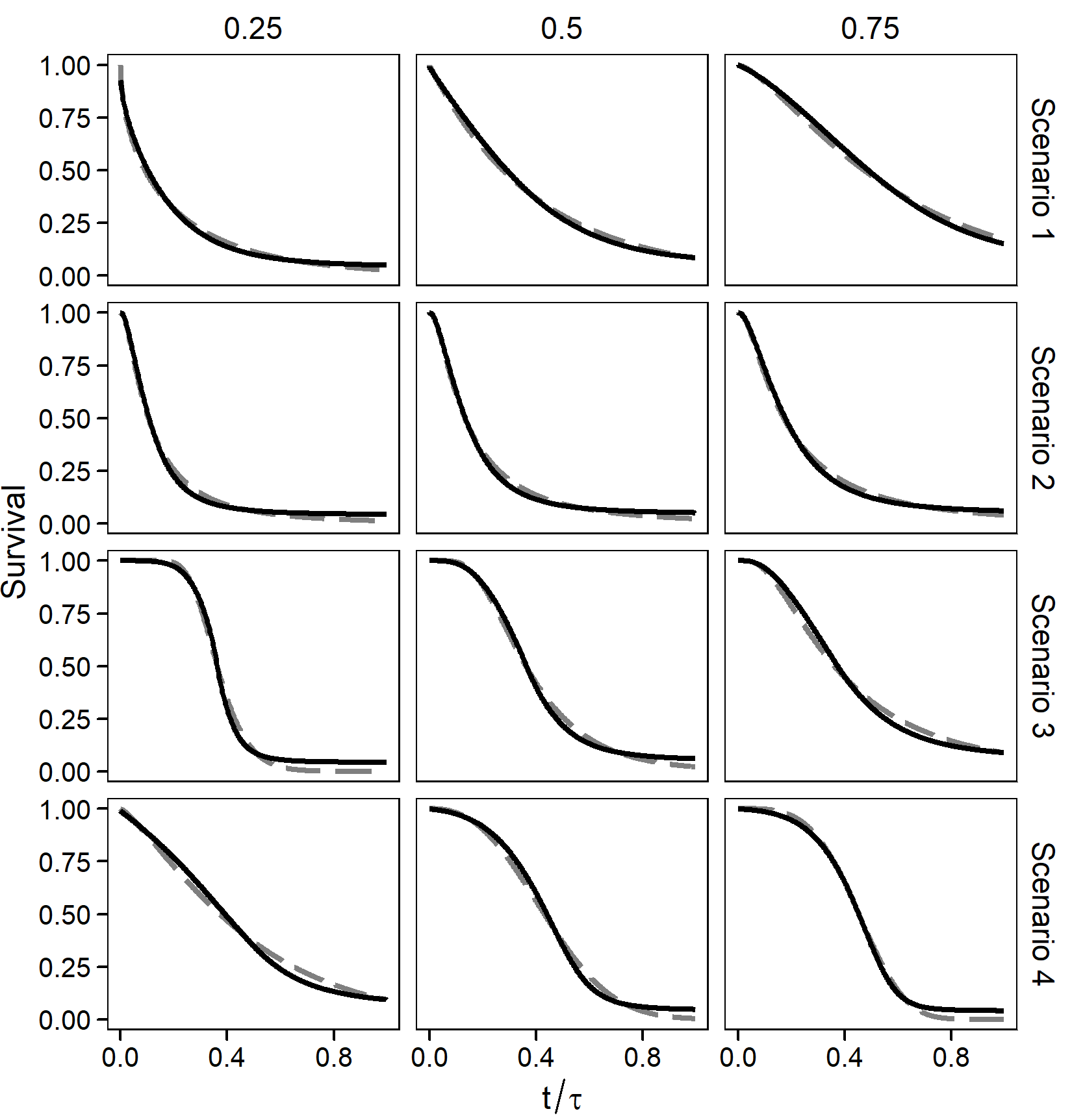
Figure 5: Averaged survival prediction (grey dashes) versus the true lifetime distributions (black solid).

where $\Lambda_{0}(t_{p})$ is the random forest mean cumulative hazard at $t_{p}$, and $\left(\Lambda_{L}^{(r)}(\cdot),\,\Lambda_{U}^{(r)}(\cdot)\right)$ is the confidence band obtained at the $r$th iteration. In the case of our simulations, we have the true distribution for each scenario. However, random forests estimators can be biased (Cui et al., 2019). Given a set of tuning parameters, we do not know the bias theoretically. Hence, we instead approximate the truth $\Lambda_{0}(t_{p})$ using the empirical mean of all $R=1000$ random forest estimators. This empirical mean is indeed very close to the true cumulative hazard function, as we can see from Fig. 5 in the Appendix. The bias is most prominent in the tails, so we would expect the coverage of the truth in earlier time points to be similar to the coverage of the expected random forest. Since potential bias can comprise the validity of the covariate rate estimation, we use this approximation of the mean random forest estimator as the true mean value of the mean cumulative hazard. In the following, we analyze the performance from three aspects: the overall coverage rate, the variance of the proposed estimator, and the effect of the number of trees.

4.2 Coverage Rates

Table 2 summarizes the coverage probabilities for the $95\%$ confidence bands obtained by two covariance matrix correction methods under different scenarios. Original projection means only projecting $\hat{\Sigma}$ to the nearest positive definite matrix $\hat{\Sigma}^{(+)}$ without smoothing correction, while smoothed projection means combining projection and smoothing corrections. We can see that the original projection method has slightly lower coverage probabilities than the target of $95\%$. In contrast, the confidence bands constructed by the smoothed projection method included the random forest truth in at least $95\%$ of the simulations for every scenario. These results show the power of our proposed methodology for producing functioning confidence bands.

Table 2: The coverage probabilities for the $95\%$ confidence bands of the cumulative risk functions at different values of $x_{i}=(x_{i}^{(1)},\,0.50,\,\ldots,\,0.50)^{T}$ under different scenarios.

	$x_{i}^{(1)}$	Original Projection	Smoothed Projection
Scenario 1	0.25	0.913	0.954
	0.50	0.947	0.977
	0.75	0.944	0.976
Scenario 2	0.25	0.884	0.971
	0.50	0.898	0.981
	0.75	0.869	0.981
Scenario 3	0.25	0.901	0.967
	0.50	0.921	0.981
	0.75	0.871	0.968
Scenario 4	0.25	0.940	0.972
	0.50	0.943	0.981
	0.75	0.930	0.974

To identify the time points that tend to fall out of the confidence bands, we provide Fig. 1, which gives the pointwise coverage probabilities over time based on the original projection and the smoothed projection correction methods. A y-axis limit of $0.97\leq y\leq 1$ is used for a simplified presentation, which cuts off some time points in Scenarios 2 and 3, the log-Normal scenarios. Because the critical value we choose, $\zeta_{\alpha}$, is based on the entire cumulative risk curve and not a single point, the pointwise coverage probabilities are much higher than the nominal level $\alpha=95\%$. The lowest pointwise coverage is for Scenario 2, where the original projection covers only 0.94 at $t=0.01\tau$ when $x^{(1)}=0.75$. The original projection method shows its weakness at many earlier time points with sharp drops in Scenarios 2 and 3. The smoothed projection method prevents abrupt changes, and the pointwise coverage probabilities are almost always better than that of the original projection method. The weaker performance for the smoothed projection method is in the middle time points, with both tails having pointwise coverage probabilities over $99\%$. However, the smoothed projection method has nearly perfect pointwise coverage probabilities in the later time points for some of the scenarios, one possible reason for which we will discuss in section 4.3.

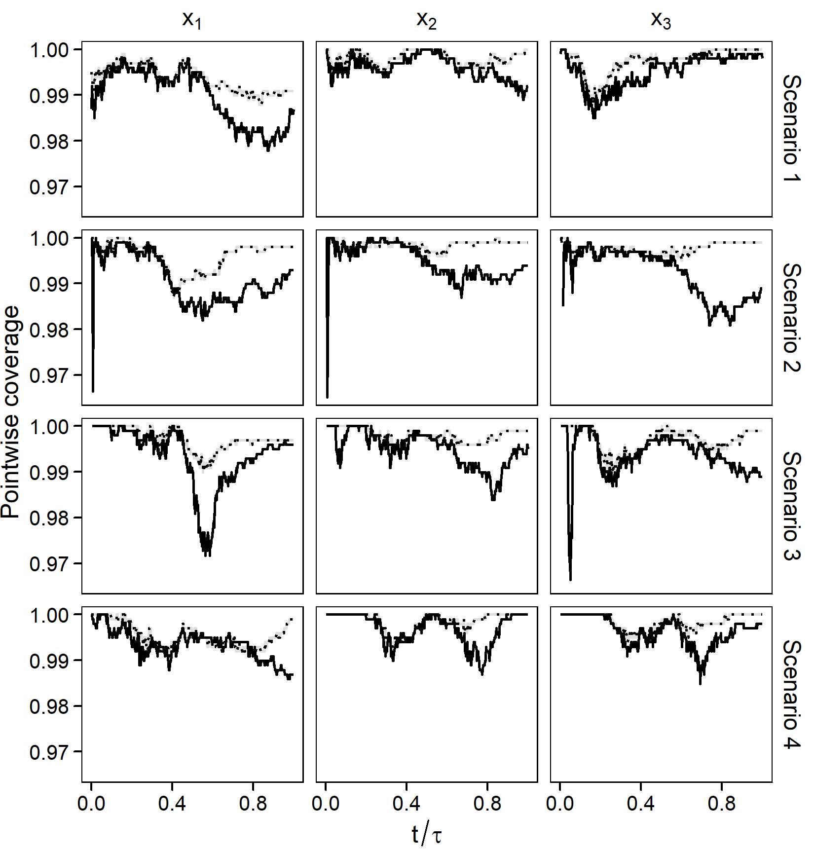
Figure 1: Pointwise coverage probabilities obtained by the original projection method (solid) and the smoothed projection method (dots) over time.

4.3 Marginal Variance Analysis

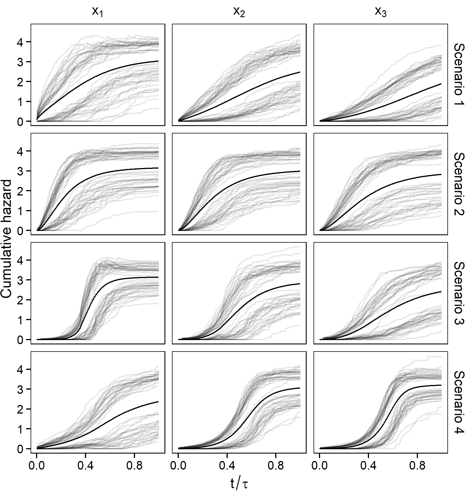
Figure 6: For each scenario, 25 confidence bands constructed by smoothed projection method (grey) and the true cumulative hazard function (black).

First, we present a randomly selected 25 confidence bands constructed by the smoothed projection method for each scenario to demonstrate their variations. These results are shown in Fig. 6 in the Appendix. There are cases where the bands came close to excluding the random forest truth, but there are very few bounds that cross the random forest truth. Scenario 2 has the most simulations in this visual that are very close or fail to contain the truth, but it still achieves good coverage.

Furthermore, we compare two corrections of the covariance matrix: the original and smoothed projections. The primary problem with estimating the marginal variance is that some estimates are negative values. In our simulation, the proportion of negative marginal variances for these scenarios ranged from approximately $0.1\%$ (Scenario 1 when the target point is $x_{1}$) to 8.2% (Scenario 2 when the target point is $x_{1}$).

Figure 2 shows the process of the corrections. The left plot shows the original marginal variance estimators from 25 simulations in Scenario 1, some of which are negative. The middle plot gives the marginal variances from the same simulations after projection. The negative variance estimators in the left plot have been corrected. The marginal variances are visually almost identical except for the negative marginal variances. The right plot shows the estimation results combining projection and smoothing, which cleans up some of the sharp drops and spikes in the variance estimations.

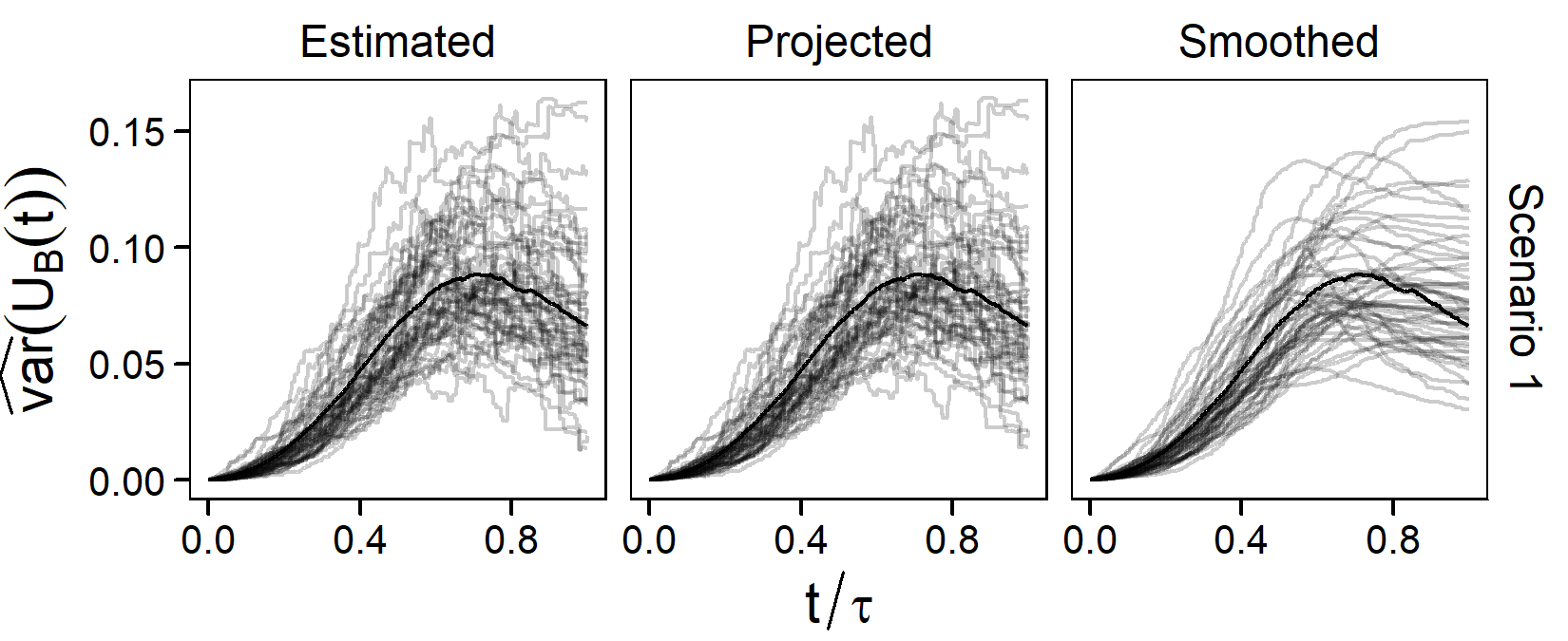
Figure 2: Two-step correction procedure for the marginal variance of 25 simulations (grey) in Scenario 1. From left to right: original marginal variances, projected marginal variances, and final estimated marginal variances after projection and smoothing. True marginal variance in black.

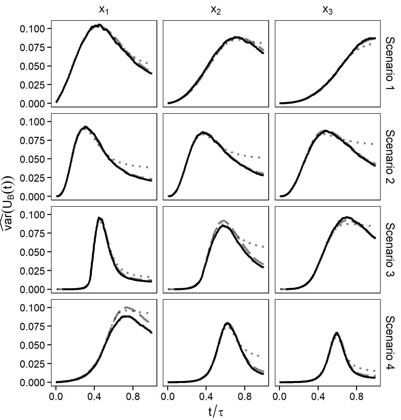
Figure 7: A comparison of the average estimated variances calculated by the original projection method (dashed grey) and the smoothed projection method (dotted grey) with the true variance (solid black).

Next, we examine how close the estimated marginal variances are to the actual marginal variance of random forest predictions. To find the actual variance of the random forest predictions, we calculate the marginal variance at time $t_{p}$ by calculating the sample variance of the random forest predictions at time $t_{p}$ across all simulations. Figure 7 compares the sample variance curve overall simulations to the average of the estimated variances across all simulation runs. Except for $x_{1}$ in Scenario 4, the initially projected variance closely tracks the truth. The smoothed projected variance also closely follows the actual variance at earlier time points. However, the smoothed projected variance is biased at later time points and, in most cases, overestimates the true variance. This bias leads to over-coverage at later time points and the nearly 100% coverage in Fig. 1. Although smoothing introduces bias, it does bring the overall coverage probabilities in Table 2 to the desired level. Therefore, we still prefer the smoothed projected variance.

4.4 Number of Trees and Negative Variance

Our final analysis shows the effect of the number of trees, $B$, for estimating the marginal variance. Focusing on Scenario 3, we re-ran the above analysis with several different values of $B$. The coverage probabilities of the estimated confidence bands and the average proportions of negative estimated marginal variances in $\hat{\Sigma}$ before projection are listed in Table 3, while the point-wise proportion is plotted in Fig. 3(a). Fig. 3(b) shows the sample variance of the estimated marginal variance from $\hat{\Sigma}^{(+)}$.

Table 3: The coverage and proportions of negative estimated marginal variances under different numbers of trees.

	Proportion of Negative Variance			Coverage Probability
$B$	$x^{(1)}$=0.25	$x^{(1)}$=0.5	$x^{(1)}$=0.75	$x^{(1)}$=0.25	$x^{(1)}$=0.5	$x^{(1)}$=0.75
500	0.250	0.147	0.139	0.960	0.97	0.950
1,000	0.198	0.114	0.070	0.960	0.96	0.980
2,500	0.097	0.049	0.036	0.940	0.97	0.960
5,000	0.074	0.026	0.014	0.920	0.95	0.980
10,000	0.036	0.008	0.005	0.949	0.98	0.939
20,000	0.022	0.004	0.003	0.990	0.97	0.950

Firstly, as shown in Table 3 and Fig. 3, a smaller number of trees leads to a higher proportion of negative estimated marginal variances. Both Fig. 3(a) and Fig. 3(b) are loess smoothed with a span of 0.2 for clearer display of the trend. In Fig. 3(b), the smaller the number of trees, the further the line is from 0, which implies that the smaller number of trees, the more variable the estimated marginal variance is. The highest proportion of negative variances and the most variable estimates are for $B=500$. This number is much smaller than generally recommended for random survival forests, so it is not surprising that it performs poorly on both metrics. There is a significant drop in the proportion of negative variances between $B=5,000$ and $B=10,000$. The setting we used for the simulations in Section 4.1 is the second lightest line ($B=10,000$), with a low proportion of negative estimated marginal variances and a relatively stable estimator. Although the darkest line ($B=20,000$) shows the best result, the difference between these two in either metric is not much. Therefore, we used $B=10,000$ for the above simulations.

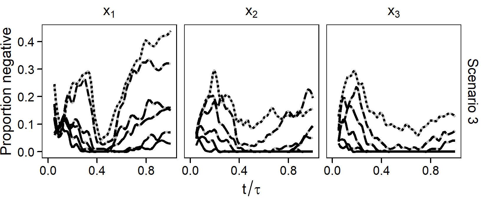
(a) The pointwise proportions of negative estimated marginal variances.

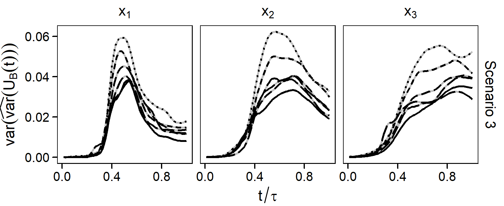
(b) Variance of $\hat{\text{var}}(U_{B}(t))$ by number of trees.

Figure 3: Lines for $B=500,\,1,000,\,2,500,\,5,000,\,10,000$ and $20,000$, ascending in density of points with $B=500$ as single points and $B=20,000$ as a solid line.

Even with high proportions of initial negative marginal variances, our methodology manages almost 95% confidence without significant over-coverage caused by variance overestimation in the right tail.

5 Real Data Analysis

We further demonstrated our method using a data set from Kalbfleisch and Prentice (1980) on veteran’s administration lung cancer data. This data is also used in Ishwaran et al. (2008). The data is available in the R package randomForestSRC (Ishwaran and Kogalur, 2022) as veteran. The response variable $y$ is days of survival. In the case of a subject dropping out of the study, $y$ is the days until drop-out. $n=137$ subjects had measurements for six predicted variables and a recorded death or last follow-up time. 6.6% of the response times were censored.

We ran a random forest with the best split, a minimum terminal node size of 5, and 3 for the number of variables considered at each split. Based on this result, subjects 88 and 97 were selected as our test subjects to demonstrate their different predicted out-of-bag survival curves. We re-ran the random forest without those two subjects and calculated the estimated covariance matrices and confidence bands.

The confidence bands in Fig. 4 are significantly different between the two subjects. Subject 88 was a 51-year-old with squamous lung cancer diagnosed two months before the study began and had a good Karnofsky performance score. His relatively long survival time of $y=283$ matches the slowly increasing cumulative hazard prediction and bands. The marginal variance keeps growing over time, showing a much wider range of possible cumulative hazard values at later time points. Subject 97, on the other hand, was a 66-year-old with small cell lung cancer diagnosed 11 months before the study and had a poor Karnofsky performance score. His short survival time of $y=7$ matches a much quicker increase in the cumulative hazard prediction and bands. The marginal variance stabilizes, and the prediction gives a consistent cumulative hazard range over time.

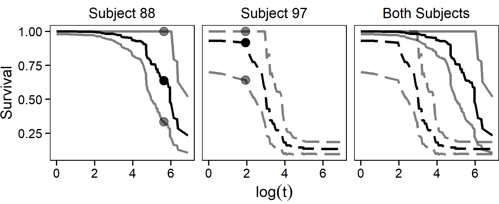
Figure 4: Estimated survival curves (black) and confidence bands (grey) for test subjects 97 (dots) and 88 (dashes). Actual survival time marked with a solid point.

6 Discussion

We proposed a theoretically valid and unbiased confidence band estimator of random survival forests. This addresses the vacancy in the current literature. We also did not address the ratio consistency or rate of convergence of the covariance estimation since existing theory does not seem to provide enough tools or understanding of the $k=O(n)$ scenario. These theoretical considerations should be analyzed in the future.

Our method can be extended in several different directions. For example, the variable importance measure of a random survival forest is often done by calculating the C-index. However, these measures do not have appropriate associated confidence intervals, making inference difficult. As another direction, Xu et al. (2022) considers $k>n/2$ for regression random forests using bootstrap approximations of the true variance. This can be incorporated into our approach if the bootstrap estimation is accurate. Thirdly, our process for handling the non-positive definiteness and choosing a critical value may benefit from projection to a particular form of a covariance matrix that would lead to a more direct critical value choice. We could use theory on a specific type of covariance matrix, such as assuming an autoregressive covariance matrix. The addition of smoothing along the diagonal of the covariance matrix, while it improves the summary metrics, also introduces a bias and slight over-coverage to the right tail. We could also consider an off-diagonal correction after smoothing.

Appendix 1

Proofs

of Theorem 1.

For the fixed $t_{1}$ and $t_{2}$, the covariance of an order-$k$ complete U-statistics is

$$\text{cov}\{U(t_{1}),\,U(t_{2})\}= \binom{n}{k}^{-1}\binom{n}{k}^{-1}\sum_{S_{i}\subset{\cal D}_{n}}\sum_{S_{j}\subset{\cal D}_{n}}\text{cov}\Big{\{}h(t_{1};\,S_{i}),\,h(t_{2};\,S_{j})\Big{\}}$$

$$= \binom{n}{k}^{-2}\sum_{d=1}^{k}\sum_{\mid S_{i}\cap S_{j}\mid=d}\text{cov}\Big{\{}h(t_{1};\,S_{i}),\,h(t_{2};\,S_{j})\Big{\}}.$$

For a pairs of subsamples $S_{i}$ and $S_{j}$ with $d$ overlapping samples, let

$$\xi_{d,\,k}^{2}(t_{1},\,t_{2})=\text{cov}\Big{\{}h(t_{1};\,S_{i}),\,h(t_{2};\,S_{j})\Big{\}}.$$

Then we have

$$\xi_{d,\,k}^{2}(t_{1},\,t_{2})= \text{cov}\Big{[}E\{h(t_{1};\,S)\mid Z_{(1:d)}\},\,E\{h(t_{2};\,S)\mid Z_{(1:d)}\}\Big{]}$$

$$= \text{cov}\Big{\{}h(t_{1};\,S),\,h(t_{2};\,S)\Big{\}}-E\Big{[}\text{cov}\{h(t_{1};\,S),\,h(t_{2};\,S)\mid Z_{(1:d)}\}\Big{]}.$$

Denote

$$\tilde{\xi}_{d,\,k}^{2}(t_{1},\,t_{2})=E\Big{[}\text{cov}\{h(t_{1};\,S),\,h(t_{2};\,S)\mid Z_{(1:d)}\}\Big{]},$$

then

$$\xi_{d,\,k}^{2}(t_{1},\,t_{2})=\text{cov}\Big{\{}h(t_{1};\,S),\,h(t_{2};\,S)\Big{\}}-\tilde{\xi}_{d,\,k}^{2}(t_{1},\,t_{2}),$$

hence

$$\text{cov}\{U(t_{1}),\,U(t_{2})\}= \binom{n}{k}^{-2}\sum_{d=1}^{k}\sum_{\mid S_{i}\cap S_{j}\mid=d}\xi_{d,\,k}^{2}(t_{1},\,t_{2})$$

$$= \binom{n}{k}^{-2}\sum_{d=1}^{k}\binom{n}{k}\binom{k}{d}\binom{n-k}{k-d}\xi_{d,\,k}^{2}(t_{1},\,t_{2})$$

$$= \binom{n}{k}^{-1}\sum_{d=1}^{k}\binom{k}{d}\binom{n-k}{k-d}\left[\text{cov}\big{\{}h(t_{1};\,S),\,h(t_{2};\,S)\big{\}}-\tilde{\xi}_{d,\,k}^{2}(t_{1},\,t_{2})\right]$$

$$= \sum_{d=1}^{k}\gamma_{d,k,n}\left[\text{cov}\big{\{}h(t_{1};\,S),\,h(t_{2};\,S)\big{\}}-\tilde{\xi}_{d,\,k}^{2}(t_{1},\,t_{2})\right]$$

$$= (1-\gamma_{0,k,n})\,\text{cov}\big{\{}h(t_{1};\,S),\,h(t_{2};\,S)\big{\}}-$$

$$\left\{\sum_{d=0}^{k}\gamma_{d,k,n}\,\tilde{\xi}_{d,\,k}^{2}(t_{1},\,t_{2})-\gamma_{0,k,n}\,\tilde{\xi}_{0,\,k}^{2}(t_{1},\,t_{2})\right\}$$

$$= \text{cov}\big{\{}h(t_{1};\,S),\,h(t_{2};\,S)\big{\}}-\sum_{d=0}^{k}\gamma_{d,k,n}\,\tilde{\xi}_{d,\,k}^{2}(t_{1},\,t_{2})$$

$$= C^{(h)}(t_{1},t_{2})-C^{(S)}(t_{1},\,t_{2}).$$

To estimate $C^{(h)}(t_{1},\,t_{2})$, we use the fact that

$$C^{(h)}(t_{1},\,t_{2})= \text{cov}\Big{\{}h(t_{1};\,S),\,h(t_{2};\,S)\Big{\}}$$

$$= E\left[\frac{1}{2}\{h(t_{1};\,S_{i})-h(t_{1};\,S_{j})\}\{h(t_{2};\,S_{i})-h(t_{2};\,S_{j})\}\right]$$

where the pair of $S_{i}$ and $S_{j}$ does not contain any overlapping samples, hence $C^{(h)}(t_{1},t_{2})$ can also be estimated as

$$\hat{C}^{(h)}(t_{1},\,t_{2})=\frac{1}{2N_{0}}\sum_{S_{i}\cap S_{j}=\emptyset}\Big{\{}h(t_{1};\,S_{i})-h(t_{1};\,S_{j})\Big{\}}\Big{\{}h(t_{2};\,S_{i})-h(t_{2};\,S_{j})\Big{\}}.$$

To estimate $C^{(S)}(t_{1},\,t_{2})$, we need to deal with $\text{cov}\{h(t_{1};\,S),\,h(t_{2};\,S)\mid Z_{(1:d)}\}$ first. For a pair of subsamples $S_{i}$ and $S_{j}$ such that $S_{i}\cap S_{j}=Z_{(1:d)}$,

$$\text{cov}\big{\{}h(t_{1};\,S),\,h(t_{2};\,S)\mid Z_{(1:d)}\big{\}}=E\left[\frac{1}{2}\{h(t_{1};\,S_{i})-h(t_{1};\,S_{j})\}\{h(t_{2};\,S_{i})-h(t_{2};\,S_{j})\}\right],$$

hence $\tilde{\xi}_{d,\,k}^{2}(t_{1},\,t_{2})$ can be estimated by all such pairs of subsamples,

$$\hat{\tilde{\xi}}_{d,\,k}^{2}(t_{1},\,t_{2})=\frac{1}{N_{d}}\sum_{\mid S_{i}\cap S_{j}\mid=d}\frac{1}{2}\{h(t_{1};\,S_{i})-h(t_{1};\,S_{j})\}\{h(t_{2};\,S_{i})-h(t_{2};\,S_{j})\},$$

where

$$N_{d}=\binom{n}{k}\binom{k}{d}\binom{n-k}{k-d}$$

is the number of the pairs with $d$ overlapping samples. Then

$$\hat{C}^{(S)}(t_{1},\,t_{2})= \sum_{d=0}^{k}\gamma_{d,k,n}\,\tilde{\xi}_{d,\,k}^{2}(t_{1},\,t_{2})$$

$$= \sum_{d=0}^{k}\gamma_{d,k,n}\left[\frac{1}{N_{d}}\sum_{\mid S_{i}\cap S_{j}\mid=d}\frac{1}{2}\,\{h(t_{1};\,S_{i})-h(t_{1};\,S_{j})\}\{h(t_{2};\,S_{i})-h(t_{2};\,S_{j})\}\right]$$

$$= \sum_{d=0}^{k}\binom{n}{k}^{-2}\sum_{\mid S_{i}\cap S_{j}\mid=d}\frac{1}{2}\,\{h(t_{1};\,S_{i})-h(t_{1};\,S_{j})\}\{h(t_{2};\,S_{i})-h(t_{2};\,S_{j})\}$$

$$= \underbrace{\binom{n}{k}^{-2}}_{\text{number of pairs}}\underbrace{\sum_{d=0}^{k}\sum_{\mid S_{i}\cap S_{j}\mid=d}}_{\text{all pairs of $k$ samples}}\frac{1}{2}\,\{h(t_{1};\,S_{i})-h(t_{1};\,S_{j})\}\{h(t_{2};\,S_{i})-$$

$$h(t_{2};\,S_{j})\}$$

$$= \binom{n}{k}^{-2}\sum_{S_{i}\neq S_{j}}\frac{1}{2}\,\{h(t_{1};\,S_{i})-h(t_{1};\,S_{j})\}\{h(t_{2};\,S_{i})-h(t_{2};\,S_{j})\}.$$

This term can be estimated by using all of the $k$ data subsample $S_{i}$,

$$\hat{C}^{(S)}(t_{1},\,t_{2})=\frac{1}{N}\sum_{S_{i}\subset{\cal D}_{n}}\{h(t_{1};\,S_{i})-U(t_{1})\}\{h(t_{2};\,S_{i})-U(t_{2})\}.$$

∎

of Theorem 2.

For given $t_{1}$ and $t_{2}$, the difference between $\text{cov}\{U_{B}(t_{1}),\,U_{B}(t_{2})\}$ and its complete counterpart $\text{cov}\{U(t_{1}),\,U(t_{2})\}$ is

$$E\Big{[}\text{cov}\{U_{B}(t_{1}),\,U_{B}(t_{2})\mid{\cal D}_{n}\}\Big{]}= E\Big{[}E\{U_{B}(t_{1})U_{B}(t_{2})\mid{\cal D}_{n}\}-E\{U_{B}(t_{1})\mid{\cal D}_{n}\}E\{U_{B}(t_{2})\mid{\cal D}_{n}\}\Big{]}$$

$$= E\Big{[}E\{U_{B}(t_{1})U_{B}(t_{2})\mid{\cal D}_{n}\}-U(t_{1})U(t_{2})\Big{]}.$$ (9)

The first item in the above equation is

$$E\{U_{B}(t_{1}) U_{B}(t_{2})\mid{\cal D}_{n}\}$$

$$= E\left(\frac{1}{4B^{2}}\left[\sum_{b=1}^{B}\{h(t_{1};\,S_{b1})+h(t_{1};\,S_{b2})\}\right]\left[\sum_{b=1}^{B}\{h(t_{2};\,S_{b1})+h(t_{2};\,S_{b2})\}\right]\mid{\cal D}_{n}\right)$$

$$= \frac{1}{4B^{2}}\sum_{b=1}^{B}E\left[\left\{h(t_{1};\,S_{b1})+h(t_{1};\,S_{b2})\right\}\left\{h(t_{2};\,S_{b1})+h(t_{2};\,S_{b2})\right\}\mid{\cal D}_{n}\right]$$

$$+\frac{2}{4B^{2}}\sum_{b1<b2}E\left[\left\{h(t_{1};\,S_{b1,1})+h(t_{1};\,S_{b1,2})\right\}\left\{h(t_{2};\,S_{b2,1})+h(t_{2};\,S_{b2,2})\right\}\mid{\cal D}_{n}\right]$$

$$\doteq\text{Part I}+\text{Part II}.$$

We have

$$\text{Part I}= \frac{1}{4B^{2}}\sum_{b=1}^{B}E\Big{\{}h(t_{1};\,S_{b1})h(t_{2};\,S_{b1})+h(t_{1};\,S_{b2})h(t_{2};\,S_{b2})$$

$$\qquad\qquad\qquad+h(t_{1};\,S_{b1})h(t_{2};\,S_{b2})+h(t_{1};\,S_{b2})h(t_{2};\,S_{b1})\mid{\cal D}_{n}\Big{\}}$$

$$= \frac{2}{4B^{2}}\sum_{b=1}^{B}E\left\{h(t_{1};\,S_{b1})h(t_{2};\,S_{b1})\mid{\cal D}_{n}\right\}+\frac{2}{4B^{2}}\sum_{b=1}^{B}E\left\{h(t_{1};\,S_{b1})h(t_{2};\,S_{b2})\mid{\cal D}_{n}\right\}$$

$$= \frac{1}{2\,B\,N}\sum_{S_{i}\subset{\cal D}_{n}}h(t_{1};\,S_{i})h(t_{2};\,S_{i})+\frac{1}{2\,B\,N\,\binom{n-k}{k}}\sum_{S_{i}\cap S_{j}=\emptyset}h(t_{1};\,S_{i})\,h(t_{2};\,S_{j}).$$

Since

$$\sum_{S_{i}\cap S_{j}=\emptyset}\left\{h(t_{1};\,S_{i})+h(t_{1};\,S_{j})\right\}\left\{h(t_{2};\,S_{i})+h(t_{2};\,S_{j})\right\}$$

$$= \binom{n-k}{k}\sum_{S_{i}\subset{\cal D}_{n}}2\,h(t_{1};\,S_{i})h(t_{2};\,S_{i})+2\sum_{S_{i}\cap S_{j}=\emptyset}h(t_{1};\,S_{i})h(t_{2};\,S_{j}),$$

we get

$$\text{Part I}= \frac{1}{2BN}\sum_{S_{i}\subset{\cal D}_{n}}h(t_{1};\,S_{i})\,h(t_{2};\,S_{i})-\frac{1}{2BN}\sum_{S_{i}\subset{\cal D}_{n}}h(t_{1};\,S_{i})h(t_{2};\,S_{j})$$

$$\quad+\frac{1}{4BN\binom{n-k}{k}}\sum_{S_{i}\cap S_{j}=\emptyset}\left\{h(t_{1};\,S_{i})-h(t_{1};\,S_{j})\right\}\left\{h(t_{2};\,S_{i})-h(t_{2};\,S_{j})\right\}$$

$$= \frac{1}{4BN\binom{n-k}{k}}\sum_{S_{i}\cap S_{j}=\emptyset}\left\{h(t_{1};\,S_{i})+h(t_{1};\,S_{j})\right\}\left\{h(t_{2};\,S_{i})+h(t_{2};\,S_{j})\right\}.$$

The second term of (of Theorem 2.) is

$$\text{Part II}= \frac{1}{B^{2}}\sum_{1\leq b2<b2\leq B}E\left[h(t_{1};\,S_{b1,1})\left\{h(t_{2};\,S_{b2,1})+h(t_{2};\,S_{b2,2})\right\}\mid{\cal D}_{n}\right]$$

$$= \frac{B-1}{2B}\,E\left[h(t_{1};\,S_{11})\left\{h(t_{2};\,S_{21})+h(t_{2};\,S_{22})\right\}\mid{\cal D}_{n}\right]$$

$$= \frac{B-1}{2B}\frac{1}{N^{2}\binom{n-k}{k}}\sum_{\genfrac{}{}{0.0pt}{}{i,\,j,\,j^{\prime}}{S_{j}\cap S_{j^{\prime}}=\emptyset}}h(t_{1};\,S_{i})\left\{h(t_{2};\,S_{j})+h(t_{2};\,S_{j^{\prime}})\right\}$$

$$= \frac{B-1}{2B}\frac{1}{N^{2}\binom{n-k}{k}}\{\sum_{i,\,j}\sum_{j^{\prime}:\,S_{j}\cap S_{j^{\prime}}=\emptyset}\,h(t_{1};\,S_{i})h(t_{2};\,S_{j})$$

$$+\sum_{i,\,j^{\prime}}\sum_{j:\,S_{j}\cap S_{j^{\prime}}=\emptyset}\,h(t_{1};\,S_{i})h(t_{2};\,S_{j^{\prime}})\}$$

$$= \frac{B-1}{2B}\frac{1}{N^{2}}\left\{\sum_{i,\,j}\,h(t_{1};\,S_{i})h(t_{2};\,S_{j})+\sum_{i,\,j^{\prime}}\,h(t_{1};\,S_{i})h(t_{2};\,S_{j^{\prime}})\right\}$$

$$= \left(1-\frac{1}{B}\right)\left\{\frac{1}{N}\sum_{S_{i}\subset{\cal D}_{n}}h(t_{1};\,S_{i})\right\}\left\{\frac{1}{N}\sum_{S_{i}\subset{\cal D}_{n}}h(t_{2};\,S_{i})\right\}$$

Hence

$$\text{cov}\{U_{B}(t_{1}), \,U_{B}(t_{2})\mid{\cal D}_{n}\}=\text{Part I}+\text{Part II}-U(t_{1})\,U(t_{2})$$ (10)

$$= \frac{1}{4BN\binom{n-k}{k}}\sum_{S_{i}\cap S_{j}=\emptyset}\left\{h(t_{1};\,S_{i})+h(t_{1};\,S_{j})\right\}\left\{h(t_{2};\,S_{i})+h(t_{2};\,S_{j})\right\}$$

$$-\frac{1}{B}\,U(t_{1})\,U(t_{2})$$

Therefore the difference between $\text{cov}\{U_{B}(t_{1}),\,U_{B}(t_{2})\}$ and $\text{cov}\{U(t_{1}),\,U(t_{2})\}$ is

$$E\Big{[}\text{cov}\{U_{B}(t_{1}),\,U_{B}(t_{2})\mid{\cal D}_{n}\}\Big{]}= \frac{1}{4B}\,E[\{h(t_{1};\,S_{i})+h(t_{1};\}\{h(t_{2};\,S_{i})$$

$$+h(t_{2};\,S_{j})\}]-\frac{1}{B}\,E\{\,U(t_{1})U(t_{2})\}$$

$$= \frac{1}{2B}\Big{[}E\{\,h(t_{1};\,S)h(t_{2};\,S)\}+E\{\,h(t_{1};\,S)\,E\,h(t_{2};\,S)\}$$

$$-2\,E\{\,U(t_{1})U(t_{2})\}\Big{]}$$

$$= \frac{1}{2B}\Big{[}\text{cov}\{h(t_{1};\,S),\,h(t_{2};\,S)\}-2\,\text{cov}\{U(t_{1}),\,U(t_{2})\}\Big{]}$$

$$= \frac{1}{2B}C^{(h)}(t_{1},\,t_{2})-\frac{1}{B}\text{cov}\{U(t_{1}),\,U(t_{2})\}.$$

Hence we get the result. ∎

of Theorem 3.

Since

$$\hat{C}^{(S)}_{B}(t_{1},\,t_{2})= \frac{1}{2B}\sum_{b=1}^{B}\Big{[}h(t_{1};\,S_{b1})h(t_{2};\,S_{b1})+h(t_{1};\,S_{b2})h(t_{2};\,S_{b2})+2U_{B}(t_{1})U_{B}(t_{2})$$

$$\qquad\qquad-2\{h(t_{2};\,S_{b1})+h(t_{2};\,S_{b2})\}U_{B}(t_{1})-2\{h(t_{1};\,S_{b1})$$

$$\qquad\qquad+h(t_{1};\,S_{b2})\}U_{B}(t_{2})\Big{]}$$

$$= \frac{1}{2B}\sum_{b=1}^{B}\Big{\{}h(t_{1};\,S_{b1})h(t_{2};\,S_{b1})+h(t_{1};\,S_{b2})h(t_{2};\,S_{b2})\Big{\}}-U_{B}(t_{1})U_{B}(t_{2})$$

together with (10), we have

$$E\left\{\hat{C}^{(S)}_{B}(t_{1},\,t_{2})\right\}= E\left[\frac{1}{B}\sum_{b=1}^{B}E\left\{h(t_{1};\,S_{b1})h(t_{2};\,S_{b1})\mid{\cal D}_{n}\right\}\right]$$

$$-E\Big{[}\text{cov}\{U_{B}(t_{1}),\,U_{B}(t_{2})\mid{\cal D}_{n}\}+U(t_{1})U(t_{2})\Big{]}$$

$$= E\left\{\frac{1}{N}\sum_{S_{i}\subset{\cal D}_{n}}h(t_{1};\,S_{i})h(t_{2};\,S_{i})-U(t_{1})U(t_{2})\right\}$$

$$-\frac{1}{B}\left[\frac{1}{2}\,C^{(h)}(t_{1},\,t_{2})-\text{cov}\{U(t_{1}),\,U(t_{2})\}\right]$$

$$= \left[C^{(h)}(t_{1},\,t_{2})-\text{cov}\{U(t_{1}),\,U(t_{2})\}\right]$$

$$-\frac{1}{B}\left[\frac{1}{2}\,C^{(h)}(t_{1},\,t_{2})-\text{cov}\{U(t_{1}),\,U(t_{2})\}\right]$$

$$= \left(1-\frac{1}{B}\right)C^{(S)}(t_{1},\,t_{2})+\frac{1}{2B}\,C^{(h)}(t_{1},\,t_{2}).$$

∎

Appendix 2

Additional Figures

Table 4: D-optimality values for design $X$ under five different scenarios.

one	two	three	four	five
1.23	3.45	5.00	1.21	3.41
1.23	3.45	5.00	1.21	3.42
1.23	3.45	5.00	1.21	3.43

References

- Athey et al. (2019) Athey, S., J. Tibshirani, and S. Wager (2019). Generalized random forests. Annals of Statistics 47(2), 1179–1203.
- Bose and Sen (2002) Bose, A. and A. Sen (2002). Asymptotic distribution of the Kaplan-Meier U-statistics. Journal of Multivariate Analysis 83, 84–123.
- Breiman (2001) Breiman, L. (2001). Random Forests. Machine Learning 45, 5–32.
- Chen et al. (2010) Chen, X., L. Wang, and H. Ishwaran (2010). An integrative pathway-based clinical-genomic model for cancer survival prediction. Statistics and Probability Letters 80(17-18), 1313–1319.
- Conde-Amboage et al. (2021) Conde-Amboage, M., I. Van Keilegom, and W. González-Manteiga (2021). A new lack-of-fit test for quantile regression with censored data. Scandinavian Journal of Statistics 48(2), 655–688.
- Cox (1972) Cox, D. R. (1972). Regression models and life-tables. Journal of the Royal Statistical Society: Series B (Methodological) 34(2), 187–202.
- Cui et al. (2020) Cui, Y., M. R. Kosorok, E. Sverdrup, S. Wager, and R. Zhu (2020). Estimating heterogeneous treatment effects with right-censored data via causal survival forests. arXiv preprint arXiv:2001.09887.
- Cui et al. (2019) Cui, Y., R. Zhu, M. Zhou, and M. Kosorok (2019). Consistency of survival tree and forest models: splitting bias and correction. arXiv.
- Folsom (1984) Folsom, R. E. (1984). Probability sample u-statistics: Theory and applications for complex sample designs. Technical report, North Carolina State University. Dept. of Statistics.
- Geurts et al. (2006) Geurts, P., D. Ernst, and L. Wehenkel (2006). Extremely randomized trees. Machine learning 63(1), 3–42.
- Hall and Wellner (1980) Hall, W. J. and J. A. Wellner (1980). Confidence Bands for a Survival Curve from Censored Data. Biometrika 67(1), 133–143.
- Hoeffding (1948) Hoeffding, W. (1948). A Class of Statistics with Asymptotically Normal Distribution. The Annals of Mathematical Statistics 19(3), 293–325.
- Hothorn et al. (2006) Hothorn, T., P. Bühlmann, S. Dudoit, A. Molinaro, and M. J. Van Der Laan (2006). Survival ensembles. Biostatistics 7(3), 355–373.
- Ishwaran and Kogalur (2022) Ishwaran, H. and U. Kogalur (2022). Fast Unified Random Forests for Survival, Regression, and Classification (RF-SRC). R package version 3.0.2.
- Ishwaran et al. (2008) Ishwaran, H., U. B. Kogalur, E. H. Blackstone, and M. S. Lauer (2008). Random survival forests. The Annals of Applied Statistics 2(3), 841–860.
- Kalbfleisch and Prentice (1980) Kalbfleisch, J. D. and R. Prentice (1980). The statistical analysis of failure time data. New York: Wiley.
- Koul and Ling (2006) Koul, H. L. and S. Ling (2006). Fitting an error distribution in some heteroscedastic time series models. Annals of Statistics 34(2), 994–1012.
- Lee (1990) Lee, A. J. (1990). U-statistics: Theory and Practice. Boca Raton, FL: CRC Press.
- Lin et al. (1994) Lin, D., T. Fleming, and L. Wei (1994). Confidence bands for survival curves under the proportional hazards model. Biometrika, 73–81.
- Mentch and Hooker (2016) Mentch, L. and G. Hooker (2016). Quantifying uncertainty in random forests via confidence intervals and hypothesis tests. Journal of Machine Learning Research 17, 1–41.
- Peng et al. (2019) Peng, W., T. Coleman, and L. Mentch (2019). Asymptotic distributions and rates of convergence for random forests via generalized u-statistics. arXiv preprint arXiv:1905.10651.
- Peng et al. (2021) Peng, W., L. Mentch, and L. Stefanski (2021). Bias, Consistency, and Alternative Perspectives of the Infinitesimal Jackknife. pp. 1–57.
- Sexton and Laake (2009) Sexton, J. and P. Laake (2009). Standard errors for bagged and random forest estimators. Computational Statistics & Data Analysis 53(3), 801–811.
- Shi and Xu (2019) Shi, M. and G. Xu (2019). Development and validation of GMI signature based random survival forest prognosis model to predict clinical outcome in acute myeloid leukemia. BMC Medical Genomics 12(90), 1–16.
- Silverman (1986) Silverman, B. (1986). Density estimation for statistics and data analysis. London: Chapman and Hall.
- Song et al. (2019) Song, L., X.-Y. Wang, and X.-F. He (2019). A 5-gene prognostic combination for predicting survival of patients with gastric cancer. Medical Science Monitor 25, 6213–6220.
- Steingrimsson et al. (2019) Steingrimsson, J. A., L. Diao, and R. L. Strawderman (2019). Censoring unbiased regression trees and ensembles. Journal of the American Statistical Association 114(525), 370–383.
- Takashima et al. (2020) Takashima, Y., A. Kawaguchi, Y. Iwadate, H. Hondoh, J. Fukai, K. Kajiwara, A. Hayano, and R. Yamanaka (2020). MiR-101, miR-548b, miR-554, and miR-1202 are reliable prognosis predictors of the miRNAs associated with cancer immunity in primary central nervous system lymphoma. PLoS ONE 15(2), 1–14.
- Wager (2014) Wager, S. (2014). Asymptotic Theory for Random Forests. arXiv, 1–17.
- Wager and Athey (2018) Wager, S. and S. Athey (2018). Estimation and Inference of Heterogeneous Treatment Effects using Random Forests. Journal of the American Statistical Association 113(523), 1228–1242.
- Wang and Lindsay (2014) Wang, Q. and B. Lindsay (2014). Variance estimation of a general U-statistic with application to cross-validation. Statistica Sinica 24(3), 1117–1141.
- Xu et al. (2022) Xu, T., R. Zhu, and X. Shao (2022). On variance estimation of random forests. arXiv preprint arXiv:2202.09008.
- Zhang et al. (2019) Zhang, Y., J. Xu, J. Hua, J. Liu, C. Liang, Q. Meng, M. Wei, B. Zhang, X. Yu, and S. Shi (2019). A PD-L2-based immune marker signature helps to predict survival in resected pancreatic ductal adenocarcinoma. Journal for ImmunoTherapy of Cancer 7(233), 1–13.
- Zhou et al. (2021) Zhou, Z., L. Mentch, and G. Hooker (2021). V-statistics and variance estimation. Journal of Machine Learning Research 22(287), 1–48.
- Zhu et al. (2002) Zhu, L. X., K. C. Yuen, and N. Y. Tang (2002). Resampling methods for testing a semiparametric random censorship model. Scandinavian Journal of Statistics 29(1), 111–123.
- Zhu and Kosorok (2012) Zhu, R. and M. R. Kosorok (2012). Recursively imputed survival trees. Journal of the American Statistical Association 107(497), 331–340.