Information Fusion: Scaling Subspace-Driven Approaches

Abstract

In this work, we seek to exploit the deep structure of multi-modal data to robustly exploit the group subspace distribution of the information using the Convolutional Neural Network (CNN) formalism. Upon unfolding the set of subspaces constituting each data modality, and learning their corresponding encoders, an optimized integration of the generated inherent information is carried out to yield a characterization of various classes. Referred to as deep Multimodal Robust Group Subspace Clustering (DRoGSuRe), this approach is compared against the independently developed state-of-the-art approach named Deep Multimodal Subspace Clustering (DMSC). Experiments on different multimodal datasets show that our approach is competitive and more robust in the presence of noise.

1 Introduction

Unsupervised learning is a very challenging topic in Machine Learning (ML), and involves the discovery of hidden patterns in data for inference with no prior given labels. Reliable clustering techniques will save time and effort required for classifying/labeling large datasets that might have thousands of observations. Multi-modal data, increasingly in need for complex application problems, have become more accessible with recent advances in sensor technology, and of pervasive use in practice. The plurality of sensing modalities in our applications of interest, provides diverse and complementary information, necessary to capture the salient characteristics of data and secure their unique signature. A principled combination of the information contained in the different sensors and at different scales is henceforth pursued to enhance understanding of the distinct structure of the various classes of data. The objective of this work is to develop a principled multi-modal framework for object clustering in an unsupervised learning scenario. We extract key class-distinct features-signatures from each data modality using a CNN encoder, and we subsequently non-linearly combine those features to generate a discriminative characteristic feature. In so doing, we work on the hypothesis that each data modality is approximated by a Union of low dimensional Subspaces which highlights underlying hidden features. The UoS structure is unveiled by pursuing sparse self-representation of the given data modality. The subsequent aggregation of the multi-modal subspace structures yields a jointly unified characteristic subspace for each class.

1.1 Related Work

Subspace clustering has been introduced as an efficient way for unfolding union of low-dimensional subspaces underlying high dimensional data. Subspace clustering has been extensively studied in computer vision due to the vast availability of visual data as in Elhamifar and Vidal (2013), Favaro et al. (2011), Li and Vidal (2015), and Bian et al. (2018). This paradigm has broadly been adopted in many applications such as image segmentation Yang et al. (2006), image compression Hong et al. (2006), and object clustering Ho et al. (2003). Uncovering the principles and laying out the fundamentals for multi-modal data has become an important topic in research in light of many applications in diverse fields including image fusion Hellwich and Wiedemann (2000), target recognition Korona and Kokar (1996), Ghanem et al. (2018), Ghanem et al. (2021), Wang et al. (2018), speaker recognition Soong and Rosenberg (1988), and handwriting analysis Xu et al. (1992). Convolutional neural networks have been widely used on multi-modal data as in Ngiam et al. (2011) Ramachandram and Taylor (2017), Valada et al. (2016), Roheda et al. (2018b), and Roheda et al. (2018a). A very similar approach for multi-modal subspace clustering was proposed in Zhu et al. (2019). However, we note and maintain that our formulation results in a different optimization problem, as the multi-modal sensing seeks to not only account for the private information which provides the complementarity of the sensors, but also the common and hidden information. This yields, naturally, to a different network structure than that of Zhu et al. (2019) in a different application space. In addition, the robustness of fusing multi-modal sensor data each with its distinct intrinsic structure, is addressed along with a potential scaling for viability. A thorough comparison of our results to the state of the art multimodal fusion network Abavisani and Patel (2018) is carried out, with a demonstration of resilient fusion under a variety of limiting scenarios including limited sensing modalities (sensor failures).

1.2 Contributions

Building on the work of Deep Subspace Clustering (DSC) Ji et al. (2017), we propose a new and principled multi-modal fusion approach which accounts for a sensor’ capacity to house private and unique information about some observed data as well as that information which is likely also captured and hence common to other sensors. This is accounted for in our robust fusion formulation for multi-modal sensor data. Unveiling the complex UoS of multi-modal data also requires us to account for scaling in our proposed formulation and solution, which in turn invokes the learning of multiple/deep scale Convolutional Neural Networks (CNN). Our proposed Multi-modal fusion approach, by virtue of each sensor information structure (i.e. private plus shared) seeks to enhance and robustify the subspace approximation of shared information for each of the sensors, thus yielding a parallel bank of UoS for each of the sensors. The robust Deep structure effectively achieves scaling while securing structured representation for unsupervised inference. We compare our approach to a well-known deep multimodal network Abavisani and Patel (2018) which was also based on Ji et al. (2017).

In our proposed approach, we thus define the latent space in a way that safeguards the individual sensor private information which hence dedicates more degrees of freedom to each of the sensors. In contrast to the approach in Abavisani and Patel (2018). In our evaluation, we use two recently released data sets each of which we partition into learning and validation subsets. The learned UoS structure for each of the data sets is then utilized to classify new observed data points, which illustrates the generalization power of the proposed approach. Different scenarios with corresponding additive noise to either the training set or the testing set, or both, were used to thoroughly investigate the robustness, and resilience of the clustering approach performance. Experimental results confirm a significant improvement for our Deep Robust Group Subspace Recovery network (DRoGSuRe) under numerous limiting scenarios and demonstrate robustness under these conditions.

The balance of the paper is organized as follows, in Section 2, we provide the problem formulation, background along with the derivation for our proposed approach, Deep Robust Group Subspace Recovery (DRoGSuRe). In Section 3, we describe the attributes of the proposed approach and contrast it to Deep Multimodal Subspace Clustering algorithm (DMSC). In Section 4 and 5, we present a substantiative validation along with experimental results of our approach, while Section 6 provides concluding remarks.

2 Deep Robust Group Subspace Clustering

2.1 Problem Formulation

We assume having a set of data observations, each represented as a $m-$dimensional vector $\mathbf{x_{k}}(t)\in\mathbb{R}^{m}$, where k = 1, 2, …, n. Moreover, we consider having T data modalities, indexed by t = 1, 2, 3, …, T. Each data modality can then be described as $\mathbf{X}(t)=[\mathbf{x}_{1}(t)\ \mathbf{x}_{2}(t)\ ...\ \mathbf{x}_{n}(t)]$. Our objective is to assign each set of data observations into clusters that can be efficiently represented by a low-dimensional subspace. This is equivalent to finding a partitioning {$\mathbf{X}^{1}(t),\mathbf{X}^{2}(t),...,\mathbf{X}^{P}(t)$} of [$n$] observations, where $P$ is the total number of clusters underlying each data modality indexed by $p$. Furthermore, each linear subspace can be described as $\mathbf{S}^{p}(t)\subset\mathbb{R}^{m}$ with dim($\mathbf{S}^{p}(t)$) $\ll m$.
We will exploit the self-expressive property presented in Elhamifar and Vidal (2013) and Bian and Krim (2015), which entails that each data observation $\mathbf{x}_{i}(t)$ can be represented as a linear combination of all features from the same subspace $S(\mathbf{x}_{i}(t))$ as follows,

$$\mathbf{x}_{i}(t)=\sum_{i\neq j,\mathbf{x}_{j}(t)\in S(\mathbf{x}_{i}(t))}w_{ij}(t)\mathbf{x}_{j}(t)$$ (1)

If we stack all the data points $\mathbf{x}_{i}(t)$ into columns of the data matrix $\mathbf{X}(t)$, The self-expressive property can be written in a matrix form as follows,

$$\mathbf{X}(t)=\mathbf{X}(t)\mathbf{W}(t)s.t.\mathbf{W_{ii}}=0.$$ (2)

The important information about the relations among data samples is then recorded in the self-representation coefficient matrix $\mathbf{W}(t)$. Under a suitable arrangement/permutation of the data realizations, the sparse coefficient matrix $\mathbf{W}(t)$ is an $n\times n$ block-diagonal matrix with zero diagonals provided that each sample is represented by other samples only from the same subspace. More precisely, $W_{ij}(t)=0$ whenever the indexes $i,j$ correspond to samples from different subspaces. As a result, the majority of the elements in $W$ are equal to zero. A diagram showing our algorithm is depicted in Figure 1.
Our algorithm consists of three main stages; the first stage is the encoder which encodes the input modalities into a latent space. The encoder consists of $T$ parallel CNN networks, where $T$ is the number of data modalities. Each modality data is fed into one network, and the output of each network represents the modality data projection into its corresponding hidden/latent space. The second component of the auto encoder is $T$ self-expressive layers, the goal of which is to enforce the self-expressive property among the data observations of each data modality. Each self-expressive layer is a fully connected layer which independently operates on the output of each encoder. The last stage is the decoder which reconstructs input data from the self-expressive layers’ output. The objective function sought through this approximation network is reflected in Equation (5). The group sparsity introduced in Ghanem et al. (2020) requires the minimization of the group norm of matrices W(t), which in turn, entails a smaller angle between the different spaces across all modalities, thus promoting the goal of obtaining a common latent space. Note that minimizing group norm provides as well a group sparse solution along data modalities. If we in addition, constrain the coefficient matrices corresponding to each data modality to commute, therefore, we ensure their sharing the same eigen vectors. The idea of commutation has been used in Roheda et al. (2020b), Roheda et al. (2020a), and Roheda et al. (2019). We define $\mathbf{\Omega}=\{\mathbf{W}(t)\}_{t=1}^{T}$, where $\mathbf{W}(t)=[w_{kj}(t)]_{k,j}$ and the group l-norm $\parallel\mathbf{\Omega}\parallel_{1,2}$ as:

$$\parallel\mathbf{\Omega}\parallel_{1,2}=\sum_{k,j}\sqrt{\sum_{t=1}^{T}w_{k,j}^{2}(t)}.$$ (3)

We also define $[W(t_{1}),W(t_{2})]$ as,

$$[W(t_{1}),W(t_{2})]=W(t_{1})W(t_{2})-W(t_{2})W(t_{1})=0.$$ (4)

The loss function is then rewritten as,

$$\begin{split}\min\limits_{\mathbf{W(t)}\mid w_{kk}(t)=0}&\sum_{t_{1},t_{2}=1}^{T}\parallel[W(t_{1}),W(t_{2})]\parallel^{2}+\parallel\Omega\parallel_{1,2}+\frac{\gamma}{2}\sum_{t=1}^{T}\parallel X(t)-X_{r}(t)\parallel_{F}^{2}+\rho\sum_{t=1}^{T}\parallel\mathbf{W}(t)\parallel_{1}+\\ &\frac{\mu}{2}\sum_{t=1}^{T}\parallel L(t)-L(t)W(t)\parallel_{F}^{2}.\end{split}$$ (5)

Where $X_{r}(t)$ represent the reconstructed data corresponding to modality $t$, and $L(t)$ is the output of the $t^{th}$ encoder with input $X(t)$. $W(t)$ is the sparse weight function that ties the data observation for modality $t$. Solving DRoGSuRe in Tensorflow and using the adaptive momentum based gradient descent method (ADAM) Kingma and Ba (2014) results in minimizing the loss function. For each data modality, the weights of the encoder, the self-expressive layer and the decoder are individually calculated, however, fine-tuning the weights is based on the loss function, which is a function of the group norm and the pairwise product difference between sparse coefficient matrices. $\|\|_{1}$ denotes the $l_{1}$ norm, i.e. the sum of absolute values of the argument. The Lagrangian objective functional may be rewritten as,

$$\begin{split}L(\mathbf{\Omega},\mathbf{W}(t),\mathbf{Y}(t),\mu)=&\sum_{t_{1},t_{2}=1,t_{1}\neq t_{2}}^{T}\parallel[W(t_{1}),W(t_{2})]\parallel^{2}+\parallel\Omega\parallel_{1,2}+\rho\sum_{t=1}^{T}\parallel\mathbf{W}(t)\parallel_{1}+\frac{\gamma}{2}\sum_{t=1}^{T}\parallel X(t)-X_{r}(t)\parallel_{F}^{2}+\\ &\sum_{t=1}^{T}\frac{\mu}{2}\parallel\mathbf{L}(t)\mathbf{W}(t)-\mathbf{L}(t)\parallel_{F}^{2}+\sum_{t=1}^{T}<\mathbf{L}(t)\mathbf{W}(t)-\mathbf{L}(t),\mathbf{Y}(t)>.\end{split}$$ (6)

Assume $\mathbf{\hat{W}}(t)=\mathbf{I}-\mathbf{W}(t)$, we update $\mathbf{W}(t)$ as follows,

$$\begin{split}\mathbf{W}_{k+1}(t)=&\arg\min\limits_{\mathbf{W}(t)}\sum_{t,m=1,t\neq m}^{T}\parallel[W(t),W(m)]\parallel^{2}+\parallel\mathbf{\Omega}\parallel_{1,2}+\rho\parallel\mathbf{W}(t)\parallel_{1}+<\mathbf{L}_{k+1}(t)\mathbf{W}(t)-\mathbf{L}_{k+1}(t),\mathbf{Y}_{k}(t)>+\\ &\frac{\mu_{k}}{2}\parallel\mathbf{L}_{k+1}(t)\mathbf{W}(t)-\mathbf{L}_{k+1}(t)\parallel_{F}^{2}\end{split}$$ (7)

Similar to Bian et al. (2018), we utilize linearized ADMM Lin et al. (2011) to approximate the minimum of Eqn.(7) since the algorithmic solution is complicated and yields a non-convex optimization functional. It has been shown that linearized ADMM is very effective for $l_{1}$ minimization problems and the augmented Lagrange multiplier (ALM) method can take care of the non-convexity of the problem Rockafellar (1974) Luenberger et al. (1984). Therefore, utilizing an appropriate augmented Lagrange multiplier $\mu_{k}$, we can compute the global optimizer by solving the dual problem. The solution to Eqn. (7) can be approximated, using linearized soft-thresholding, as follows,

$$\begin{split}\mathbf{W}_{k}^{+}(t)=&\mathrm{prox}_{\frac{\rho}{\mu\eta_{1}}}(\sum_{m,t=1,m\neq t}^{T}\{(\mathbf{W}_{k}(t)\mathbf{W}_{k}(m)-\mathbf{W}_{k}(m)\mathbf{W}_{k}(t))\mathbf{W}_{k}(m)^{T}+\mathbf{W}_{k}(m)(\mathbf{W}_{k}(t)\mathbf{W}_{k}(m)-\mathbf{W}_{k}(m)\mathbf{W}_{k}(t))\}+\\ &\mathbf{W}_{k}(t)+\frac{\mathbf{L}^{T}_{k+1}(\mathbf{L}_{k+1}\hat{W}_{k}(t)-\frac{\mathbf{Y}_{k}(t)}{\mu_{k}})}{\eta_{1}})\end{split}$$ (8)

$$\mathbf{W}_{k+1}(t)=\gamma_{\frac{\rho}{\mu\eta_{1}}}(\mathbf{W}_{k}^{+}(t))$$ (9)

where $\eta_{1}\geq\parallel L\parallel^{2}_{2}$. We alternatively update $\mathbf{L}(t)$ as,

$$\mathbf{L}_{k+1}(t)=\mathbf{L}_{k}(t)+\mu_{k}(\mathbf{L}_{k}(t)\hat{\mathbf{W}}_{k+1}(t)-\frac{\mathbf{Y}_{k}(t)}{\mu_{k}})\hat{\mathbf{W}}^{T}_{k+1}(t)$$ (10)

where $\mathrm{prox}_{\beta}(A_{i,j}(t))=A_{i,j}(t)*\max\{(\sqrt{\sum_{t=1}^{T}A_{i,j}(t)^{2}}-\beta),0\}/\sqrt{\sum_{t=1}^{T}A_{i,j}(t)^{2}}$ and $\gamma_{\tau}(B_{i,j})=sign(B_{i,j})*\max\{(\mid B_{i,j}\mid-\tau),0\}$. The Lagrange multipliers are updated as follows,

$$\mathbf{Y}_{k+1}(t)=\mathbf{Y}_{k}(t)+\mu_{k}(\mathbf{L}_{k+1}(t)\mathbf{W}_{k+1}(t)-\mathbf{L}_{k+1}(t))$$ (11)

$$\mu_{k+1}=\epsilon\mu_{k}.$$ (12)

After computing the gradient of the loss function, the weights of each multi-layer network, that corresponds to one modality, are updated while other modalities’ networks are fixed. In other words, after constructing the data during the forward pass, the loss function determines the updates that back-propagates through each layer. The encoder of the first modality is updated, afterwards, the self-expressive layer of that modality gets updated and finally the decoder. Since the weights corresponding to each modality are dependent on other modalities, we update each part of the network corresponding to each modality with the assumption that all other networks’ components corresponding to other modalities are fixed. The resulting sparse coefficient matrices $\mathbf{W}(t)$’s, for $t=1,2,...,T$ are then integrated as follows,

$$\mathbf{W}_{Total}=\sum_{t=1}^{T}\mathbf{W}(t).$$ (13)

Integrating the sparse coefficient matrices helps reinforcing the relation between data points that exist in all data modalities, thus establishing a cross-sensor consistency. Furthermore, adding the sparse coefficient matrices reduces the noise variance introduced by the outliers. A similar approach was introduced in Taylor et al. (2016) for Social Networks community detection, where an aggregation of multi-layer adjacency matrices was proved to provide a better Signal to Noise ratio, and ultimately better performance. To proceed with distinguishing the various classes in an unsupervised manner, we construct the affinity matrix as follows,

$$\mathbf{A}=\mathbf{W}_{Total}+\mathbf{W}^{T}_{Total}.$$ (14)

where $A\in\mathbb{R}^{n\times n}$. We subsequently use the spectral clustering method Ng et al. (2002) to retrieve the clusters in the data using the above affinity matrix as input.

Figure 1: Deep Robust Group Subspace Clustering

.

2.2 Theoretical Discussion

In order to justify the multiple banks of self-expressive layers, we assume that each modality $\mathbf{X}(t)$ may be expressed as a private information contribution $X_{p}(t)$ and a shared information $X_{s}(t)$ such that,

$$X(t)=X_{s}(t)+X_{p}(t)$$ (15)

The shared information can be represented as follows,

$$X_{s}(t)=\sum_{t=1}^{T}f(W(t)(\Pi_{s}X(t))),$$ (16)

where $\Pi_{s}=\bigcap_{t=1\cdots T}\Pi_{s}^{t}$. $X_{s}(t)$ and $X_{p}(t)$ are distinct and will hence lie in different subspaces, which will hence be mapped to different components in $\mathbf{W}(t)$. Similarly for the subspaces spanned by $X_{p}(t_{i})$ and $X_{p}(t_{j})$, $i\neq j$, the corresponding components of $\mathbf{W}(t_{i})$ and $\mathbf{W}(t_{j})$ will almost surely not coincide. On the other hand, the components of $\mathbf{W}(t_{i})$ and $\mathbf{W}(t_{j})$ corresponding to $X_{s}(t_{i})$ and $X_{s}(t_{j})$ will almost surely coincide, thus justifying the construction of a layered $\mathbf{W}_{Total}$, and thereby improving the SNR. In addition, the decoder will help protect and maintain the private information corresponding to each modality $X_{p}(t)$ by ensuring that data can be reconstructed again from the latent space with minimal loss. In the following, we will elaborate more on how aggregating affinity matrices should impact the overall clustering performance. The idea of aggregating affinity matrices is not new, in fact, it has been used extensively in clustering and community detection field. For example, in Gabriel et al. (2010), the authors proposed a method that combines the self-similarity matrices of the eigenvectors after applying a Singular Value Decomposition on clusters. In Dong et al. (2013), they proposed merging the information provided by the multiple modalities by combining the characteristics of individual graph layers using tools from subspace analysis on a Grassmann manifold. In Chen and Hero (2017), they propose a multilayer spectral graph clustering (SGC) framework that performs convex layer aggregation.

Proposition

The persistent differential scaling of $\mathbf{m}$-modal Group Robust Subspace Clustering Fusion yields an order $\mathbf{m}$-improvement resilience over the singly differential scaling fusion

The proof of the proposition can be found in Appendix A. We basically show that by perturbing one or more data modalities, our proposed approach introduces less error to the overall affinity matrix as compared to DMSC. Hence, preserving the performance and yielding a graceful degradation of the clustering accuracy as an increasing number of modalities get corrupted by noise.

3 Affinity Fusion Deep Multimodal Subspace Clustering

For completeness, we provide a brief overview of the Deep Multimodal Subspace Clustering algorithm which was proposed in Abavisani and Patel (2018). As noted earlier for DRoGSuRe and similarly for Affinity Fusion Deep Multimodal Subspace clustering (AFDMSC), the network is composed of three main parts: a multimodal encoder, a self-expressive layer, and a multimodal decoder. The output of the encoder contributes to a common latent space for all modalities. The self-expressiveness property applied through a fully connected layer between the encoder and the decoder results in one common set of weights for all the data sensing modalities. This marks a divergence in defining the latent space with DRoGSuRe. Our proposed approach, as a result, safeguards the private information $X_{p}(t),t=1,\cdots,T$ individually for each of the sensors, i.e. dedicating more degrees of freedom for each of the sensors. This is in contrast to AFDMSC. The reconstruction of the input data by the decoder, can yield the following loss function to secure the proper training of the self-expressive network,

$$\begin{split}\min_{W/w_{kk}=0}\parallel W\parallel_{2}+\frac{\gamma}{2}\sum_{t=1}^{T}\parallel X(t)-X_{r}(t)\parallel_{F}^{2}+\frac{\mu}{2}\sum_{t=1}^{T}\parallel L(t)-L(t)W\parallel_{F}^{2},\end{split}$$ (17)

where $\mathbf{W}$ represents the parameters of the self expressive layer, $\mathbf{X(t)}$ is the input to the encoder, $\mathbf{X}_{r}(t)$ denote the output of the decoder and $\mathbf{L(t)}$ denotes the output of the encoder. $\mu$ and $\gamma$ are regularization parameters. An overview for the DMSC approach is illustrated in Figure 2.

Figure 2: Deep Multimodal Subspace Clustering

.

4 EXPERIMENTAL RESULTS

4.1 Dataset description

We will evaluate our approach on two different datasets. The first dataset we will use is the Extended Yale-B datasetLee et al. (2005). The same dataset has been used extensively in subspace clustering as in Elhamifar and Vidal (2013); Liu et al. (2012). The dataset is composed of 64 frontal images of 38 individuals under different illumination conditions. In this work, we will use the augmented data used in Abavisani and Patel (2018), where facial components such as left eye, right eye, nose and mouth have been cropped to represent four additional modalities. Images corresponding to each modality have been cropped to a size of 32$\times$32. A sample image for each modality is shown in Figure (3). The second validation dataset we use is the ARL polarimetric face dataset Hu et al. (2016). This consists of facial images for 60 individuals in the visible domain and in four different polarimetric states. All the images are spatially aligned for each subject. We have also resized the images to 32$\times$32 pixels. Sample images from this dataset are shown in Figure (4).

(a) Face.

(b) Left eye.

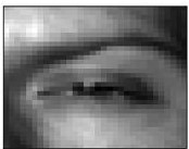
(c) Right eye.

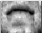
(d) Mouth.

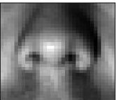
(e) Nose.

Figure 3: Sample images from the Augmented Extended Yale-B Dataset.

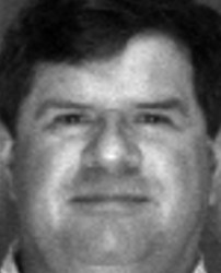
(a) Visible.

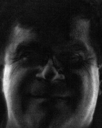
(b) DoLP.

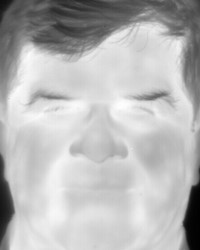
(c) S0.

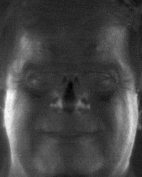
(d) S1.

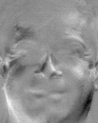
(e) S2.

Figure 4: Sample images from the ARL Polarimetric Dataset.

4.2 Network Structure

In the following, we will elaborate on how we construct the neural network for each dataset. Similarly to Abavisani and Patel (2018), we implemented DRoGSuRe with Tensorflow and used the adaptive momentum based gradient descent method (ADAM) Kingma and Ba (2014) to minimize the loss function in Equation (5) with a learning rate of $10^{-3}$.

4.2.1 ARL Dataset

In case of ARL dataset, we have five data modalities and will therefore have 5 different encoders, self expressive layers and decoders. Each encoder is composed of three neural layers. The first layer consists of 5 convolutional filters of kernel size 3. The second layer has 7 filters of kernel size 1. The last layer has 15 filters with kernel size equals 1.

4.2.2 EYB Dataset

For EYB dataset, we also have five data modalities, therefore, we have 5 different encoders, self expressive layers and decoders. Each encoder is composed of three neural layers. The first layer consists of 10 convolutional filters of kernel size 5. The second layer has 20 filters of kernel size 3. The last layer has 30 filters of kernel size 3.

4.3 Noiseless results

In the following, we compare the performance of our approach versus the DMSC approach when learning the union of subspaces structure of noise-free data. First, we divide each dataset into training and validation sets to be able to classify a newly observed dataset, using the structure learned through the current unlabeled data. The ARL expression dataset used for training consists of 2160 images per modality. The validation baseline images include 720 images total per modality. For the EYB, we randomly selected 1520 images per modality for training and 904 images for validation.The sparse solution $\mathbf{W}(t)$ corresponding to each data modality, provides important information about the relations among data points, which may be used to split data into individual clusters residing in a common subspace. Observations from each object can be seen as data points spanning one subspace. Interpreting the subspace-based affinities based on $\mathbf{W}(t)$ as a layered set of networks, we proceed to carry out what amounts to modality fusion. The $T$ sparse matrices are added to produce one sparse matrix for both modalities, $\mathbf{W}_{Total}$, thereby improving performance. Observations associated with one object individual are clustered as one subspace where the contribution of each sensor is embedded in the entries of the $\mathbf{W}_{Total}$ matrix. For clustering by $\mathbf{W}_{Total}$, we apply spectral clustering.

After learning the structure of the data clusters, we validate our results on the validation set. We extract the principal components (eigen vectors of the covariance matrix) of each cluster in the original (training) dataset, to act as a representative subspace of its corresponding class. We subsequently project each new test point onto the subspace corresponding to each cluster, spanned by its principal components. The $l_{2}$ norm of the projection is then computed, and the class with the largest norm is selected to be the class of this test point. For DRoGSuRe, we use the coefficient matrix $\mathbf{W}_{total}$ in Equation (13) to cluster the test data points coming from all data modalities. We compare the clustering output labels with the ground truth for each dataset. The results for ARL and EYB datasets are depicted in Tables (1) and (2) respectively. From the results, it is clear that DRoGSuRE technique for the fused data remarkably outperforms DMSC in case of ARL dataset. However, in case of EYB dataset and in the noiseless case, DMSC performed better than DRoGSuRe.

Table 1: ARL dataset

	Learning	Validation
DMSC	97.59%	98.33%
DRoGSuRe	100%	100%

Table 2: EYB dataset

	Learning	Validation
DMSC	98.82%	98.89%
DRoGSuRe	98.42%	98.76%

4.4 Noise training with single and multiple modalities

In the following, we test the robustness of our approach in the case of noisy learning. We distort one modality at a time by shuffling the pixels of all images in that particular modality during the training phase. By doing so, we are perturbing the structure of the sparse coefficient matrix associated with that modality, thus impacting the overall W matrix for both DRoGSuRe and DMSC. Testing with clean data, i.e. no distortion, demonstrates the impact of perturbing the training and hence performing an inadequate training, e.g., insufficient data or non-convergence. This can also be considered as augmenting the training data with new information or a new view for one modality which might not necessarily contained in the testing or the validation data. Moreover, we repeat the same experiment with the distortion of two modalities before learning the sparse coefficient matrices for both DMSC and DRoGSuRe. The results for the ARL dataset are depicted in Table (3) and (4), while results for the EYB dataset are shown in Table (5) and (6). For ARL dataset, we refer to Visible, S0, S1, S2 and DoLP as Mod 0, 1, 2, 3 and 4 respectively. For EYB Dataset, we refer to Face, left eye, nose, mouth and right eye as mod 0, 1, 2, 3, and 4. We refer to each modality as Mod, where L denotes learning and V denotes validation results. From the results, it is clear that DRoGSuRe is showing a significant improvement in the clustering accuracy as compared to DMSC for both learning and validation set. The reason for that, is again, due to the fact that perturbing one or two modalities would have less impact on the overall performance for DRoGSuRe in comparison to DMSC.

Table 3: ARL data :Distorting One Modality

	DMSC L	DMSC V	DRoGSuRe L	DRoGSuRe V
Mod 0	87.17%	86.67 %	95.37%	95%
Mod 1	91.67%	90%	98.29%	98.33%
Mod 2	92.77%	92.78%	99.17%	99.44%
Mod 3	90.55%	90.57%	99.31%	99.44%
Mod 4	92.78%	91.11%	96.44%	96.67%

Table 4: ARL data :Distorting Two Modalities

	DMSC L	DMSC V	DRoGSuRe L	DRoGSuRe V
Mod 0 & 1	82.22%	82.78%	92.27%	94.58%
Mod 1 & 2	91.11%	91.11%	97.22%	97.36%
Mod 0 & 3	85.51%	82.56%	93.01%	95.42%
Mod 1 & 4	91.67%	89.44%	97.22%	97.36%
Mod 2 & 3	90%	89.72%	97.69%	97.78%

Table 5: EYB data :Distorting One Modality

	DMSC L	DMSC V	DRoGSuRe L	DRoGSuRe V
Mod 0	87.96%	88.5%	93.29%	94.69%
Mod 1	91.84%	91.15%	95.79%	97.46%
Mod 2	89.01%	88.72%	98.03%	97.57%
Mod 3	92.69%	91.81%	95.59%	96.68%
Mod 4	91.45%	91.59%	97.17%	97.35%

Table 6: EYB data :Distorting Two Modalities

	DMSC L	DMSC V	DRoGSuRe L	DRoGSuRe V
Mod 0 & 2	86.64%	85.18%	96.84%	96.13%
Mod 0 & 4	87.83%	89.16%	94.54%	95.8%
Mod 1 & 4	86.38%	86.06%	94.21%	95.8%
Mod 2 & 3	88.22%	84.96%	91.58%	93.92%
Mod 3 & 4	88.03%	86.28%	94.08%	95.35%

4.5 Testing with limited noisy testing data

In the following, we study the effect of using noiseless data for training while validating with noisy and missing data. We add Gaussian noise to one data modality in the validation set, and vary the SNR by varying the noise variance. We subsequently assume that we only have one modality available at testing. Then, we keep increasing the number of available noiseless data modalities beside the noisy modality. We average the results considering all different combinations of data modalities for ARL and EYB datasets. The results are depicted in Figure (5) and (6) respectively. For the ARL dataset, we note the increasing gap between DMSC and DRoGSuRe as we augment the sensing capacity with noise-free modalities. On the other hand, for the EYB dataset and at lower SNR, the performance of DRoGSuRe is slightly worse than DMSC which might be explained by the results in Table II; as the training accuracy for DMSC is slightly better than DRoGSuRe in the case of clean training. However, at higher SNR, the performance of the two approaches is very close.

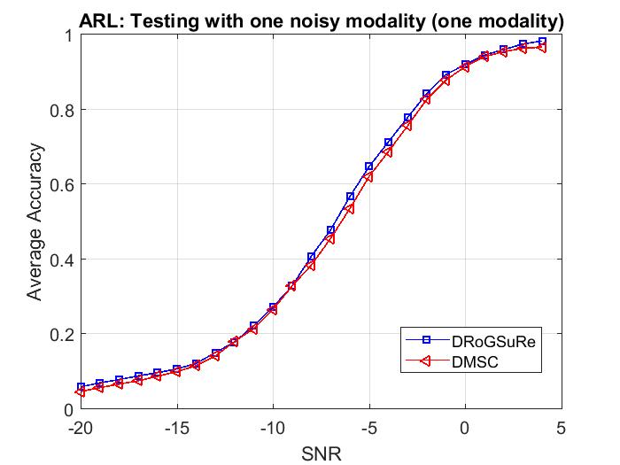
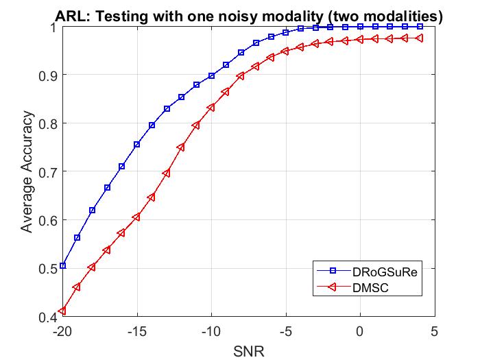
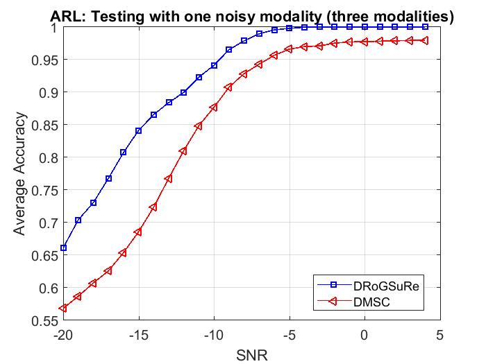
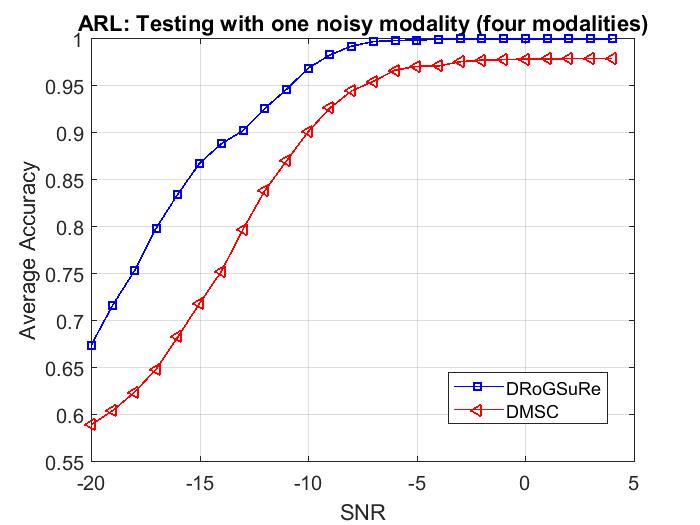
Figure 5: ARL Noiseless Training and validating on limited noisy data.

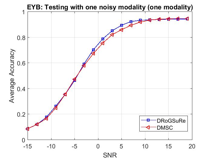
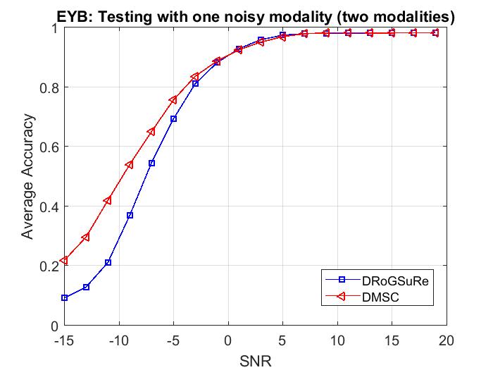
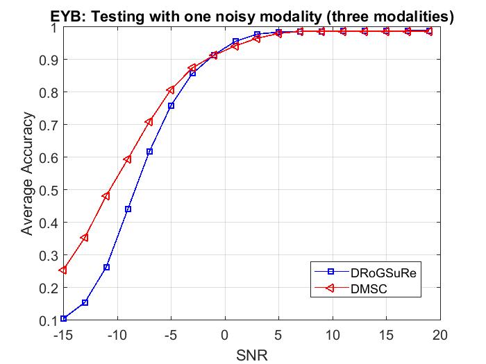
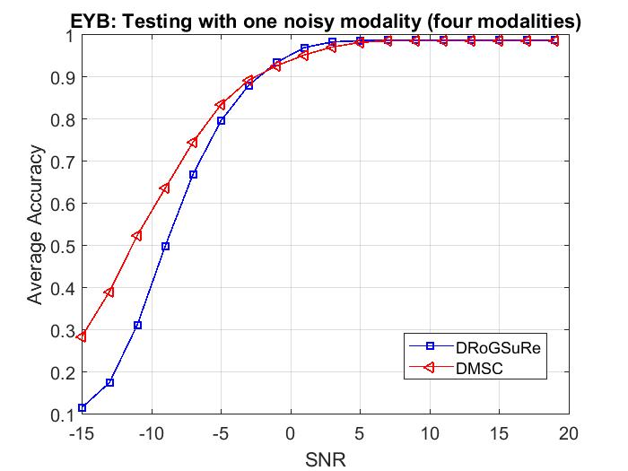
Figure 6: EYB Noiseless Training and validating on limited noisy data.

4.6 Missing modalities during testing

In the following, we evaluate the performance of DRoGSuRe and DMSC in case of missing data modalities during testing. It is not uncommon to have one or more sensors that might be silent during testing, thus justifying this experiment for further assessment. We try different combinations of available modalities during testing, and we average the clustering accuracy for each trial. Results are depicted in Figures (7) and (8) for ARL and EYB data respectively. Again, we notice a significant improvement for DRoGSuRe over DMSC for ARL Dataset. For EYB dataset, there is a slight improvement for DRoGSuRe over DMSC, however, the performance of DRoGSuRe is gracefully degrading while more modalities become unavailable during testing, which emphasizes the reliability and robustness of our proposed approach.

Figure 7: Missing modalities during testing for ARL dataset.

Figure 8: Missing modalities during testing for EYB dataset.

5 Feature Concatenation

Here we propose a rationale along with an alternative solution for enhancing the performance for EYB multi-modal data. Due to the specific structure of the EYB multi-modal data, the concatenation of the features corresponding to each modality is a reasonable alternative. By doing so, we are adjoining together the features representing each part of the face. Since the four modalities correspond to non-overlapping partitions of the face, the feature set corresponding to each partition will solely provide complementing information. A similar idea is proposed in Abavisani and Patel (2018) and is referred to as Late concatenation, where the multi-modal data is integrated in the last stage of the encoder. Their resulting decoder structure remains the same for either affinity fusion or late concatenation. This entails deconcatenating the multi-modal data prior to decoding it. Our proposed approach on the other hand, results in a self-expressive layer being driven by the concatenated features from the $M$ encoder branches. Afterwards, we feed the self-expressive layer output to each branch of the decoder. The concatenated information results in a more efficient code for the data, thereby resulting in an overall parsimonious with a sparse structure of the decoder, results in a decoder composed of three neural layers. The first layer consists of 150 filters of kernel size 3. The second layer consists of 20 layers of kernel size 3. The third layer consists of 10 layers of kernel size 5. Our approach is illustrated in Figure (9). We optimize the weights of the auto-encoder as follows,

$$\begin{split}\min\limits_{\mathbf{W}\mid w_{kk}=0}\rho\parallel\mathbf{W}\parallel_{1}+\frac{\gamma}{2}\sum_{t=1}^{T}\parallel X(t)-X_{r}(t)\parallel_{F}^{2}+\frac{\mu}{2}\parallel N-NW\parallel_{F}^{2}.\end{split}$$ (18)

where $N=[L(1)||L(2)||L(3)||L(4)||L(5)]$

Figure 9: CNN Concatenation Network

.

We compared the performance of our proposed approach against the late concatenation approach in Abavisani and Patel (2018) and the results are depicted in Table 7 for the EYB dataset.

Table 7: EYB dataset

	Learning	Validation
DMSC Late Concatenation	95.66%	94.7%
CNN Concatenation Network	99.28%	99.3%

From the previous table, we can conclude that concatenating the features from the encoder and feeding the concatenated information to each decoder branch achieves a better performance for this type of multi-modal data structure. The reason behind this enhancement is the combination of efficient extraction of the basic features from the whole face and finer features from each part of the face. Promoting more efficiency as noted, this concatenation may also be intuitively viewed as adequate mosaicking, in which different patterns complement each other. In the following, we will show how our proposed approach performs in two cases; missing and noisy test data. The results of the new proposed approach, which we refer to as CNN concatenation network, is compared to the state-of-the-art DMSC network Abavisani and Patel (2018). We start by training the auto-encoder network using 75% of the data and then we test on the rest of the data. In Figure 10, we show how the performance degrades by decreasing the number of available modalities at testing from five to one. From the results, it is clear how the CNN concatenation network outperforms the DMSC network. Additionally, we repeated the same experiment we performed in subsection 4.5. We train the network with noiseless data and then add Gaussian noise to one data modality at the testing. Additionally, we vary the number of available modalities at testing from one to four. The results are depicted in Figure 11. From the results, it is clear how the concatenated CNN network is more robust to noise than DMSC.

Figure 10: Missing modalities during testing

.

Figure 11: EYB Noiseless Training and validating on limited noisy data.

In addition, we have utilized the Concatenation network to perform object clustering on the ARL data. We compare the clustering performance of the concatenation network with both DMSC and DRoGSuRe. The results are depicted in Table 8. From the results, we conclude that DRoGSuRe still outperforms the other approaches for the ARL dataset. Although the number of parameters involved in training the DRoGSuRe network is higher than other approaches, since there are multiple self expressive layers, however, DRoGSuRe is more robust to noise and limited data availability during testing.

Table 8: ARL dataset

	Learning	Validation
DMSC	97.59%	98.33%
DRoGSuRe	100%	100%
CNN Concat	99.44%	99.17%

5.1 Deeper Network

In this work, we addressed the multi-modal data fusion by building on Deep Subspace Clustering, and we compare our approach to deep multimodal subspace clustering network Abavisani and Patel (2018) which in some sense dictated our following the same network structure in their paper so that we can have a fair comparison with their approach. In this section, we will consider a deeper alternative for the concatenation network and evaluate its performance. In Tables 7 and 8, we showed the results for the 3-layered concatenation network using ARL and EYB, respectively. Both the encoder and the decoder had three layers. We considered using 4, 5, and 6 layers in the auto-encoder for both the ARL and EYB to test deeper networks. The results are listed in Table 9. From the results, it is clear that adding more layers to the network does not improve the classification accuracy, which we believe is due to the dimensionality of the images in both datasets. All images are 32 $\times$ 32, and might not need additional layers to capture the image details.

Table 9: Deep Network

	4 layers			5 layers			6 layers
	ACC	ARI	NMI	ACC	ARI	NMI	ACC	ARI	NMI
ARL	99.4%	99.67%	98.94%	99.31%	99.6%	98.76%	99.26%	99.55%	98.66%
EYB	99.14%	98.9%	98.23%	97.43%	97.13%	94.77%	63.88%	58.31%	68.83%

6 Conclusion

In this paper, we proposed a deep multi-modal approach to fuse data through recovering the underlying subspaces of data observations from data corrupted by noise to scale to complex data scenarios. DRoGSuRe provides a natural way to fuse multi-modal data by employing the self representation matrix as an embedding for each data modality. Experimental results show a significant improvement for DRoGSuRe over DMSC under different types of potential limitations and provides robustness with limited sensing modalities. We also proposed the concatenated CNN network model, which can work better for different multi-modal data structures.

Appendix A Parameter Perturbation Analysis

To theoretically compare our proposed variational scaling fusion approach DRoGSuRe to DMSC, we proceed by way of a first order perturbation analysis on the parameter set $W^{i}$of respectively either technique $i=$1,2. This will, in turn impact the associated affinity matrix $A^{i}$, which as we will later elaborate directly impacts the subspace clustering procedure which is central to the inference following the fusion procedure.

Adopting the original formulation for the first persistently differential scaling approach, namely that T modalities are jointly exploited, results in, $X^{1}(t)=[x_{1}^{1}(t)x_{2}^{1}(t)...x_{n}^{1}(t)]$, where $x_{k}^{1}(t)\in\mathbb{R}^{m},t=1,2,...,T$ represents the $k^{th}$ observation. The second approach only effectively uses only one subspace structure of the fused modalities$X^{2}(t)=[x_{1}^{2}x_{2}^{2}...x_{n}^{2}]$. A first order perturbation on the data may be due to noise or to a degradation of a given sensor, and results in a perturbation of the UoS parameters,

$$\tilde{W}^{i}_{1}=W^{i}_{1}+\delta^{i}$$ (19)

For the first method, each modality will have an associated subspace cluster parameter set $\{W_{t}^{1}\}_{t=1,...,T}$, with $W_{t}^{1}\in\mathbb{R}^{n\times n}$. The overall parameter set for DRoGSuRe can then be written as,

$$\tilde{W}^{1}=\tilde{W}^{1}_{1}+W^{1}_{2}+...+W_{m}^{1}$$ (20)

Where the unperturbed overall sparse coefficient matrix is written as follows, $W_{tot}^{1}=W_{1}^{1}+W_{2}^{1}+...+W_{m}^{1}$. A similar development follows for method 2, with the difference that the contributing modalities are fused a priori.

Proof

We first write the affinity matrix associated with DRoGSuRE as,

$$\tilde{A}^{1}=\tilde{W}^{1}_{tot}+(\tilde{W}^{1}_{tot})^{T}$$ (21)

$$\tilde{A}^{1}=\tilde{W}^{1}_{1}+W^{1}_{2}+...+W_{m}^{1}+(\tilde{W}^{1}_{1}+W^{1}_{2}+...+W_{m}^{1})^{T}$$ (22)

Where the superscript $T$ denotes transpose. This is equivalent to,

$$\tilde{A}^{1}=\tilde{A}^{1}_{1}+\sum_{i=2}^{T}A_{i}^{1},$$ (23)

Where $0\leq\tilde{A}_{1}^{1}(i,j)\leq 1+\delta^{1}$. The unperturbed collective affinity matrix $A^{1}$ can be similarly written $A^{1}=\sum_{i=1}^{T}A_{i}^{1}$ with the unity constraint on each entry of all matrices. We may also write the magnitude of the difference as,

$$\lvert A^{1}-\tilde{A}^{1}\rvert=\delta^{1}+(\delta^{1})^{T}$$ (24)

Letting $\Delta=\delta^{1}+(\delta^{1})^{T}\in\mathbb{R}^{n\times n}$, i.e., $\Delta\in\mathbb{R}^{n\times n}$ and assuming $\epsilon=\max_{i,j}[\Delta]_{i,j}$, we can write,

$$\parallel A-\tilde{A}\parallel_{F}\leq n\epsilon$$ (25)

Given the $\Delta$ matrix individual entry bounds , we conclude that,

$$0\leq\epsilon\leq\frac{1}{t}$$ (26)

Since DMSC assumes having one sparse coefficient matrix W for all data modalities , which is equivalent to only one subspace structure of the fused modalities $X^{2}(t)=[x^{2}_{1}...x_{n}^{2}]$. Therefore, the UoS parameters will be perturbed by $\delta^{2}$ as follows,

$$\tilde{W}^{2}=W^{2}+\delta^{2}$$ (27)

The affinity matrix associated with DMSC can be written as follows, $\tilde{A}^{2}=\tilde{W}^{2}+(\tilde{W}^{2})^{T}$, which is equivalent to,

$$\tilde{A}^{2}=W^{2}+\delta^{2}+(W^{2})^{T}+(\delta^{2})^{T}$$ (28)

Similarly, the unperturbed affinity matrix will be as follows,

$$A^{2}=W^{2}+(W^{2})^{T}$$ (29)

From Eqns. 28 and 29, the magnitude of the difference can be written as follows,

$$\lvert A^{2}-\tilde{A}^{2}\rvert=\delta^{2}+(\delta^{2})^{T}$$ (30)

Letting $\gamma=\delta^{2}+(\delta^{2})^{T}\in\mathbb{R}^{n\times n}$, i.e., $\lvert A^{2}-\tilde{A}^{2}\rvert=\gamma$, and assuming $\psi=\max_{i,j}[\gamma]_{ij}$, we can write $\parallel A^{2}-\tilde{A}^{2}\parallel_{F}\leq n\psi$ . Given the $\gamma$ matrix individual entry bounds, we conclude $0\leq\psi\leq 1$. If we only perturb one modality, knowing that $0\leq A(i,j)\leq 1$, therefore the error could lie between $0\leq\psi\leq 1$, which entails either creating a fake relation between two data points or erasing an existing relation. $\epsilon$ and $\psi$ are random variables that do not have to follow a specific distribution, however, in any case $E(\epsilon^{2})\ll E(\psi^{2})$and therefore $SNR_{DRoGSuRe}\gg SNR_{DMSC}$

In light of the above two bounds, and the results of Hunter and Strohmer (2010), where it is shown that the spectral clustering dependent on the respective projection operators $P_{W^{1}}$ and $\tilde{P}_{\tilde{W}^{1}}$ onto the vector subspaces spanned by the principal eigenvectors of $W^{1}_{tot}$ and $\tilde{W}^{1}_{tot}$ of may be written as,

$$\parallel P_{W^{1}}-\tilde{P}_{\tilde{W}^{1}}\parallel_{F}\leq\frac{\sqrt{2}}{\alpha^{1}}\parallel A^{1}-\tilde{A}^{1}\parallel_{F},$$ (31)

where $\alpha^{1}$ is the spectral gap between the $k^{th}$ and $k+1^{st}$ eigen value of $A^{1}$, $\lvert\lambda^{1}_{k}-\lambda^{1}_{k+1}\rvert$. Similarly, for DMSC, the bound on the projection operators is,

$$\parallel P_{W^{2}}-\tilde{P}_{\tilde{W}^{2}}\parallel_{F}\leq\frac{\sqrt{2}}{\alpha^{2}}\parallel A^{2}-\tilde{A}^{2}\parallel_{F},$$ (32)

where $\alpha^{2}=\lvert\lambda^{1}_{k}-\lambda^{1}_{k+1}\rvert$. Since $W_{1}^{1},W_{2}^{1},...,W_{T}^{1}$ happen to commute and if they happen to be diagonalizable, therefore, they share the same eigenvectors. As a result, the eigenvectors of $W_{1}^{1}+W_{2}^{1}+...+W_{m}^{1}$ are also the same and the corresponding eigenvalue that is the sum of the corresponding eigenvalues of $W_{1}^{1},W_{2}^{1},..$ and $W_{T}^{1}$. As a result, we conclude that $\lambda_{k}^{2}$ Therefore, $\lambda_{k}^{1}\gg\lambda_{k}^{2}$. From all the above, we can conclude that smaller error yielding to better clustering, hence preserving the performance, yields the improvement by the T-factor noted in the proposition and shown in the two perturbation developments.

$\bf{Sally\ Ghanem}$ received the B.Sc. degree in electrical engineering from Alexandria University, in 2013, and the M.Sc. degree in electrical and computer engineering from North Carolina State University, Raleigh, NC, USA in 2016, where she is currently pursuing the Ph.D. degree. During the PhD program, she has spent time at Oak Ridge National Laboratory working on multimodal data. Her research interests include the areas of computer vision, digital signal processing, image processing and machine learning.

$\bf{Hamid\ Krim}$ received the B.Sc. and M.Sc. and Ph.D. in ECE. He was a Member of Technical Staff at AT&T Bell Labs, where he has conducted research and development in the areas of telephony and digital communication systems/subsystems. Following an NSF Postdoctoral Fellowship at Foreign Centers of Excellence, LSS/University of Orsay, Paris, France, he joined the Laboratory for Information and Decision Systems, MIT, Cambridge, MA, USA, as a Research Scientist and where he performed/supervised research. He is currently a Professor of electrical engineering in the Department of Electrical and Computer Engineering, North Carolina State University, NC, leading the Vision, Information, and Statistical Signal Theories and Applications Group. His research interests include statistical signal and image analysis and mathematical modeling with a keen emphasis on applied problems in classification and recognition using geometric and topological tools. He has served on the SP society Editorial Board and on TCs, and is the SP Distinguished Lecturer for 2015-2016.

References

- Abavisani and Patel (2018) Abavisani, M., Patel, V.M., 2018. Deep multimodal subspace clustering networks. IEEE Journal of Selected Topics in Signal Processing 12, 1601–1614.
- Bian and Krim (2015) Bian, X., Krim, H., 2015. Bi-sparsity pursuit for robust subspace recovery, in: 2015 IEEE International Conference on Image Processing (ICIP), IEEE. pp. 3535–3539.
- Bian et al. (2018) Bian, X., Panahi, A., Krim, H., 2018. Bi-sparsity pursuit: A paradigm for robust subspace recovery. Signal Processing 152, 148–159.
- Chen and Hero (2017) Chen, P.Y., Hero, A.O., 2017. Multilayer spectral graph clustering via convex layer aggregation: Theory and algorithms. IEEE Transactions on Signal and Information Processing over Networks 3, 553–567.
- Dong et al. (2013) Dong, X., Frossard, P., Vandergheynst, P., Nefedov, N., 2013. Clustering on multi-layer graphs via subspace analysis on grassmann manifolds. IEEE Transactions on signal processing 62, 905–918.
- Elhamifar and Vidal (2013) Elhamifar, E., Vidal, R., 2013. Sparse subspace clustering: Algorithm, theory, and applications. IEEE transactions on pattern analysis and machine intelligence 35, 2765–2781.
- Favaro et al. (2011) Favaro, P., Vidal, R., Ravichandran, A., 2011. A closed form solution to robust subspace estimation and clustering, in: CVPR 2011, IEEE. pp. 1801–1807.
- Gabriel et al. (2010) Gabriel, H.H., Spiliopoulou, M., Nanopoulos, A., 2010. Eigenvector-based clustering using aggregated similarity matrices, in: Proceedings of the 2010 ACM Symposium on Applied Computing, pp. 1083–1087.
- Ghanem et al. (2020) Ghanem, S., Panahi, A., Krim, H., Kerekes, R.A., 2020. Robust group subspace recovery: A new approach for multi-modality data fusion. IEEE Sensors Journal .
- Ghanem et al. (2018) Ghanem, S., Panahi, A., Krim, H., Kerekes, R.A., Mattingly, J., 2018. Information subspace-based fusion for vehicle classification, in: 2018 26th European Signal Processing Conference (EUSIPCO), IEEE. pp. 1612–1616.
- Ghanem et al. (2021) Ghanem, S., Roheda, S., Krim, H., 2021. Latent code-based fusion: A volterra neural network approach. arXiv preprint arXiv:2104.04829 .
- Hellwich and Wiedemann (2000) Hellwich, O., Wiedemann, C., 2000. Object extraction from high-resolution multisensor image data, in: Third International Conference Fusion of Earth Data, Sophia Antipolis.
- Ho et al. (2003) Ho, J., Yang, M.H., Lim, J., Lee, K.C., Kriegman, D., 2003. Clustering appearances of objects under varying illumination conditions, in: 2003 IEEE Computer Society Conference on Computer Vision and Pattern Recognition, 2003. Proceedings., IEEE. pp. I–I.
- Hong et al. (2006) Hong, W., Wright, J., Huang, K., Ma, Y., 2006. Multiscale hybrid linear models for lossy image representation. IEEE Transactions on Image Processing 15, 3655–3671.
- Hu et al. (2016) Hu, S., Short, N.J., Riggan, B.S., Gordon, C., Gurton, K.P., Thielke, M., Gurram, P., Chan, A.L., 2016. A polarimetric thermal database for face recognition research, in: Proceedings of the IEEE conference on computer vision and pattern recognition workshops, pp. 187–194.
- Hunter and Strohmer (2010) Hunter, B., Strohmer, T., 2010. Performance analysis of spectral clustering on compressed, incomplete and inaccurate measurements. arXiv preprint arXiv:1011.0997 .
- Ji et al. (2017) Ji, P., Zhang, T., Li, H., Salzmann, M., Reid, I., 2017. Deep subspace clustering networks, in: Advances in Neural Information Processing Systems, pp. 24–33.
- Kingma and Ba (2014) Kingma, D.P., Ba, J., 2014. Adam: A method for stochastic optimization. arXiv preprint arXiv:1412.6980 .
- Korona and Kokar (1996) Korona, Z., Kokar, M.M., 1996. Model theory based fusion framework with application to multisensor target recognition, in: 1996 IEEE/SICE/RSJ International Conference on Multisensor Fusion and Integration for Intelligent Systems (Cat. No. 96TH8242), IEEE. pp. 9–16.
- Lee et al. (2005) Lee, K.C., Ho, J., Kriegman, D.J., 2005. Acquiring linear subspaces for face recognition under variable lighting. IEEE Transactions on pattern analysis and machine intelligence 27, 684–698.
- Li and Vidal (2015) Li, C.G., Vidal, R., 2015. Structured sparse subspace clustering: A unified optimization framework, in: Proceedings of the IEEE conference on computer vision and pattern recognition, pp. 277–286.
- Lin et al. (2011) Lin, Z., Liu, R., Su, Z., 2011. Linearized alternating direction method with adaptive penalty for low-rank representation, in: Advances in neural information processing systems, pp. 612–620.
- Liu et al. (2012) Liu, G., Lin, Z., Yan, S., Sun, J., Yu, Y., Ma, Y., 2012. Robust recovery of subspace structures by low-rank representation. IEEE transactions on pattern analysis and machine intelligence 35, 171–184.
- Luenberger et al. (1984) Luenberger, D.G., Ye, Y., et al., 1984. Linear and nonlinear programming. volume 2. Springer.
- Ng et al. (2002) Ng, A.Y., Jordan, M.I., Weiss, Y., 2002. On spectral clustering: Analysis and an algorithm, in: Advances in neural information processing systems, pp. 849–856.
- Ngiam et al. (2011) Ngiam, J., Khosla, A., Kim, M., Nam, J., Lee, H., Ng, A., 2011. Multimodal deep learning (pp. 689–696), in: International conference on machine learning (ICML), Bellevue, WA.
- Ramachandram and Taylor (2017) Ramachandram, D., Taylor, G.W., 2017. Deep multimodal learning: A survey on recent advances and trends. IEEE Signal Processing Magazine 34, 96–108.
- Rockafellar (1974) Rockafellar, R.T., 1974. Augmented lagrange multiplier functions and duality in nonconvex programming. SIAM Journal on Control 12, 268–285.
- Roheda et al. (2018a) Roheda, S., Krim, H., Luo, Z.Q., Wu, T., 2018a. Decision level fusion: An event driven approach, in: 2018 26th European Signal Processing Conference (EUSIPCO), IEEE. pp. 2598–2602.
- Roheda et al. (2019) Roheda, S., Krim, H., Luo, Z.Q., Wu, T., 2019. Event driven fusion. arXiv preprint arXiv:1904.11520 .
- Roheda et al. (2020a) Roheda, S., Krim, H., Riggan, B.S., 2020a. Commuting conditional gans for multi-modal fusion, in: ICASSP 2020-2020 IEEE International Conference on Acoustics, Speech and Signal Processing (ICASSP), IEEE. pp. 3197–3201.
- Roheda et al. (2020b) Roheda, S., Krim, H., Riggan, B.S., 2020b. Robust multi-modal sensor fusion: An adversarial approach. IEEE Sensors Journal 21, 1885–1896.
- Roheda et al. (2018b) Roheda, S., Riggan, B.S., Krim, H., Dai, L., 2018b. Cross-modality distillation: A case for conditional generative adversarial networks, in: 2018 IEEE International Conference on Acoustics, Speech and Signal Processing (ICASSP), IEEE. pp. 2926–2930.
- Soong and Rosenberg (1988) Soong, F.K., Rosenberg, A.E., 1988. On the use of instantaneous and transitional spectral information in speaker recognition. IEEE Transactions on Acoustics, Speech, and Signal Processing 36, 871–879.
- Taylor et al. (2016) Taylor, D., Shai, S., Stanley, N., Mucha, P.J., 2016. Enhanced detectability of community structure in multilayer networks through layer aggregation. Physical review letters 116, 228301.
- Valada et al. (2016) Valada, A., Oliveira, G.L., Brox, T., Burgard, W., 2016. Deep multispectral semantic scene understanding of forested environments using multimodal fusion, in: International Symposium on Experimental Robotics, Springer. pp. 465–477.
- Wang et al. (2018) Wang, H., Skau, E., Krim, H., Cervone, G., 2018. Fusing heterogeneous data: A case for remote sensing and social media. IEEE Transactions on Geoscience and Remote Sensing 56, 6956–6968.
- Xu et al. (1992) Xu, L., Krzyzak, A., Suen, C.Y., 1992. Methods of combining multiple classifiers and their applications to handwriting recognition. IEEE transactions on systems, man, and cybernetics 22, 418–435.
- Yang et al. (2006) Yang, A.Y., Rao, S.R., Ma, Y., 2006. Robust statistical estimation and segmentation of multiple subspaces, in: 2006 Conference on Computer Vision and Pattern Recognition Workshop (CVPRW’06), IEEE. pp. 99–99.
- Zhu et al. (2019) Zhu, P., Hui, B., Zhang, C., Du, D., Wen, L., Hu, Q., 2019. Multi-view deep subspace clustering networks. arXiv preprint arXiv:1908.01978 .