Parallel Synthesis for Autoregressive Speech Generation

Abstract

Autoregressive models have achieved outstanding performance in neural speech synthesis tasks such as text-to-speech and voice conversion. A model with this autoregressive architecture predicts a sample at some time step conditioned on those at previous time steps. Though it can generate highly natural human speech, the iterative generation inevitably makes the synthesis time proportional to the utterance’s length, leading to low efficiency. Many works were dedicated to generating the whole speech time sequence in parallel and then proposed GAN-based, flow-based, and score-based models. This paper proposed a new thought for autoregressive generation. Instead of iteratively predicting samples in a time sequence, the proposed model performs frequency-wise autoregressive generation (FAR) and bit-wise autoregressive generation (BAR) to synthesize speech. In FAR, a speech utterance is first split into different frequency subbands. The proposed model generates a subband conditioned on the previously generated one. A full band speech can then be reconstructed by using these generated subbands and a synthesis filter bank. Similarly, in BAR, an 8-bit quantized signal is generated iteratively from the first bit. By redesigning the autoregressive method to compute in domains other than the time domain, the number of iterations in the proposed model is no longer proportional to the utterance’s length but the number of subbands/bits. The inference efficiency is hence significantly increased. Besides, a post-filter is employed to sample audio signals from output posteriors, and its training objective is designed based on the characteristics of the proposed autoregressive methods. The experimental results show that the proposed model is able to synthesize speech faster than real-time without GPU acceleration. Compared with the baseline autoregressive and non-autoregressive models, the proposed model achieves better MOS and shows its good generalization ability while synthesizing 44 kHz speech or utterances from unseen speakers.

I Introduction

Figure 1: Overview of different autoregressive methods and their orders of generation. (a) Conventional autoregressive generation. Samples at different time steps are generated sequentially. (b) Frequency-wise autoregressive generation (FAR). (c) Bit-wise autoregressive generation (BAR).

Neural speech synthesis has recently achieved remarkable audio qualities in different speech tasks such as text-to-speech (TTS) [1, 2, 3] and voice conversion (VC) [4]. These systems typically comprise two separate models: a synthesizer and a vocoder. A synthesizer is usually designed for some specific speech task and outputs acoustic features such as linear-scaled spectrograms, Mel-spectrograms, F0 frequencies, spectral envelopes, or aperiodicity information [5, 6, 7, 8]. A vocoder is designed to reconstruct audio waveforms from the acoustic features [3, 9, 10]. In the early era of neural speech synthesis, a hand-crafted vocoder [10, 11, 12] or the Griffin-Lim algorithm [13] was adopted to reconstruct speech waveforms [5, 14, 15, 16, 17]. However, speech signals have a high temporal resolution, and neither conventional vocoders nor heuristic methods can reconstruct high-quality natural speech, remaining modeling raw audio a challenging problem. In Tacotron 2 [6], a neural network [3] is used as the vocoder to generate speech conditioned on Mel-spectrograms and has shown the potential of neural vocoder for synthesizing natural human speech.

Neural vocoders, while proposed for the TTS system, are not limited to this usage. A neural vocoder can be used for a wide range of applications associated with speech synthesis, such as TTS, VC, speech bandwidth extension (SBE), and speech compression (SC) [5, 2, 18, 4, 19, 20, 21, 22]. With high-quality vocoders involved, these models can focus only on processing acoustic features for different speech tasks instead of directly manipulating speech waveforms. As more and more models process and output acoustic features while using another neural network to reconstruct speech, the research about using neural vocoders for waveform modeling becomes influential on the naturalness of generated speech [23, 24, 25].

WaveNet, one of the earliest neural vocoders, adopted an autoregressive model to generate raw waveforms [3]. The model is conditioned on previously generated samples to predict that of the next time step. It is capable of generating high-quality speech and music samples. However, due to the properties of the autoregressive method, these models are inevitably slow and inefficient while iteratively predict audio samples, restricting the speech synthesis systems from real-time applications. Different variants of autoregressive vocoders [26, 9, 27] are proposed to increase efficiency, but the improvements are still limited.

To fix the low-speed generation issue of autoregressive models, significant efforts have been dedicated to the development of non-autoregressive models recently [28, 29, 30, 31, 32]. Non-Autoregressive models try to generate samples at different time steps in parallel. More specifically, the number of iterations in autoregressive methods is in proportion to the speech length, while non-autoregressive models generate a full-length utterance in one computation. While non-autoregressive models are faster at inference time, they often perform not as well as autoregressive models.

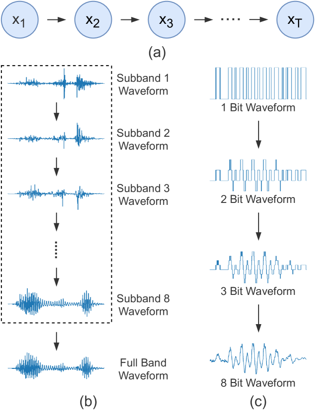
This paper aims to address the efficiency problem by exploring and redesigning the directions for autoregressive generation. Specifically, we propose to conduct autoregressive generation in domains other than the temporal one, and two new autoregressive methods are designed: frequency-wise autoregressive generation (FAR) and bit-wise autoregressive generation (BAR). In FAR, a full-band speech utterance is first divided into multiple frequency subbands by analysis filters. Autoregressively in the frequency domain, the model aims to learn to predict a subband signal given its previous subband. The model architecture is designed to generate a subband utterance in parallel, and the inference time of the proposed model is no longer proportional to the speech length but the number of subbands. Similar to FAR, in BAR, each speech sample is first quantized into an 8-bit representation using $\mu$-law companding transformation. The first bit, which represents the value is greater than or less than zero, is predicted first, and then the second and the third bits are predicted conditioned on the first and the second bits. Finally, the first three bits are used to generate a complete 8-bit signal sample.

Conventional autoregressive methods in the time domain generate samples conditioned on the information from the previous time step. These methods achieves better inference results. Similarly, the frequency-wise and bit-wise autoregressive methods can leverage the past and the future information from different subbands and bit precisions to make predictions, while the number of iterations is fixed regardless of the length of the speech. In addition to boosting the speech quality, the method for sampling from the output posteriors is also improved. Instead of randomly sampling, a post-filter is introduced to generate the final result from the posterior probability. The sampling method not only generates unquantized and high-fidelity signals but also leads to a more natural speech.

The contributions of this work are twofold. First, this paper is the first to explore and design new directions for autoregressive method to improve efficiency. Instead of in the time domain, the proposed model conduct autoregressive speech generation in the frequency domain and the bit precision domain. Second, a post-filter is applied to sample audio signals from output posteriors. We combine the characteristics of the proposed autoregressive methods to design the training objective for the post-filter. Both the objective and subjective experiment results show that the proposed new autoregressive model betters parallel synthesis methods in terms of speech quality and possesses comparable generated speech naturalness to autoregressive neural vocoders. While inference using a CPU or GPU, the synthesis speed achieves real-time and is as fast as parallel methods. In addition, the proposed autoregressive generation model can be applied not only on neural vocoder but on speech synthesis tasks such as voice conversion and text-to-speech to further improve the quality and efficiency.

This paper is organized as follows. In Section II, we first review previous vocoding methods including conventional, autoregressive, and non-autoregressive vocoders. In Section III, we described the proposed autoregressive framework, posterior sampling method, and vocoder architecture for the experiments. Section IV details the experimental setup , and Section V shows the results. The conclusion is given in Section VI.

II Related Work

A vocoder aims to synthesize a speech utterance with given acoustic features. Before the era of neural vocoder, parametric vocoders such as STRAIGHT [11] and WORLD [10] are usually designed according to signal processing techniques. The speech qualities of these methods are limited, and later neural vocoders are proposed and demonstrated the ability to synthesize natural speech.

In the beginning, most of the neural vocoders for speech synthesis are autoregressive, meaning that they condition future audio samples on previous samples to model long-term dependencies in speech waveform. WaveNet [3], as the most representative autoregressive neural vocoder, models the waveform using dilated convolutional layers and gated activation units from [33]. In WaveRNN [9], the model architecture is simplified by replacing the deep convolutional networks with recurrent neural networks. LPCNet [27] further adopts the linear prediction technique. These approaches are relatively simple to implement and train. However, they are inherently serial and hence can not fully utilize parallel processors like GPUs or TPUs. Therefore, autoregressive models have difficulty synthesizing audio in real-time.

Figure 2: (a) Conventional autoregressive model. Each blue circle represents a scalar. (b) Proposed autoregressive model. The speech is generated iteratively in the frequency domain or the bit precision domain. Each green block is the model illustrated in Fig. 5 (a), and each orange block represents a time series.

Recently, a bunch of non-autoregressive models has been proposed to fix the inference speed issue of the autoregressive method. Some works try to distill the output of the autoregressive model to a non-autoregressive model, for example, Parallel WaveNet [28] and Clarinet [29]. The student networks underlying both Parallel WaveNet and Clarinet are based on inverse autoregressive flow (IAF) [34]. Though the IAF network can run in parallel at inference time, the teacher-student-based knowledge distillation strategy makes the training process inefficient and the whole framework complicated.

Inspired by the success of the flow-based model in the image generation GLOW [35], WaveGlow [30] is proposed. Instead of the autoregressive process in IAF, WaveGlow adopts the affine coupling layer, which is more efficient, and the synthesis speed is 25 times faster than real-time. Another group of vocoders utilizes generative adversarial networks (GAN), which calculate the probability implicitly, for example, MelGAN [36] and Parallel WaveGAN [31]. Aside from the flow-based and GAN-base models, a score-based method, such as WaveGrad [32], models the multi-step generation as a Markov process, which can polish the speech quality over steps according to the time budget.

In this paper, we propose two new methods for autoregressive vocoders, FAR and BAR. Compared with conventional autoregressive models, the proposed model iteratively generates signals of different subbands or bit precisions and predicts samples at all time steps simultaneously. The autoregressive characteristic also makes the proposed model outperform the competitive non-autoregressive model in our experiments. We also employ a post-filter to sample audio signals from output posteriors and design a training objective based on the characteristics of the proposed methods, which have not been done before.

III Proposed Method

III-A Rethinking the Direction for Autoregressive generation

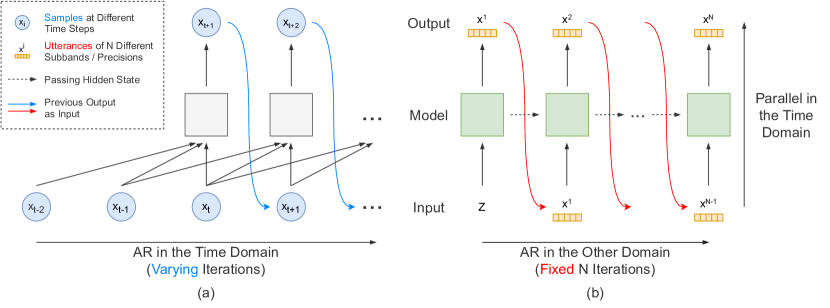
The conventional autoregressive neural vocoder, as shown in Fig. 2 (a), formulates the synthesis problem as maximizing the joint probability of a waveform $X=\{x_{1},x_{2},...,x_{T}\}$, which can be factorized as follows:

$$p(X)=\prod_{t=1}^{T}p(x_{t}|x_{1},x_{2},...,x_{t-1}),$$ (1)

where $x_{t}$ is the audio sample at time $t$ and generated conditioning on signals from previous timesteps. Teacher forcing can be easily applied for parallel computing during training. While at inference time, the signal $x_{t}$ at time $t$ is not able to be predicted until all $x_{1},x_{2},...,x_{t-1}$ are inferred. The total iterations and time are inevitably proportional to the target audio length. Twenty-two thousand calculations are conducted iteratively to generate a one-second speech with a 22 kHz sampling rate.

To increase the inference efficiency and preserve the quality, we redesign the autoregressive method to compute in domains other than the temporal one. A waveform sequence $X$ is first split into $N$ subsequences, $x^{1},x^{2},...,x^{N}$, where $N$ is some fixed number, and each $x^{n}$ is a time series. As shown in Fig. 2 (b), the prediction of the $n$th subsequence $x^{n}$ is conditioned on the previous subsequence $x^{n-1}$. Eq. 1 can be reformulated as follows:

$$p(X)=\prod_{n=1}^{N}p(x^{n}|x^{n-1}).$$ (2)

The redesigned process takes fixed $N$ iterations in total and can be parallel in the time domain by designing the model architecture, e.g., using only layers of CNN. We will discuss the splitting methods in Section III-B and III-C. Note that the conditioning acoustic features are omitted and will be detailed in Section III-D.

Figure 3: Frequency-wise autoregressive generation.

III-B Frequency-wise Autoregressive Generation (FAR)

The first splitting method is subband analysis, which divides a speech utterance into multiple subband signals using a subband analysis filter bank, and each represents information in different frequency bands. The analysis process can be written as follows:

$$\{x^{1},x^{2},...,x^{N}\}=\phi(X),$$ (3)

where $\phi$ is the analysis filter bank, $N$ is the number of subband, and $x^{i}$ is the $i$th subband utterance. While splitting a signal with length $L$ into $N$ subband signals, each length is shortened to $L/N$. Though some works leverage this method to improve the efficiency of autoregressive vocoders [37, 38, 39], they only make use of the property of length shortening to enable models to synthesize $N$ shorter subband utterances in parallel. The inference time still grows substantially as the signal length increases.

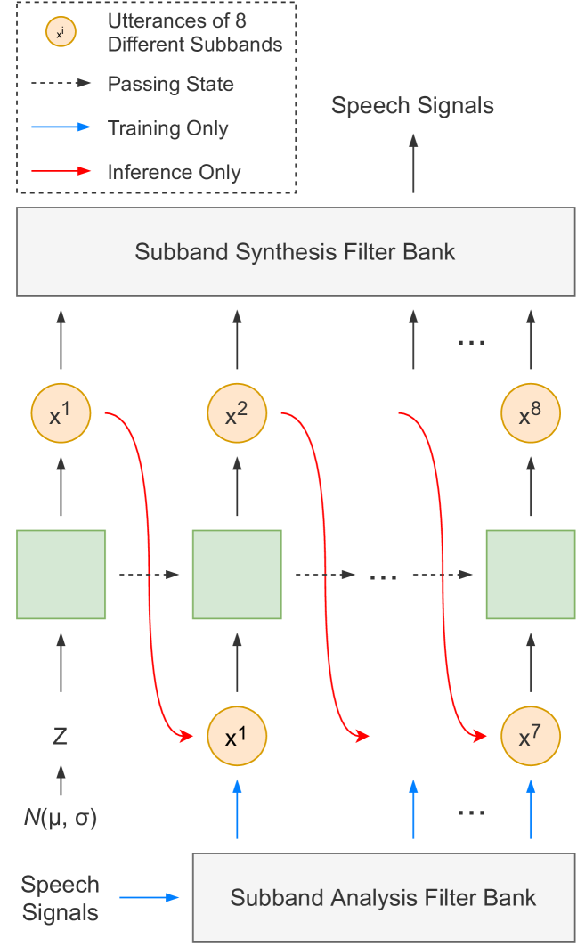
In FAR, we replace the time domain with the frequency domain for autoregressive generation, making the model compute parallelly in the time domain and instead perform autoregressive synthesis in the frequency domain. As shown in Fig. 3, the model first takes as input a noise $Z$ from the normal distribution $N(\mu,\sigma)$ and generates the signal of the first subband, $x^{1}$. In each forward operation, $x^{i}$ serves as a condition to generate the next subband signal, $x^{i+1}$. Finally, a full band L-length speech $X$ can be generated with N different subband signals and a synthesis filter bank $\psi$:

$$X=\psi(x^{1},x^{2},...,x^{N}).$$ (4)

We follow [40] to design analysis and synthesis filter banks. In our proposed model, a speech utterance is divided into eight subband signals, and the model iteratively generates from the subband with the highest frequency to the one with the lowest. The total number of iterations is consequently fixed to eight, which is much less than that in traditional autoregressive methods and makes the model more efficient.

Figure 4: Bit-wise autoregressive generation.

III-C Bit-wise Autoregressive Generation (BAR)

FAR enables models to generate speech samples with a fixed number of iterations while conditioned on the previous and future information. To provide more information for autoregressive speech generation, in this section, we further investigated another domain to split the signals. The proposed BAR is an autoregressive method in the bit precision domain.

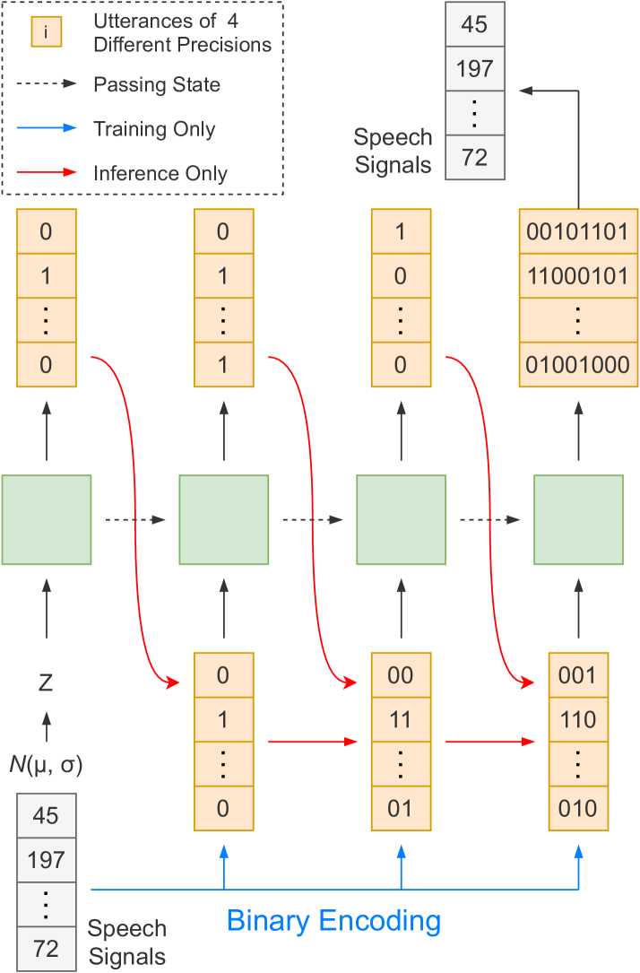
In BAR, we follow [3] to model the output as 8-bit samples transformed by $\mu$-law algorithm, and each sample is a binary sequence of length eight representing the value ranging from 0 to 255. As shown in Fig. 4, the first step is to take a randomly initialized vector $Z$ as input to generate the first bits (0 or 1) of the samples at different time steps. The first bit represents whether the value of this speech sample is greater than 127. All previous bits are used as conditions to generate the next bits. The output signals gradually become more precise as the bits are predicted. Though the model can iteratively generate all bits in the binary sequence, we empirically found that a complete 8-bit signal can be directly predicted conditioned only on the first three bits, making the total number of iterations fixed at four.

Figure 5: (a) Overview of the proposed model architecture. $x$ is the subband utterance, $f$ is the upsampled acoustic features, and $h$ is the hidden state. $b^{1},b^{2},b^{3}$ are the first, second, and third bit of $x$. (b) WN module.

III-D Proposed Vocoder Architecture

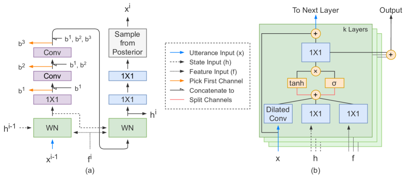
In the previous sections, we introduced a new concept for autoregressive generation and demonstrated two implementation methods. In this part, we detail how to combine FAR and BAR with an autoregressive neural vocoder. We modify the architecture from [3] for the following experiments. Note that FAR and BAR can be applied to vocoders with different architectures, such as GAN-based [31, 41], flow-based [30], and other models [3, 9, 27].

Fig. 5 (a) shows the overview of the model. The model consists of WN modules (WN), convolutional layers with kernel size 5 (Conv), and convolutional layers with kernel size 1 (1X1). Fig. 5 (b) shows the WN module. The module is mainly composed of dilated convolutional layers and gated activation units [33]. This architecture is proposed in WaveNet [3] and shows effectiveness for speech processing in many works [30, 31, 42, 43].

To conduct FAR, the model takes $x^{i-1}$ as input and output the ith subband utterance $x^{i}$. The acoustic features (e.g., Mel-spectrogram) are upsampled to the same length as the target, denoted as $f^{i}$ for the ith subband generation. Inspired by [9], we use $h^{i}$ as a hidden state to pass information across different iterations. We denote the model as $FAR$ and formulate the process as follows:

$$x^{i},h^{i}=FAR(x^{i-1},h^{i-1},f^{i}).$$ (5)

BAR is integrated into each FAR iteration, which is shown as purple blocks in Fig. 5 (a). The first channel of each convolutional layer output is used to predict the first three bits of the target sequence, denoted as $b^{1}$, $b^{2}$, and $b^{3}$. The remaining channels are passed to a Mish activation function [44] and be concatenated with predicted bits (ground-truth bits during training) as input of the next layer. The target utterance is then predicted using a WN module and two 1X1 layers followed by Mish activation layers.

Denote the output for predicting $b^{1}$, $b^{2}$, $b^{3}$, and $x^{i}$ as $p_{b^{1}}$, $p_{b^{2}}$, $p_{b^{3}}$, and $p_{x^{i}}$, the process of sampling from posterior is formulate as follows:

$$b^{1}=Sample(\sigma(10\times p_{b^{1}})),$$ (6)

$$b^{2}=Sample(\sigma(10\times p_{b^{2}})),$$ (7)

$$b^{3}=Sample(\sigma(5\times p_{b^{3}})),$$ (8)

$$x^{i}=Sample(Softmax(10\times p_{x^{i}})),$$ (9)

where $Sample$ is randomly sampling from probabilities and can be a post-filter network when predicting $x^{i}$, which will be detailed in the next section. Each posterior is multiplied by a scalar to make the distribution steeper and less noisy. We use the cross-entropy (CE) loss for training [3, 9, 27].

III-E Post-filtering for Posterior Sampling

Figure 6: Different methods to sample output from posteriorgram. Argmax: Choosing the category with the greatest probability. Sample: Sampling according to the probability distribution. Post-Filtering: Using a network to predict the 16-bit sample.

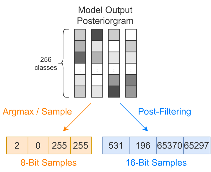
The output of a conventional autoregressive vocoder is usually a sequence of probability distributions [3, 9, 27], and waveform signals can be generated by two different methods: (1) Selecting the category with the most significant probability (Argmax). (2) Random sampling according to the probability distributions (Sample). The orange path in Fig. 6 represents these two sampling methods. In this section, instead of handcrafted sampling methods, we proposed to use a neural network as a post-filter for sampling (the blue path in Fig. 6). Post-filtering has shown effective in helping improving speech quality and convergence speed in [45]. The network is designed to learn how to sample and improve the detail and fidelity of signals (from 8-bit to 16-bit). Instead of a posterior distribution, the post-filter directly output the subband signals. The process is formulated as:

$$x^{i}=PF(AR(x^{i-1})),$$ (10)

where $PF$ is the post-filter, $AR$ is any autoregressive model mentioned above, and $x^{i}$ denotes the ith subsequence defined in Section III-A.

Figure 7: Two paths for post-filter training.

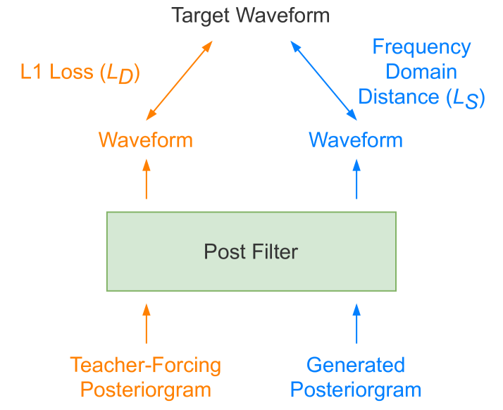
An autoregressive model is trained under teacher-forcing manners, which means $x^{i}$ is generated conditioned on its previous ground truth subsequence $\hat{x}^{i-1}$. Two different types of posteriorgram, $AR(\hat{x}^{i-1})$ and $AR(x^{i-1})$, can be used for trainig $PF$, formulated as follows:

$$x_{tf}^{i}=PF(AR(\hat{x}^{i-1})),$$ (11)

$$x_{ntf}^{i}=PF(AR(x_{ntf}^{i-1})).$$ (12)

Note that at inference time, $PF$ works the same as Eq. 12.

Fig. 7 shows the two training paths. We apply different loss functions as the input type changes. For Eq. 11 (the orange path), the loss $L_{D}$ is written as follows:

$$L_{D}=\frac{1}{N+1}(MAE(X_{tf},\hat{X})+\sum_{i=1}^{N}MAE(x_{tf}^{i},\hat{x}^{i})),$$ (13)

where $X_{tf}=\psi(x_{tf}^{1},x_{tf}^{2},...,x_{tf}^{N})$, $\hat{X}=\psi(\hat{x}^{1},\hat{x}^{2},...,\hat{x}^{N})$, and $MAE$ is the mean absolute error.

Figure 8: Average pooling in $L_{S}$. (a) STFT magnitude. (b) Band-limited STFT magnitude.

As for Eq. 12 (the blue path), $L_{S}$ is designed to measure the distance between $X_{ntf}$ and $\hat{X}$ in the frequency domain, where $X_{ntf}=\psi(x_{ntf}^{1},x_{ntf}^{2},...,x_{ntf}^{N})$. This kind of measurement have been shown effective [46, 47, 31, 45, 41]. We modify the multi-resolution Short-time Fourier transform (STFT) auxiliary loss in [31] as follows:

$$L_{S}=\frac{1}{M}\sum_{m=1}^{M}(L_{sc}^{m}(X_{ntf},\hat{X})+L_{mag}^{m}(X_{ntf},\hat{X})),$$ (14)

where $M$ is the number of different parameter sets of STFT; $L_{sc}$ and $L_{mag}$ are the spectral convergence loss and log STFT-magnitude loss from [48]:

$$L_{sc}(a,b)=\frac{\left\|\left|STFT(a)\right|-\left|STFT(b)\right|\right\|_{F}}{\left\|\left|STFT(a)\right|\right\|_{F}},$$ (15)

$$L_{mag}(a,b)=\frac{1}{N_{mag}}\left\|log\left|STFT(a)\right|-log\left|STFT(b)\right|\right\|_{1},$$ (16)

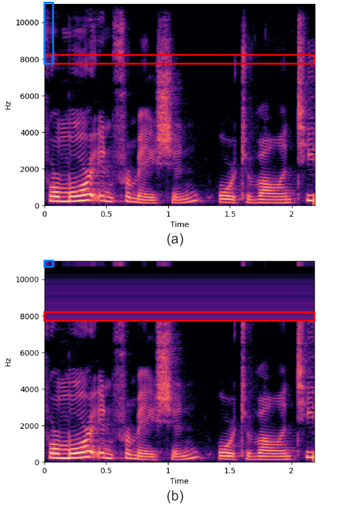
where $N_{mag}$ is the number of elements in the magnitude, $\left\|\cdot\right\|_{F}$ is the Frobenius norm, and $\left\|\cdot\right\|_{1}$ is the $L_{1}$ norm. $\left|STFT(\cdot)\right|$ is the band-limited STFT magnitude. We use the magnitude information with the frequency ranging from 0 to 8000 Hz. Magnitudes with higher frequency are average pooled in the frequency and time axes to extract only local and global energy information. As shown in Fig. 8 (a). The blue box represents calculating the average per frame; the red box represents calculating the average per frequency. Fig. 8 (b) is the extracted magnitude. The blue box represents an average per frame (duplicated along the frequency axis for visualization); the red box represents an average per frequency, and the value is duplicated along the time axis for calculating $L_{S}$. The average pooling is to reduce the synthetic noise resulting from applying $L_{S}$, as mentioned in [31, 45, 49]. The final loss function $L_{PF}$ is a linear combination of $L_{D}$ and $L_{S}$:

$$L_{PF}=100L_{D}+0.1L_{S}.$$ (17)

IV Experimental Setup

IV-A Dataset

Four datasets were used in our experiments.

• LJ Speech LJ Speech [50] is a high-quality speech dataset widely used for training and evaluating TTS models and neural vocoders. The audio clips are recorded with a sampling rate of 22 kHz by a female English speaker. It contains 13100 utterances, and the total duration is approximately 24 hours.

• VCTK CSTR’s VCTK corpus [51] is a multi-speaker English speech dataset containing about 44k utterances and transcriptions. Approximately 400 sentences were read by 109 English speakers with different accents. The total duration is about 44 hours. The audio clips are with a sampling rate of 48 kHz and downsampled to 22 kHz in our experiments.

• CMU ARCTIC Initially designed for unit selection speech synthesis, the CMU ARCTIC databases [52] consist of clean audio clips of different English speakers. We used utterances from a male (bdl) and a female (slt) speaker as a test set for experiments in Section V-C. All the utterances were downsampled to 22 kHz.

• Internal Mandarin Speech Corpus The corpus is designed for building Mandarin TTS systems. It consists of 9004 high-quality speech utterances of a Mandarin female speaker. The total duration is about 7 hours. We used the audio clips with a sampling rate of 44 kHz for high-fidelity speech synthesis.

IV-B Acoustic Feature

We used an 80-dimensional Mel-spectrogram as the conditioning acoustic feature for speech synthesis. For computing the STFT, the FFT size, hop size and window size were set to 1024, 200, and 800, respectively.

IV-C Model Details

Three baseline models were used in our experiments, including autoregressive and non-autoregressive methods. We also trained a TTS model to evaluate their performance for speech synthesis. All the models are trained on a single Nvidia V100 GPU using PyTorch framework [53].

Figure 9: Illustration of the grouping mechanism. $(C,T)$ represents a $T$-length sequence of $C$-dimensional vectors. The orange path is the original model without grouping mechanism, and the blue path takes groups of 5 samples as vectors.

• WaveNet An 8-bit WaveNet from public implementation  were used. The model was with 30 layers, 3 dilation cycles, 128 residual channels, 256 gate channels, and 128 skip channels. The upsampling layers for acoustic features had upsampling rates of {5,8,5}. Both input and output were 8-bit one-hot vectors quantized using $\mu$-law companding transformation. We trained the model with an Adam optimizer [54] for 500k iterations.

• WaveRNN We used the public implementation  to build an 8-bit WaveRNN as a faster autoregressive baseline. The dual softmax layer and efficiency optimization techniques proposed in [9] were not adopted. Two GRU layers in the models had 512 channels. The upsampling layers for acoustic features had upsampling rates of {5,8,5}. The input and output were 8-bit quantized vectors. The network is trained with an Adam optimizer for 500k iterations.

• Parallel WaveGAN Though there were a bunch of GAN-based neural vocoders proposed recently [31, 55, 49, 41], we chose Parallel WaveGAN from public implementation  as a non-autoregressive baseline for its stable and efficient training. The upsampling rates for acoustic features were {5,8,5}. We followed [31] to set the parameters of the generator and discriminator. The discriminator was fixed for the first 100k steps and jointly trained with the generator for 400k steps. An Adam optimizer were used during training.

• Proposed Model The WN modules in Fig. 5 (a) contained 15 dilated convolutional layers with 128 channels. The post-filter was also a WN modules with 5 layers and 64 channels. The dilation sizes of different layers grew exponentially in cycles, i.e., $[1,2,4,...,32,1,2,4,...]$. Each Conv and 1X1 block had 128 channels. The upsampling layers had 32 channels with upsampling rates {5,5}. We trained all modules but the post-filter for 500k steps. Then we fixed the weights and trained the post-filter for 500k steps. An Ranger optimizer [56] were used during training.

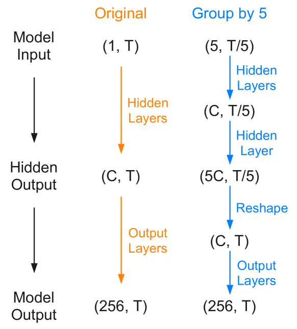
  To further improve the synthesis speed, we applied the grouping mechanism in [30] to the proposed model. As shown in the blue path in Fig. 9, the input sequence with length $T$ is first reshaped and shortened. Each sample in a group is the value of different channels. The method was initially used to build a flow-based model for 1-D speech signals. It has shown effectiveness in improving inference efficiency since the input length is significantly reduced while the channel sizes of the hidden layers remain the same [57, 45]. We denote models using this mechanism as g-$i$, where $i$ indicates the number of samples in a group.

• Tacotron 2 An Tacotron 2 [6] was built as a frontend for text-to-speech synthesis. The model was modified from the public implementation by Nvidia . We applied the reduction factor in [5] to improve convergence speed. The implementation is publicly available .

IV-D Evaluation Metrics

We used four objective and one subjective metrics in the following experiments to evaluate the distortion of the generated speech in different perspectives and the quality under human perception.

• Objective Evaluation We used Mel-cepstral distortion (MCD) [58] to evaluate the distortion in the frequency domain. Mel-cepstrums were first extracted from ground truth and generated speech. Then dynamic time warping (DTW) algorithm was applied to align the features, and the cost of the optimal alignment represented the distortion. To further show the pitch accuracy of generated speech, we calculated the root mean square error of F0 (F0-RMSE). We also calculated the error rate of V/UV flags (V/UV Error), which was the percentage of the frames with mismatched V/UV flags.

• Subjective Evaluation We conducted Mean Opinion Score (MOS) tests to rate the quality of generated speech under human perception. We randomly selected 20 utterances for the evaluation, and each utterance was scored by 20 subjects. The raters were asked to score the samples based on their naturalness on a 1-to-5 scale. A higher score indicate better quality in naturalness.

V Results

Figure 10: Mel-spectrograms of generated speech using ground truth acoustic features ground truth acoustic features from the test set of LJ Speech (LJ050-0241).

V-A Objective Evaluation

In this section, we used different objective metrics to evaluate the efficiency and performance of the proposed methods and other vocoders. All the models were trained using the LJ Speech corpus. We separated 100 utterances as the test set.

V-A1 Model Sizes and Inference Speed

Table I shows the model sizes of different methods and their inference speed. The second column reports the number of model parameters (in millions). Among all methods, Parallel WaveGAN was the smallest in size. The adversarial network [59] enabled the lightweight generator in Parallel WaveGAN to learn effectively with a discriminator. The proposed model had about 30% more parameters than WaveNet and WaveRNN since the network was deeper. The sizes of those with the grouping mechanism (g-5 and g-10) were with more parameters since their channel sizes were 5 times and 10 times larger in the hidden layers, respectively, as shown in the blue path of Fig. 9.

TABLE I: Model sizes and inference speed (w/o and w/ GPU) of different models. For Parallel WaveGAN, only the parameters of the generator are counted.

Model	Size (M)	CPU (kHz)	GPU (kHz)
WaveNet	4.7	0.2	0.1
WaveRNN	4.3	1.1	1.9
Parallel WaveGAN	1.3	20.0	1325.8
Proposed	5.8	8.9	393.1
w/o PF	5.6	9.2	415.6
g-5	7.0	27.9	891.6
g-10	7.3	46.3	1257.0

As for measuring the inference speed, we tested these models using an Intel i7-6700K CPU and an Nvidia 2080Ti GPU. Since the efficiency of non-autoregressive models might be affected by the length of the target speech at the inference stage, we selected 8 utterances with various lengths. The duration of the audio clips ranged from 2 to 10 seconds, and the average duration was 5.8 seconds. The third and fourth columns of Table I shows the generating rate (number of generated samples per second, in kHz) with and without GPU. We concluded our observations as follows:

• The autoregressive models generated speech slow with and without GPU. WaveNet was a deep network with many convolutional layers. It took a lot of computing time in each iteration and could only generate hundreds of samples per second. WaveRNN used two GRUs to replace the convolutional layers, making it faster and more lightweight, but both methods were far from real-time (22 kHz).

• The non-autoregressive method, Parallel WaveGAN, was at 1325.8 kHz and reaches 60 times faster than real-time with GPU. In the case of inference only with CPU, it was still at a rate of 20 kHz. The high efficiency came from Parallel WaveGAN’s lightweight generator and its parallel synthesis architecture.

• The proposed model increased the autoregressive inference speed by changing from the time domain to the frequency domain and the bit precision domain. We also showed in the fourth and fifth rows that using a compact $PF$ to sample signals from posteriorgrams had only a little degradation on speed. The proposed model was 18 times faster than real-time with GPU, shortening the performance gap between autoregressive and non-autoregressive methods. Finally, we measured the rate of the proposed models with the grouping mechanism and showed the mechanism’s effectiveness in improving efficiency. When inference only with CPU, g-5 and g-10 achieved 1.3 and 2.1 times faster than real-time, respectively.

TABLE II: Objective evaluation results of different models when using ground truth acoustic features from the test set of LJ Speech.

Model	MCD	F0-RMSE	V/UV Error
WaveNet	16.89	7.29	6.53
WaveRNN	13.06	3.96	4.57
Parallel WaveGAN	10.54	5.19	6.07
Proposed	8.39	4.44	4.77
w/o PF	11.67	4.29	5.57
g-5	8.51	5.37	5.57
g-10	10.08	5.02	5.40

V-A2 Evaluation Results

We took 38 utterances from the test set of LJ Speech (LJ050-0241$\sim$LJ050-0278) and evaluated the models using different objective metrics. The results are listed in Table II. The proposed models (Proposed, g-5, and g-10) and Parallel WaveGAN had a lower MCD, which indicated the magnitude information was better restored. We attributed the performance to the STFT auxiliary loss [31] since it directly optimized the magnitude distortion in the frequency domain. Regarding F0-RMSE and V/UV Error, WaveRNN outperformed the others, but the difference was not significant since the values of F0 varied at a much larger scale, from hundreds to thousands.

TABLE III: Ablation study on the proposed methods when using ground truth acoustic features from the test set of LJ Speech.

Model	MCD	F0-RMSE	V/UV Error
Proposed	8.39	4.44	4.77
w/o PF	11.67	4.29	5.57
w/o PF, BAR-2	12.04	4.55	5.20
w/o PF, w/o BAR	21.23	4.48	5.24
w/o PF, INV	27.24	8.94	34.73

V-A3 Ablation Study

To show the effects of the proposed methods, we conducted an ablation study. As described in Section III-C, in BAR, the model iteratively predicts the first three bits and then the complete 8-bit signals. We evaluated a model predicting only two bits first and denoted it as BAR-2. INV denotes the model in FAR generating from the subband with the lowest frequency to the one with the highest.

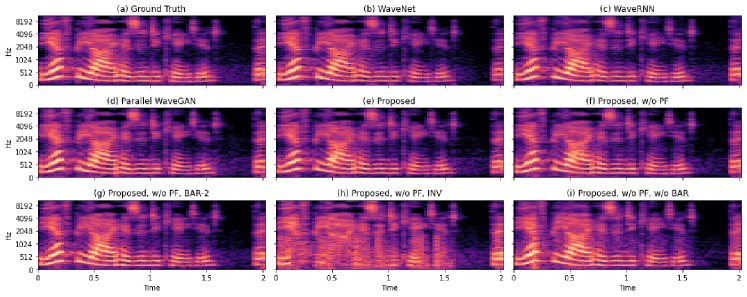
The results are listed in Table III. We found the tendency that the performance degraded while removing PF and BAR. Also, it is evident that INV drastically increased the distortion and error. To visualize the distortion, we plotted Mel-spectrograms generated by different models in Fig. 10. The baseline and proposed models ((b)$\sim$(e)) restored the magnitude information close to the ground truth, While the models in the ablation study ((f)$\sim$(i)) generated utterances with more noise and distortion. The observations from this ablation study showed the importance of the proposed methods and the order to synthesize different subband signals.

V-B Subjective Evaluation

V-B1 Evaluation on Ground Truth Acoustic Features

We randomly selected 20 utterances from the test set of LJ Speech for the subjective evaluation. The MOS results of different models are listed in Table IV. We concluded our observations as follows:

TABLE IV: MOS results of different models when using ground truth acoustic features from the test set of LJ Speech. The scores are reported with 95% confidence intervals.

Model	MOS
WaveNet	3.93$\pm$0.101
WaveRNN	3.85$\pm$0.096
Parallel WaveGAN	3.43$\pm$0.122
Proposed	4.01$\pm$0.098
w/o PF	3.50$\pm$0.108
g-5	3.96$\pm$0.091
g-10	3.88$\pm$0.090
Ground Truth	4.26$\pm$0.087

• Among the baseline models, the autoregressive models bettered the non-autoregressive Parallel WaveGAN. The proposed model outperformed the others and reached a MOS of 4.01, which indicated the quality of the generated utterances was closest to natural human speech.

• Parallel WaveGAN achieved intermediate results in the objective evaluation, and the visualized Mel-spectrogram in Fig. 10 also shows good quality. However, since it was relatively low-quality to the competitive systems, subjects in the MOS test tended to give much lower scores. The audio samples on the demo  page better show the quality of different vocoders.

• The score of the proposed model without PF dropped by 0.5, indicating the importance of PF in synthesizing natural speech. As for the grouping mechanism, the scores of g-5 and g-10 degraded slightly but still close to WaveNet and WaveRNN, showing the ability to improve the synthesis efficiency while preserving the quality.

TABLE V: MOS results of different models when using acoustic features generated from Tacotron 2. The scores are reported with 95% confidence intervals.

Model	MOS
WaveNet	3.57$\pm$0.120
WaveRNN	3.61$\pm$0.096
Parallel WaveGAN	3.59$\pm$0.105
Proposed	3.99$\pm$0.094
g-5	3.85$\pm$0.089
g-10	3.81$\pm$0.091

V-B2 Evaluation on Acoustic Features from Tacotron 2

We combined vocoders with a Tacotron 2 model as complete TTS systems for further evaluation. The Tacotron 2 was trained using the training set of LJ Speech. During inference, we selected 20 sentences from Harvard Sentences [60] as the text input for the systems.

The results are shown in Table V. Compared with the evaluation using ground truth acoustic features, the scores between the baseline methods become closer. We found that features from Tacotron 2 had more distortion than ground truth features. In this case, the autoregressive models, WaveNet and WaveRNN, were unstable, resulting in speech with noise and artifacts. In contrast, Parallel WaveGAN was much more stable regardless of the quality of the input features. As for the proposed models, all three models maintained high quality and outperformed the baseline models by 6$\sim$12%.

TABLE VI: Objective evaluation results of different models when using ground truth acoustic features from speaker bdl and slt in CMU ARCTIC. The vocoders were trained on VCTK corpus.

Model	MCD	F0-RMSE	V/UV Error
bdl (male)
WaveNet	11.24	3.59	9.25
WaveRNN	11.44	2.94	11.43
Parallel WaveGAN	12.61	3.22	7.40
Proposed	8.51	3.05	7.36
slt (female)
WaveNet	10.70	3.84	5.59
WaveRNN	15.77	3.36	2.90
Parallel WaveGAN	11.86	3.97	4.40
Proposed	9.36	3.20	2.60

TABLE VII: MOS results of different models when using ground truth acoustic features from speaker bdl and slt in CMU ARCTIC. The vocoders were trained on VCTK corpus. The scores are reported with 95% confidence intervals.

Model	MOS
WaveNet	3.94$\pm$0.095
WaveRNN	3.62$\pm$0.092
Parallel WaveGAN	3.48$\pm$0.090
Proposed	3.71$\pm$0.099
Ground Truth	4.07$\pm$0.090

TABLE VIII: Objective evaluation results of different models when using ground truth acoustic features from the test set of our 44 kHz internal mandarin speech corpus.

Model	MCD	F0-RMSE	V/UV Error
WaveNet	18.62	31.10	15.43
WaveRNN	22.22	4.59	7.12
Parallel WaveGAN	14.11	9.32	11.06
Proposed	9.07	6.70	6.07

TABLE IX: MOS results of different models when using ground truth acoustic features from the test set of our 44 kHz internal mandarin speech corpus. The scores are reported with 95% confidence intervals.

Model	MOS
WaveNet	3.96$\pm$0.086
WaveRNN	3.82$\pm$0.087
Parallel WaveGAN	2.91$\pm$0.108
Proposed	3.92$\pm$0.091
Ground Truth	4.06$\pm$0.091

V-C Generalization Evaluation

In this section, we studied the generalization abilities of the baseline and proposed models under different situations, including synthesizing speech of unseen speakers and high-fidelity speech with a 44 kHz sampling rate.

V-C1 Generalization to Unseen Speakers

To build a multi-speakers version of the vocoders, we used the VCTK dataset for training. We use utterances from speaker bdl and slt in CMU ARCTIC as a male and a female test set, respectively. For each test set, we took 30 utterances (arctic_b0500$\sim$arctic_b0529) for objective evaluation and randomly selected 10 audio clips for subjective evaluation.

Table VI and Table VII list the results. The tendency of the objective scores between different models is similar to the results in Section V-A. WaveRNN performed slightly worse in MCD, reflected in generated speech with more noise and a lower perceptual score. The MOS results showed that WaveNet generalized best. The proposed model also had a higher score than WaveRNN and Parallel WaveGAN, indicating its ability to generalize to unseen speakers.

V-C2 Generalization to High-Fidelity Dataset

To study the performance when generalization to high-fidelity dataset, we trained the vocoders on our 44 kHz internal Mandarin speech corpus. The acoustic features were extracted using the same parameters as for the 22 kHz corpus, described in Section IV. We took 30 utterances from the test set for objective evaluation and randomly selected 20 utterances for subjective evaluation.

The results are shown in Table VIII and Table IX. The objective evaluation results showed a similar tendency as previous. We found that speech volume from WaveNet varied in the same utterance, leading to worse objective evaluation results. As for the MOS results, utterances from WaveRNN had a bit more noise but were still graded with good scores. Besides, Parallel WaveGAN failed to generated natural results. On the other hand, both WaveNet and the proposed model achieved close scores to the ground truth, indicating their ability to synthesize natural high-fidelity speech.

VI Conclusion

In this paper, we propose novel frequency-wise autoregressive generation (FAR) and bit-wise autoregressive generation (BAR). The former iteratively generates utterances of different frequency subbands, and the latter iteratively generates utterances with different bit precisions. We also applied a post-filter for posterior sampling to further improve the quality. Compared with conventional autoregressive vocoders, the proposed model computes a fixed number of iterations, and the inference time is no longer proportional to the speech length. Consequently, the model possesses high inference efficiency and achieves faster than real-time without GPU acceleration. Besides, the perceptual evaluations also show that the proposed model is able to generate high-quality natural speech under different scenarios.

References

- [1] I. Elias, H. Zen, J. Shen, Y. Zhang, Y. Jia, R. Skerry-Ryan, and Y. Wu, “Parallel tacotron 2: A non-autoregressive neural tts model with differentiable duration modeling,” arXiv preprint arXiv:2103.14574, 2021.
- [2] Y. Ren, C. Hu, X. Tan, T. Qin, S. Zhao, Z. Zhao, and T.-Y. Liu, “Fastspeech 2: Fast and high-quality end-to-end text to speech,” arXiv preprint arXiv:2006.04558, 2020.
- [3] A. v. d. Oord, S. Dieleman, H. Zen, K. Simonyan, O. Vinyals, A. Graves, N. Kalchbrenner, A. Senior, and K. Kavukcuoglu, “Wavenet: A generative model for raw audio,” arXiv preprint arXiv:1609.03499, 2016.
- [4] K. Qian, Y. Zhang, S. Chang, D. Cox, and M. Hasegawa-Johnson, “Unsupervised speech decomposition via triple information bottleneck,” arXiv preprint arXiv:2004.11284, 2020.
- [5] Y. Wang, R. Skerry-Ryan, D. Stanton, Y. Wu, R. J. Weiss, N. Jaitly, Z. Yang, Y. Xiao, Z. Chen, S. Bengio et al., “Tacotron: Towards end-to-end speech synthesis,” arXiv preprint arXiv:1703.10135, 2017.
- [6] J. Shen, R. Pang, R. J. Weiss, M. Schuster, N. Jaitly, Z. Yang, Z. Chen, Y. Zhang, Y. Wang, R. Skerrv-Ryan et al., “Natural tts synthesis by conditioning wavenet on mel spectrogram predictions,” in 2018 IEEE International Conference on Acoustics, Speech and Signal Processing (ICASSP). IEEE, 2018, pp. 4779–4783.
- [7] H. Ze, A. Senior, and M. Schuster, “Statistical parametric speech synthesis using deep neural networks,” in 2013 ieee international conference on acoustics, speech and signal processing. IEEE, 2013, pp. 7962–7966.
- [8] K. Tokuda, Y. Nankaku, T. Toda, H. Zen, J. Yamagishi, and K. Oura, “Speech synthesis based on hidden markov models,” Proceedings of the IEEE, vol. 101, no. 5, pp. 1234–1252, 2013.
- [9] N. Kalchbrenner, E. Elsen, K. Simonyan, S. Noury, N. Casagrande, E. Lockhart, F. Stimberg, A. Oord, S. Dieleman, and K. Kavukcuoglu, “Efficient neural audio synthesis,” in International Conference on Machine Learning. PMLR, 2018, pp. 2410–2419.
- [10] M. Morise, F. Yokomori, and K. Ozawa, “World: a vocoder-based high-quality speech synthesis system for real-time applications,” IEICE TRANSACTIONS on Information and Systems, vol. 99, no. 7, pp. 1877–1884, 2016.
- [11] H. Kawahara, J. Estill, and O. Fujimura, “Aperiodicity extraction and control using mixed mode excitation and group delay manipulation for a high quality speech analysis, modification and synthesis system STRAIGHT,” in Second International Workshop on Models and Analysis of Vocal Emissions for Biomedical Applications, 2001.
- [12] Z. Wu, O. Watts, and S. King, “Merlin: An open source neural network speech synthesis system.” in SSW, 2016, pp. 202–207.
- [13] D. Griffin and J. Lim, “Signal estimation from modified short-time fourier transform,” IEEE Transactions on Acoustics, Speech, and Signal Processing, vol. 32, no. 2, pp. 236–243, 1984.
- [14] Y. Taigman, L. Wolf, A. Polyak, and E. Nachmani, “Voiceloop: Voice fitting and synthesis via a phonological loop,” arXiv preprint arXiv:1707.06588, 2017.
- [15] J.-c. Chou, C.-c. Yeh, H.-y. Lee, and L.-s. Lee, “Multi-target voice conversion without parallel data by adversarially learning disentangled audio representations,” arXiv preprint arXiv:1804.02812, 2018.
- [16] C.-c. Yeh, P.-c. Hsu, J.-c. Chou, H.-y. Lee, and L.-s. Lee, “Rhythm-flexible voice conversion without parallel data using cycle-gan over phoneme posteriorgram sequences,” in 2018 IEEE Spoken Language Technology Workshop (SLT). IEEE, 2018, pp. 274–281.
- [17] A. T. Liu, P.-c. Hsu, and H.-y. Lee, “Unsupervised end-to-end learning of discrete linguistic units for voice conversion,” arXiv preprint arXiv:1905.11563, 2019.
- [18] C.-M. Chien, J.-H. Lin, C.-y. Huang, P.-c. Hsu, and H.-y. Lee, “Investigating on incorporating pretrained and learnable speaker representations for multi-speaker multi-style text-to-speech,” in ICASSP 2021-2021 IEEE International Conference on Acoustics, Speech and Signal Processing (ICASSP). IEEE, 2021, pp. 8588–8592.
- [19] K. Qian, Y. Zhang, S. Chang, X. Yang, and M. Hasegawa-Johnson, “Autovc: Zero-shot voice style transfer with only autoencoder loss,” in International Conference on Machine Learning. PMLR, 2019, pp. 5210–5219.
- [20] Z.-H. Ling, Y. Ai, Y. Gu, and L.-R. Dai, “Waveform modeling and generation using hierarchical recurrent neural networks for speech bandwidth extension,” IEEE/ACM Transactions on Audio, Speech, and Language Processing, vol. 26, no. 5, pp. 883–894, 2018.
- [21] W. B. Kleijn, A. Storus, M. Chinen, T. Denton, F. S. Lim, A. Luebs, J. Skoglund, and H. Yeh, “Generative speech coding with predictive variance regularization,” in ICASSP 2021-2021 IEEE International Conference on Acoustics, Speech and Signal Processing (ICASSP). IEEE, 2021, pp. 6478–6482.
- [22] A. Polyak, Y. Adi, J. Copet, E. Kharitonov, K. Lakhotia, W.-N. Hsu, A. Mohamed, and E. Dupoux, “Speech resynthesis from discrete disentangled self-supervised representations,” arXiv preprint arXiv:2104.00355, 2021.
- [23] J. Lorenzo-Trueba, T. Drugman, J. Latorre, T. Merritt, B. Putrycz, R. Barra-Chicote, A. Moinet, and V. Aggarwal, “Towards achieving robust universal neural vocoding,” arXiv preprint arXiv:1811.06292, 2018.
- [24] P.-c. Hsu, C.-h. Wang, A. T. Liu, and H.-y. Lee, “Towards robust neural vocoding for speech generation: A survey,” arXiv preprint arXiv:1912.02461, 2019.
- [25] Y. Jiao, A. Gabryś, G. Tinchev, B. Putrycz, D. Korzekwa, and V. Klimkov, “Universal neural vocoding with parallel wavenet,” in ICASSP 2021-2021 IEEE International Conference on Acoustics, Speech and Signal Processing (ICASSP). IEEE, 2021, pp. 6044–6048.
- [26] Z. Jin, A. Finkelstein, G. J. Mysore, and J. Lu, “Fftnet: A real-time speaker-dependent neural vocoder,” in 2018 IEEE International Conference on Acoustics, Speech and Signal Processing (ICASSP). IEEE, 2018, pp. 2251–2255.
- [27] J.-M. Valin and J. Skoglund, “Lpcnet: Improving neural speech synthesis through linear prediction,” in ICASSP 2019-2019 IEEE International Conference on Acoustics, Speech and Signal Processing (ICASSP). IEEE, 2019, pp. 5891–5895.
- [28] A. Oord, Y. Li, I. Babuschkin, K. Simonyan, O. Vinyals, K. Kavukcuoglu, G. Driessche, E. Lockhart, L. Cobo, F. Stimberg et al., “Parallel wavenet: Fast high-fidelity speech synthesis,” in International conference on machine learning. PMLR, 2018, pp. 3918–3926.
- [29] W. Ping, K. Peng, and J. Chen, “Clarinet: Parallel wave generation in end-to-end text-to-speech,” arXiv preprint arXiv:1807.07281, 2018.
- [30] R. Prenger, R. Valle, and B. Catanzaro, “Waveglow: A flow-based generative network for speech synthesis,” in ICASSP 2019-2019 IEEE International Conference on Acoustics, Speech and Signal Processing (ICASSP). IEEE, 2019, pp. 3617–3621.
- [31] R. Yamamoto, E. Song, and J.-M. Kim, “Parallel wavegan: A fast waveform generation model based on generative adversarial networks with multi-resolution spectrogram,” in ICASSP 2020-2020 IEEE International Conference on Acoustics, Speech and Signal Processing (ICASSP). IEEE, 2020, pp. 6199–6203.
- [32] N. Chen, Y. Zhang, H. Zen, R. J. Weiss, M. Norouzi, and W. Chan, “Wavegrad: Estimating gradients for waveform generation,” arXiv preprint arXiv:2009.00713, 2020.
- [33] A. v. d. Oord, N. Kalchbrenner, O. Vinyals, L. Espeholt, A. Graves, and K. Kavukcuoglu, “Conditional image generation with pixelcnn decoders,” arXiv preprint arXiv:1606.05328, 2016.
- [34] D. P. Kingma, T. Salimans, R. Jozefowicz, X. Chen, I. Sutskever, and M. Welling, “Improving variational inference with inverse autoregressive flow,” arXiv preprint arXiv:1606.04934, 2016.
- [35] D. P. Kingma and P. Dhariwal, “Glow: Generative flow with invertible 1x1 convolutions,” arXiv preprint arXiv:1807.03039, 2018.
- [36] K. Kumar, R. Kumar, T. de Boissiere, L. Gestin, W. Z. Teoh, J. Sotelo, A. de Brébisson, Y. Bengio, and A. Courville, “Melgan: Generative adversarial networks for conditional waveform synthesis,” arXiv preprint arXiv:1910.06711, 2019.
- [37] T. Okamoto, K. Tachibana, T. Toda, Y. Shiga, and H. Kawai, “Subband wavenet with overlapped single-sideband filterbanks,” in 2017 IEEE Automatic Speech Recognition and Understanding Workshop (ASRU). IEEE, 2017, pp. 698–704.
- [38] T. Okamoto, T. Toda, Y. Shiga, and H. Kawai, “Improving fftnet vocoder with noise shaping and subband approaches,” in 2018 IEEE Spoken Language Technology Workshop (SLT). IEEE, 2018, pp. 304–311.
- [39] Q. Tian, Z. Zhang, H. Lu, L.-H. Chen, and S. Liu, “Featherwave: An efficient high-fidelity neural vocoder with multi-band linear prediction,” arXiv preprint arXiv:2005.05551, 2020.
- [40] T. Nguyen, “Near-perfect-reconstruction pseudo-qmf banks,” IEEE Transactions on Signal Processing, vol. 42, no. 1, pp. 65–76, 1994.
- [41] J. Kong, J. Kim, and J. Bae, “Hifi-gan: Generative adversarial networks for efficient and high fidelity speech synthesis,” arXiv preprint arXiv:2010.05646, 2020.
- [42] J. Chorowski, R. J. Weiss, S. Bengio, and A. van den Oord, “Unsupervised speech representation learning using wavenet autoencoders,” IEEE/ACM transactions on audio, speech, and language processing, vol. 27, no. 12, pp. 2041–2053, 2019.
- [43] D. Rethage, J. Pons, and X. Serra, “A wavenet for speech denoising,” in 2018 IEEE International Conference on Acoustics, Speech and Signal Processing (ICASSP). IEEE, 2018, pp. 5069–5073.
- [44] D. Misra, “Mish: A self regularized non-monotonic neural activation function,” arXiv preprint arXiv:1908.08681, 2019.
- [45] P.-c. Hsu and H.-y. Lee, “Wg-wavenet: Real-time high-fidelity speech synthesis without gpu,” arXiv preprint arXiv:2005.07412, 2020.
- [46] S. Takaki, T. Nakashika, X. Wang, and J. Yamagishi, “Stft spectral loss for training a neural speech waveform model,” in ICASSP 2019-2019 IEEE International Conference on Acoustics, Speech and Signal Processing (ICASSP). IEEE, 2019, pp. 7065–7069.
- [47] S. Takaki, H. Kameoka, and J. Yamagishi, “Training a neural speech waveform model using spectral losses of short-time fourier transform and continuous wavelet transform,” arXiv preprint arXiv:1903.12392, 2019.
- [48] S. Ö. Arık, H. Jun, and G. Diamos, “Fast spectrogram inversion using multi-head convolutional neural networks,” IEEE Signal Processing Letters, vol. 26, no. 1, pp. 94–98, 2018.
- [49] Q. Tian, Y. Chen, Z. Zhang, H. Lu, L. Chen, L. Xie, and S. Liu, “Tfgan: Time and frequency domain based generative adversarial network for high-fidelity speech synthesis,” arXiv preprint arXiv:2011.12206, 2020.
- [50] K. Ito and L. Johnson, “The lj speech dataset,” https://keithito.com/LJ-Speech-Dataset/, 2017.
- [51] J. Yamagishi, C. Veaux, K. MacDonald et al., “Cstr vctk corpus: English multi-speaker corpus for cstr voice cloning toolkit,” 2017.
- [52] J. Kominek and A. W. Black, “The cmu arctic speech databases,” in Fifth ISCA workshop on speech synthesis, 2004.
- [53] A. Paszke, S. Gross, F. Massa, A. Lerer, J. Bradbury, G. Chanan, T. Killeen, Z. Lin, N. Gimelshein, L. Antiga, A. Desmaison, A. Kopf, E. Yang, Z. DeVito, M. Raison, A. Tejani, S. Chilamkurthy, B. Steiner, L. Fang, J. Bai, and S. Chintala, “Pytorch: An imperative style, high-performance deep learning library,” in Advances in Neural Information Processing Systems 32, H. Wallach, H. Larochelle, A. Beygelzimer, F. d'Alché-Buc, E. Fox, and R. Garnett, Eds. Curran Associates, Inc., 2019, pp. 8024–8035. [Online]. Available: http://papers.neurips.cc/paper/9015-pytorch-an-imperative-style-high-performance-deep-learning-library.pdf
- [54] D. P. Kingma and J. Ba, “Adam: A method for stochastic optimization,” arXiv preprint arXiv:1412.6980, 2014.
- [55] J. Yang, J. Lee, Y. Kim, H. Cho, and I. Kim, “Vocgan: A high-fidelity real-time vocoder with a hierarchically-nested adversarial network,” arXiv preprint arXiv:2007.15256, 2020.
- [56] L. Wright, “Ranger - a synergistic optimizer.” https://github.com/lessw2020/Ranger-Deep-Learning-Optimizer, 2019.
- [57] B. Zhai, T. Gao, F. Xue, D. Rothchild, B. Wu, J. E. Gonzalez, and K. Keutzer, “Squeezewave: Extremely lightweight vocoders for on-device speech synthesis,” arXiv preprint arXiv:2001.05685, 2020.
- [58] R. Kubichek, “Mel-cepstral distance measure for objective speech quality assessment,” in Proceedings of IEEE Pacific Rim Conference on Communications Computers and Signal Processing, vol. 1. IEEE, 1993, pp. 125–128.
- [59] I. Goodfellow, J. Pouget-Abadie, M. Mirza, B. Xu, D. Warde-Farley, S. Ozair, A. Courville, and Y. Bengio, “Generative adversarial nets,” Advances in neural information processing systems, vol. 27, 2014.
- [60] E. Rothauser, “Ieee recommended practice for speech quality measurements,” IEEE Trans. on Audio and Electroacoustics, vol. 17, pp. 225–246, 1969.