Optimal Decision Rules when Payoffs are Partially Identified111 We are grateful to X. Chen, L. Hansen, C. Manski, J. Porter, Q. Vuong, and E. Vytlacil and participants in various seminars for helpful comments and suggestions. The theory and methodology developed in this paper is based on and supersedes the preprint arXiv:2011.03153 (Christensen et al., 2020). This material is based upon work supported by the National Science Foundation under Grants No. SES-1919034 (Christensen), SES-1625586 (Moon), and SES-1851634 (Schorfheide).
Abstract
We derive optimal statistical decision rules for discrete choice problems when payoffs depend on a partially-identified parameter and the decision maker can use a point-identified parameter to deduce restrictions on . Leading examples include optimal treatment choice under partial identification and optimal pricing with rich unobserved heterogeneity. Our optimal decision rules minimize the maximum risk or regret over the identified set of payoffs conditional on and use the data efficiently to learn about . We discuss implementation of optimal decision rules via the bootstrap and Bayesian methods, in both parametric and semiparametric models. We provide detailed applications to treatment choice and optimal pricing. Using a limits of experiments framework, we show that our optimal decision rules can dominate seemingly natural alternatives. Our asymptotic approach is well suited for realistic empirical settings in which the derivation of finite-sample optimal rules is intractable.
Keywords: Model uncertainty, statistical decision theory, partial identification, treatment assignment, revealed preference
JEL codes: C10, C18, C21, C44, D81
1 Introduction
Many important policy decisions involve discrete choices. Examples include whether or not to treat an aggregate population or large sub-population, firm or worker decisions at the extensive margin, and pricing policies when, in practice, prices must be expressed in whole currency units. Suppose a decision maker must choose a policy from a discrete choice set. The decision maker has data that may be used to bound, but not point identify, the payoffs associated with some choices. For instance, the decision maker may be deciding whether or not to assign treatment based on observational data which is sufficient to bound, but not point identify, the average treatment effect. How should they proceed?
In this paper, we propose an approach for making optimal discrete statistical (i.e., data-driven) decisions when the payoffs associated with some choices are only partially identified. In the model described in Section 3, the decision maker observes data which may be used to learn about a vector of parameters . The decision maker then chooses a policy from among a discrete set. The distribution of payoffs associated with the different policies is indexed by a structural parameter . A key assumption underlying the analysis in this paper is that is possibly set-identified, but the parameters may be used to deduce restrictions on . The decision maker therefore confronts both ambiguity (the payoff distribution is not point-identified) and statistical uncertainty ( must be estimated from the data).
We propose a theory of optimal statistical decision making in this setting, building on a line of research going back to Manski (2000). We depart from this body of work by adopting a minimax approach to handle the ambiguity that arises from the partial identification of conditional on and average (or integrated) risk minimization to efficiently estimate . This asymmetric treatment of parameters is in the spirit of the generalized Bayes-minimax principle of Hurwicz (1951). The resulting optimal decision rules are “robust” in the sense that they minimize maximum risk or regret over the identified set for conditional on , and use the data to learn efficiently about features of germane to the choice problem.
In contrast with existing approaches, our optimal decision rules can be implemented very easily in realistic empirical settings via the bootstrap or (quasi-)Bayesian methods, for both parametric and semiparametric models. To describe the implementation, fix any choice and consider its maximum risk (or regret) over conditional on . The maximum risk (or regret) is averaged across the bootstrap distribution for an efficient estimator of , a posterior distribution for (in parametric models), or a quasi-posterior based on a limited-information criterion for (in semiparametric models). Our optimal decision is then to simply to choose whatever choice has smallest average maximum risk (or regret). We show how to implement optimal decisions in the context of two applications, which we use as running examples. The first considers treatment assignment under partial identification of the average treatment effect (ATE). The second considers optimal pricing in an environment with rich unobserved heterogeneity, where revealed preference arguments may be used to bound, but not point identify, demand responses under counterfactual prices. In both examples, the maximum risk (or regret) of different choices is available in closed form or can be computed by solving a standard optimization problem, e.g., a linear program. Though simple, we provide a formal (frequentist) asymptotic efficiency theory to justify our approach.
To elaborate on practicality a little, consider the two competing paradigms: Bayes and minimax. A Bayes decision requires specifying a prior on the parameter space for , computing the posterior for having observed the data, then choosing the decision that minimizes posterior risk. A common criticism of Bayes decisions (see, e.g., Manski (2021)) is that they are only justified if one can elicit a credible subjective prior, which can be difficult in practice, and that the resulting decision will depend, to some extent, on the decision maker’s choice of prior. This is true under both point- and partial identification. But this problem is more pronounced under partial identification because the decision maker’s choice of prior for the partially identified parameter is not updated by the data (e.g., Moon and Schorfheide (2012)). Thus, the resulting decision will depend, even asymptotically, on the decision maker’s choice of prior. By contrast, our (quasi-)Bayesian implementations only require specifying a prior for the point-identified parameter and our decisions are asymptotically independent of the choice of prior. Moreover, our bootstrap implementations sidestep choice of prior altogether.
Minimax decisions are those which maximize risk (or regret) uniformly over . While minimaxity may be desirable, it is often not feasible. That is, to derive minimax decisions one often has to make strong assumptions on the data-generating process (e.g., Gaussian with known variance) and restrict the dependence of payoffs on model parameters to be of a very simple form. Indeed, we are not aware of any work deriving a minimax treatment rule under partial identification even in the simplest case of a binary outcome and binary treatment when randomization is not permitted and bounds on the ATE must be estimated from data. Algorithms such as that of Chamberlain (2000) may be used to compute approximate minimax decisions, but the performance gap between these and the true minimax decision can be difficult to quantify. Adopting a minimax approach with respect to and an average risk minimization approach with respect to lends a great deal of tractability, allowing us to derive optimal rules for a very broad class of empirically relevant settings where minimax rules are intractable. In particular, our approach does not require strong parametric assumptions on the data-generating process, accommodating semiparametric models, and allows complicated dependence of payoffs on model parameters.
Sections 4 and 5 present optimality results for decisions based on parametric and semiparametric models, respectively. For parametric models, our efficiency criterion extends the asymptotic average risk criterion introduced by Hirano and Porter (2009) for point-identified settings to partially identified settings. We further extend this notion to semiparametric models via a least-favorable parametric submodel. Both of these extensions represent new contributions to the literature on asymptotic efficiency for statistical decision rules. Our main results show formally that the proposed (quasi-)Bayesian implementation is optimal under our asymptotic efficiency criterion. Moreover, any decision rule that is asymptotically equivalent to the Bayes implementation is optimal as well. Most importantly, this includes an implementation that replaces averaging under a (quasi-)posterior by averaging under a bootstrap approximation of the sampling distribution of an efficient estimator of , in cases in which these two distributions are asymptotically equivalent.
Importantly, we show asymptotic equivalence to the proposed Bayesian or bootstrap implementations is in fact necessary for optimality: any decision whose asymptotic behavior is different from these is sub-optimal. Hence, it follows from our necessity result that “plug-in rules”, which plug an efficient estimator into the oracle decision rule if were known, can perform sub-optimally. Manski (2021, 2022) refers to plug-in rules as “as-if” optimization, because the estimated parameters are treated as if they are the true parameters. Manski (2021, 2022) shows in numerical experiments that plug-in rules may perform poorly under finite-sample minimax regret criteria. Our necessity result provides a complementary and quite general theoretical explanation for why plug-in rules may perform poorly, albeit under a different (but related) optimality criterion to that of Manski (2021, 2022).222For the intuition, consider a treatment assignment problem under partial identification of the ATE. Oracle rules depend on a robust welfare contrast formed from bounds on the ATE. The bounds are non-smooth functions of in many empirically relevant settings reviewed in Section 8 and include intersection bounds, nonseparable panel data models, and bounds based on extrapolating IV estimands. This non-smoothness leads to a failure of the -method that breaks the asymptotic equivalence between plug-in rules, which depend on , and optimal rules, which depend on the average of across a bootstrap or posterior distribution.
In Section 2 we present an empirical application based on Ishihara and Kitagawa (2021) in which a decision maker decides whether or not to adopt a job-training program based on several RCT estimates and their standard errors from other studies. Intersection bounds are derived by extrapolating multiple studies. Our optimal decision produces different treatment recommendations than the plug-in rule for some sub-populations. In Section 4 we show this difference is explained clearly through our optimality theory and necessity result.
Our application to optimal pricing is presented in Section 7. The problem we study is similar to the problem of robust monopoly pricing studied by Bergemann and Schlag (2011), in which a decision maker is choosing to set a price but faces ambiguity about the true distribution of demand. As in Bergemann and Schlag (2011), we assume the decision maker has a preference for robustness. However, we use revealed preference demand theory to derive bounds on demand, rather than assuming true demand is in a neighborhood of a pre-specified distribution. Moreover, in our setting the decision maker does not know bounds on demand ex ante but must instead estimate bounds from data. This application builds on prior work on revealed-preference demand theory, including Blundell et al. (2007, 2008), Blundell et al. (2014, 2017), Hoderlein and Stoye (2015), Manski (2007b, 2014), and Kitamura and Stoye (2018, 2019). These works are primarily concerned with testing rationality or deriving bounds on demand. We instead focus on using bounds to solve an optimal pricing problem, and using demand data efficiently in that context.
This paper complements prior work on treatment assignment under partial identification, including Manski (2000, 2007a, 2020, 2021, 2022), Chamberlain (2011), Stoye (2012), Russell (2020), Ishihara and Kitagawa (2021), and Yata (2021). Except for Chamberlain (2011), these works seek decision rules that are optimal under finite-sample minimax regret criteria. We depart from these works in two respects. First, our local asymptotic framework enables us to approximate the finite-sample problem faced by the decision maker without having to explicitly solve the finite-sample problem, which may be intractable in many important applications. This allows us to relax restrictive parametric assumptions on the data-generating process (e.g. Gaussianity) that are typically imposed to derive finite-sample rules. It also allows us to accommodate a much broader class of data-generating processes, including semiparametric models. Our optimality results apply to settings where the decision maker cannot confidently assert that the data are drawn from a given parametric model, or where bounds on the ATE are estimated using a vector of moments or summary statistics (e.g. regression or IV estimates from observational studies) whose finite-sample distribution is unknown.333Finite-sample results are sometimes developed for this case assuming Gaussianity of the statistics, by arguing that the studies are sufficiently large that the sampling distribution of the statistics is approximately normal. In these cases, it seems logically consistent to use a large-sample optimality criterion. Second, except for Chamberlain (2011), these works use optimality criteria that (in our notation) are minimax over , whereas our criterion is minimax over the partially-identified parameter and averages over the point-identified parameter , reflecting the asymmetric parameterization of the problem.
Our approach is closely related to the multiple priors framework of Gilboa and Schmeidler (1989) and robust Bayes (or -minimax) decision making (Robbins, 1951; Berger, 1985) in partially identified models. See Giacomini et al. (2021) for a recent review. Our paper makes several novel contributions in connection with -minimax decisions. First, for parametric models, we provide a large-sample frequentist justification for these types of decision rules, which complements the usual finite-sample robust Bayes justification. Second, we show this optimality carries over to (i) bootstrap-based decisions and (ii) quasi-Bayes decisions in semiparametric models. In these latter cases the decisions we derive are not -minimax decisions, but rather have a purely frequentist justification.
The remainder of the paper is structured as follows. Section 2 presents the empirical application to treatment assignment based on extrapolating meta-analyses. Section 3 outlines our framework and derives the optimal decisions. Optimality theory is presented in Sections 4 and 5. Section 6 discusses connections with robust Bayes decisions. Further applications to optimal pricing and treatment assignment are discussed in Sections 7 and 8. Finally, Section 9 concludes. Technical assumptions and proofs are relegated to the Appendix.
2 Motivating Example: Treatment Assignment
The Treatment Assignment Problem. Consider a social planner who is choosing whether or not to introduce a treatment in a target population. For concreteness, suppose that the the social planner does not know the target population’s average treatment effect (ATE) but, as in Manski (2020) and Ishihara and Kitagawa (2021, hereafter IK), they observe a meta-analysis consisting of estimates of the ATE in several related populations , their standard errors , characteristics of the related populations, and characteristics of the target population. The parameters may be used to construct bounds on the ATE of the target population, which we denote by . Here is the treatment effect associated with an individual and defined as , where is the outcome under treatment and the outcome in the absence of treatment.
As an empirical illustration, we revisit Example 2 of IK. The authors consider a subset of studies form the database of Card et al. (2017), each of which is an RCT looking at the impact of job training programs on employment. Studies are implemented in a number of different countries and in groups that differ by characteristics consisting of gender (males, females, or both), age (youths, adults, or both), OECD membership status, GDP growth (standardized) and unemployment (standardized). We consider the hypothetical question of whether to roll out a job-training program in two populations: German male youths in 2010 and German female youths in 2010 (with GDP growth of 3.48% and an unemployment rate of 9.45%).
IK bound the difference between the treatment effect in the target population and in the related population as
| (1) |
where is a pre-specified constant. Hence we obtain the bounds
| (2) |
where . We will refer to as the identifiable reduced-form parameter. It is assumed to be estimable from the data. The identified set for as a function of given by (2) is . More generally, the following analysis applies in any context where is partially identified and bounds and on are known up to a finite-dimensional, identifiable parameter . How should the social planner use the ATE bounds and , the estimates , and their standard errors to inform whether or not to treat the target population?
Oracle Decision. Following Manski (2000, 2004), it is common to derive treatment rules under a utilitarian social welfare function that is linear in the target population’s ATE:
where indicates treatment. The welfare function is maximized by the treatment decision , where is the indicator function that is equal to one if the condition is satisfied and zero otherwise. Following Manski (2000, 2004), we subsequently use the regret criterion
| (3) |
Failure to treat () incurs zero regret when , otherwise the regret is . Similarly, treating () incurs zero regret when , otherwise the regret is .
If the social planner knew , then they could choose the decision that minimizes maximum regret over as follows. As non-treatment () incurs regret when and zero otherwise, the maximum regret associated with choice is
where . Similarly, as treatment () incurs regret when and zero otherwise, the maximum regret associated with choice is
where . This leads to the oracle decision that assigns treatment if the robust welfare contrast
is non-negative, and non-treatment otherwise:
| (4) |
Efficient Feasible Implementation. The oracle rule is an infeasible first-best as it requires knowledge of the true . In practice is unknown and any practical rule must also confront sampling uncertainty about . One option is to simply plug the ATE estimates into the oracle decision, which leads to the plug-in rule
| (5) |
However, this rule does not account for the precision with which is estimated. Manski (2022) explores how different estimates of model parameters affects the performance of plug-in rules.
We develop an efficiency theory to guide decision-making in situations such as these where a payoff-relevant parameter is partially identified and its identified set is indexed by a parameter which can be estimated from data. In our empirical illustration the efficient treatment assignment procedure can be implemented in two steps with the following quasi-Bayesian procedure.
The first step consists of the construction of a limited-information posterior distribution for . We assume that sample sizes are sufficiently large, such that the distribution of the ATE estimator is approximately . The estimates are also independent as they come from independent RCTs. Following Doksum and Lo (1990) and Kim (2002), we combine the limited information quasi-likelihood for with a flat prior for to obtain a quasi posterior for , where denotes a diagonal matrix with down its leading diagonal.
In the second step, we average the robust welfare contrast across the quasi-posterior for to compute its quasi-posterior mean . This is implemented by simply drawing independent , computing , then averaging across a large number of draws. The efficient decision is then to treat if the quasi-posterior mean is non-negative, and not treat otherwise:
| (6) |
Later we show under the optimality criterion in Section 4, this decision is more efficient than the plug-in rule as it takes into account the sampling uncertainty in the ATE estimates .
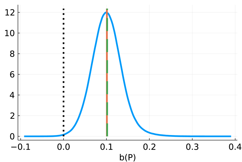
Using the data set, we compute the optimal decision as described above. For this, we increase the Lipschitz constant in (1) from in IK to so that the bounds on are non-empty. Figures 1(a) and 1(b) plot the quasi-posterior distribution of the robust welfare contrast for males and females, respectively, for . Both figures display the mean whose sign determines the optimal treatment decision in (6). We also display the plug-in value whose sign determines the plug-in rule in (5).
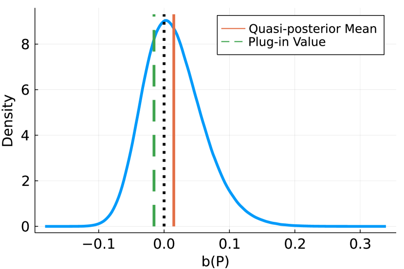
In Figure 1(a) (male youths) we see that the distribution has a mode located at zero and a pronounced right-skew. Recall that the lower bound is . When evaluated at the , the largest value of is (corresponding to a US study) and the second-largest is (corresponding to a Brazilian study). As the maximum is not well separated relative to sampling uncertainty (the average across the studies is ), the distribution of the lower bound is right-skewed because it behaves like a maximum of two Gaussians. The upper bound is less skewed because the minimum (which corresponds to a Colombian study) is better separated. As a consequence of this asymmetry, the mean is positive and the optimal decision is to treat. By contrast, the plug-in value is negative so the plug-in decision is to not treat. In Section 4 we show this difference between the two rules is as predicted by our optimality theory.
The situation is different for female youths (Figure 1(b)). Here the minima and maxima are relatively better separated, so the distribution of for is close to Gaussian. In consequence, the mean and the plug-in value are almost identical, and the optimal and plug-in decisions are both to treat.
3 Optimal Decisions and Their Implementation
We now move beyond this illustration to present our general approach. We begin in Section 3.1 by stating the decision problem. It features a partially-identified payoff-relevant parameter and a point-identified parameter that determines the identified set for . Many empirically relevant examples are covered by our framework: see Sections 7 and 8 for further applications to treatment assignment and optimal pricing and our earlier working paper Christensen et al. (2020) for application to forecasting. We develop our concept of optimal decision rules in Section 3.2. Bayesian and bootstrap implementations are presented in Sections 3.3 and 3.4. Later in Section 6 we interpret our approach in the context of a two-player zero-sum game and relate it to the literature on robust Bayes decision making.
3.1 Decision Problem
A decision maker (DM) observes taking values in a sample space . For instance, may be a random sample of size with denoting the -fold product distribution over independent random vectors . Alternatively, may be a vector of estimates or summary statistics (e.g., OLS or IV estimates) with denoting the sampling distribution of . The distribution from which is drawn is indexed by an unknown reduced-form parameter . To simplify exposition, in this section we will be exclusively concerned with parametric models for . Our approach extends naturally to semiparametric models, as discussed in Section 5.
After observing , the DM chooses an element from a finite set . The DM’s statistical decision rule maps realizations of the data into choices.444We use the subscript to denote that a decision rule may also depend on sample size . The DM incurs risk (negative expected utility)
from choice , where the expectation is taken with respect to a random vector
drawn independently of . The distribution and expectation can be conditional on covariates; we suppress this to simplify notation. The distribution is indexed by a structural parameter , as described in detail below. We may interpret the expectation as a forward-looking expectation over a random outcome, or a cross-sectional average in a social planner’s problem. Our notation encompasses welfare regret by setting
for a welfare function . We therefore do not distinguish between “risk” and “regret” in what follows, except when referring to functional forms for .
A key assumption underlying the analysis in this paper is that is possibly set-identified. That is, the most that the DM can infer about is that , where is a known set-valued mapping from the reduced-form parameter space to the structural parameter space. So while can be used to learn about , it contains no information about the identity of the true within .
Example: Treatment Assignment.
Consider the setup from Section 2. Here is a binary treatment indicator. The structural parameter is the ATE. The risk (i.e., regret) is given in display (3). Suppose the DM observes data or summary statistics that may be used to construct bounds and on as a function of . In the application from Section 2, the statistics were the vector of estimated ATEs , is their sampling distribution, the reduced-form parameter is the vector of ATEs , and and are given in (2). We review other methods for constructing bounds in different empirical settings in Section 8. The identified set is .
3.2 Optimality Criterion
We now define our optimality criterion. Our setup features two types of parameters: a point-identified parameter and a set-identified parameter that affects risk. We adopt a minimax approach to handle the ambiguity that arises from the partial identification of conditional on and average (or integrated) risk minimization to efficiently estimate . Our asymmetric treatment of parameters is in the spirit of Hurwicz (1951); we discuss the connection in more detail in Section 3.3. We first consider the case in which is known and then extend the analysis to the case of unknown , which will lead us to the definition of our optimality concept.
Known .
First suppose that is known to the DM. To handle the ambiguity about , the DM evaluates choices by their maximum risk
| (7) |
The minimax decision for known is
if the argmin is unique, otherwise is chosen randomly from . The choice can be interpreted as the equilibrium in a two-player zero-sum game in which an adversarial “nature” chooses in response to the DM’s choice of to minimize . We refer to as the oracle decision, as it represents the DM’s optimal choice if was known. The oracle decision is an infeasible first-best, as in any application will need to be estimated from data. Nevertheless, the oracle decision is a useful benchmark, as its maximum risk, namely , is a lower bound on the minimax risk when is unknown.
Unknown .
When the DM does not know , the DM’s decision will be data-dependent. For a decision rule , the DM incurs frequentist (or average) maximum risk
| (8) |
where denotes expectation with respect to . Our goal is to construct decision rules that use the data efficiently, in the sense that their average maximum risk is as close to that of the oracle over a range of data-generating processes.
Following Hirano and Porter (2009), we use a local asymptotic framework based on perturbations to the data-generating process of the same order as sampling variation. The idea of this asymptotic framework is that, although asymptotic, it should well approximate the DM’s finite-sample problem in which is unknown.
Formally, fix any limiting and let denote its local perturbation by for a sample of size . For the asymptotic analysis it is convenient to express the frequentist maximum risk in excess of the oracle risk (the infeasible first-best) when is the true reduced-form parameter. We scale the excess risk by to ensure the large-sample limit is not degenerate.
| (9) |
which is non-negative, and where the limit exists for large class of decision rules whose asymptotic behavior is well-defined—see Section 4. This asymptotic frequentist maximum risk depends on the perturbation parameter . Integrating over yields the asymptotic average maximum risk criterion:
| (10) |
We define optimality as follows:
Definition 1
A sequence of decision rules is optimal if
Remark 3.1
An alternative is to take the maximum over rather than integrating over as in (10), which has the downside that optimal decisions are computationally intractable in most empirically relevant settings. By contrast, to implement optimal decisions under our criterion (10), the DM only needs to be able to compute maximum risk as a function of for each choice . As we are considering decision problems in which may be non-smooth in , different optimality concepts generally lead to different decisions.
In the remainder of this section we present a Bayesian implementation and a bootstrap implementation of optimal decisions.
3.3 Bayesian Interpretation and Implementation
Let denote a strictly positive, smooth density on . Integrating the frequentist maximum risk criterion (8) across using yields the integrated maximum risk criterion
| (11) |
After observing , the DM can form a posterior for . Standard arguments (e.g. Wald, 1950, Chapter 5.1) imply that the integrated maximum risk can be minimized by minimizing the posterior maximum risk
| (12) |
with respect to for almost every realization of the data. This leads to the Bayes rule
| (13) |
if the argmin is unique, otherwise is chosen randomly from . We include as an argument to indicate that the decision depends on in finite samples.
We formally prove in Section 4 that Bayes decisions are optimal under criterion (10) for any prior whose density is strictly positive and smooth at . To see the connection between (11) and (10), use a change-of-variables to express the prior for as . This prior becomes uniform as , which is the weight function underlying (10).
Example: Treatment Assignment.
Recall from Section 2 that the maximum risk of are positive and negative parts of the bounds on the ATE:
Averaging and across the posterior for yields
We have if and only if the posterior mean for . Hence, an optimal decision is to treat if and only if the posterior mean of the robust welfare contrast is non-negative:555This rule deterministically chooses treatment when the posterior mean of is zero. Any (possibly randomized) tie-breaking rule leads to an optimal decision with the same asymptotic average maximum risk.
| (14) |
We discuss different bounds and how to form posteriors in a number of different empirical settings in Section 8.
3.4 Bootstrap Implementation
We now present a bootstrap implementation of optimal decision rules. Let denote an efficient estimator of . Define the bootstrap average maximum risk
where denotes expectation with respect to the bootstrap version of conditional on . The bootstrap rule is
if the argmin is unique (with a random selection from the argmin otherwise). This rule is asymptotically equivalent to under mild conditions ensuring asymptotic equivalence of the bootstrap distribution for and posterior distribution for . As such, will inherit the asymptotic efficiency properties of the optimal decision rule .
Example: Treatment Assignment.
Averaging and across the bootstrap distribution of yields
Therefore, the bootstrap rule is to treat if and only if the boostrap average of the robust welfare contrast is non-negative:
4 Optimality Results
We now present the main optimality results for parametric models. Section 4.1 contains two main results. First, Theorem 1 shows that the Bayes decision rules , defined in (13), are optimal. Moreover, any decision that behaves asymptotically like is also optimal. Optimality of the bootstrap-based decision then follows. Second, Theorem 2 shows that any decision whose asymptotic behavior is different from is sub-optimal. Specifically, we show in Section 4.2 that plug-in decisions are sub-optimal when the maximum risk is a non-smooth function of . As we discuss further in Section 8, this finding has important implications for treatment assignment under partial identification.
4.1 Optimality of Bayes and Bootstrap Decisions
Appendix A presents Assumptions 1, 2, and 3, which are the main regularity conditions. Assumption 1 imposes continuity and directional differentiability conditions on . Assumption 2 states that the model for is locally asymptotically normal at each . Assumption 3 contains consistency and asymptotic normality assumptions for functionals of the posterior distribution. These conditions implicitly restrict the priors to be positive and smooth on . Let
where denotes convergence in distribution along a sequence with for each , and is the (possibly degenerate) limiting probability measure on . The set represents the set of all “well behaved” sequences of decision rules that converge in distribution under each sequence for each fixed perturbation direction . In general, will depend on the sequence . We say that two sequences of decisions and are asymptotically equivalent if and have the same asymptotic distribution along for all and .
Theorem 1
According to parts (i) and (ii) of Theorem 1, all Bayes decisions based on priors that satisfy some mild regularity conditions are asymptotically equivalent and optimal. Part (iii) implies that a decision that is not a Bayes decisions but is asymptotically equivalent to a Bayes decision under a prior is optimal. Optimality of the bootstrap implementation discussed in Section 3.4 follows from this result under suitable regularity conditions.
Asymptotic equivalence to a Bayes decision is in fact a necessary condition for optimality under a side condition ruling out the absence of ties. Say and fail to be asymptotically equivalent at if and have different asymptotic distributions along for some . Let denote the directional derivative of with respect to at and let denote expectation with respect to where is the (asymptotic) information matrix at —see Appendix A for definitions.
Theorem 2
Suppose that Assumptions 1 and 2 are satisfied. Let be the class of priors such that Assumption 3 holds. Suppose that is not asymptotically equivalent to for . Then at any at which asymptotic equivalence fails,
provided either of the following hold:
-
(i)
is a singleton;
-
(ii)
is not a singleton, and is a singleton for almost every .
We conclude with a slightly stronger optimality statement than Theorem 1. Define
where is the density used to construct . Under mild conditions permitting the exchange of limits and integration (see condition (A.5) in the Appendix), we have
As the scale factor is independent of the sequence , the criterions and induce the same rankings over sequences of decision rules.
4.2 Plug-in Rules are Sub-Optimal
A natural alternative to is to plug an efficient estimator of into the oracle decision rule, which yields the plug-in rule . Manski (2021, 2022) refers to this approach as “as-if optimization”: the estimated parameters are treated “as if” they are the true parameters, with minimizing maximum risk (or regret) over . This approach also has connections with anticipated utility (Kreps, 1998; Cogley and Sargent, 2008). As we show, plug-in rules can differ asymptotically from optimal rules. If so, Theorem 2 implies plug-in rules are sub-optimal. We illustrate this difference within the context of the application to treatment assignment from Section 2.
Example: Treatment Assignment.
Recall the plug-in rule is for . The robust welfare contrast may be only directionally differentiable in (see Appendix A) rather than fully differentiable because of the outer and operations and also because the bounds and may themselves depend non-smoothly on . As we show in Section 8, non-smoothness and is a common feature across a wide range of empirical settings. Hence, when is non-smooth, the plug-in term and the posterior mean of may fail to have the same asymptotic distribution (under a suitable centering and scaling). It follows that the plug-in decision and the optimal decision may fail to be asymptotically equivalent, in which case will dominate under our optimality criterion.
Consider the empirical application from Section 2. The lower bound on the ATE for male youths behaved approximately like the maximum of two independent Gaussian random variables (corresponding to estimates from US and Brazilian RCTs) while the upper bound on the ATE behaved approximately like a third independent Gaussian random variable (corresponding to the estimate from a Colombian RCT). The optimal decision for male youths was to treat but the plug-in decision was to not treat.
To understand the difference between the two decisions we use the following stylized example. Let
The robust welfare contrast is . The plug-in rule is therefore
In the empirical application, the bounds from the three studies are well separated from zero but of roughly the same magnitude (to within sampling uncertainty). To mimic this setting, let for . Suppose that . Let . Then
| (15) |
For the optimal decision, suppose the posterior for is . In Appendix C we derive in closed form. For any with , we show in Appendix C that
where and denotes expectation with respect to given . By Jensen’s inequality,
Comparing the asymptotic representation with (15), we see that the optimal decision recommends treatment more aggressively than the plug-in rule does asymptotically. This result agrees with our empirical application from Section 2, in which the optimal rule recommends treatment but the plug-in rule does not.
Evidently, the plug-in and optimal decisions are not asymptotically equivalent. We can show formally that the plug-in decision is sub-optimal by applying Theorem 2. At , we have that , so is not a singleton. But the directional derivatives of and are and , respectively. We therefore have
where the second expression follows, e.g., from Nadarajah and Kotz (2008). Hence, we see that is a singleton for almost every . Theorem 2 therefore implies that the plug-in rule is sub-optimal: .
5 Semiparametric Models
This section extends our approach to semiparametric models. This extension is relevant for many empirical settings. For instance, the DM may not have grounds for asserting that the data are drawn from a given parametric model. Alternatively, may be a vector of estimators or statistics whose exact finite-sample distribution is unknown, as was the case for the empirical application in Section 2. We first state the model in Section 5.1 then generalize our optimality concept to semiparametric models in Section 5.2. Section 5.3 describes a quasi-Bayesian implementation of optimal decisions in this setting. Section 5.4 presents the main optimality results. In particular, Theorem 3 shows that quasi-Bayes decision rules are optimal. Moreover, Theorem 4 shows that any decision whose asymptotic behavior is different from quasi-Bayes rules are sub-optimal.
5.1 Model
Let with for and , an infinite-dimensional space. For instance, in a GMM model the parameter is the marginal distribution of each observation and for some for a vector of moment functions .
We again assume that given , the structural parameter takes values in a set . Therefore, the set of payoff distributions is indexed only by the parametric component . The nonparametric component is a nuisance parameter. For instance, may be a vector of population moments used to construct bounds on . The nuisance parameter represents other features of the distribution of that are irrelevant for the DM’s decision problem.
5.2 Optimality Criterion
In the parametric case, our asymptotic efficiency criterion (10) integrates the excess maximum risk incurred by relative to the oracle under using Lebesgue measure on the local perturbations of . This approach does not extend easily to perturbations of in the semiparametric case due to measure-theoretic complications that arise in infinite-dimensional spaces.
We form our asymptotic efficiency criterion by averaging across local perturbations of within an approximately least-favorable submodel, in which carries the least information about of all parametric submodels. The problem of parameter estimation in the least-favorable submodel is asymptotically equivalent to the problem of estimating in full the semiparametric model. A formal definition of the least-favorable submodel is presented in Appendix A. For now, we let denote the mapping from an open neighborhood of into under the least-favorable submodel at . Our optimality criterion is analogous to criterion (10), namely
| (16) |
where denotes expectation with respect to .
We say a sequence of decision rules is optimal if it minimizes over the class of decision rules for which the limit in (16) is well defined, for all .
5.3 Quasi-Bayesian Implementation
Optimal decisions are formed similarly to the parametric case, but we replace the posterior with a quasi-posterior formed from a limited-information criterion for .
Suppose first that the DM may compute an efficient estimator of from such that for each , with the semiparametric information bound. Also suppose that the DM may compute a consistent estimator of . Following Doksum and Lo (1990) and Kim (2002), the DM could use use a limited information quasi-likelihood for which leads to the quasi-posterior
for some strictly positive, continuously differentiable density . Other limited-information criterions (e.g. GMM, minimum distance, or simulated method of moments) could be used following Chernozhukov and Hong (2003) (see also Chen et al. (2018)), in which case
While we are deliberately vague about , we require that the quasi-posterior for should be well approximated by a distribution in large samples.666This is an implication of Assumption 5(ii). We therefore implicitly require that the criterion is “optimal”, in the sense that maximizing leads to a semiparametrically efficient estimator of .
The quasi-posterior maximum risk is calculated by averaging across the quasi-posterior, analogously to display (12). The quasi-Bayes decision is chosen to minimize the quasi-posterior maximum risk , analogously to (13). We again include as an argument of to indicate that the decision depends on the prior in finite samples. As we will show formally, the decisions are optimal under the criterion (16) for any prior in the class of priors for which our regularity conditions hold.
Unlike the parametric case, here the optimal decision cannot be justified on the basis of robust Bayes analysis or maxmin expected utility because is not the true log-likelihood. A formal Bayesian approach would require specifying a prior on then forming a marginal posterior for .777See, for instance, the Bayesian exponentially tilted empirical likelihood approach of Schennach (2005) or the Bayesian GMM approach of Shin (2015). Our approach is computationally simple and avoids the delicate issue of specifying priors in infinite-dimensional parameter spaces.
5.4 Optimality of Quasi-Bayes Decisions
Appendix A presents Assumptions 1, 4, and 5, which are the main regularity conditions. Assumption 4 defines the approximately least-favorable model for and presents a notion of local asymptotic normality for it. Assumption 5 contains consistency and asymptotic normality assumptions for functionals of the quasi-posterior.
Let denote all sequences that converge in distribution along for each and each . Say and are asymptotically equivalent if and have the same asymptotic distribution along for all , , and .
Theorem 3
As in the parametric case, asymptotic equivalence to is necessary for optimality under a side condition ruling out ties. Say asymptotic equivalence of and fails at if and have different asymptotic distributions along for some . Let denote expectation with respect to where is the semiparametric information at , and let denote the directional derivative of with respect to at —see Appendix A.
Theorem 4
Suppose that Assumptions 1 and 4 are satisfied. Let be the class of priors such that Assumption 5 holds. Suppose that is not asymptotically equivalent to for . Then at any at which asymptotic equivalence fails,
provided either of the following hold:
-
(i)
is a singleton;
-
(ii)
is not a singleton, and is a singleton for almost every .
6 Further Discussion
In this section we discuss the interpretation of our approach in the context of a two-player zero-sum game and relate it to the literature on robust Bayes decision making.
6.1 Two-Player Game
Minimax decisions can be interpreted as optimal strategies in a zero-sum game played between the DM and an adversary (“nature”). Recall the case of “Known ” discussed in Section 3.2. In a zero-sum game the supremum over in the maximum risk definition (7) can be viewed as nature’s best response to the DM choosing .
The interpretation of the “Unknown ” case is more delicate. Consider the Bayesian construction of the decision rule. Substitute the definition of from (7) into the integrated maximum risk criterion (11) and manipulate the resulting expression as follows:
On the right-hand side we factorize the joint distribution of into the posterior and the marginal distribution of the data . The exchange of minimization with respect to and integration over is satisfied under weak regularity conditions because the DM makes a decision conditional on . We used this calculation previously to obtain the Bayes decision in (13).
From a minimax perspective, the non-standard feature of our setup is that the supremum over is taken inside the posterior expectation. This can be justified by assuming that in a zero-sum game nature is allowed to choose conditional on knowing and , after the prior has been set and have been sampled from their joint distribution.
6.2 Relationship to Robust Bayesian Decision Making.
Our setup is closely related to robust Bayes (or -minimax) decision making (Robbins, 1951; Berger, 1985) and the multiple priors framework of Gilboa and Schmeidler (1989). A key difference is that we distinguish two groups of parameters, and , and apply the minimax reasoning only to because only it is partially identified. As mentioned previously, the approach of treating groups of parameters differently dates back to Hurwicz (1951). He argued that in econometrics and other applications researchers might consider multiple priors rather than a single prior for some of the parameters and referred to it as generalized Bayes-minimax principle. He provided a two-parameter example in which the marginal prior distribution for one of the parameters, in our notation, is fixed, whereas a family of priors is considered for the conditional distribution of the second parameter, which would be , given .
Suppose one combines the unique prior for with a family of conditional priors for where, for each , each has support contained in . Then one can define . The -minimax decision rule minimizes the maximum Bayes risk over on each trajectory:
The key insight is that the marginal distribution of the data, , does not depend on nature’s choice of because conditional on the distribution of does not depend on . This allows us to move the supremum over inside of the integral. Moreover, it implies that the posterior of is equal to the prior distribution of .
Let , assuming that the arg sup is non-empty, and let be a pointmass at . Then, by construction,
| (17) |
Moreover, for every
| (18) |
Assuming that , we can deduce from (17) and (18) that
Thus, the optimal decision may be viewed as a -minimax decision.
In related work, Giacomini and Kitagawa (2021) use a similar multiple priors approach involving a unique prior for a reduced-form parameter and multiple conditional priors for a partially identified structural parameter. They use this approach to study robust Bayesian approaches to estimation and inference on structural parameters. Our approach is different in that it studies a discrete decision problem and we provide a (frequentist) asymptotic efficiency theory for our approach. Further, we consider extensions to semiparametric models using a quasi-Bayesian approach that has a purely frequentist justification.
7 Optimal Pricing with Rich Unobserved Heterogeneity
In this section, we show how our methods can be applied to make optimal pricing decisions in models with rich unobserved heterogeneity using revealed-preference demand theory. Section 7.1 first gives the model and empirical setting. Section 7.2 presents techniques for computing sharp bounds on functionals of counterfactual demand using linear programming. Section 7.3 then discusses how to implement our methods.
7.1 Model
The DM observes repeated cross sections of individual demands , where each is the demand of individual for goods under prices :
where is the budget set (expenditure is normalized to one). Individuals are heterogeneous in their utility functions . We assume that the demand system is rationalized by a random utility model with a probability distribution over utility functions . The demand under of a randomly selected individual may therefore be interpreted as stochastic. The mass of individuals whose demand is in any set at price is
| (19) |
(see, e.g., Kitamura and Stoye (2018), henceforth KS18).
The DM wishes to choose a new price vector for . The price vectors are a subset of the observed prices , while each is a set of counterfactual price vectors. In principle, the set of new price vectors could be large, representing prices rounded to nearest currency units or tax rates rounded to the nearest percentage. Let represent a functional of demand (e.g., revenue or welfare) under prices . The DM’s goal is to choose to maximize the average of . For the average demand is identified from observed choice behavior under . However, the observed choice behavior is only sufficient to bound, but not point-identify, for counterfactual prices , .
7.2 Bounds on Functionals of Counterfactual Demand
Kitamura and Stoye (2019) present a general approach using linear programming to bound functionals of counterfactual demands. We introduce their approach with an example.
Consider Figure 2. There are two goods, and the DM has observed the demand for two price vectors and , which generate the budget sets and . The counterfactual price vector is which generates the counterfactual budget set .
The budget lines in Figure 2 are divided into segments , called “patches” in KS18. Patch is the segment of from the -axis to the intersection of and , patch is the segment of between and , and so forth.888Like KS18, we suppose for simplicity that the distribution of demand is continuous so we can disregard the “intersection patches” formed at the intersections of budget lines. There are 9 potential combinations of patches consumers may choose from among and : , , , , , , , , . Each combination corresponds to a consumer type. By revealed preference we know a consumer will never choose or . This leaves a total of 7 rational types of consumer. Let
The rows of correspond to and the columns of correspond to the 7 rational types. Let collect the corresponding choice probabilities. KS18 showed that the demand system is rationalizable if and only if
for some , the unit simplex in . Each entry of corresponds to probabilities of the rational types. These probabilities constrain the set of distributions of utilities.
Now consider choice behavior on the counterfactual budget set . Each of the 7 rational types may choose a counterfactual demand in patch , , or , for a total of 21 potential types. By revealed preference, a consumer who chose must choose or , and a consumer who chose must choose . This leaves a total of 16 rational types. We may represent the system as
| (20) |
where collects the counterfactual choice probabilities for patches , , and , collects the probabilities of observing each rational type, and
where the rows correspond to choosing . Partition as
where collects the first rows of (corresponding to the observed budget sets) while collects the rows of corresponding to the patches , , and .
Following Kitamura and Stoye (2019), we may deduce sharp bounds on as follows. Let and denote row vectors which collect the smallest and largest values of for in , and . Then the bounds on are
More generally, the preceding argument applies with a collection of observed budget sets and multiple goods. In that case, representation (20) holds for observed choice probabilities of patches on the observed budget sets and counterfactual choice probabilities of patches on the counterfactual budget set generated by for . Suppose there are patches across and rational types. Then letting row vectors and collect the smallest and largest values of for in each of the patches, sharp bounds on are
| (21) | ||||
where we have partitioned the matrix analogously to the simple 3 budget example.
7.3 Implementation
The DM’s problem maps into our framework as follows. For each , the value is identified from observed choice behavior under . The remaining reduced-form parameters are the patch probabilities . Thus, .
Here and is all that rationalize the patch probabilities consistent with revealed preference. The vector collects functionals of demand under the counterfactual prices. Each induces a distribution for . Although we suppressed it in the previous subsections, we now write for to denote that the average counterfactual demand functional depends on the structural parameter .
For , the DM incurs risk
which is point identified from . For , the DM incurs risk
which is set-identified and may be bounded as described in the previous subsection. The maximum risk is
This is a semiparametric model and our implementation follows the steps described in Section 5.3. Partition where collects the parameters corresponding to budget set . As we have assumed that each of the observed budgets is sampled in a repeated cross section, we can estimate each by just-identified GMM. We can then form a quasi-posterior based on a limited-information Gaussian quasi-likelihood, exponentiating the GMM objective function, or by the Bayesian bootstrap. For , the expected value is an element of and so is simply its posterior mean:
For , the posterior maximum risk is
This may be computed by sampling from the posterior, solving the linear program (21) defining for each draw of , then taking the average across draws.
The optimal decision minimizes for . As the value of a linear program is typically directionally differentiable, the posterior mean for may be different, even asymptotically, from the corresponding plug-in values . In this case, the optimal decision may dominate the plug-in rule.
8 Treatment Rules: Further Examples and Applications
This section expands on our running example of treatment assignment under partial identification. We first review several empirically relevant approaches for constructing bounds on the ATE. Each of these constructions leads to bounds and that will in general be only directionally differentiable in a vector of reduced-form parameters . We then discuss implementation of the optimal decision rules in these settings. As far as we are aware, ours is the first work to propose optimal decisions for these realistic empirical settings.
Intersection Bounds.
This setting generalizes the empirical application from Section 2. Suppose consists of data from observational studies. In each study we can consistently estimate lower and upper bounds and on the ATE as a function of population moments . We then obtain the intersection bounds
with . While the bounds and may themselves be smooth in , the presence of the and operations makes the intersection bounds and only directionally differentiable in .
Bounds via IV-like Estimands.
Mogstad et al. (2018) present an approach for bounding the ATE and other causal effects using IV-like estimates from observational studies. Suppose treatment is determined by where and collects control variables and instrumental variables . According to Heckman and Vytlacil (1999, 2005), the ATE may be expressed as a functional , where are the marginal treatment response (MTR) functions
and
Mogstad et al. (2018) show the MTR functions, and hence the identified set for the ATE, can be disciplined if we know the value of certain IV-like estimands. For ease of exposition, consider a single IV estimand
resulting from using as an instrument for treatment status dummy in the observational study. The IV estimand may be expressed as where
with and where is the propensity score. In view of the above, Mogstad et al. (2018) derive (more general versions of) the bounds
where is a class of functions and , which is finite-dimensional if has finite support (e.g. binary ). They show that and may be expressed as the optimal values of linear programs parameterized by . It is known from Milgrom and Segal (2002) (see also Mills (1956) and Williams (1963) for linear programs) that the value of optimization problems may only be directionally differentiable in parameters.
Non-separable Panel Data Models.
Suppose the outcome for individual at date is of the form where is a vector of covariates, is a latent individual effect, and is a vector of disturbances, which are independent across individuals and time. Consider an intervention that changes in covariates from to . The ATE associated with the intervention is
where is a distribution over . With discrete regressors and discrete outcomes , parametric restrictions on the distribution of and functional form restrictions on are generally insufficient to point identify the ATE without parametric restrictions on the distribution of . A leading example is dynamic panel data models in which collects lagged values of a discrete outcome —see, e.g., Honoré and Tamer (2006) and Torgovitsky (2019a). Building on Honoré and Tamer (2006), Chernozhukov et al. (2013) and Torgovitsky (2019b) derive bounds on the ATE without parametric assumptions on . Their bounds may be expressed as the value of optimization problems (linear programs) parameterized by a finite-dimensional vector of choice probabilities . As in the previous example, and may therefore only be directionally differentiable in .
Implementation.
For the first two examples, may represent the data or the vector of estimates of . The data-generating process for will typically be semiparametric.999An exception is the intersection bounds example, where in each study we observe a binary treatment indicator and a binary outcome across individuals. That case can be handled by forming a multinomial likelihood parametrized by the reduced-form parameters. If the DM has a vector of (efficient) estimates of and a consistent estimate of the asymptotic variance of , then the optimal decision can be implemented based on a quasi-posterior. Alternatively, if the researcher observes the data , then a quasi-posterior based on an efficient GMM objective function can be used.
In the nonseparable panel data case with discrete and , the distribution of the data can be identified with a multinomial distribution parameterized by . In this case our parametric theory applies and the optimal decision can easily be implemented using either the bootstrap or Bayesian methods. For the latter, a Dirichlet prior for leads to a Dirichlet posterior for , which is trivial to sample from.
9 Conclusion
We derived optimal statistical decision rules for discrete choice problems when payoffs depend on a set-identified parameter and the decision maker can use a point-identified parameter to deduce restrictions on . Our optimal decision rules minimize maximum risk or regret over the identified set for conditional on , and use the data efficiently to learn about . In many empirically relevant applications, the maximum risk depends non-smoothly on . In those cases, plug-in rules are suboptimal under our asymptotic efficiency criterion. We provided detailed applications to optimal treatment choice under partial identification and optimal pricing with rich unobserved heterogeneity. Our asymptotic approach is well suited for empirical settings in which the derivation of finite-sample optimal rules is intractable. While our asymptotic optimality theory was developed for discrete decisions, our general approach can be used for continuous decisions as well. We conjecture that similar optimality results also apply in that case.
References
- Bergemann and Schlag (2011) Bergemann, D. and K. Schlag (2011). Robust monopoly pricing. Journal of Economic Theory 146(6), 2527–2543.
- Berger (1985) Berger, J. O. (1985). Statistical Decision Theory and Bayesian Analysis. Springer Verlag, New York.
- Blundell et al. (2007) Blundell, R., M. Browning, and I. Crawford (2007). Improving revealed preference bounds on demand responses. International Economic Review 48(4), 1227–1244.
- Blundell et al. (2008) Blundell, R., M. Browning, and I. Crawford (2008). Best nonparametric bounds on demand responses. Econometrica 76(6), 1227–1262.
- Blundell et al. (2014) Blundell, R., D. Kristensen, and R. Matzkin (2014). Bounding quantile demand functions using revealed preference inequalities. Journal of Econometrics 179(2), 112–127.
- Blundell et al. (2017) Blundell, R. W., D. Kristensen, and R. L. Matzkin (2017). Individual counterfactuals with multidimensional unobserved heterogeneity. Technical report, cemmap working paper.
- Card et al. (2017) Card, D., J. Kluve, and A. Weber (2017). What Works? A Meta Analysis of Recent Active Labor Market Program Evaluations. Journal of the European Economic Association 16(3), 894–931.
- Chamberlain (2000) Chamberlain, G. (2000). Econometric applications of maxmin expected utility. Journal of Applied Econometrics 15(6), 625–644.
- Chamberlain (2011) Chamberlain, G. (2011). Bayesian aspects of treatment choice. In The Oxford Handbook of Bayesian Econometrics. Oxford University Press.
- Chen et al. (2018) Chen, X., T. M. Christensen, and E. Tamer (2018). Monte carlo confidence sets for identified sets. Econometrica 86(6), 1965–2018.
- Chernozhukov et al. (2013) Chernozhukov, V., I. Fernández-Val, J. Hahn, and W. Newey (2013). Average and quantile effects in nonseparable panel models. Econometrica 81(2), 535–580.
- Chernozhukov and Hong (2003) Chernozhukov, V. and H. Hong (2003). An MCMC approach to classical estimation. Journal of Econometrics 115(2), 293–346.
- Christensen et al. (2020) Christensen, T., H. R. Moon, and F. Schorfheide (2020). Robust forecasting. arXiv preprint arXiv:2011.03153.
- Cogley and Sargent (2008) Cogley, T. and T. J. Sargent (2008). Anticipated utility and rational expectations as approximations of Bayesian decision making. International Economic Review 49(1), 185–221.
- Doksum and Lo (1990) Doksum, K. A. and A. Y. Lo (1990). Consistent and Robust Bayes Procedures for Location Based on Partial Information. The Annals of Statistics 18(1), 443–453.
- Ghosh and Ramamoorthi (2003) Ghosh, J. and R. Ramamoorthi (2003). Bayesian Nonparametrics. Springer Verlag, New York.
- Giacomini and Kitagawa (2021) Giacomini, R. and T. Kitagawa (2021). Robust bayesian inference for set-identified models. Econometrica 89(4), 1519–1556.
- Giacomini et al. (2021) Giacomini, R., T. Kitagawa, and M. Read (2021). Robust Bayesian analysis for econometrics. Federal Reserve Bank of Chicago Working Paper 2021-11.
- Gilboa and Schmeidler (1989) Gilboa, I. and D. Schmeidler (1989). Maxmin expected utility with non-unique prior. Journal of Mathematical Economics 18(2), 141–153.
- Hartigan (1983) Hartigan, J. A. (1983). Bayes Theory. Springer Verlag, New York.
- Heckman and Vytlacil (2005) Heckman, J. J. and E. Vytlacil (2005). Structural equations, treatment effects, and econometric policy evaluation. Econometrica 73(3), 669–738.
- Heckman and Vytlacil (1999) Heckman, J. J. and E. J. Vytlacil (1999). Local instrumental variables and latent variable models for identifying and bounding treatment effects. Proceedings of the National Academy of Sciences 96(8), 4730–4734.
- Hirano and Porter (2009) Hirano, K. and J. R. Porter (2009). Asymptotics for statistical treatment rules. Econometrica 77(5), 1683–1701.
- Hoderlein and Stoye (2015) Hoderlein, S. and J. Stoye (2015). Testing stochastic rationality and predicting stochastic demand: the case of two goods. Economic Theory Bulletin 3(2), 313–328.
- Honoré and Tamer (2006) Honoré, B. E. and E. Tamer (2006). Bounds on parameters in panel dynamic discrete choice models. Econometrica 74(5), 611–629.
- Hurwicz (1951) Hurwicz, L. (1951). Some specification problems and applications to econometric models. Econometrica 19(3), 343–344.
- Ishihara and Kitagawa (2021) Ishihara, T. and T. Kitagawa (2021). Evidence aggregation for treatment choice. arXiv preprint arXiv:2108.06473.
- Kim (2002) Kim, J.-Y. (2002). Limited information likelihood and bayesian analysis. Journal of Econometrics 107(1-2), 175–193.
- Kitamura and Stoye (2018) Kitamura, Y. and J. Stoye (2018). Nonparametric analysis of random utility models. Econometrica 86(6), 1883–1909.
- Kitamura and Stoye (2019) Kitamura, Y. and J. Stoye (2019). Nonparametric counterfactuals in random utility models. arXiv preprint arXiv:1902.08350.
- Kreps (1998) Kreps, D. M. (1998). Anticipated utility and dynamic choice. In D. P. Jacobs, E. Kalai, M. I. Kamien, and N. L. Schwartz (Eds.), Frontiers of Research in Economic Theory: The Nancy L. Schwartz Memorial Lectures, 1983-1997, Econometric Society Monographs, pp. 242–274. Cambridge University Press.
- Manski (2000) Manski, C. F. (2000). Identification problems and decisions under ambiguity: Empirical analysis of treatment response and normative analysis of treatment choice. Journal of Econometrics 95(2), 415–442.
- Manski (2004) Manski, C. F. (2004). Statistical treatment rules for heterogeneous populations. Econometrica 72(4), 1221–1246.
- Manski (2007a) Manski, C. F. (2007a). Minimax-regret treatment choice with missing outcome data. Journal of Econometrics 139(1), 105–115. Endogeneity, instruments and identification.
- Manski (2007b) Manski, C. F. (2007b). Partial identification of counterfactual choice probabilities. International Economic Review 48(4), 1393–1410.
- Manski (2014) Manski, C. F. (2014). Identification of income-leisure preferences and evaluation of income tax policy. Quantitative Economics 5(1), 145–174.
- Manski (2020) Manski, C. F. (2020). Toward credible patient-centered meta-analysis. Epidemiology 31(3), 345–352.
- Manski (2021) Manski, C. F. (2021). Econometrics for decision making: Building foundations sketched by Haavelmo and Wald. Econometrica 89(6), 2827–2853.
- Manski (2022) Manski, C. F. (2022). Probabilistic prediction for binary treatment choice: with focus on personalized medicine. Journal of Econometrics (Forthcoming).
- Milgrom and Segal (2002) Milgrom, P. and I. Segal (2002). Envelope theorems for arbitrary choice sets. Econometrica 70(2), 583–601.
- Mills (1956) Mills, H. D. (1956). Marginal values of matrix games and linear programs. In Linear Inequalities and Related Systems., pp. 183–194. Princeton University Press.
- Mogstad et al. (2018) Mogstad, M., A. Santos, and A. Torgovitsky (2018). Using instrumental variables for inference about policy relevant treatment parameters. Econometrica 86(5), 1589–1619.
- Moon and Schorfheide (2012) Moon, H. R. and F. Schorfheide (2012). Bayesian and frequentist inference in partially identified models. Econometrica 80(2), 755–782.
- Murphy and van der Vaart (2000) Murphy, S. A. and A. W. van der Vaart (2000). On profile likelihood. Journal of the American Statistical Association 95(450), 449–465.
- Nadarajah and Kotz (2008) Nadarajah, S. and S. Kotz (2008). Exact distribution of the max/min of two gaussian random variables. IEEE Transactions on Very Large Scale Integration Systems 6(2), 210–212.
- Robbins (1951) Robbins, H. (1951). Asymptocially subminimax solutions of compound decision problems. In Proceedings of the Second Berkeley Symposium on Mathematical Statistics and Probability, Volume I. University of California Press, Berkeley and Los Angeles.
- Russell (2020) Russell, T. M. (2020). Policy transforms and learning optimal policies. arXiv preprint arXiv:2012.11046.
- Schennach (2005) Schennach, S. M. (2005). Bayesian exponentially tilted empirical likelihood. Biometrika 92(1), 31–46.
- Shin (2015) Shin, M. (2015). Bayesian GMM. Ph. D. thesis.
- Stoye (2012) Stoye, J. (2012). Minimax regret treatment choice with covariates or with limited validity of experiments. Journal of Econometrics 166, 138–156.
- Torgovitsky (2019a) Torgovitsky, A. (2019a). Nonparametric inference on state dependence in unemployment. Econometrica 87(5), 1475–1505.
- Torgovitsky (2019b) Torgovitsky, A. (2019b). Partial identification by extending subdistributions. Quantitative Economics 10(1), 105–144.
- van der Vaart (1991) van der Vaart, A. (1991). An asymptotic representation theorem. International Statistical Review 59(1), 97–121.
- van der Vaart (1998) van der Vaart, A. W. (1998). Asymptotic Statistics. Cambridge University Press, Cambridge.
- Wald (1950) Wald, A. (1950). Statistical Decision Functions. John Wiley, New York.
- Williams (1963) Williams, A. C. (1963). Marginal values in linear programming. Journal of the Society for Industrial and Applied Mathematics 11(1), 82–94.
- Yata (2021) Yata, K. (2021). Optimal decision rules under partial identification. arXiv preprint arXiv:2111.04926.
Online Appendix: Optimal Discrete Decisions
when Payoffs are Partially Identified
Timothy Christensen, Hyungsik Roger Moon, and Frank Schorfheide
This Appendix consists of the following sections:
-
A.
Assumptions
-
B.
Proofs
-
C.
Additional derivations for the worked example from Section 4.2
Appendix A Assumptions
This section presents the main regularity conditions for Theorems 1 and 2. We first place some assumptions on the maximum risk. Say is directionally differentiable at if the limit
exists for every , in which case denotes the directional derivative of at . If it exists, the directional derivative is positively homogeneous of degree one but not necessarily linear. If is linear then is fully differentiable at . Define by . If is directionally differentiable at , we let denote its directional derivative.
Assumption 1
-
(i)
The function is bounded and continuous on ;
-
(ii)
The function is directionally differentiable any for which is not a singleton.
The remaining assumptions are presented separately for parametric and semiparametric models.
A.1 Parametric Models
We first impose some assumptions on the data-generating process (DGP). Let and denote convergence in distribution and in probability under the sequence of measures with for fixed and ranging over . Say the model for is locally asymptotically normal at if for each , the likelihood ratio processes indexed by any finite subset converge weakly to the likelihood ratio in a shifted normal model:
with and is the (asymptotic) information matrix at .
Assumption 2
-
(i)
is an open subset of with ;
-
(ii)
The model for is locally asymptotically normal at each .
Finally, we impose some assumptions on the large-sample behavior of the posterior. We say that is consistent if for every neighborhood containing , for each . Let denote probability with respect to for and let denote expectation with respect to where independent of .
Assumption 3
-
(i)
The posterior is consistent;
-
(ii)
At any with non-singleton , for any Borel set and , we have
Assumption 3(i) is a mild consistency condition that is satisfied under minimal conditions. For the intuition behind Assumption 3(ii), suppose where the are independent random variables under . Under a flat prior for , is where is the sample mean, which itself has a distribution under . On a shrinking neighborhood of , we then have
where under and under . Similar reasoning applies in more general smooth parametric models by the Bernstein–von Mises theorem and standard asymptotic distribution theory for the MLE. Primitive conditions for consistency and the asymptotic normality of posterior distributions can be found, for instance, in the textbook treatments of Hartigan (1983), van der Vaart (1998), or Ghosh and Ramamoorthi (2003).
A.2 Semiparametric Models
Our conditions for the semiparametric case parallel those for the parametric case. First we place assumptions on the DGP. Similar to Murphy and van der Vaart (2000), we say the model for has an approximately least-favorable submodel at if (i) there exists a map from an open neighborhood of into for which , and (ii) with , for each and any finite subset , we have
with and denoting convergence in distribution and in probability under the sequence of measures with for , and where with the (nonsingular) semiparametric information bound at .
Assumption 4
-
(i)
is an open subset of with ;
-
(ii)
The model for has an approximately least-favorable submodel at each .
We then impose some high-level assumptions on the large-sample behavior of the quasi-posterior. We say that is consistent if for every neighborhood containing , for each . Let denote probability with respect to where is the semiparametric information bound and let denote expectation with respect to where independent of .
Assumption 5
-
(i)
The quasi-posterior is consistent;
-
(ii)
At any with non-singleton , for any Borel set and , we have
for all .
Appendix B Proofs
To simplify notation, throughout we write for the posterior . We adopt the convention that . We also suppress dependence of on , since any leads to a decision rule with the same asymptotic behavior.
B.1 Proof of Theorems 1 and 2 and Corollary 1
B.1.1 Preliminaries
Our proof of Theorem 1 follows the approach of Hirano and Porter (2009), with appropriate modifications to handle non-binary problems. By an asymptotic representation theorem of van der Vaart (1991), Assumption 2 implies that for any there exists a function with where and Uniform with and independent. To summarize the argument, suppose that
| (A.1) |
for a suitable function . We may therefore rewrite the criterion (10) as
We show that the asymptotic representation of is optimal in the limit experiment: for each ,
where the infimum is over all such (possibly randomized) -valued decisions in the limit experiment. It follows that any which is asymptotically equivalent to must be asymptotically optimal.
Deriving the asymptotic representation of requires a tie-breaking rule when the argmin is not a singleton. In what follows, we take the smallest index among the set of minimizers, though our optimality result does not rely on this and any (possibly randomized) tie-breaking rule is optimal. Because we use a non-randomized rule, asymptotic representations are of the form . Randomized rules can easily be handled by letting also depend on , though this is not necessary as the asymptotic average maximum risk is unaffected. Recall that denotes probability with respect to and denote expectation with respect to where independently of . Recall . Let and let denote its directional derivative at .
Lemma 1
Suppose that Assumptions 1, 2, and 3 hold. Fix any . Without loss of generality, reorder the elements of so that . Let satisfy with if . Then:
-
(i)
The sequence belongs to , and its asymptotic representation at is
where the minimum over an empty index is ;
-
(ii)
For any ,
where is the asymptotic representation of at ;
-
(iii)
The decision is optimal in the limit experiment.
Proof of Lemma 1. Part (i). As is takes values in a finite set , establishing convergence in distribution under is equivalent to showing exists for each . Suppose . Then by Assumption 1(i), choose and a neighborhood of upon which . By Assumption 3(i),
where by Assumption 1(i). The convergence in probability in the above display holds along for any by by Le Cam’s first lemma and Assumption 2. Therefore,
It follows that the asymptotic distribution of along assigns zero probability to for all . We may therefore take for all . In particular, when . We therefore consider only in what follows.
As wpa1 along , in what follows it is without loss of generality to work on the sequence of events with . Under the above tie-breaking rule, for any we have
where the minimum over an empty set is . As , we may rewrite the previous expression in terms of :
By Assumption 3(ii) with and ,
Hence, . The asymptotic representation of follows from the preceding display.
Part (ii): First write
By Assumption 1(i), for all sufficiently large, and so
for all sufficiently large, where the second sum is zero if . As for all and for , we have
whenever . Moreover, as , for any we have
where the final assertion is by Assumption 1(ii) and the fact that if , are directionally differentiable at and , then has directional derivative .
Part (iii): By part (ii), we see that for almost every is necessary for optimality in the limit experiment. For any such , we have by part (ii) that
As the integrand is non-negative, changing the order of integration in the final line is justified by Tonelli’s theorem which only requires non-negativity. Minimizing pointwise in , we see that if
| (A.2) |
then choosing to be any element of for each is optimal in the limit experiment. The tie-breaking rule used in part (i) is a special case with .
B.1.2 Proof of Main Results
Proof of Theorem 1. Part (i) is immediate from parts (i) and (iii) of Lemma 1, which together imply
| (A.3) |
Part (ii) follows from the fact that the asymptotic representation of derived in part (i) of Lemma 1 does not depend on the prior . For part (iii), note if is asymptotically equivalent to , then must also have asymptotic representation . The result now follows from (A.3).
Proof of Theorem 2. By Lemma 1(ii) and the proof of Theorem 1, it suffices to show that
| (A.4) |
where is the asymptotic representation of .
First suppose that is a singleton. Without loss of generality let be the minimizing value. In view of Lemma 1(i), we must have
for some in . In terms of the asymptotic representation of , this means
By continuity of , there exists a neighborhood of upon which . In view of Lemma 1(ii), this implies for all whereas for all . Therefore, inequality (A.4) holds.
Now suppose that is not a singleton. As in Lemma 1, it is without loss of generality to reorder elements of so that . Let satisfy with if . If the asymptotic representation of satisfies
for any , then by similar arguments to the above we have for all in a neighborhood of and so inequality (A.4) holds. For the remainder of the proof we therefore suppose that
for all . By Lemma 1(ii) it suffices to show
Since both integrands are non-negative, by Tonelli’s theorem we restate this inequality as
Recall the set from (A.2). The function takes values in for each , so the preceding inequality must hold weakly. To establish a strict inequality, note and must disagree on a set of positive Lebesgue measure, say (otherwise and would have the same distribution for ). For each , one of the following must hold:
-
(a)
is a singleton and , or
-
(b)
is not a singleton and .
Condition (ii) in the statement of the theorem implies that is non-singleton on a set of zero Lebesgue measure. Therefore, (a) must hold at almost every , and for any such we have
proving (A.4).
Finally, we prove Corollary 1. For this we require to satisfy a condition permitting the exchange of limits and integration, namely
| (A.5) |
for all . By the reverse Fatou lemma, condition (A.5) holds if for each there exists an -integrable function with
for all .
Proof of Corollary 1. The first part of our proof is similar to Lemma 1 of Hirano and Porter (2009). By Fatou’s lemma and Lemma 1(ii), for any we have
where is the asymptotic representation of . In particular this holds for . In view of inequality (A.5) and Lemma 1(ii), we have
where the final equality is by asymptotic equivalence of and and Lemma 1(iii). Therefore,
Finally, note that
because for each .
B.2 Proof of Theorems 3 and 4
Note that once we fix , the approximately least-favorable model is a parametric model. In particular, under Assumption 4 any sequence has an asymptotic representation in the limit experiment associated with , namely for with denoting the semiparametric information bound and Uniform with and independent.101010As before, it suffices to consider asymptotic representations depending only on . Once these modifications are made, the proofs of Theorems 3 and 4 follow identical arguments to the proofs of Theorems 1 and 2.
Appendix C Derivations for the Example from Section 4.2
By the properties of the truncated Normal distribution, we have
For the lower bound, note that the posterior distribution of has PDF
see, e.g., Nadarajah and Kotz (2008). Hence, the posterior mean of is
By integration by parts,
So by symmetry,
We also have that
where are independent random variables and denotes probabilities with respect to their joint distribution (conditional on and ). By symmetry
Hence the optimal decision is
To derive the asymptotic behavior of the optimal decision, note that along with , we have where is asymptotically tight, and similarly for . Hence by exponential decay of the Gaussian PDF and CDF, we obtain
| (A.6) |
We also have that
Hence, along with , we have where is asymptotically tight. By exponential decay of the Gaussian PDF and CDF, we obtain
We also have
because , where is asymptotically tight. Moreover, because and are independent random vectors, their difference is . Hence,
To relate and , also note that
Hence,
| (A.7) | ||||
Combining (A.6) and (A.7), we see that along , the optimal decision has the asymptotic representation
where . Finally, by the form of the expectation of the maximum of two Gaussian random vectors (see, e.g., Nadarajah and Kotz (2008)), we can write this as
where denotes expectation with respect to conditional on .