Combining Visual Saliency Methods and Sparse Keypoint Annotations to Providently Detect Vehicles at Night

Abstract

Provident detection of other road users at night has the potential for increasing road safety. For this purpose, humans intuitively use visual cues, such as light cones and light reflections emitted by other road users to be able to react to oncoming traffic at an early stage. Computer vision methods can imitate this behavior by predicting the appearance of vehicles based on emitted light reflections caused by the vehicle’s headlights. Since current object detection algorithms are mainly based on detecting directly visible objects annotated via bounding boxes, the detection and annotation of light reflections without sharp boundaries is challenging. For this reason, the extensive open-source PVDN (Provident Vehicle Detection at Night) dataset was published that includes traffic scenarios at night with light reflections annotated via keypoints. In this paper, we explore a new approach to annotate objects without clear boundaries, such as light reflections, by combining sparse keypoint annotations of humans with the concept of Boolean map saliency. With that, we create context-aware saliency maps that capture the inherently unsharp boundaries of light reflections. We show that this approach allows for an automated derivation of different object representations, such as saliency maps or bounding boxes, so that detection models can be trained on different annotation variants and the problem of providently detecting vehicles at night can be tackled from different perspectives. Our approach makes it possible to derive bounding boxes with superior quality compared to previous approaches and develop better object detection algorithms. With this paper, we provide additional powerful tools and methods to study the problem of detecting vehicles at night before they are actually visible.

1 Introduction

Current State-Of-The-Art (SOTA) methods in object detection mostly rely on annotations via bounding boxes. This is a valid approach as objects commonly considered in such tasks are easily describable by bounding boxes. A car in daylight, for example, has clear and objectively definable object borders. This makes it very easy for human annotators to draw a bounding box around a car, as they have no problem identifying the car’s boundaries. However, objectively drawing bounding boxes becomes a challenge when dealing with objects that are not described by clear, sharp boundaries. For instance, when an object seemingly fades into the background, it is difficult to set rules for manual annotation, which ultimately leads to a high degree of uncertainty in the annotations of different annotators and can result in highly variable annotations. In particular, this phenomenon becomes evident when dealing with the problem of provident vehicle detection at night. The problem was first brought up by Oldenziel et al. [1] and recently Saralajew et al. [2] published the corresponding large-scale PVDN (Provident Vehicle Detection at Night) dataset, where oncoming vehicles and their corresponding light reflections are annotated. Here, the objective labeling of light reflections with a fuzzy nature and soft borders emerged as a problem. To this end, they conducted a study comparing the consistency of different annotators via bounding boxes for the same images. They conclude that the expert annotators could not agree on a consistent ground truth, which can cause problems for systems learning from this data. On the other side, the importance of clean and consistent ground truth for deep learning tasks has been demonstrated by several researchers [3, 4, 5, 6]. Consequently, the dataset was not annotated using bounding boxes but instead using keypoints placed on the point with the highest intensity of each light artifact. This allows for a much more objective annotation and leaves room to automatically derive rule-based object representations, such as bounding boxes. Saralajew et al. [2] already mentioned the possibility of using saliency-based approaches in order to objectively derive saliency maps from the keypoint annotations and to use them to generate different object representations, such as binary maps or bounding boxes. However, without further exploring the saliency-based approaches in detail.

Figure 1: Visualization of the difference between the original BMS method [7] and our proposed context-aware BMS variant. The three images in the first column show a scene from the PVDN dataset [2] from the point where the first light reflections are visible—in this case on the guardrail—until the vehicle becomes directly visible itself. The second column shows the annotated ground-truth keypoints for each light instance, where the pink and yellow represent direct and indirect light instances, respectively. The third and fourth columns show the saliency maps with the original BMS and our context-aware BMS method, respectively. The example clearly shows that the original BMS method still outputs other irrelevant light instances, such as illuminated street signs, as salient regions, whereas our approach only marks the relevant light instances and accurately captures their soft borders.

In this paper, we study an approach to create an objective representation of fuzzy objects (such as light reflections) that accurately captures unsharp and soft boundaries given keypoint annotations. For this purpose, we extend the attention map concept of the Boolean Map Saliency (BMS) method [7] by combining it with sparse keypoint annotations by humans. With that, we are able to create context-aware saliency maps that annotate relevant light artifacts in images without requiring clear object boundaries. An illustration of the results using our approach compared to the original BMS method is given in 1. Using the proposed approach, we show how to automatically derive various object representations such as saliency maps and bounding boxes. Moreover, we analyze the advantages and limitations of this method and show it is a suitable approach to annotate objects with fuzzy borders objectively. Finally, we study the suitability of our approach as a method to automatically generate bounding boxes in order to train SOTA object detection algorithms. With these contributions, we want to provide further tools and methods to work with the PVDN dataset and want to enable fellow researchers to study the problem of providently detecting vehicles at night. To this end, we publish the source code of the proposed method. Beyond the studied application, we are confident that the proposed method can be applied to all areas where one wants to detect or annotate objects with fuzzy object boundaries (as in medical images).

The paper is organized as follows: First, we provide a brief overview of the related work on the topics of visual saliency and provident vehicle detection at night. Second, we explain the proposed saliency method. After that, we present experiments where we applied the method for the task of provident vehicle detection at night. We finish the paper with a conclusion and outlook.

2 Related Work

2.1 Visual Saliency

Despite its long history, visual saliency and salient object detection are active fields of research [8]. There are many different approaches to mimicking the human attention mechanism, both heuristic and learning-based. For example, Itti et al. [9, 10] presented a human attention model that uses three different feature maps—color, orientation, and intensity—and center-surround mechanisms at different scales to generate saliency maps. Newer research focuses both on conventional computer vision [7, 11] as well as deep learning approaches [12, 13, 14, 15] to generate saliency maps and detect salient objects. Saliency maps can be used for various applications in the field of computer vision [8]. Most prominently, saliency maps can be used to infer segmentation masks for salient object segmentation as well as classify salient objects [16]. Other use cases are visual tracking and video compression [8].

The performance of such saliency models can be evaluated using eye tracking data: A sensor tracks eye fixation points within an image [17]. Such fixture points are related to keypoint annotations with the difference that keypoints have clear associated features (e. g., human joints) [18, 19, 20].

Visual saliency can also be applied in the automotive context to mimic the human perception apparatus [21, 22]. Pugeault and Bowden [23] investigated how much of human behavior during driving happens pre-attentive—and, therefore, at a more fundamental level in the human visual perception. They also showed that current bottom-up saliency methods are not expressive enough to be successfully used in the automotive context. However, this discovered human superiority suggests potential for elaborating better models of human perception, especially at night, when this discrepancy is even more visible since visual perception is more difficult.

2.2 Provident Vehicle Detection at Night

At night, the human provident, pre-attentive behavior is still unchallenged by advanced driver assistance systems, which are currently mostly relying on visible headlights of other cars to detect them [24, 25, 26, 27, 28, 29]. Therefore, early signs of oncoming vehicles, like local light reflections on guardrails and the street, are unused features that humans highly rely on. Oldenziel et al. [1] studied the deficit between human provident vehicle detection and a camera-based vehicle detection system. Based on a test group study, they showed that drivers detected oncoming vehicles on average 1.3 s before the vehicle is actually directly visible, which is a not negligible time discrepancy. Ewecker et al. [30] showed that for urban scenarios, the average time human drivers detect oncoming vehicles before direct sight is 0.3 s. Tests showed that deep learning predictors can detect oncoming vehicles based on light artifacts to some extent [1, 2]. But, in the analysis of Saralajew et al. [2], they raised concerns about the ability to describe fuzzy light artifacts through rigid bounding boxes used in the evaluated predictors. As a consequence, they published the PVDN dataset containing around 60 000 annotated gray-scale images [2]. The dataset captures rural environments with a commonly used automotive front camera. There, all light instances (light artifacts) caused by oncoming vehicles are annotated. Those light instances are categorized into direct (e. g., headlights) and indirect light instances (e. g., light reflections on guardrails caused by the oncoming vehicle). In contrast to Oldenziel et al. [1], the PVDN dataset uses keypoint annotations that capture human attention through a clear annotation hierarchy to allow the investigation of several use cases, for example, regressing more objective bounding box representations. Moreover, with the keypoints as initial seeds, the authors further explored methods to extend the keypoint annotations to bounding boxes with low annotation uncertainty and successfully trained both shallow and deep learners on the regressed annotations. The bounding box regression in their work is based on a simple thresholding schema. Here, the entire image is firstly binarized using an adaptive thresholding technique. Then, bounding boxes are inferred from the thresholded image. Lastly, bounding boxes containing no keypoint annotations are discarded as false positives. They also addressed the possibility of combining their sparse keypoint annotations with visual saliency methods to enhance the information content of the PVDN data. We pick this idea up and provide a simple tool to extend the base keypoint annotations. For simplicity, we will use the terms “keypoints” and “light instances” interchangeably.

2.3 Annotation of Unsharp Objects

Conventional object detection tasks—especially in autonomous driving or robotic applications—normally do not suffer from the problem of unsharp and soft borders. Consequently, current SOTA object detection datasets contain objects in the classical sense with objectively definable boundaries [31, 32, 33, 34]. For example, given a conventional object such as a car in daylight, for humans, it can be considered a fairly easy task to separate the car from its background based on its clear object boundaries. However, this becomes difficult when annotating unconventional objects, such as light reflections. There, relevant light artifacts change their shape arbitrarily based on the reflection surface and lack clearly definable boundaries as reflections often vanish seamlessly into the background. Saralajew et al. [2] showed the ambiguity of human bounding box annotations in terms of object size when asked to annotate light reflections caused by oncoming vehicles at night. In this case, keypoints placed on the point of a reflection’s highest intensity were chosen instead of bounding boxes as the final annotation methodology. With that, the authors avoid the challenge of describing the exact shape and size of a light instance. Besides automotive applications, medical images also often cover objects with fuzzy shapes [35, 36, 37, 38, 39]. For instance, lesions, tumors, or various objects in fluorescent microscopy can often appear as unsharp blobs. However, current annotation methods in those applications are mostly limited to binary masks or bounding boxes. Objective annotations are thereby approached by optimizing the annotation process via crowd annotations by non-experts [40, 41], expert annotations [36], or a combination of both [42]. However, no work exists that focuses on annotation methods capturing objects with soft borders like light artifacts. With our proposed method, we make a first contribution to properly model the inherent characteristics of unsharp objects. Although we study our proposed method based on an automotive use case, we believe that it can be transferred to and be of use for other domains—such as medical applications—as well.

3 Attention Generation Method

Figure 2: Comparison of the two workflows: The upper part shows the workflow of the original BMS method [43] for reference, while the lower part shows the adapted workflow (our method). The example image used is from the PVDN dataset (ID: 017358, [2]).

Visual saliency offers a mechanism to extract pertinent regions of interest from images. This attention mechanism is purely based on local topography and is not biased towards a specific problem. However, when combined with sparse human annotations, the salient regions can be filtered to assert context upon the resulting saliency maps. Then, these maps provide more information than both methods alone could. This emergence is exploited by the context-aware attention generation method that we propose. In the following, we introduce the method and specify an algorithm to generate context-aware saliency maps based on the BMS method.

3.1 Saliency Method

Saliency detection is a well-studied task [12, 13, 14, 15, 7, 11]. A simple and effective method to detect saliency is to use human perception mechanisms, for instance, figure-ground segregation. One factor likely influencing this segregation is the surroundedness of salient objects by background [43]. Zhang and Sclaroff [7] formulated the BMS method around this assumed relationship. Their method binarizes a given image at different levels with randomly sampled thresholding values, generating so-called Boolean maps. These Boolean maps are hypothesized to characterize the image and its salient regions [43]. To distinguish salient patches, surrounded contours are activated by masking regions in the Boolean map that are connected to the image’s borders [43]. The attention and thus saliency is then computed by averaging the activated Boolean maps [43]. Due to the simplistic foreground definition through the binary images, this method is well suited for measuring connectedness between foreground (saliency method) and the context-aware keypoint annotations. Also, the saliency maps can be computed without further preliminary steps (e. g., training), which simplifies the generation procedure. Therefore, we will use the BMS method as a foundation for our compound approach. In particular, our propose method is adapted from BMS by using a different formulation of the Boolean and attention map generation (LABEL:subsec:[s]Boolean-Map-Generation and 3.4). Instead of only using the raw image data as information, a sparse set of keypoints is provided through human annotations. These points are located in regions that a human annotator judged interesting for a specific problem—for instance, such an annotation technique was used by Saralajew et al. [2] in the PVDN dataset. Using the keypoints, the attention mechanism can be rephrased: If a patch in a Boolean map contains a keypoint, it is considered to be of interest and, therefore, salient (see 3.4 for further details). This mechanism is incorporated in the saliency generation in the following.

In the following paragraphs, a similar nomenclature and workflow to Zhang and Sclaroff [43] is presented for easy comparison. 2 shows both methods side-by-side.

3.2 Image and Keypoints

The input to the algorithm is assumed to be a grayscale image $\mathcal{I}\in\left[0,1\right]{}^{h\times w}$ of height $h$ and width $w$ and a set $K=\left\{k_{j}=\left(x_{j},y_{j}\right):j=1,\ldots,M\right\}$ of $M$ sparse keypoints $k_{j}$ with $x_{j}\in\left\{1,\dots,w\right\}$ and $y_{j}\in\left\{1,\dots,h\right\}$. The keypoints are considered to be annotated at highly salient spots in the image $\mathcal{I}$. Importantly, the number $M$ of keypoints is small and, therefore, common saliency inference from fixture points cannot be applied due to the sparse distribution. Also, we expect an inherent relationship between the intensity values $\phi_{j}:=\mathcal{I}_{y_{j},x_{j}}$ of the image $\mathcal{I}$ at the position of the keypoint $k_{j}=\left(x_{j},y_{j}\right)$ and the overall dynamics of the salient patch at this position. Following the BMS method [43], we assume that salient patches have high intensities and that the intensity value $\phi_{j}$ is an approximation of a local intensity maximum.

The original BMS method is proposed for multi-channel images like RGB. However, since the PVDN dataset consists of grayscale images, we focus in the following explanation on images with one feature channel. Nonetheless, like the BMS method, the proposed method is also extendable to multi-channel images by repeating the steps “Boolean map generation” and “attention map generation” for every feature channel of an image and by averaging over all channels afterwards or by applying a respective channel transformation.

3.3 Boolean Map Generation

The generation of a Boolean map $\mathcal{B}_{i}$, whereby $i=1,\ldots,N$ with $N$ being the number of sampled thresholds, is performed analogously to Zhang and Sclaroff [7] by binarizing the input image $\mathcal{I}$ at a randomly sampled threshold $\theta_{i}$:

$$\mathcal{B}_{i}=\mathtt{THRESH}\left(\mathcal{I},\theta_{i}\right).$$ (1)

Using the intensity value $\phi_{j}$ at the position of the keypoint, the number of sampled thresholds can be reduced to speed up the computation process. Per definition, thresholds higher than the intensity value at the keypoint position have no significant effect on the region’s saliency. For the same reason, significantly lower thresholds can be ignored too. Consequently, the threshold $\theta_{i}$ can be sampled uniformly from the interval $\left[\alpha\cdot\phi_{j},\phi_{j}\right]$, where $\alpha\in[0,1]$ is a hyperparameter of the generation method. The differences in the Boolean map generation process between our context-aware approach and the traditional BMS are shown in 2.

3.4 Attention Map Computation

The attention mechanism varies from the original BMS algorithm. Instead of defining surroundedness by masking regions connected to the borders in a Boolean map $\mathcal{B}_{i}$, we compute the activation map $\mathcal{M}_{i}$ by using the set of keypoints $K$ to add context information. Importantly, as already said, for the studied use case, we assume keypoint annotations that are always placed in regions of high interest and, therefore, at positions with high intensity values. If a region in a Boolean map is connected to one of the keypoints, it should therefore also be of interest. This fact is modeled by activating the Boolean map with the keypoints as seeds instead of the image’s borders. This process can be formulated by

$$\mathcal{M}_{i}=\bigcup_{j=1}^{M}\mathtt{FLOOD}\left(\mathcal{B}_{i},k_{j}\right).$$ (2)

The function $\mathtt{FLOOD}\left(\mathcal{B}_{i},k_{j}\right)$ applies a flood-fill algorithm to $\mathcal{B}_{i}$ with $k_{j}$ as seed position and, therefore, returns a map containing only regions connected to the seed. As a consequence, less patches are activated (see 2). Note that this formulation does not rely on the position of the salient regions within the image because activated regions can be in contact with the image border. This is not true for the original BMS method since it relies on the assumption that the image borders themselves do not contain salient regions so that salient regions must be centrally placed—the so-called Center Surround Antagonism (CSA) [43]. However, in many applications, this CSA assumption cannot be adopted, and rather the contrary case is of interest. For example, when detecting unknown objects, their location can be everywhere in the image, and assuming a prior centered distribution reduces the expressiveness of the computed visual saliency. If the CSA can be assumed, an additional computation step can be performed to enhance the resulting activation maps by intersecting the activation map with the calculated BMS activation map $\mathcal{M}_{i,\text{BMS}}$:

$$\mathcal{M}_{i,\text{comb}}=\mathcal{M}_{i,\text{BMS}}\cap\mathcal{M}_{i}.$$ (3)

For the following examples, we will only use the first definition from 2 because the CSA cannot be assumed for the PVDN dataset [2]. Also, note that in contrast to the original BMS method, we do not split the activation maps into sub-activation maps $\mathcal{M}_{i}^{+}$ and $\mathcal{M}_{i}^{-}$. This has two reasons: First, for thresholds below the keypoint intensity, the keypoint will always have a value of 1.0 in the corresponding Boolean map $\mathcal{B}_{i}$ and, thus, $\mathcal{M}_{i}^{-}$ will mostly be empty. Second, for higher intensities, the keypoint is likely connected to large image regions, which causes “leakage” of the computed attention. Also, no dilation operation is performed on the activation map $\mathcal{M}_{i}$ since we found no real benefit for the studied application. Consequently, the attention map $\mathcal{A}_{i}$ is simply calculated by

$$\mathcal{A}_{i}=\frac{\mathcal{M}_{i}}{\left\|\mathcal{M}_{i}\right\|_{2}}.$$ (4)

As a final step, all attention maps are averaged into a mean attention map $\overline{\mathcal{A}}$ by

$$\overline{\mathcal{A}}=\frac{1}{N}\sum_{i=1}^{N}\mathcal{A}_{i},$$ (5)

as described by Zhang and Sclaroff [43]. The mean attention map then represents the final saliency map. If multiple keypoint classes exist, the steps above can be performed for each class separately, yielding one mean attention map per class. For example, this is used for the generation of attention maps for direct and indirect keypoint annotations of the PVDN dataset, as presented in the following.

4 Experiments

To evaluate the proposed context-aware BMS method, we conduct experiments on the PVDN dataset. First, we show how to automatically generate bounding box annotations from the saliency maps and compare the generated bounding boxes with previously published results. After this, we evaluate several SOTA object detectors on the generated bounding box dataset. Note that saliency map here refers to the mean attention map of our proposed method, as also denoted in 3.

4.1 Automatic Bounding Box Generation

Since it is common in object detection tasks to infer bounding boxes, a logical step is to generate bounding boxes for the dataset in order to use SOTA object detection algorithms. For that, Saralajew et al. [2] already proposed an algorithm as well as a proper metric to measure the quality of the automatically generated boxes given the keypoint annotations. We show that by generating binary maps using our visual saliency approach with the keypoints as fixation points, we can derive higher-quality bounding boxes than the previously proposed approach.

We shortly recap the proposed bounding box metric by Saralajew et al. [2]. The metric phrases the problem of detecting and classifying light instances of oncoming vehicles at night as an object detection problem with binary classification, meaning whether the object is a relevant light instance (direct or indirect) or it is not. The primary goal of this bounding box metric is to make predicted bounding boxes comparable with the ground-truth keypoints. This is in contrast to the commonly performed comparison: predicted bounding boxes are evaluated by comparing the predicted with ground-truth bounding boxes using a measure based on the intersection-over-union value [44]. In summary, the proposed metric follows the idea that

• each bounding box should span around exactly one keypoint, and

• each keypoint should lie within exactly one bounding box.

The following detection events are introduced:

• True positive: The light instance is described (at least one bounding box spans over the keypoint);

• False positive: The bounding box describes no light instance (no keypoint lies within the bounding box);

• False negative: The light instance is not described (no bounding box spans over the keypoint).

With that, precision, recall, and F-score can be computed in the usual manner. Additionally, in order to quantify the bounding box quality of true-positive events, the following quantities are defined:

• $n_{K}(b)$: The number of keypoints in a bounding box $b$ that is a true positive;

• $n_{B}(k)$: The number of true-positive bounding boxes that cover the same keypoint $k$.

With that, the quality measures can be computed as the averages over all individual values by

$$q_{K}=\frac{1}{N_{B}}\sum_{b}\frac{1}{n_{K}(b)}\in\left[0,1\right]$$

and

$$q_{B}=\frac{1}{N_{k}}\sum_{k}\frac{1}{n_{B}(k)}\in\left[0,1\right],$$

where $N_{B}$ and $N_{K}$ are the total number of true-positive bounding boxes and annotated keypoints, respectively. For example, in an image with several keypoints, $q_{K}$ is low if a large bounding box spans over the whole image since it will then capture several keypoints. On the other hand, if many bounding boxes overlap and thus span over the same keypoint, $q_{B}$ decreases. The overall quality is determined by $q=q_{K}\cdot q_{B}\in\left[0,1\right]$.

Our bounding box generation pipeline consists of the following steps:

1. For each keypoint in an image, calculate the saliency map using the keypoint as the fixation point (seed; see 3).

2. Use a blob detection approach to derive the bounding box coordinates of each blob in the saliency map. Sometimes, this results in several overlapping boxes.

3. For all possible combinations of bounding boxes derived from each keypoint annotation, we calculate the F-score and the quality metric $q$. Our first decision criterion is the F-score since we want to capture as many keypoints as possible. Here, the recall can be used equivalently, as precision is always 1.0, which is caused by the fact that boxes generated with our saliency method cannot be false positive since bounding boxes are only created if there is a keypoint. The second decision criterion is the quality metric. Since out of the combinations with the highest F-score, we want to retrieve the one with the highest quality. As the metric is designed to penalize if several boxes contain the same keypoint, choosing a combination with a high quality value will lead to non-overlapping bounding boxes.

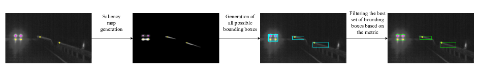
Figure 3: Bounding box generation pipeline using Boolean map saliency and the ground-truth keypoints. The first image shows the original scene with the light instances annotated via keypoints (pink: direct, yellow: indirect). In the first step, the saliency map for each keypoint is generated. For better visualization, the image shows the cumulated saliency map for all keypoints. Then, for each saliency map, the bounding boxes are determined. Finally, the combination of bounding boxes yielding the highest F-score and highest quality score is selected.

An example of these steps is shown in 3. We derive the optimal parameter setting for the saliency map generator by optimizing the product of the F-score and the quality $q$ on the whole PVDN dataset using a Tree-structured Parzen Estimator approach as it was also done by Ewecker et al. [45]. This can be considered as a standard hyperparameter tuning. Thus, saliency maps for the whole dataset are generated using the same parameter setting.

Table 1: Comparison of bounding box generation methods and performances of trained object detectors (mean $\pm$ standard deviation).

Model	Precision	Recall	F-score	$q$	$q_{K}$	$q_{B}$
Bounding Box Generation [2]	1.00	0.69	0.81	0.42	0.42$\thinspace\pm\thinspace$0.24	1.00$\thinspace\pm\thinspace$0.00
YoloV5s [2]	0.99	0.66	0.80	0.37	0.38$\thinspace\pm\thinspace$0.20	0.98$\thinspace\pm\thinspace$0.09
YoloV5x [2]	1.00	0.68	0.81	0.37	0.38$\thinspace\pm\thinspace$0.20	0.98$\thinspace\pm\thinspace$0.08
Bounding Box Generation [45]	1.00	0.87	0.93	0.70	0.70$\thinspace\pm\thinspace$0.30	1.00$\thinspace\pm\thinspace$0.00
YoloV5s [45]	0.98	0.67	0.80	0.67	0.70$\thinspace\pm\thinspace$0.31	0.97$\thinspace\pm\thinspace$0.12
YoloV5x [45]	0.99	0.76	0.86	0.67	0.69$\thinspace\pm\thinspace$0.30	0.98$\thinspace\pm\thinspace$0.10
Bounding Box Generation (ours)	0.99	0.93	0.96	0.86	0.86$\thinspace\pm\thinspace$0.25	1.00$\thinspace\pm\thinspace$0.00
YoloV5s (ours)	0.96	0.65	0.78	0.87	0.89$\thinspace\pm\thinspace$0.23	0.98$\thinspace\pm\thinspace$0.10
YoloV5x (ours)	0.97	0.58	0.73	0.86	0.87$\thinspace\pm\thinspace$0.24	1.00$\thinspace\pm\thinspace$0.04

The results of the proposed saliency-based bounding box generation approach are shown in 1. With our method for generating bounding boxes based on the keypoint annotations, we clearly outperform the previous approaches both in terms of F-score and bounding box quality [45, 2]. With a bounding box quality score of 0.86, we see that the bounding boxes, which are predicted correctly, are of very high quality. Specifically, the improvement of $q_{K}$ shows that a single bounding box often matches with exactly one keypoint, which indicates that small bounding boxes separate keypoints that are located close to each other. A high bounding box quality is desirable since it better reflects the original human annotations, meaning that for each annotated keypoint there exists in the optimal case exactly one unique derived bounding box.

4.2 SOTA Object Detector Evaluation

We trained the SOTA object detection algorithm YoloV5 on the newly generated bounding boxes using the small (YoloV5s) and large version (YoloV5x) to evaluate a run-time and detection performance optimized algorithm, respectively. We used the Adam optimizer with an initial learning rate of 0.01, weight decay of 0.0005, a batch size of 16 and 32 for YoloV5x and YoloV5s, respectively, trained for 200 epochs each, and evaluated on the official PVDN test dataset.

Training YoloV5 on our saliency-based bounding boxes produces competitive detection performance results compared to the benchmark by Saralajew et al. [2]. However, we achieve slightly lower detection performances than Ewecker et al. [45]. This is most likely caused by the fact that our ground-truth bounding boxes are often smaller and thus harder to detect than the ones created with the approach by Ewecker et al. [45]: They achieve a significantly lower bounding box quality, indicating that bounding boxes often span across several keypoints and, thus, are bigger than ours.

In terms of bounding box quality, we surpass the previous methods by Saralajew et al. [2] and Ewecker et al. [45]. YoloV5, as our SOTA object detection algorithm, is able to discriminate the different light instances much better when trained on our saliency-based bounding box annotations. By increasing the quality of the bounding boxes, the task inherently becomes more difficult since a high bounding box quality indicates that each keypoint has a single corresponding bounding box and only a few bounding boxes span over multiple keypoints. Thus, the algorithm has to distinguish between neighboring light instances and cannot simply predict a larger bounding box spanning over several keypoint annotations. This explanation provides a rationale for why YoloV5 performs slightly worse compared to Ewecker et al. [45] in terms of F-score, although being trained on better ground-truth bounding boxes. For future autonomous systems, it might be crucial to predict such high-quality bounding boxes, especially when several light instances in an image have to be associated with its sources (i. e., the vehicle that caused the light reflection). For that, it is crucial to distinguish precisely between different unique light instances and not mix them together as a single instance, which often happens with the previously published methods.

Looking at the quality measures, it becomes obvious that $q_{B}$ converges to 1.0 in all cases. Considering the definition of $q_{B}$ and the bounding box generation methods, this behavior is natural. The quality $q_{B}$ becomes 1.0 if each ground truth keypoint is covered by not more than one bounding box, meaning that bounding boxes do not overlap and multiple bounding boxes do not span over the same keypoint. For the bounding box generation algorithm proposed by Saralajew et al. [2] and Ewecker et al. [45] overlapping bounding boxes are mitigated by the non-maximum suppression at the end of the bounding box generation pipeline. In our saliency-based method, saliency maps that would normally overlap are merged together to a single box. When training YoloV5 variants on those bounding boxes, they filter out overlapping candidates by the final non-maximum suppression as well as learn to infer non-overlapping bounding boxes, therefore, also resulting in $q_{B}$ values that converge to 1.0.

5 Conclusion and Future Work

Following up on the previous work of Saralajew et al. [2], we presented an approach to generate various object representations based on sparse keypoint annotations using visual saliency in order to detect oncoming vehicles at night before they are actually directly visible. With our method, the fuzzy and unclear borders of light reflections can be properly modeled, thus, giving a more natural representation. We showed that when using our context-aware saliency approach, the task can easily be phrased as an object detection problem. The proposed approach is able to automatically generate high-quality bounding boxes based on the annotated keypoints describing the direct and indirect light instances. On the PVDN dataset, we set a new benchmark for automatically deriving bounding box annotations from human keypoint annotations. We also show that, when trained on our generated bounding boxes, the SOTA object detection algorithm YoloV5 is able to achieve superior results compared to previous works. This is especially important when building systems where it is necessary to find the correspondence between light artifacts and their emitting source, for example, when several vehicles are already visible, and it has to be determined to which vehicle a light artifact belongs. In this case, having precise and high-quality descriptions of the light artifacts is key.

In future work, we plan to use the saliency maps generated with our approach to develop algorithms that can directly handle the fuzzy boundaries of light reflections and that can deal with uncertain object borders. For that, our proposed saliency method builds the foundation by providing a framework to annotate objects with unclear boundaries.

In summary, in this paper, we provided further perspectives and tools that rely on visual saliency to tackle the problem of provident vehicle detection at night. At this point, we want to emphasize that although the methods are evaluated on the specific automotive use case, we are confident that they can be transferred to other domains where fuzzy and objectively non-definable object boundaries are present, such as biological image data of fluorescence microscopy.

References

- [1] E. Oldenziel, L. Ohnemus, and S. Saralajew, “Provident detection of vehicles at night,” in IEEE Intelligent Vehicles Symposium (IV), 2020, pp. 472–479.
- [2] S. Saralajew, L. Ohnemus, L. Ewecker, E. Asan, S. Isele, and S. Roos, “A dataset for provident vehicle detection at night,” in IEEE/RSJ International Conference on Intelligent Robots and Systems (IROS), 2021, pp. 9750–9757.
- [3] S. Chadwick and P. Newman, “Training object detectors with noisy data,” in IEEE Intelligent Vehicles Symposium (IV), 2019, pp. 1319–1325.
- [4] B. Frenay and M. Verleysen, “Classification in the presence of label noise: A survey,” IEEE Trans. Neural Networks Learn. Syst., vol. 25, no. 5, pp. 845–869, 2014.
- [5] J. Ma, Y. Ushiku, and M. Sagara, “The effect of improving annotation quality on object detection datasets: A preliminary study,” in IEEE/CVF Conference on Computer Vision and Pattern Recognition (CVPR) Workshops, 2022, pp. 4850–4859.
- [6] M. P. Schilling, T. Scherr, F. R. Münke, O. Neumann, M. Schutera, R. Mikut, and M. Reischl, “Automated annotator variability inspection for biomedical image segmentation,” IEEE Access, vol. 10, pp. 2753–2765, 2022.
- [7] J. Zhang and S. Sclaroff, “Saliency detection: A boolean map approach,” in IEEE International Conference on Computer Vision (ICCV), 2013, pp. 153–160.
- [8] I. Ullah, M. Jian, S. Hussain, J. Guo, H. Yu, X. Wang, and Y. Yin, “A brief survey of visual saliency detection,” Multim. Tools Appl., vol. 79, no. 45-46, pp. 34 605–34 645, 2020.
- [9] L. Itti, C. Koch, and E. Niebur, “A model of saliency-based visual attention for rapid scene analysis,” IEEE Transactions on Pattern Analysis and Machine Intelligence, vol. 20, no. 11, pp. 1254–1259, 1998.
- [10] L. Itti and C. Koch, “Comparison of feature combination strategies for saliency-based visual attention systems,” in Human Vision and Electronic Imaging IV, 1999, pp. 473–482.
- [11] M. Jian, W. Zhang, H. Yu, C. Cui, X. Nie, H. Zhang, and Y. Yin, “Saliency detection based on directional patches extraction and principal local color contrast,” J. Vis. Commun. Image Represent., vol. 57, pp. 1–11, 2018.
- [12] J. Zhang, Y. Dai, and F. Porikli, “Deep salient object detection by integrating multi-level cues,” in IEEE Winter Conference on Applications of Computer Vision (WACV), 2017, pp. 1–10.
- [13] J. Pan, E. Sayrol, X. Giro-i Nieto, K. McGuinness, and N. E. O’Connor, “Shallow and deep convolutional networks for saliency prediction,” in IEEE Conference on Computer Vision and Pattern Recognition (CVPR), 2016, pp. 598–606.
- [14] A. Kroner, M. Senden, K. Driessens, and R. Goebel, “Contextual encoder-decoder network for visual saliency prediction,” Neural Networks, vol. 129, pp. 261–270, 2020.
- [15] N. Liu, N. Zhang, K. Wan, L. Shao, and J. Han, “Visual saliency transformer,” in IEEE/CVF International Conference on Computer Vision (ICCV), 2021, pp. 4702–4712.
- [16] G. Li, Y. Xie, L. Lin, and Y. Yu, “Instance-level salient object segmentation,” in IEEE Conference on Computer Vision and Pattern Recognition (CVPR), 2017, pp. 247–256.
- [17] A. Borji and L. Itti, “CAT2000: A large scale fixation dataset for boosting saliency research,” arXiv preprint arXiv:1505.03581, 2015.
- [18] M. Andriluka, L. Pishchulin, P. Gehler, and B. Schiele, “2D human pose estimation: New benchmark and state of the art analysis,” in IEEE Conference on Computer Vision and Pattern Recognition (CVPR), 2014, pp. 3686–3693.
- [19] V. Belagiannis and A. Zisserman, “Recurrent human pose estimation,” in IEEE International Conference on Automatic Face & Gesture Recognition (FG), 2017, pp. 468–475.
- [20] J. Carreira, P. Agrawal, K. Fragkiadaki, and J. Malik, “Human pose estimation with iterative error feedback,” in IEEE Conference on Computer Vision and Pattern Recognition (CVPR), 2016, pp. 4733–4742.
- [21] J. Maldonado and L. A. Giefer, “A comparison of bottom-up models for spatial saliency predictions in autonomous driving,” Sensors, vol. 21, no. 20, pp. 1–18, 2021.
- [22] F. Lateef, M. Kas, and Y. Ruichek, “Saliency heat-map as visual attention for autonomous driving using generative adversarial network (GAN),” IEEE Trans. Intell. Transp. Syst., vol. 23, no. 6, pp. 5360–5373, 2021.
- [23] N. Pugeault and R. Bowden, “How much of driving is preattentive?” IEEE Trans. Veh. Technol., vol. 64, no. 12, pp. 5424–5438, 2015.
- [24] A. López, J. Hilgenstock, A. Busse, R. Baldrich, F. Lumbreras, and J. Serrat, “Nighttime vehicle detection for intelligent headlight control,” in Advanced Concepts for Intelligent Vision Systems, 2008, pp. 113–124.
- [25] P. Alcantarilla, L. Bergasa, P. Jiménez, I. Parra, D. Fernández, M.A. Sotelo, and S.S. Mayoral, “Automatic LightBeam controller for driver assistance,” Mach. Vis. Appl., vol. 22, no. 5, pp. 819–835, 2011.
- [26] S. Eum and H. G. Jung, “Enhancing light blob detection for intelligent headlight control using lane detection,” IEEE Trans. Intell. Transp. Syst., vol. 14, no. 2, pp. 1003–1011, 2013.
- [27] D. Jurić and S. Lončarić, “A method for on-road night-time vehicle headlight detection and tracking,” in International Conference on Connected Vehicles and Expo (ICCVE), 2014, pp. 655–660.
- [28] P. Sevekar and S. B. Dhonde, “Nighttime vehicle detection for intelligent headlight control: A review,” in International Conference on Applied and Theoretical Computing and Communication Technology (iCATccT), 2016, pp. 188–190.
- [29] R. K. Satzoda and M. M. Trivedi, “Looking at vehicles in the night: Detection and dynamics of rear lights,” IEEE Trans. Intell. Transp. Syst., vol. 20, no. 12, pp. 4297–4307, 2019.
- [30] L. Ewecker, E. Asan, and S. Roos, “Detecting vehicles in the dark in urban environments-a human benchmark,” in IEEE Intelligent Vehicles Symposium (IV), 2022, pp. 1145–1151.
- [31] H. Caesar, V. Bankiti, A. H. Lang, S. Vora, V. E. Liong, Q. Xu, A. Krishnan, Y. Pan, G. Baldan, and O. Beijbom, “nuScenes: A multimodal dataset for autonomous driving,” in IEEE/CVF Conference on Computer Vision and Pattern Recognition (CVPR), 2020, pp. 11 618–11 628.
- [32] A. Geiger, P. Lenz, and R. Urtasun, “Are we ready for autonomous driving? The KITTI vision benchmark suite,” in IEEE Conference on Computer Vision and Pattern Recognition (CVPR), 2012, pp. 3354–3361.
- [33] T.-Y. Lin, M. Maire, S. Belongie, J. Hays, P. Perona, D. Ramanan, P. Dollár, and C. L. Zitnick, “Microsoft COCO: Common objects in context,” in European Conference on Computer Vision (ECCV), 2014, pp. 740–755.
- [34] F. Yu, H. Chen, X. Wang, W. Xian, Y. Chen, F. Liu, V. Madhavan, and T. Darrell, “Bdd100k: A diverse driving dataset for heterogeneous multitask learning,” in IEEE/CVF Conference on Computer Vision and Pattern Recognition (CVPR), 2020, pp. 2633–2642.
- [35] N. C. F. Codella, D. A. Gutman, M. E. Celebi, B. Helba, M. A. Marchetti, S. W. Dusza, A. Kalloo, K. Liopyris, N. K. Mishra, H. Kittler, and A. Halpern, “Skin lesion analysis toward melanoma detection: A challenge at the 2017 international symposium on biomedical imaging (isbi), hosted by the international skin imaging collaboration (ISIC),” in IEEE International Symposium on Biomedical Imaging (ISBI), 2018, pp. 168–172.
- [36] R. S. Lee, F. Gimenez, A. Hoogi, K. K. Miyake, M. Gorovoy, and D. L. Rubin, “A curated mammography data set for use in computer-aided detection and diagnosis research,” Scientific Data, vol. 4, no. 1, pp. 1–9, 2017.
- [37] I. Smal, M. Loog, W. Niessen, and E. Meijering, “Quantitative comparison of spot detection methods in fluorescence microscopy,” IEEE Trans. Medical Imaging, vol. 29, no. 2, pp. 282–301, 2010.
- [38] A. C.-Y. Wu and S. A. Rifkin, “Aro: A machine learning approach to identifying single molecules and estimating classification error in fluorescence microscopy images,” BMC Bioinform., vol. 16, pp. 1–8, 2015.
- [39] S. Abousamra, S. Adar, N. Elia, and R. Shilkrot, “Localization and tracking in 4D fluorescence microscopy imagery,” in IEEE Conference on Computer Vision and Pattern Recognition (CVPR) Workshops, 2018, pp. 2290–2298.
- [40] M. McKenna, S. Wang, T. B. Nguyen, J. E. Burns, N. Petrick, and R. M. Summers, “Strategies for improved interpretation of computer-aided detections for CT colonography utilizing distributed human intelligence,” Medical Image Anal., vol. 16, no. 6, pp. 1280–1292, 2012.
- [41] T. B. Nguyen, S. Wang, V. Anugu, N. Rose, M. McKenna, N. Petrick, J. E. Burns, and R. M. Summers, “Distributed human intelligence for colonic polyp classification in computer-aided detection for CT colonography,” Radiology, vol. 262, no. 3, pp. 824–833, 2012.
- [42] S. Albarqouni, C. Baur, F. Achilles, V. Belagiannis, S. Demirci, and N. Navab, “AggNet: Deep learning from crowds for mitosis detection in breast cancer histology images,” IEEE Trans. Medical Imaging, vol. 35, no. 5, pp. 1313–1321, 2016.
- [43] J. Zhang and S. Sclaroff, “Exploiting surroundedness for saliency detection: A Boolean map approach,” IEEE Trans. Pattern Anal. Mach. Intell., vol. 38, no. 5, pp. 889–902, 2015.
- [44] L. Liu, W. Ouyang, X. Wang, P. Fieguth, J. Chen, X. Liu, and M. Pietikäinen, “Deep learning for generic object detection: A survey,” Int. J. Comput. Vis., vol. 128, no. 2, pp. 261–318, 2019.
- [45] L. Ewecker, E. Asan, L. Ohnemus, and S. Saralajew, “Provident vehicle detection at night for advanced driver assistance systems,” arXiv preprint arXiv:2107.11302, 2021.