Surpassing the Human Accuracy:
Detecting Gallbladder Cancer from USG Images with Curriculum Learning

Abstract

We explore the potential of cnn-based models for gallbladder cancer (gbc) detection from ultrasound (usg) images. usg is the most common diagnostic modality for gb diseases due to its low cost and accessibility. However, usg images are challenging to analyze due to low image quality because of noise and varying viewpoints due to the handheld nature of the sensor. Our exhaustive study of state-of-the-art (sota) image classification techniques for the problem reveals that they often fail to learn the salient gb region due to the presence of shadows in the usg images. sota object detection techniques also achieve low accuracy because of spurious textures due to noise or adjacent organs. We propose GBCNet to tackle the challenges in our problem. GBCNet first extracts the regions of interest (rois) by detecting the gb (and not the cancer), and then uses a new multi-scale, second-order pooling architecture specializing in classifying gbc. To effectively handle spurious textures, we propose a curriculum inspired by human visual acuity, which reduces the texture biases in GBCNet. Experimental results demonstrate that GBCNet significantly outperforms sota cnn models, as well as the expert radiologists. Our technical innovations are generic to other usg image analysis tasks as well. Hence, as a validation, we also show the efficacy of GBCNet in detecting breast cancer from usg images. Project page with source code, trained models, and data is available at https://gbc-iitd.github.io/gbcnet.

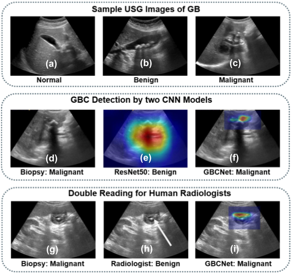
Figure 1: (a), (b), and (c) Normal, benign, and malignant gb sample in usg images, respectively. While normal or benign gb have regular anatomy, clear boundary is absent in malignant gb. (d) A malignant (biopsy-proven) gb sample. (e) Shadows having visual traits of a gb leads to localization error in ResNet50. (f) gbcnet tackles shadow artifacts well. (g) Another sample of malignant gb. (h) The radiologist incorrectly diagnosed the gb as benign based on the stone and wall thickening. (i) gbcnet helps the radiologist to identify the salient region with liver infiltration by the gb, a critical feature of gbc, and correct the prediction.

1 Introduction

According to GLOBOCAN 2018 [10], worldwide about 165,000 people die of gbc annually. For most patients, gbc is detected at an advanced stage, with a mean survival rate for patients with advanced gbc of six months and a 5-year survival rate of 5% [41, 28]. Detecting gbc at an early stage could ameliorate the bleak survival rate.

Lately, machine learning models based on convolutional neural network (cnn) architectures have made transformational progress in radiology, and medical diagnosis for diseases such as breast cancer, lung cancer, pancreatic cancer, and melanoma [3, 5, 16, 17, 29]. However, their usage is conspicuously absent for the gbc detection. Although there has been prior work involving segmentation and detection of the gb abnormalities such as stones and polyps [14, 31, 35], detection of gbc is missing from the list. A search on Google Scholar with keywords “artificial intelligence” and “gallbladder cancer” returned 204 articles between 2015-2021 (November). In these, we did not find any published article on deep learning-based gbc detection from usg images.

Early diagnosis and resection are critical for improving the survival rate of gbc. Due to the non-ionizing radiation, low cost, portability, and accessibility, usg is a popular diagnostic imaging modality. Although identifying anomalies such as stones or gb wall thickening at routine usg is easy, accurate characterization is challenging [27, 25]. Often, usg is the sole diagnostic imaging performed for patients with suspected gb ailments. If malignancy is not suspected, no further testing is usually performed, and gbc could silently advance. Therefore, it is imperative to develop and understand the characterization of gb malignancy from usg images.

There are significant challenges in using cnn models for usg image analysis. Unlike mri or ct, usg images suffer from low imaging quality due to noise and other sensor artifacts. The views are also not aligned due to the handheld nature of the sensor. We observe that modern cnn classifiers fail to localize the salient gb region due to the presence of shadows which often have similar visual traits of a gb in usg images (Fig. 1). Training object detectors for gbc detection gets biased towards learning from spurious textures due to noise and adjacent organ tissues rather than the shape or boundary of gb wall, which results in poor accuracy. Further, unlike normal and benign gb regions, which have regular anatomy, malignant cases are much harder to detect due to the absence of a clear gb boundary or shape and the presence of a mass.

Contributions: The key contributions of this work are:

1. We focus on circumventing the challenges for automated detection of gbc from usg images and propose a deep neural network, GBCNet, for detecting gbc from usg images. GBCNet extracts candidate regions of interest (rois) from the usg to mitigate the effects of shadows and then uses a new multi-scale, second-order pooling-based (MS-SoP) classifier on the rois to classify gallbladder malignancy. MS-SoP encodes rich feature representations for malignancy detection.

2. Even though GBCNet shows improvement in gb malignancy detection over multiple sota models, the spurious texture present in an roi bias the classification unit towards generating false positives. To alleviate the issue, we propose a training curriculum inspired by human visual acuity [33, 54]. Visual acuity refers to the sharpness of visual stimuli. The proposed curriculum mitigates texture bias and helps GBCNet focus on shape features important for accurate gbc detection from usg images.

3. A lack of publicly available usg image datasets related to gb malignancy adds to the difficulty of utilizing cnn models for detecting gbc. We have collected, annotated, and curated a usg image dataset of 1255 abdominal usg images collected from 218 patients. We refer this dataset as the Gallbladder Cancer Ultrasound (GBCU) dataset.

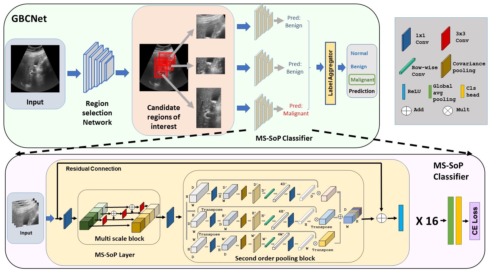
Figure 2: Overview of the gbcnet architecture. The region selection network localizes the candidate regions of interest and the multi-scale, second-order pooling-based (MS-SoP) classifier at the next stage predicts malignancy for each region. The predictions for each region is aggregated to get the final prediction on the whole image.

2 Related Work

Deep Learning for GB Abnormalities: usg imaging is an effective modality for diagnosing gbc and related gb afflictions [59]. Lien et. al[35] use a parameter-adaptive pulse-coupled neural network for gb stone segmentation in usg images. Pang et. al[40] identify gb and gallstones using a YOLOv3 model from ct images. Jeong et. al[31] uses an InceptionV3 model to classify neoplastic polyps from cropped samples of gb usg images. gbc is a serious problem affecting a significant number of people. Despite the presence of numerous studies on using deep learning on other gb-related afflictions, there is an absence of any work that applies deep learning for gbc detection on usg images.

Deep Learning for USG: cnn models have been widely applied in usg imaging tasks, such as ovarian cancer detection [60], breast cancer region, mass and boundary detection [7, 13, 58, 38, 61], measuring head circumference in fetal usg images [50, 12].

Curriculum Learning: Curriculum learning has been applied to different medical imaging tasks. While Jesson et. al[32] used a patch-based curriculum for lung nodule detection, Tang et. al[53] used disease severity level to identify thoracic diseases from chest radiographs. Oksuz et. al[39] proposed image corruption-based curriculum to detect motion artifacts in cardiac mri.

Texture Bias in Neural Networks: Presence of mass and a thickened gb wall are prominent indicators of gb abnormality. However, typical cnn-based architectures are biased towards textures rather than shape [24]. This may lead GBCNet to focus on soft tissue textures such as liver rather than noticing cues based on the shape and wall of the gb. Multiple works have attempted to reduce texture bias and improve the spatial understanding of a model. Geirhos et. al[24] suggest style transfer to replace the original texture of images while Brendel et. al[11] propose a method similar to a Bag of Features model to force spatial learning.

Visual Acuity in Learning Models: Vogelsang et. al[54] suggest that a period of low visual acuity (blurred vision) followed by high visual acuity induces better spatial processing and also increases the receptive field in human vision. Different from our visual acuity-inspired strategy of working with input space, Sinha et. al[47] propose applying a Gaussian kernel on the output feature map of every layer of a network. The use of blurring before pooling seems to mitigate aliasing effects due to sub-sampling in the pooling layer rather than the use of visual acuity. Azad et. al[4] have integrated a Difference of Gaussian (DoG) operation into their model. Similar to [47], they end up attenuating the high frequency in the feature maps corresponding to every layer rather than the input image, for which there is no obvious biological connection known. On the other hand, our proposed visual acuity-based curriculum works in the input space and has a solid neural basis [54].

3 Proposed Method

3.1 Model Architecture

The artifacts in usg images often result in multiple spurious areas in a usg image with very similar visual traits as the gb region, leading to a disappointing performance by the baseline classifiers. GBCNet selects candidate regions of interest (rois) from the usg to mitigate the influence of spurious artifacts like shadows and then uses a multi-scale, second-order pooling-based (MS-SoP) classifier on the rois. Fig. 2 presents a conceptual diagram of the architecture. At test time, the detector may predict multiple rois overlapping with the gb. Occasionally, the detection network may fail to localize the rois. In this case, we pass the entire image to the classifier. The proposed MS-SoP classifier exploits a range of spatial scales and second-order statistics to generate rich features from usg images to learn the characteristics of malignancy. We run the classifier for each candidate region during inference and aggregate the predicted labels to compute the prediction for the entire image. If any of the rois is classified as malignant, the image as the whole is classified as malignant. If all the regions are predicted to be normal, the image is classified as normal. In all other cases, the image is predicted to be benign.

Candidate roi Selection: We used deep object detection networks to localize the gb region in a usg image. The predicted bounding boxes serve as candidate regions of interest and mitigate the adverse effect of noise and artifacts from non-gb regions during the classification. For training the roi selection models, we use only two classes - background and the gb region. In this stage, we only detect the gb and do not classify them as malignant or non-malignant. In principle, it is possible to do both in a single stage, but we observed that using a separate classifier on the focused rois leads to better accuracy. We note that our findings regarding the superiority of using classification on focused regions, instead of over the entire image, are consistent with other recent works [48, 13, 6, 21, 55]. Prior studies demonstrate that modern object detection architectures such as YOLO [9] or Faster-RCNN [42] can detect breast lesions in usg images [13]. On the other hand, recently proposed anchor-free approaches, such as Reppoints [57], and CentripetalNet [20] can detect unconventionally sized objects such as gb. Hence, we experimented with all the above approaches for roi selection in our framework.

MS-SoP Classifier: Modeling higher-order statistics has gained popularity in recent years due to its enhanced ability to capture complex features and non-linearity in deep neural networks [62, 34, 23]. Ning et. al[38] recently used higher-order feature fusion for classifying breast lesions. They have used RGB image patches of three fixed scales at the input layer. We take the idea further and develop a novel multi-scale, second-order pooling (MS-SoP) layer to encode rich features suitable for malignant gb detection. In contrast to [38], we exploit feature maps of multiple scales in all the intermediate layers to learn a rich representation. The proposed MS-SoP layers can be conveniently plugged into any cnn backbone. The MS-SoP classifier contains $16$ MS-SoP layers as the backbone, followed by global average pooling and a fully connected classification head. We use the Categorical Cross-Entropy loss to train the classifier.

Multi-Scale Block: Abdominal organs can appear in significantly different sizes in a usg image based on the insonation angle or the pressure on the transducer. Perceiving information across multiple scales is thus necessary for accurate gbc detection. Recently, Gao et. al[22] have replaced the standard convolution block in the bottleneck layer with group convolution to add a multi-scale capability to the ResNet architecture. Inspired by [22], we used a hierarchy of convolution kernels on slices of feature volumes in the intermediate layers to capture multi-scale information through a combination of different receptive fields. We split a feature map volume, $\mathcal{X}\!\in\!\mathbb{R}^{H\!\times\!W\!\times\!D}$ ($H,W~{}\text{and}~{}D$ are the height, width, and the number of channels, respectively), depth-wise into 4 slices, $\mathcal{X}_{1},\mathcal{X}_{2},\mathcal{X}_{3}$, and $\mathcal{X}_{4}$, where $\mathcal{X}_{i}\!\in\!\mathbb{R}^{H\!\times\!W\!\times\!D/4}$. Each $\mathcal{X}_{i}$ will generate an output split $\mathcal{Y}_{i}$. The final output, $\mathcal{Y}$, is obtained by concatenating the splits. Suppose $\mathcal{C}_{j}$ are $3\!\times\!3$ convolution kernels and $\stackMath\mathbin{\stackinset{c}{0ex}{c}{0ex}{\ast}{\bigcirc}}$ denotes the convolution. We get each $\mathcal{Y}_{i}$ as follows: $\displaystyle\mathcal{Y}_{1}$ $\displaystyle=\mathcal{X}_{1}$ (1) $\displaystyle\mathcal{Y}_{2}$ $\displaystyle=\mathcal{C}_{1}\stackMath\mathbin{\stackinset{c}{0ex}{c}{0ex}{\ast}{\bigcirc}}\mathcal{X}_{2}$ (2) $\displaystyle\mathcal{Y}_{3}$ $\displaystyle=\mathcal{C}_{2}\stackMath\mathbin{\stackinset{c}{0ex}{c}{0ex}{\ast}{\bigcirc}}(\mathcal{X}_{3}\!+\!\mathcal{Y}_{2})$ (3) $\displaystyle\mathcal{Y}_{4}$ $\displaystyle=\mathcal{C}_{3}\stackMath\mathbin{\stackinset{c}{0ex}{c}{0ex}{\ast}{\bigcirc}}(\mathcal{X}_{4}\!+\!\mathcal{Y}_{3})$ (4)

Second-order Pooling Block: Traditional average or max-pooling use first-order statistics and thus cannot capture the higher-order statistical relation between features. Inspired by the recent success of higher-order statistics in breast lesion usg [38, 61], we employ the second-order pooling (SoP) mechanism to exploit the second-order statistical dependency between the multi-scale features.

For computational efficiency, we reduce the number of channels of a feature volume, $\mathcal{X}\!\in\!\mathbb{R}^{H\!\times\!W\!\times\!D}$, to $D^{\prime}~{}(D^{\prime}\!<\!D)$, using $1\!\times\!1$ convolutions. $\mathcal{X}$ is then reshaped to a matrix $\mathbf{X}\!\in\!\mathbb{R}^{D^{\prime}\!\times\!N}$, where $N\!=\!H\!\times\!W$. We compute the covariance of $\mathbf{X}$ as, $\mathbf{C}_{D^{\prime}\!\times\!D^{\prime}}\!=\!(\mathbf{X\!-\!\bar{X}})\mathbf{(X\!-\!\bar{X})^{T}}$, which is then reshaped to a tensor of size $1\!\times\!D^{\prime}\!\times\!D^{\prime}$ and passed through a convolution layer with $4D^{\prime}$ kernels of size $1\!\times\!D^{\prime}$ each. We resize the resulting $1\!\times\!1\!\times\!4D^{\prime}$ tensor to a $1\!\times\!1\!\times\!D$ tensor, $\mathbf{w_{d}}$, by $1\!\times\!1$ convolutions. $\mathbf{w_{d}}$ represents the weight for each channel. These weights are then channel-wise multiplied with $\mathcal{X}$, to obtain the weighted feature map $\mathbf{Z_{d}}$. To repeat similar processes for the height and width, we transpose $\mathcal{X}$ from to a $D\!\times\!W\!\times\!H$ tensor, say $\mathcal{X}_{h}$ and to a $H\!\times\!D\!\times\!W$ tensor, say $\mathcal{X}_{w}$. In terms of index notation, $\mathcal{X}_{h}[k,j,i]\!=\!\mathcal{X}[i,j,k]$ and $\mathcal{X}_{w}[i,k,j]\!=\!\mathcal{X}[i,j,k]$, where $i\!=\!\{1,2,\ldots H\},~{}j\!=\!\{1,2,\ldots W\},$ and $k\!=\!\{1,2,\ldots D\}$. Similar to calculating $\mathbf{w_{h}}$ from $\mathcal{X}$, we find $\mathbf{w_{h}}\!\in\!\mathbb{R}^{1\!\times\!1\!\times\!H}$ from $\mathcal{X}_{h}$, and $\mathbf{w_{w}}\!\in\!\mathbb{R}^{1\!\times\!1\!\times\!W}$ from $\mathcal{X}_{w}$. We also calculate $\mathbf{Z_{h}}$ and $\mathbf{Z_{w}}$ by multiplying $\mathbf{w_{h}}$ and $\mathbf{w_{w}}$ channel-wise to $\mathcal{X}_{h}$ and $\mathcal{X}_{w}$. Then, we transpose $\mathbf{Z_{h}}$ and $\mathbf{Z_{w}}$ to tensors of size $H\!\times\!W\!\times\!D$, say $\mathbf{Z_{h}}^{T}$ and $\mathbf{Z_{w}}^{T}$, respectively, where $\mathbf{Z_{h}}^{T}[i,j,k]=\mathbf{Z_{h}}[k,j,i]$ and $\mathbf{Z_{w}}^{T}[i,j,k]=\mathbf{Z_{w}}[i,k,j]$. Finally, we obtain the output feature tensor, $\mathbf{Z}\!\in\!\mathbb{R}^{H\!\times\!W\!\times\!D}$ by adding $\mathbf{Z_{d}},\mathbf{Z_{h}}^{T},$ and $\mathbf{Z_{w}}^{T}$.

$$\mathbf{Z_{d}}[i,j,k] =\mathbf{w_{d}}[k]~{}~{}\mathcal{X}[i,j,k]$$ (5)

$$\mathbf{Z_{h}}[k,j,i] =\mathbf{w_{h}}[i]~{}~{}\mathcal{X}_{h}[k,j,i]$$ (6)

$$\mathbf{Z_{w}}[i,k,j] =\mathbf{w_{w}}[j]~{}~{}\mathcal{X}_{w}[i,k,j]$$ (7)

$$\mathbf{Z}[i,j,k] =\mathbf{Z_{d}}[i,j,k]+\mathbf{Z_{h}}^{T}[i,j,k]+\mathbf{Z_{w}}^{T}[i,j,k]$$ (8)

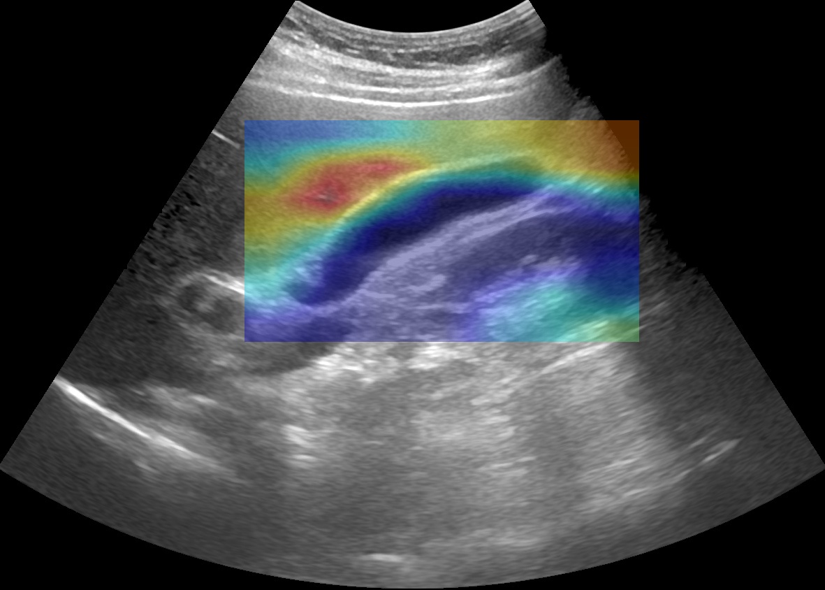
(a)

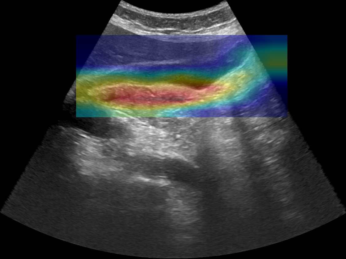
(b)

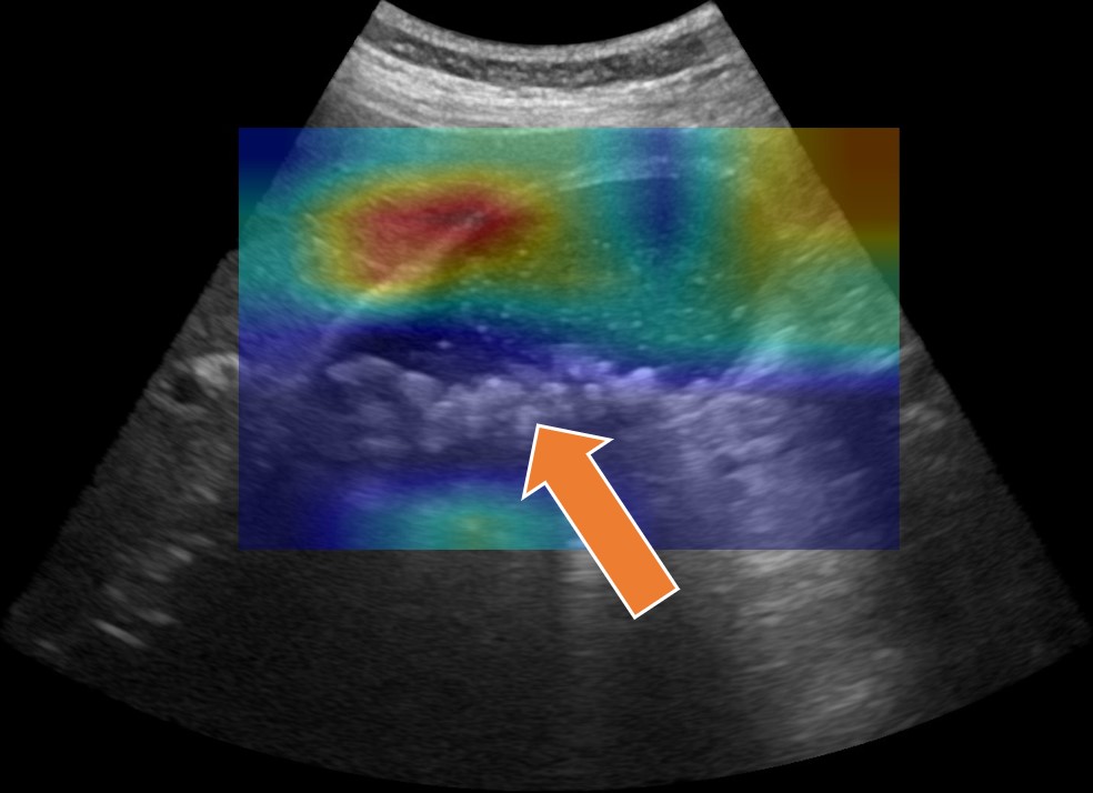
(c)

Figure 3: Grad-CAM visual of GBCNet trained without curriculum showing how the model tends to get biased due to the presence of textures due to noise or organ tissue. GBCNet focuses on - (a) adjacent liver tissues than the normal gb, (b) the echogenic region below the gb, and (c) liver textures instead of the stones (highlighted using the arrow).

3.2 Visual Acuity Inspired Curriculum

We found that the textures having visual characteristics of soft tissue can adversely affect the performance of GBCNet (Fig. 3). We propose a curriculum to mitigate the texture bias and improve the classification. We observed that while the MS-SoP classifier is affected by texture bias, the region selection network still maintains a very high recall (Tab. 2). Hence, we used the curriculum training only on the classifier and not on the region selection network.

Visual Acuity in Humans: Visual Acuity (VA) refers to the clarity and sharpness of human vision. Due to the immaturity of the retina and visual cortex, newborn children have very low VA [18]. The VA improves with the maturation of the retina and visual cortex. However, for children with congenital cataracts, the cortex matures despite the lenticular opacity. Such children begin their visual activity with higher initial VA. Evidence shows that children with high initial VA suffer to facilitate spatial analysis over expansive areas [54]. Low VA renders blurry images that do not contain enough local information for the visual cortex to identify patterns. As a result, the visual cortex tries to increase the receptive field to facilitate spatial analysis over expansive areas and learn global features [33, 49].

Gaussian Blurring to Simulate Visual Acuity: Gaussian filters are low-pass filters to cloak the high-frequency components of an input. A standard deviation $\sigma$ parameterizes the Gaussian filters. Increasing the $\sigma$ generates a higher amount of blur and low VA when convolved with an image. Fig. 4 shows how we can decrease the VA by increasing the $\sigma$ of a Gaussian filter. In our experiments, we have varied $\sigma$ from $1$ to $16$ to generate different levels of VA.

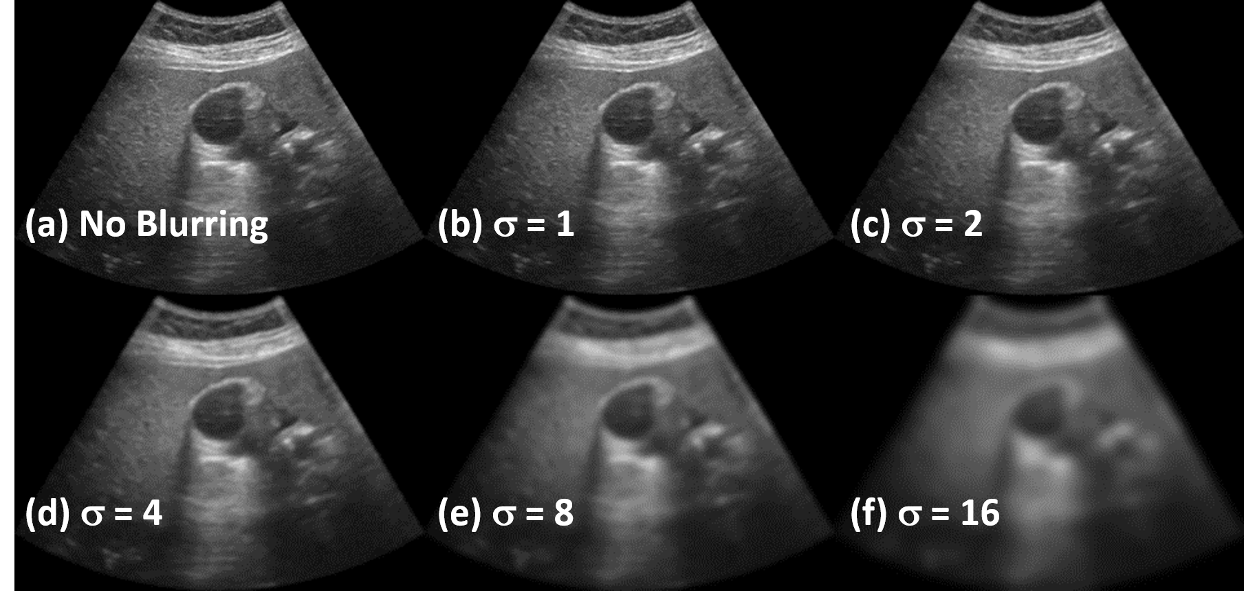
Figure 4: We simulate visual acuity through the Gaussian blur. Increasing $\sigma$ in a Gaussian filter decreases the visual acuity. Notice in the figure that, the effect of textures reduce as the visual acuity decreases and gb shape and structure become more pronounced.

Proposed Curriculum: While [54] demonstrates the improvement in receptive fields by gradually improving the sharpness of images during training, we take this observation further and show that the strategy of training on progressively higher resolution images also reduces the texture bias of a classification model. We propose a visual acuity-based training curriculum (Algorithm 1) that starts training the network with blurry and low-resolution usg images and progressively increase the sharpness of training samples. The initial blurring allows the model to use an extended receptive field and focus on learning the global features such as the shape of the gb while ignoring any noise or irrelevant textures. In the later phases, the sharp images allow the model to focus on the relevant local features in a controlled manner to make more accurate predictions.

Input: $D^{\text{train}}$, Dataset of regions cropped from the original USG images.

Output: Optimized model parameters $W^{*}$

Initialize $\sigma=\sigma_{0}$ ;

Initialize model parameters to $W$ ;

for epoch=$\{1\ldots,N\}$ do

       if $\sigma>0$ then

             $Z=\phi$ ;

             for $x\in D^{\text{train}}$ do

                   $Z=Z\cup\{x\stackMath\mathbin{\stackinset{c}{0ex}{c}{0ex}{\ast}{\bigcirc}}G(\sigma)\}$ ;

                  

             end for

            train($W,Z$);

            

      else

             train($W,D^{\text{train}}$) ;

            

       end if

      if (epoch $>k^{\prime}$) and (epoch$\%k==0$) then

             $\sigma=\lfloor\sigma/2\rfloor$ ;

            

       end if

      

end for

Algorithm 1 Proposed VA-based curriculum

4 Dataset Collection and Curation

Data Collection: We acquired data samples from patients referred to PGIMER, Chandigarh (a tertiary care referral hospital in Northern India) for abdominal ultrasound examinations of suspected gb pathologies. The study was approved by the Ethics Committee of PGIMER. We obtained informed written consent from the patients at the time of recruitment, and protect their privacy by fully anonymizing the data. Minimum 10 grayscale B-mode static images, including both sagittal and axial sections, were recorded by radiologists for each patient using a Logiq S8 machine. We excluded color Doppler, spectral Doppler, annotations, and measurements. Supplementary A contains more details of the data acquisition process.

Labeling and ROI Annotation: Each image is labeled as one of the three classes - normal, benign, or malignant. The ground-truth labels were biopsy-proven to assert the correctness. Additionally, in each image, expert radiologists have drawn an axis-aligned bounding box spanning the entire gb and adjacent liver parenchyma to annotate the roi.

Dataset Statistics: We have annotated 1255 abdominal usg images collected from 218 patients from the acquired image corpus. Overall, we have 432 normal, 558 benign, and 265 malignant images. Of the 218 patients, 71, 100, and 47 were from the normal, benign, and malignant classes, respectively. The width of the images was between 801 and 1556 pixels, and the height was between 564 and 947 pixels due to the cropping of patient-related information.

Dataset Splits: The sizes of the training and testing sets are 1133 and 122, respectively. To ensure generalization to unseen patients, all images of any particular patient were either in the train or the test split. The number of normal, benign, and malignant samples in the train and test set is 401, 509, 223, and 31, 49, and 42, respectively. Additionally, we report the 10-fold cross-validation metrics on the entire dataset for key experiments to assess generalization. All images of any particular patient appeared either in the training or the validation split during the cross-validation.

Method	Test Set				Cross Val.
	Acc.	Acc.-2	Spec.	Sens.	Acc.	Spec.	Sens.
Radiologist A	70.0	81.6	87.3	70.7	–	–	–
Radiologist B	68.3	78.4	81.1	73.2	–	–	–
VGG16	62.3	72.1	90.0	38.1	69.3 $\pm$ 3.6	96.0 $\pm$ 4.6	49.5 $\pm$ 23.4
ResNet50	76.2	78.7	87.5	61.9	81.1 $\pm$ 3.1	92.6 $\pm$ 6.9	67.2 $\pm$ 14.7
InceptionV3	77.9	85.0	87.5	80.1	84.4 $\pm$ 3.9	95.3 $\pm$ 2.9	80.7 $\pm$   9.7
Faster-RCNN	71.3	77.9	76.2	81.0	75.7 $\pm$ 5.3	84.0 $\pm$ 4.6	80.8 $\pm$ 10.4
RetinaNet	75.4	83.6	86.3	78.6	74.9 $\pm$ 7.3	86.7 $\pm$ 7.8	79.1 $\pm$   8.9
EfficientDet	58.2	77.9	86.3	62.0	73.9 $\pm$ 8.4	88.1 $\pm$ 9.9	85.8 $\pm$   6.1
GBCNet	87.7	91.0	90.0	92.9	88.2 $\pm$ 5.1	94.2 $\pm$ 3.7	92.3 $\pm$   7.1
GBCNet+VA	91.0	95.9	95.0	97.6	92.1 $\pm$ 2.9	96.7 $\pm$ 2.3	91.9 $\pm$   6.3

Table 1: The model performances on the test set and the 10-fold cross validation (Mean$\pm$SD) in classifying gbc from USG images. Apart from the standard accuracy of classifying normal, benign, and malignant gb, we show the binary classification (malignancy vs. non-malignancy) accuracy on the test set (column Acc.-2). We also report the gbc detection performance of two expert radiologists on the test set. The radiologists classified each test image without accessing the biopsy results or any other patient data. Note that our model significantly outperforms even the human radiologists. Recall that our ground truth labels are biopsy-proven. The performance of human radiologists in the our study is comparable to that reported in literature [8, 26].

5 Implementation and Evaluation

Transfer Learning and Data Augmentation: Studies show that pre-training on natural image data improves network performance on medical image data [2, 15]. We use roi detection networks pre-trained on the COCO [37], and classifiers pre-trained on ImageNet data [19]. We use resizing, center-cropping, and normalization data augmentations to avoid over-fitting on the small usg dataset.

Hyper-parameters: Details of the hyper-parameters are in the supplementary C. We train and freeze the roi detection network before training the classifier. We used $\sigma_{0}\!=\!16$, $k^{\prime}\!=\!10$, $k\!=\!5$, for the curriculum.

Evaluation metrics: We use mean intersection over union (mIoU), precision, and recall for comparing region selection models. We compute the precision and recall as suggested by [43] (details in the supplementary D). To assess the classification models for gbc detection, we use accuracy, sensitivity, and specificity as the evaluation metrics.

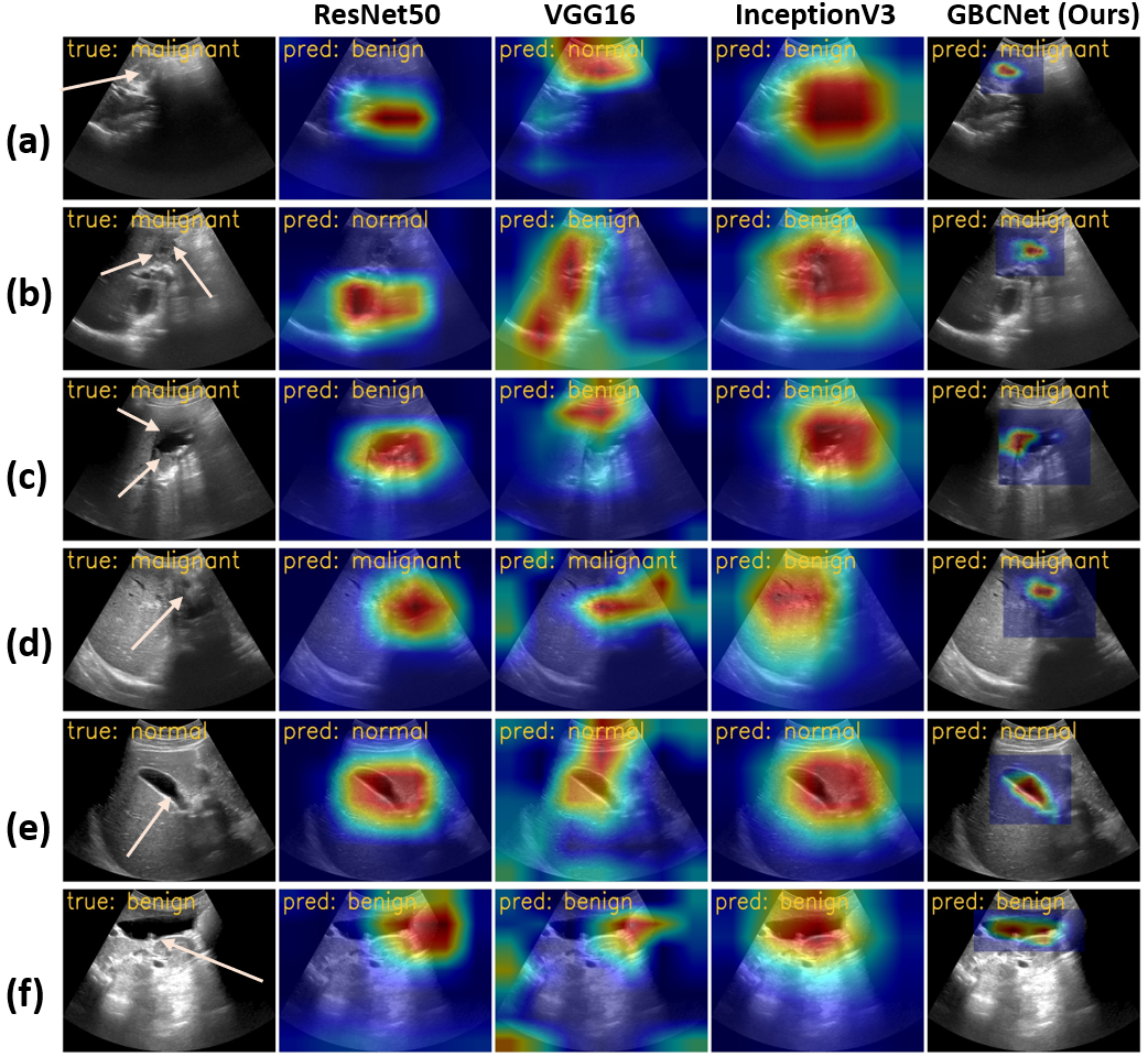
Figure 5: Grad-CAM visuals and the predictions for ResNet50, VGG16, Inception-V3, and GBCNet. The pathological areas are shown with arrows in the original images. (a) ResNet50 and Inception-V3 focus on the shadow, whereas VGG16 focuses on the echogenic area, and all three fail to detect gbc. GBCNet accurately focuses on the malignant gb region invading the liver and detects gbc. (b), (c) The baseline networks focus on shadow or noise instead of the cancerous area and mispredict. (d) Although ResNet50 and VGG16 predict malignancy, they fail to precisely focus on the malignant region compared to GBCNet. Inception-V3 failed to classify gbc. (e), (f) GBCNet pinpoints the discriminating region compared to the baselines for normal and benign gb regions, respectively. More visuals provided in supplementary E.

6 Experiments and Results

6.1 Efficacy of GBCNet over Baselines

We compare GBCNet with three popular deep classifiers, ResNet-50 [30], VGG-16 [46], and Inception-V3 [51]. We also evaluate the performance of three sota object detectors, Faster-RCNN [42], RetinaNet [36], and EfficientDet [52] for detecting gbc. We report the results in Tab. 1. From the reported results, it is clear that baseline networks have poor accuracy for detecting gbc from usg images. Grad-CAM [45] visualizations in Fig. 5 show that the noise, textures, and artifacts significantly influence the decision of baseline classification models. As a result, their classification accuracy suffers heavily. Compared to the baselines, GBCNet along-with the proposed MS-SoP classifier precisely focuses on crucial visual cues leading to its superior performance.

Model	mIoU	Precision	Recall
Faster-RCNN	71.1 $\pm$ 2.7	96.0 $\pm$ 2.6	99.2 $\pm$ 0.7
YOLOv4	70.7 $\pm$ 2.9	98.1 $\pm$ 2.3	97.9 $\pm$ 1.5
CentripetalNet	60.4 $\pm$ 4.7	95.1 $\pm$ 3.8	89.6 $\pm$ 7.3
Reppoints	69.1 $\pm$ 3.2	95.2 $\pm$ 3.9	99.7 $\pm$ 0.4

Table 2: Comparison of the gb region selection models. We reported 10-fold cross validation (Mean$\pm$SD) of the metrics.

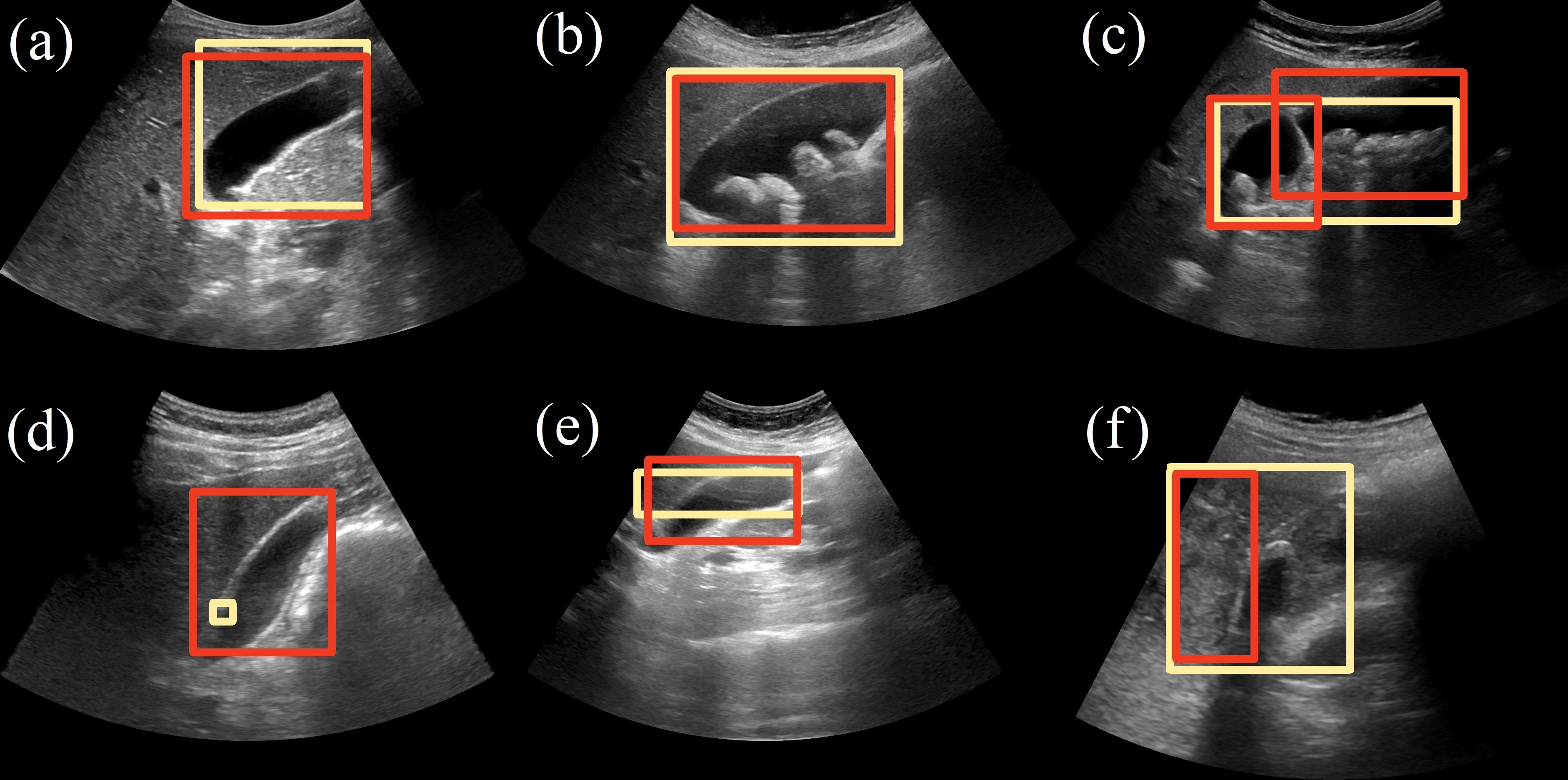
Figure 6: We visually compare roi selection by Faster-RCNN (dark red) with the roi identified by expert Radiologists (light yellow). (a, b) The predicted aroi matches well with the radiologists’ expectations. (c) The model considers the sections partitioned by the gb wall as separate regions. However, the union of the predicted boxes very closely approximates the actual gb region. (d, e) Although the radiologist made an error in judging the roi, Faster-RCNN was able to identify an accurate roi resulting in a visually superior prediction. (f) The predicted roi covers only a portion of the area an expert radiologist considered necessary. Even though the region prediction seems inferior compared to the human perception, expert radiologists corroborated that the predicted region captures the gb invading the liver, a vital visual cue to detect gbc. roi samples from other detectors are in supplementary F.

6.2 Performance of GB Region Selection Models

Tab. 2 summarizes the performance of various models for localizing the gb region. For critical tasks such as region selection for cancer detection, recall is more important than precision. Multiple predicted regions can be discarded in the second stage, but missing any potentially malignant region could be disastrous. We note that the Faster-RCNN achieves the highest mIoU out of all the models while maintaining very high recall and excellent precision. Hence, we use Faster-RCNN as the region selection model. In Fig. 6 we show the visual comparison of the gb localization results of Faster-RCNN along with the rois annotated by the expert radiologists. The model could predict the region of interest accurately in most cases. Although the model’s prediction visually differed from the radiologists in some samples, closer inspection revealed that the predicted region retains sufficient visual cues to detect malignancy.

Model	Spec.	Sens.
ResNet50	97.5 $\pm$ 2.4	82.9 $\pm$ 8.8
DenseNet121	96.8 $\pm$ 1.8	82.4 $\pm$ 2.7
MS-SoP (ours)	96.7 $\pm$ 2.7	87.1 $\pm$ 7.1

Table 3: The sensitivity and specificity of MS-SoP and two baseline classifiers on breast cancer detection from USG images. We report 5-fold cross-validation on the BUSI dataset.

Model	Orig. Test Set		Synth. Test Set
	Spec.	Sens.	Spec.	Sens.
ROI+VGG16	83.8	57.2	78.7 ($\downarrow$  6.1)	57.2
ROI+VGG16+VA	82.5	76.2	77.5 ($\downarrow$  6.1)	76.2
ROI+ResNet50	86.3	85.7	65.0 ($\downarrow$24.7)	85.7
ROI+ResNet50+VA	93.8	85.7	88.7 ($\downarrow$  5.4)	85.7
ROI+Inception-V3	56.3	83.3	41.3 ($\downarrow$26.6)	83.3
ROI+Inception-V3+VA	91.3	69.0	78.8 ($\downarrow$13.7)	69.0
GBCNet	90.0	92.9	76.2 ($\downarrow$15.3)	92.9
GBCNet+VA	95.0	97.6	85.0 ($\downarrow$10.5)	97.6

Table 4: Robustness of the curriculum in tacking texture bias while detecting gbc. We show the performance of using curriculum on four models that apply classifiers on localized gb region - (a) ROI+VGG16, (b) ROI+ResNet50, (c) ROI+Inception-V3, and (d) GBCNet (ROI+MS-SoP). The relative change (in percentage) in specificity for synthetic test data is shown within parentheses. The sensitivity remains unchanged as the malignant images were not altered. Observe that as compared to the models trained on high-resolution images, our VA-based curriculum is more robust to textures and is able to maintain a lower drop in specificity. The only exception is the ROI+VGG16 model, for which the curriculum training does not lower the drop in specificity.

6.3 Applicability of the Proposed Classifier in Breast Cancer Detection from USG Images

We explored the applicability of the proposed MS-SoP classifier on breast cancer detection from usg images for a publicly available dataset, BUSI [1], containing 133 normal, 487 benign, and 210 malignant images. The images in BUSI are already cropped from original usg images to highlight only the important regions. Thus, we skip the roi selection and run the MS-SoP classifier on BUSI. Tab. 3 shows that the MS-SoP classifier achieves much better sensitivity, which indicates the superiority of the MS-SoP architecture for malignancy identification on usg images. We note that while breast cancer detection relies on tissue/ mass characterization, gbc detection is primarily based on wall shape and mass anomaly.

6.4 Efficacy of the Proposed Curriculum

Robustness in Tackling Texture Bias: As described earlier, spurious textures present in usg images tend to increase the false positives in detecting malignancy. To validate this hypothesis, we created a synthetic test set. We used the method given by [56] and added low-level frequencies from malignant images to alter the original texture of normal and benign samples. We also manually added patches looking like soft tissue near the gb region of normal and benign images. Expert radiologists confirmed that the diagnosis of the gb pathology is not altered. Tab. 4 shows that the specificity decreases due to the increase of the false positives. The sensitivity remains unaffected as the prediction for malignant gb samples was unchanged. The network trained with the proposed curriculum tackles texture bias well and accurately predicts non-malignant samples in synthetic test data. This experiment shows that the proposed curriculum effectively tackles texture bias. Fig. 7 shows a visual sample of how the soft tissue-like texture influences the network’s decision and how the curriculum helps the network to rectify the discriminative regions.

Performance Improvement: We also assess the quantitative performance improvement of models due to the curriculum training in supplementary B.

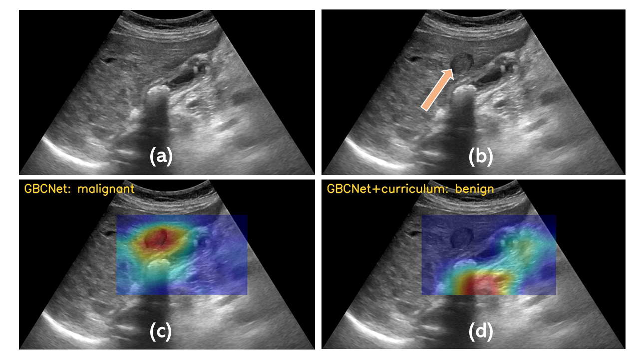
Figure 7: (a) Original image of a benign gb. The gb presents a stone and thickened wall. (b) In the synthetic image, we added an artificial tissue-like patch near the benign gb region (highlighted by the arrow). This patch is not a part of the original gb, and expert radiologists confirmed that the diagnosis of the gb is not altered. (b) The textured artificial patch makes the GBCNet biased, and it focuses on the patch to predict the sample as malignant (false-positive). (d) Visual acuity curriculum fixes the texture bias of the GBCNet and helps the network to re-adjust the salient regions to the actual gb pathology.

6.5 Ablation Study

Choice of Classifier in GBCNet: We have plugged in other deep classification networks in place of the proposed MS-SoP classifier in the GBCNet framework. Fig. 8(a) summarizes the results. The MS-SoP classifier on GBCNet provides the best gbc detection accuracy. Using the classifiers on the rois improves the sensitivity and accuracy for ResNet50 and VGG16. However, the drop in specificity results in performance degradation for Inception-V3 as the sensitivity was not improved.

Choice of Training Regime: We used the proposed GBCNet model to assess the influence of the visual acuity-based curriculum. We compare the curriculum with two possible alternatives - (i) anti-curriculum that initially trains with high resolution and progressively lowers the resolution, and (ii) control-curriculum where the samples are not sorted resolution-wise, and the curriculum contains a random set of blurred samples. Note that the control-curriculum can also be thought of using Gaussian blurring as a data augmentation where the probability of choosing a particular $\sigma$ is equal to the fraction of epochs the $\sigma$ used during the curriculum. Fig. 8(b) and 8(c) show the performance of the various curriculum strategies on the performance on GBCNet. Further, to understand how various curriculum strategies affect a model’s generalization at different resolutions, we blur the test set using different values of $\sigma$ and evaluate the models on these images (Fig. 8(d)). We see that the model trained using the proposed curriculum generalizes well across different image resolutions, which is an indicator of better spatial understanding.

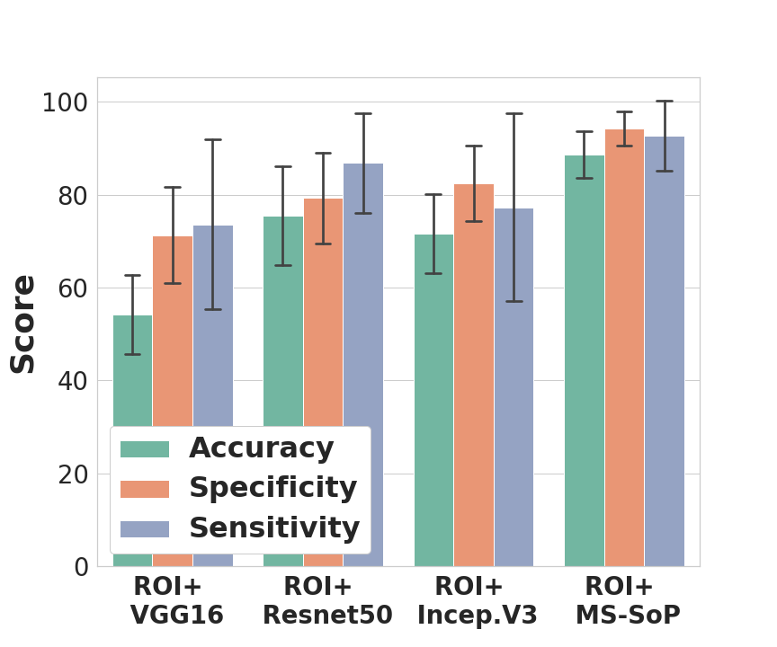
(a)

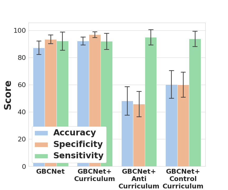
(b)

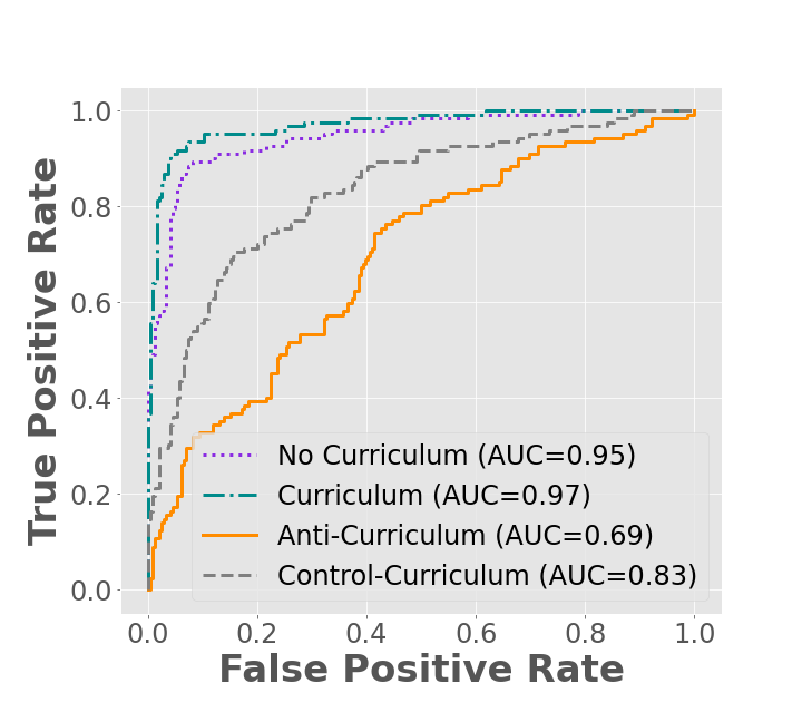
(c)

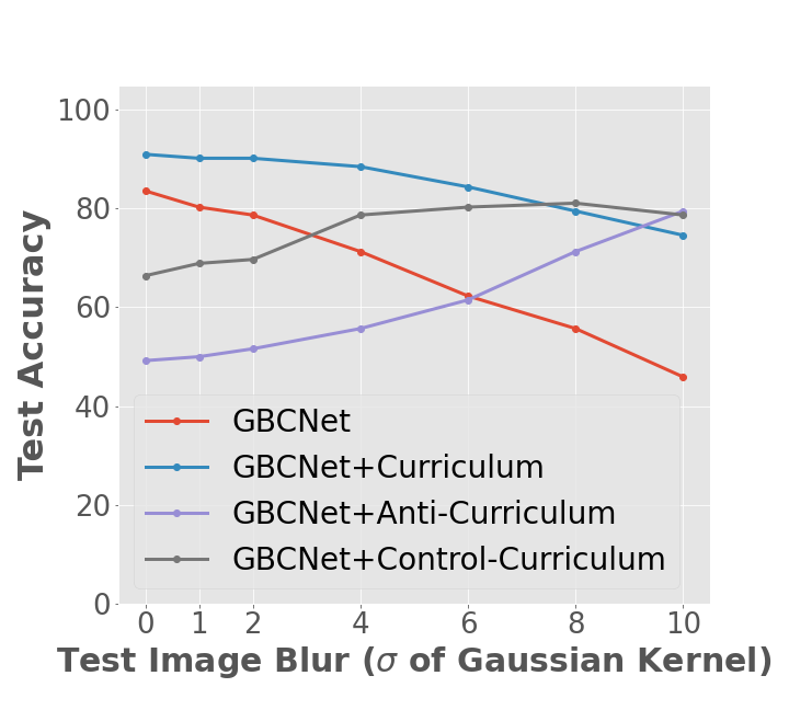
(d)

Figure 8: Ablation study. (a) Comparison of accuracy, specificity, and sensitivity for applying different classification networks (VGG16, ResNet50, Inception-V3, and MS-SoP) on the localized gb. We have reported the 10-fold cross validation results. (b) The efficacy of the proposed training regime in terms of accuracy, specificity, sensitivity. (c) ROC-AUC for different training regimes on the test set. (d) The proposed curriculum generalizes better at different resolutions.

7 Conclusion

This paper addresses Gallbladder Cancer detection from Ultrasound images using deep learning and proposes a new supervised learning framework (GBCNet) based on roi selection and multi-scale second-order pooling. The proposed design helps the classifier focus on the crucial gb region predicted by the region selection network. We propose a visual acuity-based curriculum to make our design resilient to texture bias and improve its specificity. Extensive experiments show that GBCNet, combined with curriculum learning, improves performance over the baseline deep classification and object detection architectures. We hope our work will generate interest in the community towards this important but hitherto overlooked problem of gbc detection.

Acknowledgement: The authors thank IIT Delhi HPC facility for computational resources.

Supplementary Material

Appendix A Details of Data Acquisition and Annotation

Data Acquisition: The study was approved by the ethics committee of the Postgraduate Institute of Medical Education and Research, Chandigarh. We performed all procedures according to the Declaration of Helsinki and the research guidelines of Indian Council of Medical Research. According to the hospital’s protocol, 6 hours fasting was advised a day before the Ultrasound (USG) examinations for adequate distension of the GB. Two radiologists with expertise in abdominal USG performed the examinations on a Logic S8 machine (GE Healthcare) using a convex low-frequency transducer with a frequency range of 1–5 MHz. USG assessment was done from different angles using both subcostal and intercostal views to visualize the entire GB, including the fundus, body, and neck. Patients were examined in different positions for adequate visualization of the GB. The screen area was adjusted so that the GB could occupy at least 20% of the entire screen.

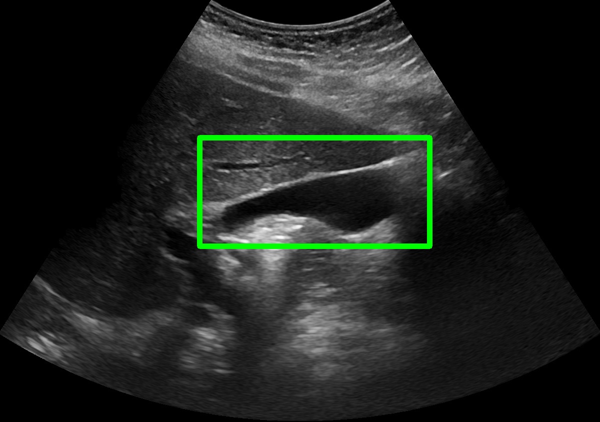
(a)

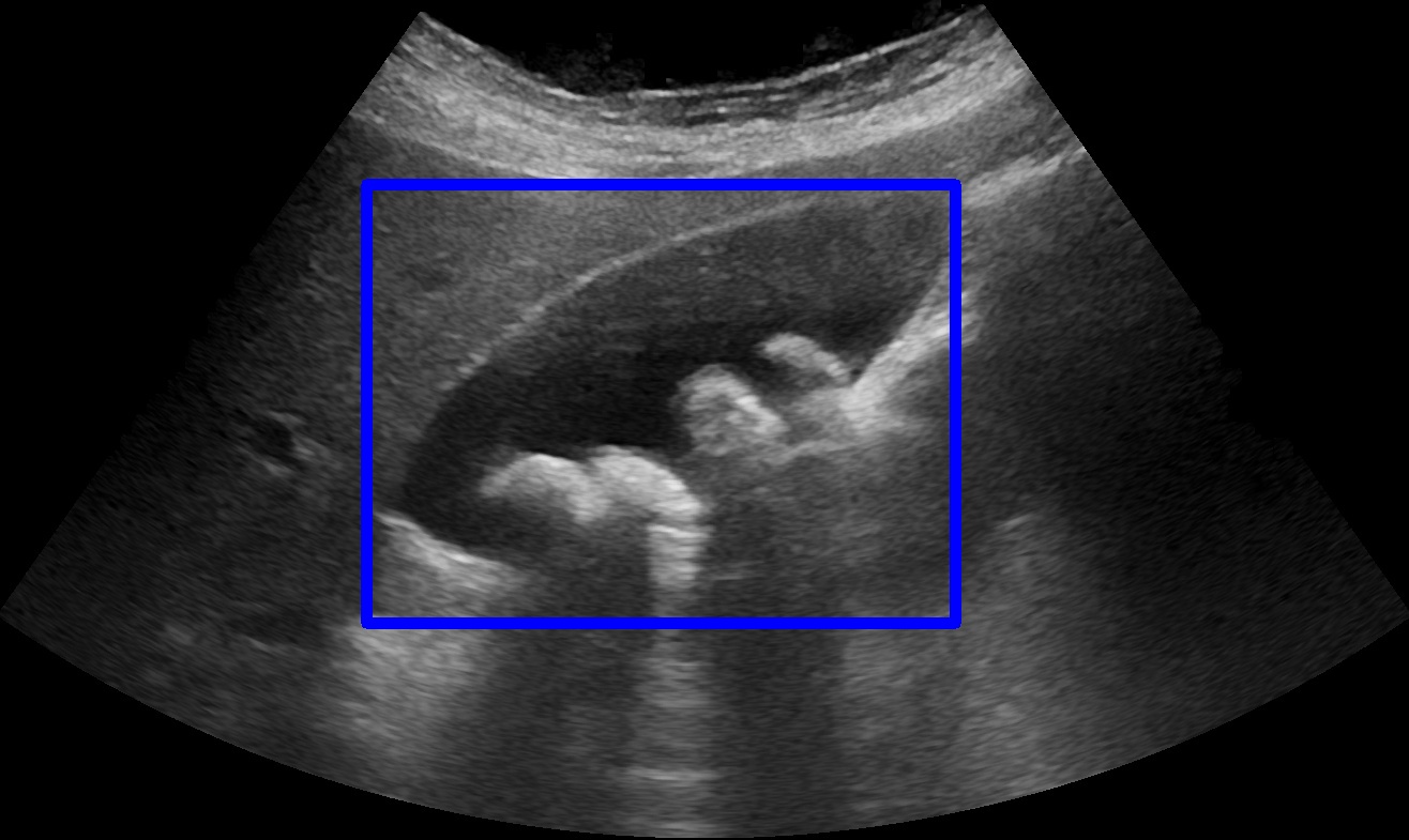
(b)

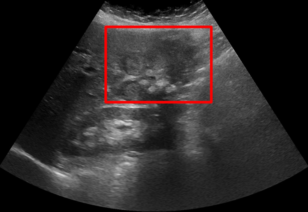
(c)

Figure S1: Sample ROI annotation. (a) Normal GB with ROI annotated in green, (b) GB with benign abnormalities with ROI in blue, and (c) Malignant GB with ROI annotated in red.

ROI Annotation: Apart from image classification labels, we used bounding-box annotations to capture the GB localization. Two radiologists with 7 and 2 years of experience in abdomen radiology did the bounding-box annotations with consensus using the LabelMe [44] software. A single free-size axis-aligned rectangular box in every image, spanning the entire GB and adjacent liver parenchyma, preferably keeping the GB in the box’s center, highlights the region of interest (see Fig. S1).

Model	Acc	Spec.	Sens.
ROI+VGG16	53.3 $\pm$ 9.2	71.9 $\pm$ 11.5	73.3 $\pm$ 17.9
ROI+VGG16+VA	77.7 $\pm$ 4.1	93.8 $\pm$ 3.0	72.0 $\pm$ 19.5
ROI+ResNet50	76.6 $\pm$ 10.7	82.3 $\pm$ 10.5	90.9 $\pm$ 11.1
ROI+ResNet50+VA	85.4 $\pm$ 7.7	92.3 $\pm$ 5.9	87.5 $\pm$ 9.1
ROI+Inception-V3	71.8 $\pm$ 8.9	83.3 $\pm$ 8.7	78.5 $\pm$ 21.4
ROI+Inception-V3+VA	82.6 $\pm$ 4.6	93.1 $\pm$ 4.4	82.6 $\pm$ 9.9
RetinaNet	74.9 $\pm$ 7.3	86.7 $\pm$ 7.8	79.1 $\pm$ 8.9
RetinaNet+VA	73.3 $\pm$ 6.0	92.1 $\pm$ 4.4	70.6 $\pm$ 14.2
GBCNet (ROI+MS-SoP)	88.2 $\pm$ 5.1	94.2 $\pm$ 3.7	92.3 $\pm$ 7.1
GBCNet+VA	92.1 $\pm$ 2.9	96.7 $\pm$ 2.3	91.9 $\pm$ 6.3

Table S1: Model performances (10-fold cross-validation) for training with our proposed visual acuity-based curriculum.

Appendix B Performance Improvement with Proposed Curriculum

We show the performance improvement of various models with the curriculum-based training in Tab. S1. All models show improvement in specificity, which indicates the effectiveness of the proposed blurring-based curriculum in tackling texture bias.

Appendix C Implementation details

Tab. S2 lists the configurations of all models which we have used. We trained on the Quadro P5000 16GB GPU. The table includes a brief description of the various stages of the network, input image sizes ($H\times W\times D$), the optimizer, relevant hyper-parameters such as learning rate, weight decay, momentum, batch size, and the number of training epochs/steps for the network.

Model	Description	Input Size	Optimizer	Batch size	Epochs/ Steps
YOLOv4 [9]	CSPDarknet53 backbone, PANet neck, anchor-based YOLO head. Total 162-layers. Backbone was frozen for first 800 step. Entire network was trainable thereafter. Single stage, anchor-based	$608\times 608\times 3$	SGD LR = 0.0001 momentum = 0.95 weight decay = 0.0005	64	3000 steps
Faster-RCNN [42]	Resnet50 Feature Pyramid backbone. Backbone was frozen for training. Two-stage, anchor-based.	$800\times 1333\times 3$	SGD LR = 0.005 momentum = 0.9 weight decay = 0.0005	16	60 epochs
Reppoints [57]	Resnet101 backbone, Group Normalization neck, and a reppoints head. Backbone was frozen for first 30 epochs, and entire network was trainable thereafter. Two-stage, anchor-free	$800\times 1333\times 3$	SGD LR = 0.001 momentum = 0.9 weight decay = 0.0001	4	50 epochs
Centripetal-Net [20]	Improvement over CornerNet model. Uses centripetal shift to match corners. HourglassNet-104 backbone. Enitre network was trainable. Anchor-free	$511\times 511\times 3$	Adam LR = 0.0005	4	50 epochs
ResNet [30]	Resnet-50 used. All layers were trainable. Output dimension of last fully connected layer is three - corresponding to normal, benign, and malignant GB. LR decays by 10% after every 5 epochs through a step LR scheduler.	$224\times 224\times 3$	SGD LR = 0.005 momentum = 0.9 weight decay = 0.0005	16	100 epochs
VGG [46]	VGG-16 is used. All layers were trainable. LR decays by 10% after every 5 epochs through a step LR scheduler.	$224\times 224\times 3$	SGD LR = 0.005 momentum = 0.9 weight decay = 0.0005	16	100 epochs
Inception [51]	Inception-V3 used. All layers were trainable. LR decays by 10% after every 5 epochs through a step LR scheduler.	$299\times 299\times 3$	SGD LR = 0.005 momentum = 0.9 weight decay = 0.0005	16	100 epochs
RetinaNet [36]	Resnet-18-FPN used as backbone. All layers were trainable. Three output classes corresponding to normal, benign, and malignant GB.	$512\times 512\times 3$	Adam LR = 0.0001	8	50 epochs
EfficientDet [52]	EfficientNet-B4 used as backbone and BiFPN as feature network. All layers were trainable. Three output classes corresponding to normal, benign, and malignant GB.	$1024\times 1024\times 3$	Adam LR = 0.001	2	50 epochs
MS-SoP Classifier (Ours)	16 MS-SoP layers. All layers were trainable. Three output classes corresponding to normal, benign, and malignant GB.	$224\times 224\times 3$	SGD LR = 0.005 momentum = 0.9 weight decay = 0.0005	16	100 epochs

Table S2: Implementation details for the different baseline networks used for classification and gallbladder localization.

Appendix D Calculating Precision and Recall for GB Localization Networks

For computing precision and recall during the GB localization phase, as suggested by [43], if the center of the predicted region lies within the bounding box of the ground truth region, then we consider a region prediction to be a true positive; otherwise, we consider the region prediction to be a false positive due to localization error. Further, we consider the zero/no region prediction as a false negative (all our images contain GB, and the localization network’s task is to merely localize it).

Appendix E GradCAM Visuals for GBCNet

Figure S2 shows the sample Grad-CAM visualizations of the predictions using GBCNet (ROI+MS-SoP) with curriculum learning.

Appendix F ROI Visuals

In figure S3, we show sample predictions of the GB region localization for different models. We also show the region of interest as perceived by the expert radiologists. The localization model is fairly accurate in capturing important regions of the USG image.

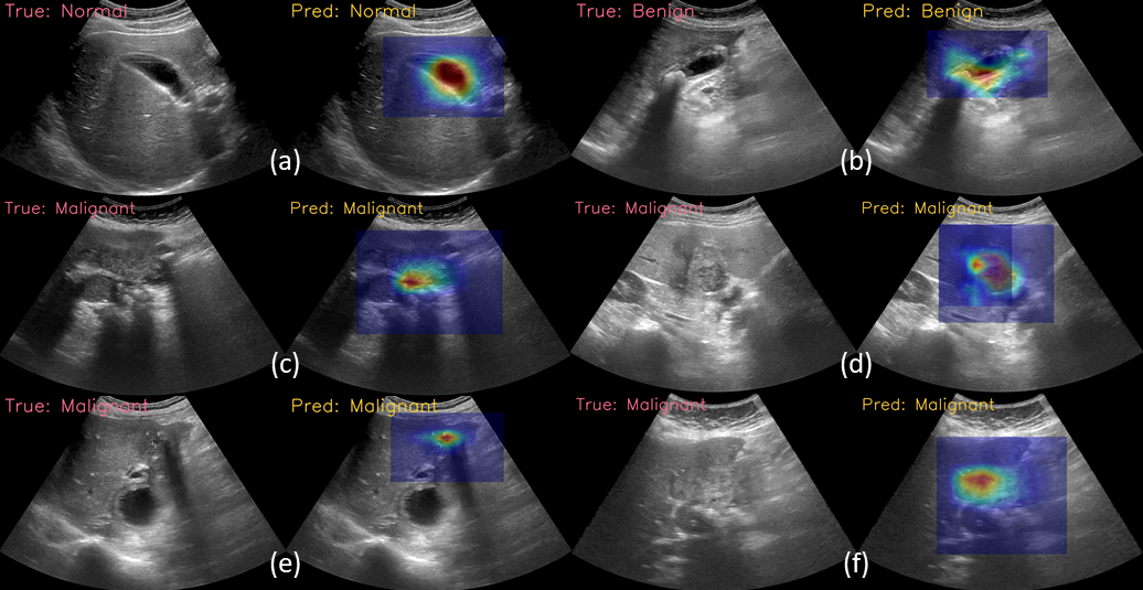
Figure S2: Sample Grad-CAM visuals of GBCNet with curriculum learning. (a) Normal, (b) Benign, and (c)–(f) Malignant samples.

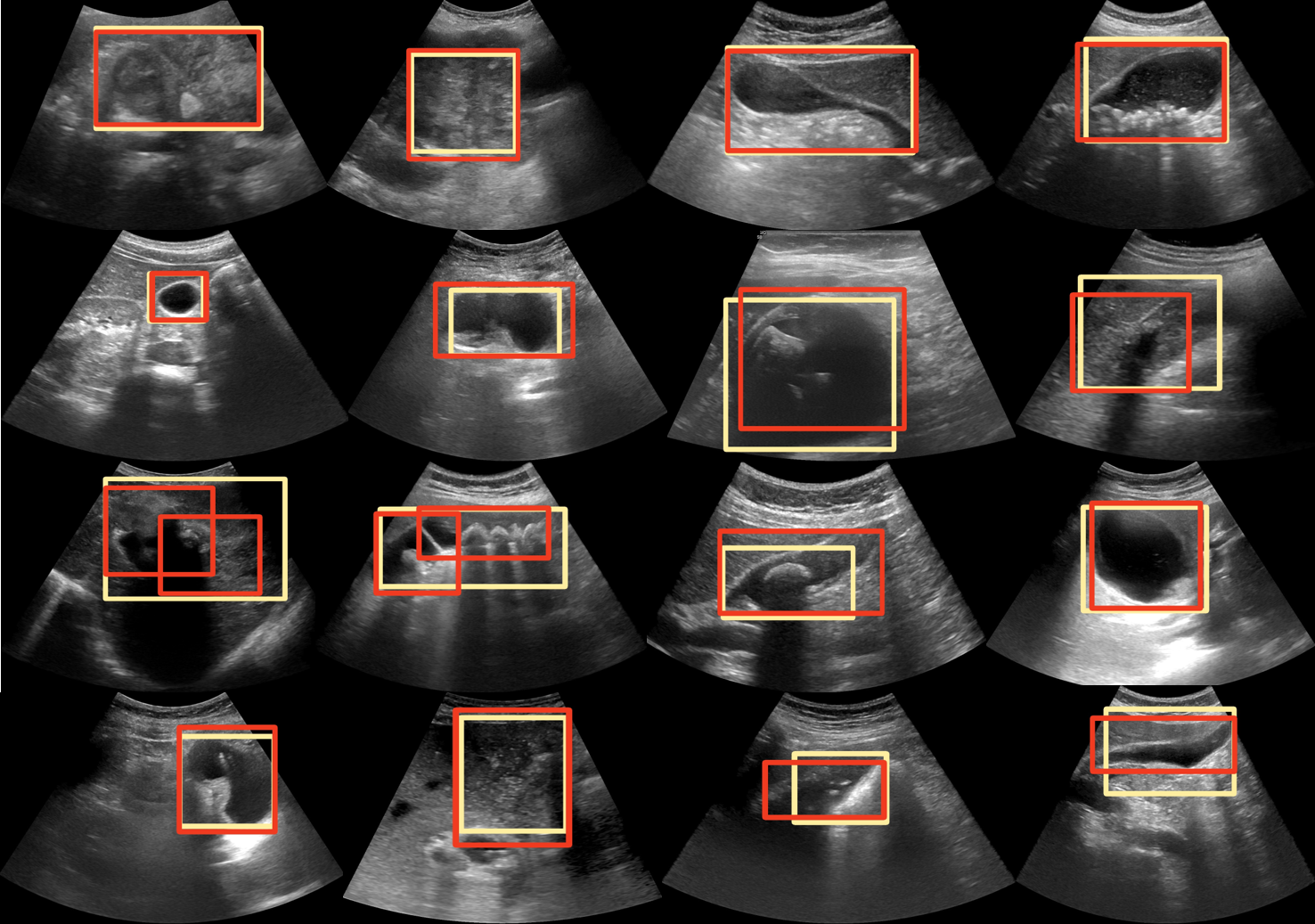
Figure S3: Sample visual results of RoI Detection models. First row - Faster-CNN, second row - YOLOv4, third row - Reppoints, and fourth row - CentripetalNet. Dark red is the ROI prediction by the model and light yellow is expert radiologists’ perception of ROI.

References

- [1] Walid Al-Dhabyani, Mohammed Gomaa, Hussien Khaled, and Aly Fahmy. Dataset of breast ultrasound images. Data in brief, 28:104863, 2020.
- [2] Laith Alzubaidi, Mohammed A Fadhel, Omran Al-Shamma, Jinglan Zhang, J Santamaría, Ye Duan, and Sameer R Oleiwi. Towards a better understanding of transfer learning for medical imaging: a case study. Applied Sciences, 10(13):4523, 2020.
- [3] Diego Ardila, Atilla P Kiraly, Sujeeth Bharadwaj, Bokyung Choi, Joshua J Reicher, Lily Peng, Daniel Tse, Mozziyar Etemadi, Wenxing Ye, Greg Corrado, et al. End-to-end lung cancer screening with three-dimensional deep learning on low-dose chest computed tomography. Nature medicine, 25(6):954–961, 2019.
- [4] Reza Azad, Abdur R Fayjie, Claude Kauffman, Ismail Ben Ayed, Marco Pedersoli, and Jose Dolz. On the texture bias for few-shot cnn segmentation. arXiv preprint arXiv:2003.04052, 2020.
- [5] Babak Ehteshami Bejnordi, Mitko Veta, Paul Johannes Van Diest, Bram Van Ginneken, Nico Karssemeijer, Geert Litjens, Jeroen AWM Van Der Laak, Meyke Hermsen, Quirine F Manson, Maschenka Balkenhol, et al. Diagnostic assessment of deep learning algorithms for detection of lymph node metastases in women with breast cancer. Jama, 318(22):2199–2210, 2017.
- [6] Babak Ehteshami Bejnordi, Mitko Veta, Paul Johannes Van Diest, Bram Van Ginneken, Nico Karssemeijer, Geert Litjens, Jeroen AWM Van Der Laak, Meyke Hermsen, Quirine F Manson, Maschenka Balkenhol, et al. Deep learning to distinguish pancreatic cancer tissue from non-cancerous pancreatic tissue: a retrospective study with cross-racial external validation. The Lancet Digital Health, 2(6):303–313, 2020.
- [7] Cheng Bian, Ran Lee, Yi-Hong Chou, and Jie-Zhi Cheng. Boundary regularized convolutional neural network for layer parsing of breast anatomy in automated whole breast ultrasound. In International Conference on Medical Image Computing and Computer-Assisted Intervention, pages 259–266. Springer, 2017.
- [8] Xiaobo Bo, Erbao Chen, Jie Wang, Lingxi Nan, Yanlei Xin, Changchen Wang, Qing Lu, Shengxiang Rao, Lifang Pang, Min Li, et al. Diagnostic accuracy of imaging modalities in differentiating xanthogranulomatous cholecystitis from gallbladder cancer. Annals of translational medicine, 7(22), 2019.
- [9] Alexey Bochkovskiy, Chien-Yao Wang, and Hong-Yuan Mark Liao. Yolov4: Optimal speed and accuracy of object detection. arXiv preprint arXiv:2004.10934, 2020.
- [10] Freddie Bray, Jacques Ferlay, Isabelle Soerjomataram, Rebecca L Siegel, Lindsey A Torre, and Ahmedin Jemal. Global cancer statistics 2018: Globocan estimates of incidence and mortality worldwide for 36 cancers in 185 countries. CA: a cancer journal for clinicians, 68(6):394–424, 2018.
- [11] Wieland Brendel and Matthias Bethge. Approximating cnns with bag-of-local-features models works surprisingly well on imagenet. arXiv preprint arXiv:1904.00760, 2019.
- [12] Samuel Budd, Matthew Sinclair, Bishesh Khanal, Jacqueline Matthew, David Lloyd, Alberto Gomez, Nicolas Toussaint, Emma C Robinson, and Bernhard Kainz. Confident head circumference measurement from ultrasound with real-time feedback for sonographers. In International Conference on Medical Image Computing and Computer-Assisted Intervention, pages 683–691. Springer, 2019.
- [13] Zhantao Cao, Lixin Duan, Guowu Yang, Ting Yue, and Qin Chen. An experimental study on breast lesion detection and classification from ultrasound images using deep learning architectures. BMC medical imaging, 19(1):51, 2019.
- [14] Tao Chen, Shaoxiong Tu, Haolu Wang, Xuesong Liu, Fenghua Li, Wang Jin, Xiaowen Liang, Xiaoqun Zhang, and Jian Wang. Computer-aided diagnosis of gallbladder polyps based on high resolution ultrasonography. Computer methods and programs in biomedicine, 185:105118, 2020.
- [15] Phillip M Cheng and Harshawn S Malhi. Transfer learning with convolutional neural networks for classification of abdominal ultrasound images. Journal of digital imaging, 30(2):234–243, 2017.
- [16] Linda C Chu, Seyoun Park, Satomi Kawamoto, Yan Wang, Yuyin Zhou, Wei Shen, Zhuotun Zhu, Yingda Xia, Lingxi Xie, Fengze Liu, et al. Application of deep learning to pancreatic cancer detection: Lessons learned from our initial experience. Journal of the American College of Radiology, 16(9):1338–1342, 2019.
- [17] Noel CF Codella, Q-B Nguyen, Sharath Pankanti, David A Gutman, Brian Helba, Allan C Halpern, and John R Smith. Deep learning ensembles for melanoma recognition in dermoscopy images. IBM Journal of Research and Development, 61(4/5):5–1, 2017.
- [18] Mary L Courage and Russell J Adams. Visual acuity assessment from birth to three years using the acuity card procedure: cross-sectional and longitudinal samples. Optometry and vision science: official publication of the American Academy of Optometry, 67(9):713–718, 1990.
- [19] J. Deng, W. Dong, R. Socher, L.-J. Li, K. Li, and L. Fei-Fei. ImageNet: A Large-Scale Hierarchical Image Database. In CVPR09, 2009.
- [20] Zhiwei Dong, Guoxuan Li, Yue Liao, Fei Wang, Pengju Ren, and Chen Qian. Centripetalnet: Pursuing high-quality keypoint pairs for object detection. In Proceedings of the IEEE/CVF Conference on Computer Vision and Pattern Recognition (CVPR), June 2020.
- [21] Deng-Ping Fan, Tao Zhou, Ge-Peng Ji, Yi Zhou, Geng Chen, Huazhu Fu, Jianbing Shen, and Ling Shao. Inf-net: Automatic covid-19 lung infection segmentation from ct images. IEEE Transactions on Medical Imaging, 39(8):2626–2637, 2020.
- [22] Shang-Hua Gao, Ming-Ming Cheng, Kai Zhao, Xin-Yu Zhang, Ming-Hsuan Yang, and Philip Torr. Res2net: A new multi-scale backbone architecture. IEEE Transactions on Pattern Analysis and Machine Intelligence, 43(2):652–662, 2021.
- [23] Zilin Gao, Jiangtao Xie, Qilong Wang, and Peihua Li. Global second-order pooling convolutional networks. In IEEE Conference on Computer Vision and Pattern Recognition, pages 3024–3033, 2019.
- [24] Robert Geirhos, Patricia Rubisch, Claudio Michaelis, Matthias Bethge, Felix A Wichmann, and Wieland Brendel. Imagenet-trained cnns are biased towards texture; increasing shape bias improves accuracy and robustness. arXiv preprint arXiv:1811.12231, 2018.
- [25] Pankaj Gupta, Usha Dutta, Pratyaksha Rana, Manphool Singhal, Ajay Gulati, Naveen Kalra, Raghuraman Soundararajan, Daneshwari Kalage, Manika Chhabra, Vishal Sharma, et al. Gallbladder reporting and data system (gb-rads) for risk stratification of gallbladder wall thickening on ultrasonography: an international expert consensus. Abdominal Radiology, pages 1–12, 2021.
- [26] Pankaj Gupta, Maoulik Kumar, Vishal Sharma, Usha Dutta, and Manavjit Singh Sandhu. Evaluation of gallbladder wall thickening: a multimodality imaging approach. Expert review of gastroenterology & hepatology, 14(6):463–473, 2020.
- [27] Pankaj Gupta, Yashi Marodia, Akash Bansal, Naveen Kalra, Praveen Kumar-M, Vishal Sharma, Usha Dutta, and Manavjit Singh Sandhu. Imaging-based algorithmic approach to gallbladder wall thickening. World journal of gastroenterology, 26(40):6163, 2020.
- [28] Pankaj Gupta, Kesha Meghashyam, Yashi Marodia, Vikas Gupta, Rajender Basher, Chandan Krushna Das, Thakur Deen Yadav, Santhosh Irrinki, Ritambhra Nada, and Usha Dutta. Locally advanced gallbladder cancer: a review of the criteria and role of imaging. Abdominal Radiology, 46(3):998–1007, 2021.
- [29] Zhongyi Han, Benzheng Wei, Yuanjie Zheng, Yilong Yin, Kejian Li, and Shuo Li. Breast cancer multi-classification from histopathological images with structured deep learning model. Scientific reports, 7(1):1–10, 2017.
- [30] Kaiming He, Xiangyu Zhang, Shaoqing Ren, and Jian Sun. Deep residual learning for image recognition. In Proceedings of the IEEE conference on computer vision and pattern recognition, pages 770–778, 2016.
- [31] Younbeom Jeong, Jung Hoon Kim, Hee-Dong Chae, Sae-Jin Park, Jae Seok Bae, Ijin Joo, and Joon Koo Han. Deep learning-based decision support system for the diagnosis of neoplastic gallbladder polyps on ultrasonography: preliminary results. Scientific Reports, 10(1):1–10, 2020.
- [32] Andrew Jesson, Nicolas Guizard, Sina Hamidi Ghalehjegh, Damien Goblot, Florian Soudan, and Nicolas Chapados. Cased: curriculum adaptive sampling for extreme data imbalance. In International Conference on Medical Image Computing and Computer-Assisted Intervention, pages 639–646. Springer, 2017.
- [33] MiYoung Kwon, Rong Liu, and Lillian Chien. Compensation for blur requires increase in field of view and viewing time. PLoS One, 11(9):e0162711, 2016.
- [34] Peihua Li, Jiangtao Xie, Qilong Wang, and Wangmeng Zuo. Is second-order information helpful for large-scale visual recognition? In IEEE international conference on computer vision, pages 2070–2078, 2017.
- [35] Jing Lian, Yide Ma, Yurun Ma, Bin Shi, Jizhao Liu, Zhen Yang, and Yanan Guo. Automatic gallbladder and gallstone regions segmentation in ultrasound image. International journal of computer assisted radiology and surgery, 12(4):553–568, 2017.
- [36] Tsung-Yi Lin, Priya Goyal, Ross Girshick, Kaiming He, and Piotr Dollár. Focal loss for dense object detection. In Proc. IEEE ICCV, pages 2980–2988, 2017.
- [37] Tsung-Yi Lin, Michael Maire, Serge Belongie, Lubomir Bourdev, Ross Girshick, James Hays, Pietro Perona, Deva Ramanan, C. Lawrence Zitnick, and Piotr Dollár. Microsoft coco: Common objects in context, 2015.
- [38] Zhenyuan Ning, Chao Tu, Qing Xiao, Jiaxiu Luo, and Yu Zhang. Multi-scale gradational-order fusion framework for breast lesions classification using ultrasound images. In International Conference on Medical Image Computing and Computer-Assisted Intervention, pages 171–180. Springer, 2020.
- [39] Ilkay Oksuz, Bram Ruijsink, Esther Puyol-Antón, James R Clough, Gastao Cruz, Aurelien Bustin, Claudia Prieto, Rene Botnar, Daniel Rueckert, Julia A Schnabel, et al. Automatic cnn-based detection of cardiac mr motion artefacts using k-space data augmentation and curriculum learning. Medical image analysis, 55:136–147, 2019.
- [40] Shanchen Pang, Tong Ding, Sibo Qiao, Fan Meng, Shuo Wang, Pibao Li, and Xun Wang. A novel yolov3-arch model for identifying cholelithiasis and classifying gallstones on ct images. PloS one, 14(6):e0217647, 2019.
- [41] Giorgia Randi, Silvia Franceschi, and Carlo La Vecchia. Gallbladder cancer worldwide: geographical distribution and risk factors. International journal of cancer, 118(7):1591–1602, 2006.
- [42] Shaoqing Ren, Kaiming He, Ross Girshick, and Jian Sun. Faster r-cnn: Towards real-time object detection with region proposal networks. In C. Cortes, N. D. Lawrence, D. D. Lee, M. Sugiyama, and R. Garnett, editors, Advances in Neural Information Processing Systems 28, pages 91–99. Curran Associates, Inc., 2015.
- [43] Dezső Ribli, Anna Horváth, Zsuzsa Unger, Péter Pollner, and István Csabai. Detecting and classifying lesions in mammograms with deep learning. Scientific reports, 8(1):1–7, 2018.
- [44] Bryan C Russell, Antonio Torralba, Kevin P Murphy, and William T Freeman. Labelme: a database and web-based tool for image annotation. International journal of computer vision, 77(1-3):157–173, 2008.
- [45] Ramprasaath R Selvaraju, Michael Cogswell, Abhishek Das, Ramakrishna Vedantam, Devi Parikh, and Dhruv Batra. Grad-cam: Visual explanations from deep networks via gradient-based localization. In Proceedings of the IEEE international conference on computer vision, pages 618–626, 2017.
- [46] Karen Simonyan and Andrew Zisserman. Very deep convolutional networks for large-scale image recognition. arXiv preprint arXiv:1409.1556, 2014.
- [47] Samarth Sinha, Animesh Garg, and Hugo Larochelle. Curriculum by smoothing, 2020.
- [48] Korsuk Sirinukunwattana, Shan E Ahmed Raza, Yee-Wah Tsang, David RJ Snead, Ian A Cree, and Nasir M Rajpoot. Locality sensitive deep learning for detection and classification of nuclei in routine colon cancer histology images. IEEE transactions on medical imaging, 35(5):1196–1206, 2016.
- [49] Fraser W Smith and Philippe G Schyns. Smile through your fear and sadness: transmitting and identifying facial expression signals over a range of viewing distances. Psychological Science, 20(10):1202–1208, 2009.
- [50] Zahra Sobhaninia, Shima Rafiei, Ali Emami, Nader Karimi, Kayvan Najarian, Shadrokh Samavi, and SM Reza Soroushmehr. Fetal ultrasound image segmentation for measuring biometric parameters using multi-task deep learning. In 2019 41st Annual International Conference of the IEEE Engineering in Medicine and Biology Society (EMBC), pages 6545–6548. IEEE, 2019.
- [51] Christian Szegedy, Vincent Vanhoucke, Sergey Ioffe, Jon Shlens, and Zbigniew Wojna. Rethinking the inception architecture for computer vision. In Proceedings of the IEEE conference on computer vision and pattern recognition, pages 2818–2826, 2016.
- [52] Mingxing Tan, Ruoming Pang, and Quoc V Le. Efficientdet: Scalable and efficient object detection. In Proc. IEEE CVPR, pages 10781–10790, 2020.
- [53] Yuxing Tang, Xiaosong Wang, Adam P Harrison, Le Lu, Jing Xiao, and Ronald M Summers. Attention-guided curriculum learning for weakly supervised classification and localization of thoracic diseases on chest radiographs. In International Workshop on Machine Learning in Medical Imaging, pages 249–258. Springer, 2018.
- [54] Lukas Vogelsang, Sharon Gilad-Gutnick, Evan Ehrenberg, Albert Yonas, Sidney Diamond, Richard Held, and Pawan Sinha. Potential downside of high initial visual acuity. Proceedings of the National Academy of Sciences, 115(44):11333–11338, 2018.
- [55] Tao Wang, Yu Li, Bingyi Kang, Junnan Li, Junhao Liew, Sheng Tang, Steven Hoi, and Jiashi Feng. The devil is in classification: A simple framework for long-tail instance segmentation. In European Conference on computer vision, pages 728–744. Springer, 2020.
- [56] Yanchao Yang and Stefano Soatto. Fda: Fourier domain adaptation for semantic segmentation. In Proceedings of the IEEE/CVF Conference on Computer Vision and Pattern Recognition, pages 4085–4095, 2020.
- [57] Ze Yang, Shaohui Liu, Han Hu, Liwei Wang, and Stephen Lin. Reppoints: Point set representation for object detection. In The IEEE International Conference on Computer Vision (ICCV), Oct 2019.
- [58] Moi Hoon Yap, Manu Goyal, Fatima M Osman, Robert Martí, Erika Denton, Arne Juette, and Reyer Zwiggelaar. Breast ultrasound lesions recognition: end-to-end deep learning approaches. Journal of medical imaging, 6(1):011007, 2018.
- [59] Hai-Xia Yuan, Wen-Ping Wang, Pei-Shan Guan, Le-Wu Lin, Jie-Xian Wen, Qing Yu, and Xue-Jun Chen. Contrast-enhanced ultrasonography in differential diagnosis of focal gallbladder adenomyomatosis and gallbladder cancer. Clinical Hemorheology and Microcirculation, 70(2):201–211, 2018.
- [60] Lei Zhang, Jian Huang, and Li Liu. Improved deep learning network based in combination with cost-sensitive learning for early detection of ovarian cancer in color ultrasound detecting system. Journal of medical systems, 43(8):1–9, 2019.
- [61] Lei Zhu, Rongzhen Chen, Huazhu Fu, Cong Xie, Liansheng Wang, Liang Wan, and Pheng-Ann Heng. A second-order subregion pooling network for breast lesion segmentation in ultrasound. In International Conference on Medical Image Computing and Computer-Assisted Intervention, pages 160–170. Springer, 2020.
- [62] Georgios Zoumpourlis, Alexandros Doumanoglou, Nicholas Vretos, and Petros Daras. Non-linear convolution filters for cnn-based learning. In Proceedings of the IEEE international conference on computer vision, pages 4761–4769, 2017.