KMT-2021-BLG-1898: Planetary microlensing event involved with binary source stars

Abstract

Aims. The light curve of the microlensing event KMT-2021-BLG-1898 exhibits a short-term central anomaly with double-bump features that cannot be explained by the usual binary-lens or binary-source interpretations. With the aim of interpreting the anomaly, we analyze the lensing light curve under various sophisticated models.

Methods. We find that the anomaly is explained by a model, in which both the lens and source are binaries (2L2S model). For this interpretation, the lens is a planetary system with a planet/host mass ratio of $q\sim 1.5\times 10^{-3}$, and the source is a binary composed of a turn off or a subgiant star and a mid K dwarf. The double-bump feature of the anomaly can also be depicted by a triple-lens model (3L1S model), in which the lens is a planetary system containing two planets. Among the two interpretations, the 2L2S model is favored over the 3L1S model not only because it yields a better fit to the data, by $\Delta\chi^{2}=[14.3$–18.5], but also the Einstein radii derived independently from the two stars of the binary source result in consistent values. According to the 2L2S interpretation, KMT-2021-BLG-1898 is the third planetary lensing event occurring on a binary stellar system, following MOA-2010-BLG-117 and KMT-2018-BLG-1743.

Results. Under the 2L2S interpretation, we identify two solutions resulting from the close-wide degeneracy in determining the planet-host separation. From a Bayesian analysis, we estimate that the planet has a mass of $\sim 0.7$–0.8 $M_{\rm J}$, and it orbits an early M dwarf host with a mass of $\sim 0.5\leavevmode\nobreak\ M_{\odot}$. The projected planet-host separation is $\sim 1.9$ AU and $\sim 3.0$ AU according to the close and wide solutions, respectively.

1 Introduction

Microlensing planets are detected and characterized by analyzing short-term anomalies in lensing light curves induced by planets. In most cases, planetary anomalies are well described by a binary-lens single-source (2L1S) model, in which the lens is composed of two masses (planet and its host) and the source is a single star. However, some planetary signals are deformed from the 2L1S form due to various causes. The first major cause for such a deformation is the existence of an extra lens component. This additional lens component can be a second planet, as in the cases of OGLE-2006-BLG-109 (Gaudi et al., 2008; Bennett et al., 2010), OGLE-2012-BLG-0026 (Han et al., 2013), and OGLE-2018-BLG-1011 (Han et al., 2019), or a binary companion to the host, as in the cases of OGLE-2007-BLG-349 (Bennett et al., 2016), KMT-2020-BLG-0414 (Zang et al., 2021), OGLE-2016-BLG-0613 (Han et al., 2017), and OGLE-2018-BLG-1700 (Han et al., 2020). Another major cause of a deformation is the binarity of the source, as illustrated by the lensing events MOA-2010-BLG-117 (Bennett et al., 2018) and KMT-2018-BLG-1743 (Han et al., 2021a). For the lensing event KMT-2019-BLG-1715, an even more complicated model with three lens masses (binary stars and a planet) and two source stars is needed to explain the deformed anomalies in the lensing light curve (Han et al., 2021c).

Interpreting a deformed planetary anomaly is a difficult task because of the complexity of modeling with the increased number of lensing parameters. Even in the simplest case of a single planetary event, seven basic parameters are needed to describe the observed light curve. Considering an extra lens component (3L1S) or a source component (2L2S) in modeling requires one to include multiple extra parameters in addition to the basic parameters, and this results in the complexity in modeling. We give an explanation of the lensing parameters for the individual models (2L1S, 3L1S, and 2L2S) in the analysis part of the paper. As a result, some planetary signals with complex structures may be missed due to the difficulty of modeling. For example, the planetary nature of the lensing events OGLE-2018-BLG-1700, KMT-2018-BLG-1743, and KMT-2019-BLG-1715 had not been known before they were reanalyzed with complex models from the systematic reinvestigation of anomalous events with no presented lensing models. Considering that planet statistics are based on the detection efficiency, which is estimated as the ratio of lensing events with detected planetary signals to the total number of lensing events, missing planets would lead to erroneous planet statistics such as the planet frequency and demographic distribution.

In this work, we report a planet found from the analysis of the microlensing event KMT-2021-BLG-1898. A short-term anomaly appeared near the peak of the lensing light curve, but it cannot be described by the usual binary-lens or binary-source (1L2S) model. We investigate various causes for the deformation of the anomaly to reveal the nature of the anomaly.

We present the analysis of the planetary event according to the following organization. In Sect. 2, we give an explanation of the data, including observations, facilities, and data reductions. In Sect. 3, we describe the detailed features of the anomaly, and demonstrate the difficulty of describing the anomaly with the usual 2L1S or 1L2S models. We check the feasibility of describing the anomaly with various sophisticated models and present the analyses. We estimate the angular Einstein radius by specifying the source in Sect. 4, and estimate the physical parameters of the planet system in Sect. 5. We summarize the results and conclude in Sect. 6.

2 Observations and data

The source of the lensing event KMT-2021-BLG-1898 lies toward the Galactic bulge field with equatorial coordinates (R.A., decl.)${}_{\rm J2000}=$(17:42:46.05, -27:22:33.02), which correspond to the galactic coordinates $(l,b)=(1^{\circ}\hskip-2.0pt.000,1^{\circ}\hskip-2.0pt.353)$. Due to the proximity of the source to the Galactic center, the extinction toward the field, $A_{I}=3.56$, is fairly high. The magnitude of the baseline object is $i=20.64$ as reported in DECam catalog of Schlafly et al. (2018).

The lensing event was detected from the survey conducted by the Korea Microlensing Telescope Network (KMTNet; Kim et al., 2016) team during the 2021 bulge season. The event reached a relatively high magnification, $A_{\rm peak}\sim 63$, at the peak on 2021 July 26 (${\rm HJD}^{\prime}\equiv{\rm HJD}-2450000\sim 9421.6$). The peak region of a high-magnification is susceptible to deviations induced by a planetary companion (Griest & Safizadeh, 1998), and a short-term anomaly was actually found in the data collected by the KMTNet survey. Had the event been alerted before the peak, the anomaly could have been densely resolved by follow-up observations utilizing multiple telescopes, but no follow-up observation could be conducted because the event was alerted just after the peak. Furthermore, there are no data from the other surveys because the telescope of the OGLE survey was shut down in the 2021 season and the MOA survey did not find the event. We give a detailed description of the anomaly features in the following section.

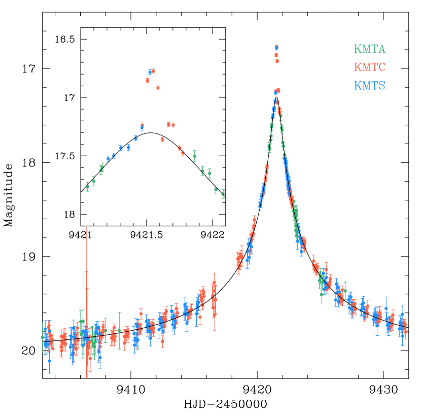
Figure 1: Light curve of KMT-2021-BLG-1898 constructed by combining the three data sets of the KMTNet telescopes: KMTA, KMTC, and KMTS. The inset shows the zoom-in view of the peak region exhibiting an anomaly feature. The curve drawn over the data point is a 1L1S model obtained by excluding the data points in the anomaly region. The colors of the data points are set to mach those of the telescopes marked in the legend.

Observations of the event were done utilizing the three telescopes of the KMTNet survey. The telescopes are identical with a 1.6 m aperture, and they are globally distributed in the three continents of the Southern Hemisphere for continuous coverage of lensing events. The sites of the individual telescopes are the Siding Spring Observatory (KMTA) in Australia, the Cerro Tololo Inter-American Observatory (KMTC) in South America, and the South African Astronomical Observatory (KMTS) in Africa. Each telescope is equipped with a wide-field camera yielding 4 deg² field of view. The lensing event is in the KMT18 field, toward which observations were conducted with a 1 hr cadence. Images of the field were mostly acquired in the $I$ band, but 9% of the images were obtained in the $V$ band for the source color measurement. We discuss the procedure of the source color measurement in Sect. 4.

Photometry of the lensing event was done using the KMTNet pipeline (Albrow et al., 2009), which applies the difference image method (Tomaney & Crotts, 1996; Alard & Lupton, 1998). For a subset of the KMTC $I$- and $V$-band data, additional photometry was done using the pyDIA software (Albrow, 2017) to construct a color-magnitude (CMD) of stars around the source and estimate the source location on the CMD. For the data used in the analysis, we readjust the error bars following the routine described in Yee et al. (2012), that is, $\sigma=k(\sigma_{\rm min}+\sigma_{0})^{1/2}$, where $\sigma_{0}$ is the error estimated by the photometry pipeline, $\sigma_{\rm min}$ is a factor used to make the error to be consistent with the scatter of data, and $k$ is a scaling factor used to make $\chi^{2}$ per degree of freedom unity. These factors are $(k,\sigma_{\rm min}/{\rm mag})=(1.432,0.020)$, $(1.183,0.015)$, and $(0.872,0.020)$ for the KMTA, KMTC, and KMTS data sets, respectively.

3 Interpretation of the anomaly

Figure 1 shows the light curve of KMT-2021-BLG-1898 constructed by combining the data sets from the three KMTNet telescopes. Drawn over the data points is a model curve obtained from a single-lens single-source (1L1S) fit to the data. As shown in the inset, the peak region exhibits a brief deviation from the 1L1S light curve. The 1L1S fitting yields lensing parameters of $(t_{0},u_{0},t_{\rm E})\sim(9421.5,0.016,22\leavevmode\nobreak\ {\rm days})$, where $t_{0}$ represents the time of the closest lens-source approach (expressed in ${\rm HJD}^{\prime}$), $u_{0}$ is the lens-source separation (scaled to the angular Einstein radius $\theta_{\rm E}$) at that time, and $t_{\rm E}$ represents the event time scale. An enlarged view of the peak region is presented in Figure 2 to better show the detailed features of the anomaly. The anomaly, which lasted for about 8 hours, appears to be composed of two bumps centered at ${\rm HJD}^{\prime}\sim 9421.54$ (major bump) and $\sim 9421.68$ (minor bump). The major bump was covered by the combination of the KMTS and KMTC data sets, and the minor bump was covered by the KMTC data set.

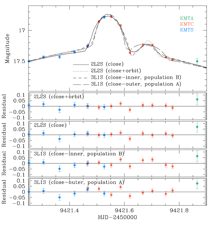
Figure 2: Zoom-in view around the peak of the light curve. The four curves drawn over the data points are the two 2L2S and two 3L1S models. One of the 2L2L (labeled as “close+orbit”) model is obtained considering the orbital motion of the binary source, while the other model (“close”) is found without considering the source orbital motion. The four lower panels show the residuals from the individual models.

3.1 2L1S and 1L2S interpretations

Table 1: 3L1S lensing parameters (population A)

Parameter	close-outer	close-inner	wide-outer	wide-inner
$\chi^{2}$	$639.5$	$640.2$	$640.0$	$640.0$
$t_{0}$ (HJD′)	$9421.535\pm 0.003$	$9421.535\pm 0.003$	$9421.536\pm 0.003$	$9421.535\pm 0.003$
$u_{0}$	$0.015\pm 0.001$	$0.014\pm 0.001$	$0.014\pm 0.001$	$0.015\pm 0.002$
$t_{\rm E}$ (days)	$23.87\pm 2.33$	$24.38\pm 2.42$	$24.06\pm 2.23$	$23.47\pm 3.17$
$s_{2}$	$0.776\pm 0.008$	$0.773\pm 0.010$	$1.288\pm 0.012$	$1.282\pm 0.012$
$q_{2}$ ($10^{-3}$)	$1.192\pm 0.172$	$1.211\pm 0.203$	$1.097\pm 0.143$	$1.093\pm 0.182$
$\alpha$ (rad)	$4.695\pm 0.010$	$4.696\pm 0.010$	$4.696\pm 0.010$	$4.692\pm 0.011$
$s_{3}$	$0.952\pm 0.013$	$1.068\pm 0.015$	$0.957\pm 0.015$	$1.053\pm 0.015$
$q_{3}$ ($10^{-5}$)	$7.87\pm 2.08$	$8.10\pm 1.78$	$6.96\pm 2.03$	$6.56\pm 2.15$
$\psi$ (rad)	$5.792\pm 0.010$	$5.782\pm 0.010$	$5.795\pm 0.011$	$5.796\pm 0.011$
$\rho$ ($10^{-3}$)	$2.45\pm 0.29$	$2.50\pm 0.28$	$2.47\pm 0.30$	$2.56\pm 0.38$
$I_{\rm S,KMT}$ (mag)	$21.83\pm 0.11$	$21.85\pm 0.11$	$21.84\pm 0.11$	$21.82\pm 0.14$

Table 2: 3L1S lensing parameters (population B)

Parameter	close-outer	close-inner	wide-outer	wide-inner
$\chi^{2}$	$636.1$	$636.0$	$636.7$	$637.7$
$t_{0}$ (HJD′)	$9421.536\pm 0.003$	$9421.536\pm 0.003$	$9421.534\pm 0.003$	$9421.536\pm 0.003$
$u_{0}$	$0.015\pm 0.002$	$0.015\pm 0.001$	$0.015\pm 0.001$	$0.016\pm 0.002$
$t_{\rm E}$ (days)	$23.55\pm 3.15$	$23.42\pm 1.87$	$23.29\pm 2.20$	$22.27\pm 2.57$
$s_{2}$	$0.750\pm 0.026$	$0.769\pm 0.026$	$1.313\pm 0.032$	$1.309\pm 0.049$
$q_{2}$ ($10^{-3}$)	$1.501\pm 0.316$	$1.464\pm 0.269$	$1.409\pm 0.210$	$1.542\pm 0.307$
$\alpha$ (rad)	$4.651\pm 0.011$	$4.645\pm 0.010$	$4.642\pm 0.010$	$4.645\pm 0.010$
$s_{3}$	$0.986^{+0.001}_{-0.010}$	$0.997^{+0.010}_{-0.001}$	$0.985^{+0.002}_{-0.007}$	$0.996^{+0.011}_{-0.001}$
$q_{3}$ ($10^{-5}$)	$4.78\pm 1.35$	$5.45\pm 1.25$	$5.21\pm 1.04$	$6.10\pm 1.35$
$\psi$ (rad)	$3.031\pm 0.011$	$3.042\pm 0.011$	$3.039\pm 0.011$	$3.051\pm 0.012$
$\rho$ ($10^{-3}$)	$2.78\pm 0.34$	$2.82\pm 0.24$	$2.82\pm 0.25$	$2.87\pm 0.31$
$I_{\rm S,KMT}$ (mag)	$21.82\pm 0.14$	$21.81\pm 0.09$	$21.81\pm 0.10$	$21.75\pm 0.11$

To investigate the origin of the anomaly, we first conducted modeling of the observed light curve under the two interpretations that the lens is a binary (2L1S model) in one interpretation and the source is a binary (1L2S model) in the other interpretation. Both the 2L1S and 1L2S models require one to include extra parameters in addition to those of the 1L1S model, that is, $(t_{0},u_{0},t_{\rm E})$. These extra parameters for the 2L1S model are $(s,q,\alpha,\rho)$, which represent the projected separation (scaled to $\theta_{\rm E}$) and mass ratio between the binary lens component, $M_{1}$ and $M_{2}$, the angle between the source motion and the binary lens axis (source trajectory angle), and the ratio of the angular source radius $\theta_{*}$ to $\theta_{\rm E}$ (normalized source radius), respectively. The normalized source radius is needed to account for the deformation of an anomaly caused by finite-source effects because 2L1S light curves are often involved with caustics (Bennett & Rhie, 1996). The extra parameters for the 1L2S model include $(t_{0,2},u_{0,2},\rho_{2},q_{F})$, which indicate the closest approach time, separation, and normalized radius of the second source, and the flux ratio between the binary source stars, $S_{1}$ and $S_{2}$, respectively (Hwang et al., 2013).

The modeling was done using the combination of a grid search and a downhill approach. In the 2L1S modeling, we divided the lensing parameters into two groups, in which the parameters $s$ and $q$ of the first group were searched for using a grid approach, while the other parameters in the second group were found using a downhill approach. We applied the Markov Chain Monte Carlo (MCMC) method for the downhill approach. We identified local solutions from the inspection of the $\Delta\chi^{2}$ map on the $\log s$–$\log q$ parameter plane constructed from the grid search, and we then refined the individual local solutions by releasing all parameters as free parameters. For the 1L2S model, all parameters were searched for using a downhill approach, in which the initial values of the lensing parameters were given considering the times and magnitudes of the anomaly features. From the modeling under the 2L1S and 1L2S interpretations, it was found that neither of the models could explain the double-bump features of the anomaly, although both models could approximately describe one of the two bumps.

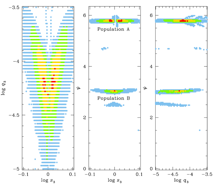
Figure 3: Maps of $\Delta\chi^{2}$ on the $\log s_{3}$–$\log q_{3}$–$\psi$ parameter planes obtained from the 3L1S modeling. Color coding is set to represent points with $\Delta\chi^{2}\leq 1n\sigma$ (red), $\leq 2n\sigma$ (yellow), $\leq 3n\sigma$ (green), and $\leq 4n\sigma$ (cyan), where $n=2$.

3.2 3L1S interpretation

Recognizing the inadequacy of the 2L1S and 1L2S models in describing the anomaly, we first checked the interpretation that the lens is composed of three masses ($M_{1}$, $M_{2}$, and $M_{3}$). We examined the 3L1S interpretation due to the combination of the two facts; first, one of the bumps can be explained by a 2L1S model with a planet-mass lens companion, and second, the anomaly appears near the peak of the light curve. If the lens contains a tertiary component, which can be either a second planet lying in the vicinity of the Einstein ring (Gaudi et al., 1998) or a binary companion to the host of the planet with a very close or a wide separation from the host (Lee et al., 2008), the tertiary lens component induce an extra caustic in the central magnification region, and the second bump, which could not be described with a single-planetary model, may be explained by a 3L1S model.

For a 3L1S modeling, extra parameters are needed in addition to those of a 2L1S modeling. These extra parameters are $(s_{3},q_{3},\psi)$, which represent the separation and mass ratio between $M_{1}$ and $M_{3}$, and the orientation angle of $M_{3}$ as measured from the $M_{1}$–$M_{2}$ axis with a center at the position of $M_{1}$. In the 3L1S model, we designate the parameters related to $M_{2}$ as $(s_{2},q_{2})$ to distinguish them from the parameters related to $M_{3}$.

It is known that anomalies in the central magnification region can often be approximately described by the superposition of the anomalies induced by the two $M_{1}$–$M_{2}$ and $M_{1}$–$M_{3}$ binary pairs (Bozza, 1999; Han et al., 2001). Under this approximation, we conducted a 3L1S modeling according to the following procedure. In the first step, we conducted a grid searches for $(s_{3},q_{3},\psi)$ by fixing the other lensing parameters as the values of the 2L1S model describing the major bump. We checked local solutions on the three $\log s_{3}$–$\log q_{3}$–$\psi$ parameter planes, and then polished the individual local solutions identified from the first-round grid search by allowing all parameters to vary.

Figure 3 shows the $\Delta\chi^{2}$ maps on the $\log s_{3}$–$\log q_{3}$–$\psi$ parameter planes obtained from the grid search. We identified two distinctive populations of local solutions caused by the accidental degeneracy in determining $\psi$: solutions in “population A” with $\psi\sim 330^{\circ}$ and solutions in “population B” with $\psi\sim 173^{\circ}$. For each population, there are four degenerate solutions resulting from degeneracies in determining the separations $s_{2}$ ($M_{1}$–$M_{2}$ degeneracy) and $s_{3}$ ($M_{1}$–$M_{3}$ degeneracy), and thus there exist eight solutions in total. These degeneracies will be further discussed below. Figures 4 and 5 show the lens system configurations of the individual 3L1S models in the A and B populations, respectively.

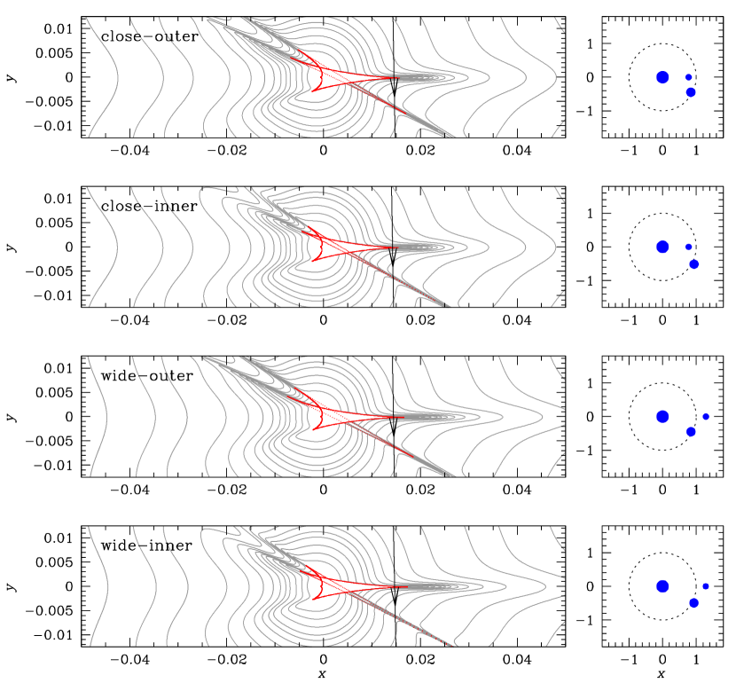
Figure 4: Lens system configurations of the four 3L1S models in the population A. For each model, the left panel shows the caustic (red cuspy figure) and source trajectory (line with an arrow) in the central magnification region, and the right panel shows the positions of the lens components (marked by blue filled dots) around the Einstein ring (dotted circle). The sizes of the blue dots are set according to the order of masses of the lens components. Lengths are scaled to the Einstein radius corresponding to the total mass of the lens. The grey curves encompassing the caustic represent the equi-magnification contours.

The degeneracy between the solutions in the populations A and B is “accidental” in the following sense. From Figures 4 and 5, we can see that the $M_{1}$-$M_{3}$ caustic would, by itself, give rise to a single bump shortly after $t_{0}$ for population A, but would give rise to two bumps (one at $t_{0}$ and the other shortly after) for population B. However, the first bump in population B, which (like the second bump) is weak, is superposed on the main bump that is generated by the $M_{1}$–$M_{2}$ caustic. Hence, its impact cannot be distinguished given the cadence and quality of the data, and it is rather absorbed into the $M_{1}$–$M_{2}$ model parameters. Similarly, Figure 2 shows that higher cadence over the second bump would have easily distinguished between populations A and B.

For convenience and clarity, we label the $M_{1}$–$M_{2}$ degeneracy as “close-wide” and the $M_{1}$–$M_{3}$ degeneracy as “outer-inner”. The outer-inner degeneracy was originally proposed by Gaudi & Gould (1997) for trajectories going “outside” and “inside” a planetary caustic. Hwang et al. (2022) pointed out that in the limit of trajectories passing near the planetary caustic, the separations $s_{\pm}$ (for inner and outer) obey the relation

$${1\over 2}(s_{+}+s_{-})=s^{\dagger},$$ (1)

where

$$s^{\dagger}={\sqrt{u_{\rm anom}^{2}+4}\pm u_{\rm anom}\over 2},\qquad u_{\rm anom}^{2}=u_{0}^{2}+{(t_{\rm anom}-t_{0})^{2}\over t_{\rm E}^{2}},$$ (2)

and $t_{\rm anom}$ represents the time of the anomaly, with the sign “$\pm$” applying to “bump” (positive) and “dip” (negative) anomalies, respectively. Gould et al. (2022, in preparation) argued that this could be generalized for trajectories that were not in the immediate neighborhood of the planetary caustic to

$$\sqrt{s_{+}s_{-}}=s^{\dagger}\qquad({\rm outer-inner}).$$ (3)

Griest & Safizadeh (1998) derived a close-wide degeneracy in the limit of planetary anomalies near the peak of high-magnification events, that is, $u_{\rm anom}\rightarrow 0$, for which they showed that $s_{-}=1/s_{+}$. We write this didactically (i.e., with an “unnecessary” square-root symbol) as

$$\sqrt{s_{+}s_{-}}=1\qquad({\rm close-wide}).$$ (4)

With rare exceptions, virtually all degeneracy pairs were referred to in the literature as “close-wide”, even when they did not obey this relation, even approximately. Herrera-Martín et al. (2020) first noticed that one such “nonobeying” case was in fact the outer-inner degeneracy, with the outer solution having smaller $s$, and so being incorrectly labeled “close”. Yee et al. (2021) then argued that the transition between the two types of degeneracies is continuous. That is, it passes continuously from the close-wide limit of central caustics, through resonant caustics, to the outer-inner limit of planetary caustics. In retrospect, we can see that Equation (4) is a special case of Equation (3) because in the close-wide limit, $u_{\rm anom}\rightarrow 0$, so $s^{\dagger}\rightarrow 1$. That is, Equation (3) gives a mathematical expression to the unification conjecture of Yee et al. (2021).

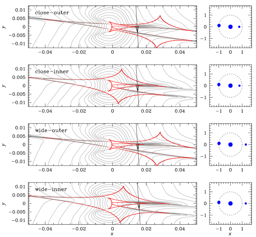
Figure 5: Lens system configurations of the 3L1S models in the population B. Notations are same as those in Fig. 4.

In the present case, population B should clearly be labeled “outer-inner” because the two values of $s_{3}$ are both less than unity. For population A, the $M_{1}$–$M_{3}$ geometry is equally far from the limits in which the outer-inner and close-wide degeneracies were derived, and so could be referred to as either. We choose to call them “outer-inner” in order to maintain the most consistent notation.

It is found that the 3L1S models can approximately describe the double-bump features of the anomaly. In Figure 2, we present the model curves and residuals of the best-fit solutions in the A (“close-outer” model) and B (“close-inner” model) populations. In Tables 1 and 2, we list the lensing parameters of the 3L1S solutions in the populations “A” and “B,” respectively, along with $\Delta\chi^{2}$ values of the model fits and the magnitude of the source according to the KMTNet scale, $I_{\rm S,KMT}$. The close-inner model of the population B solutions provides the best fit to the data, but the $\Delta\chi^{2}$ differences relative to the other models are $\Delta\chi^{2}\leq 4.2$, indicating that the degeneracies among the solutions are severe.

3.3 2L2S interpretation

The double bump feature of the anomaly may be depicted if the source is a binary and if the second source additionally approached or crossed the caustic induced by the $M_{1}$–$M_{2}$ binary lens system. We checked this possibility by conducting a model in which both the lens and source are binaries (2L2S model). In addition to the parameters of a 2L1S model, a 2L2S model requires one to include four extra parameters of $(t_{0,2},u_{0,2},\rho_{2},q_{F})$, where the subscript “2” designate the second source. We use the subscript “1” to designate the corresponding parameters related to the primary source, that is, $(t_{0,1},u_{0,1},\rho_{1})$. In the 2L2S modeling, we started with the lensing parameters of the 2L1S model describing the major bump, and tested various trajectories of the second source to check whether the minor bump could be explained by the second source.

From the 2L2S modeling, we found two solutions that could depict the double-bump feature of the anomaly. The two solutions were found from the two sets of the initial lensing parameters adopted from the close and wide 2L1S solutions, and we designate the individual solutions with $s<1.0$ and $s>1.0$ as the “close” and “wide” solutions, respectively. The lensing parameters and $\chi^{2}$ values of the two 2L2S solutions are listed in Table 3, and the corresponding lens system configurations are shown in Figure 6. It is found that the close model yields a better fit than the wide model, but the $\chi^{2}$ difference between the models, $\Delta\chi^{2}=0.2$, is very small. The model curve and the residual of the close solution are shown in Figure 2. According to the lensing configurations, both the major and minor bumps of the anomaly were produced by the successive crossings of the binary source stars over the central caustic induced by a planetary companion to the lens. The flux from the second source, which trailed the first source and approached the caustic more closely than the primary source, comprises $\sim 17\%$ of the $I$-band flux from the first source. From the comparison of the $\chi^{2}$ values with those of the 3L1S solutions, it is found that the 2L2S solutions yield a better fit than the 3L1S solutions with $\Delta\chi^{2}=[11.1$–15.3].

Table 3: 2L2S lensing parameters

Parameter	Close	Wide
$\chi^{2}$	$624.9$	$625.1$
$t_{0,1}$ (HJD$\prime$)	$9421.518\pm 0.005$	$9421.517\pm 0.004$
$u_{0,1}$	$0.016\pm 0.002$	$0.015\pm 0.002$
$t_{0,2}$ (HJD$\prime$)	$9421.669\pm 0.009$	$9421.667\pm 0.008$
$u_{0,2}$	$0.012\pm 0.004$	$0.012\pm 0.003$
$t_{\rm E}$ (days)	$22.61\pm 2.21$	$23.264\pm 2.21$
$s$	$0.795\pm 0.018$	$1.297\pm 0.029$
$q$ ($10^{-3}$)	$1.46\pm 0.29$	$1.57\pm 0.25$
$\alpha$ (rad)	$4.648\pm 0.014$	$4.643\pm 0.013$
$\rho_{1}$ ($10^{-3}$)	$3.12\pm 0.33$	$2.98\pm 0.30$
$\rho_{2}$ ($10^{-3}$)	$1.70\pm 0.64$	$1.68\pm 0.61$
$q_{F}$	$0.17\pm 0.05$	$0.17\pm 0.05$
$I_{\rm S,KMT}$ (mag)	$21.77\pm 0.12$	$21.80\pm 0.10$

According to the static 2L2S solutions, the separation between the two source stars at the time of the anomaly, $\Delta u=\{[(t_{0,1}-t_{0,2})/t_{\rm E}]^{2}+(u_{0,1}-u_{0,2})^{2}\}^{1/2}\sim 6.7\times 10^{-3}$, is very small. Assuming that this corresponds to the semi-major axis of the source orbit, that is, $a\sim\Delta uD_{\rm S}\theta_{\rm E}\sim 0.02$ AU, and the masses of the binary source stars are $M_{S_{1}}=1\leavevmode\nobreak\ M_{\odot}$ and $M_{S_{2}}=0.5\leavevmode\nobreak\ M_{\odot}$, the orbital period of the binary source is $P=[(a/{\rm AU})^{3}/(M_{S}/M_{\odot})]^{1/2}\sim 1$ day, where $M_{S}=M_{S_{1}}+M_{S_{2}}$. Because this orbital period is of the same order as the duration of the anomaly, the orbital motion of the binary source may be important to the binary-source modeling. Although it would be difficult to define the orbital lensing parameters based on the handful of data points covering the short-term anomaly, we conducted an additional modeling considering the source orbital motion to check whether the fit further improves with the consideration of the source orbital motion. From the modeling conducted under the assumption of a simplified face-on circular orbit, it is found that the fit improves by $\Delta\chi^{2}\sim 3.2$ with respect to the static model, making the gap between the 2L2S and 3L1S solutions wider, into $\Delta\chi^{2}=[14.3$–18.5]. The orbital 2L2S model and its residual are shown in Figure 2.

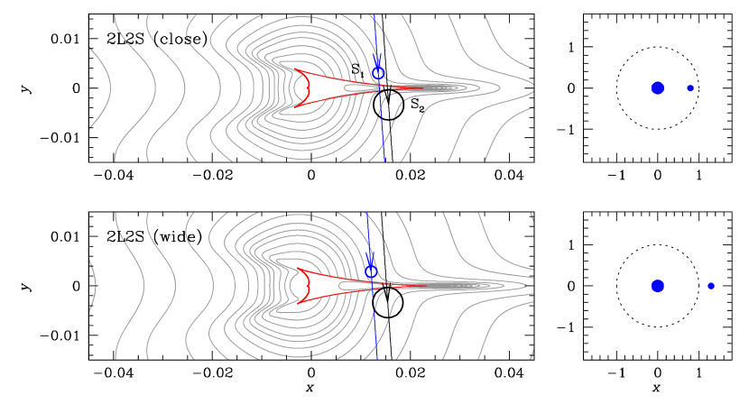
Figure 6: Lens system configurations of the close (upper panel) and wide (lower panel) 2L2S solutions. Notations are same as those in Fig. 4, except that there are two lens masses and two source trajectories. The source trajectories of the first and second source stars are marked by $S_{1}$ and $S_{2}$, respectively. The empty circles on the source trajectories represent the source positions at a certain epoch, and the sizes of the circles are scaled to the caustic size.

As is discussed in the following section, the Einstein radii derived independently from the two stars of the binary source result in consistent values. Together with the better fit, we conclude that the single-planet binary-source 2L2S interpretation of the anomaly is more plausible than the multi-planet 3L1S interpretation. According to the 2L2S interpretation, KMT-2021-BLG-1898 is the fifth binary-lensing event occurring on a binary stellar system, following MOA-2010-BLG-117 (Bennett et al., 2018), OGLE-2016-BLG-1003 (Jung et al., 2017), KMT-2018-BLG-1743 (Han et al., 2021a), and KMT-2019-BLG-0797 (Han et al., 2021b). For three of these events (MOA-2010-BLG-117, KMT-2018-BLG-1743, and KMT-2021-BLG-1898), the lenses are planetary systems.

4 Source stars and Einstein radius

We specify the source not only to fully characterize the event but also to measure the angular Einstein radius. The source was specified by measuring its color and magnitude. According to the routine procedure, the first step for this specification is measuring the source magnitudes in two passbands, $I$ and $V$ bands in our case, from the regression of the photometric data to the lensing model. For KMT-2021-BLG-1898, the $I$-band source magnitude was precisely measured, but a reliable measurement of the $V$-band magnitude was difficult because the quality of the $V$-band data was not good due to the heavy extinction toward the field. We, therefore, estimated the source color by interpolating it from the main-sequence (MS) branch of stars in the CMD constructed from the Hubble Space Telescope (HST) observations (Holtzman et al., 1998).

The detailed procedure of specifying the source type is as follows. First, we estimated the combined $I$-band source flux, $F_{S,I}=F_{S_{1},I}+F_{S_{2},I}$, from the regression of the $I$-band data processed using the pyDIA code to the model. Here $F_{S_{1},I}$ and $F_{S_{2},I}$ represent the $I$-band flux values from the primary and secondary source stars, respectively. With the flux ratio $q_{F,I}$ between the two source stars estimated from the modeling, we then estimated the flux values of the individual source stars as

$$F_{S_{1},I}=\left({1\over 1+q_{F,I}}\right)F_{S,I};\qquad F_{S_{2},I}=\left({q_{F,I}\over 1+q_{F,I}}\right)F_{S,I}.$$ (5)

Second, we made a combined CMD by aligning the HST CMD and that constructed with the pyDIA photometry of the KMTC data set using the centroids of red giant clumps (RGCs) in the individual CMDs. We then estimate the colors of $S_{1}$ and $S_{2}$ by interpolating them from the MS branch on the HST CMD corresponding to the $I$-band magnitudes of $S_{1}$ and $S_{2}$.

It is found that the two source stars are 3.20 mag and 5.43 mag fainter than the RGC centroid. With the known values of the extinction and reddening-corrected (de-reddened) color and magnitude, $(V-I,I)_{\rm RGC}=(1.06,14.39)$ (Bensby et al., 2013; Nataf et al., 2013), for the RGC centroid, we estimate that the de-reddened colors and magnitudes of the source stars are

$$(V-I,I)_{0,S_{1}}=(0.75\pm 0.07,17.59\pm 0.05)$$ (6)

for the primary source, and

$$(V-I,I)_{0,S_{2}}=(1.02\pm 0.10,19.81\pm 0.40)$$ (7)

for the secondary source. Here, the error of the $I$-band magnitude for $S_{2}$ was estimated from the error propagation of the magnitude uncertainty of $S_{1}$ together with the uncertainty of $q_{F,I}$ measurement. For each star, we estimated the color directly from the median color of stars with the same offset from the clump on the HST CMD based on images of Baade’s window. We derived the error bars from the scatter in $(V-I)$ at fixed offset by first taking account of the photometric measurement errors that were described by Holtzman et al. (1998). Figure 7 shows the locations of $S_{1}$ and $S_{2}$ on the HST CMD. The estimated colors and magnitudes indicate that the primary source is a turnoff star or a subgiant with a G spectral type, and the secondary source is a mid K-type dwarf. Also marked in the CMD is the location of the blend, which is fainter than the RGC centroid by 1.25 mag in the $I$ band. As was in the case of the source, the color of the blend could not be measured directly from the photometric data due to the poor $V$-band data. We, therefore, estimate the blend color as the median value of the giant branch corresponding to the $I$-band magnitude difference from the RGC centroid.

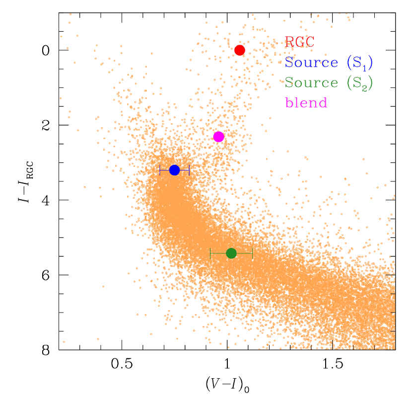
Figure 7: Locations of the primary ($S_{1}$) and secondary ($S_{2}$) source stars with respect to the centroid of red giant clump (RGC) in the color-magnitude diagram constructed from the Hubble Space Telescope observations. The abscissa represents the de-reddened color $(V-I)_{0}$, while the ordinate denotes the $I$-band magnitude difference with respect to that of the RGC centroid.

With the specified source type, we estimate the angular Einstein radius by

$$\theta_{\rm E}={\theta_{*,S_{1}}\over\rho_{1}}$$ (8)

where $\theta_{*,S_{1}}$ represents the angular radius of $S_{1}$. For the estimation of the angular source size from the measured color, we first convert $V-I$ color into $V-K$ using the color-color relation of Bessell & Brett (1988), and then interpolate $\theta_{*,S_{1}}$ from the $(V-K)$–$\theta_{*}$ relation of Kervella et al. (2004). This yields the angular radius of the primary source of

$$\theta_{*,S_{1}}=0.99\pm 0.11\leavevmode\nobreak\ \mu{\rm as},$$ (9)

and the angular Einstein radius of

$$\theta_{\rm E}=0.32\pm 0.05\leavevmode\nobreak\ {\rm mas}.$$ (10)

The relative lens-source proper motion is estimated from the combination of the Einstein radius and event time scale as

$$\mu={\theta_{\rm E}\over t_{\rm E}}=5.11\pm 0.47\leavevmode\nobreak\ {\rm mas}\leavevmode\nobreak\ {\rm yr}^{-1}.$$ (11)

The validity of the 2L2S interpretation is further supported by the fact that the angular Einstein radii derived independently from the two stars of the binary source result in consistent values. To demonstrate this, we estimated two values of $\theta_{\rm E}$: one derived from the source type and $\rho_{1}$ of the primary source, $\theta_{\rm E,1}$, and the other from those of the secondary source, $\theta_{\rm E,2}$. Figure 8 shows the scatter plots of MCMC points on the $\rho_{1}$–$\rho_{2}$ (left panel) and $\theta_{\rm E,1}$–$\theta_{\rm E,2}$ (right panel) planes. We note that the $\theta_{\rm E,1}$–$\theta_{\rm E,2}$ scatter plot is elongated along the ordinate direction due to the large uncertainty of $\rho_{2}$. The plots shows that the Einstein radii estimated from $S_{1}$ and $S_{2}$ result in consistent values, which is $\theta_{\rm E}\sim 0.3$ mas, and this further supports the 2L2S model in addition to its better fit than fit of the 3L1S interpretation.

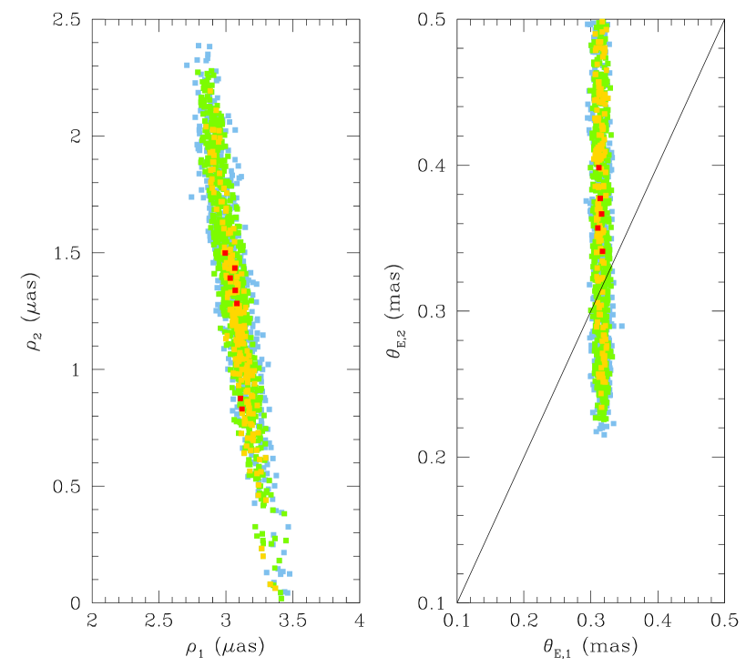
Figure 8: Scatter plot of points in the MCMC chain on the $\rho_{1}$–$\rho_{2}$ (left panel) and $\theta_{\rm E,1}$–$\theta_{\rm E,2}$ (right panel) planes obtained from the 2L2S modeling. The color coding is the same as that in Fig. 2 except that $n=1$. The diagonal line in the right panel represents the relation $\theta_{\rm E,1}=\theta_{\rm E,2}$.

Table 4: Physical lens parameters

Quantity	Close	Wide
$M_{\rm host}$ ($M_{\odot}$)	$0.48^{+0.33}_{-0.26}$	$\leftarrow$
$M_{\rm planet}$ ($M_{\rm J}$)	$0.73^{+0.50}_{-0.40}$	$0.79^{+0.54}_{-0.43}$
$D_{\rm L}$ (kpc)	$6.9^{+0.9}_{-1.3}$	$\leftarrow$
$a_{\perp}$ (AU)	$1.9^{+0.3}_{-0.3}$	$3.0^{+0.4}_{-0.6}$

5 Physical parameters of the planetary system

The lensing observables that can constrain the physical lens parameters of the mass, $M$, and distance, $D_{\rm L}$, include the event time scale $t_{\rm E}$, Einstein radius $\theta_{\rm E}$, and microlens parallax $\pi_{\rm E}$. With the measurements of all these observables, the physical parameters can be uniquely determined as

$$M={\theta_{\rm E}\over\kappa\pi_{\rm E}};\qquad D_{\rm L}={{\rm AU}\over\pi_{\rm E}\theta_{\rm E}+\pi_{\rm S}},$$ (12)

where $\kappa=4G/(c^{2}{\rm AU})$, $\pi_{\rm S}={\rm AU}/D_{\rm S}$ is the trigonometric parallax of the source lying at a distance $D_{\rm S}$ (Gould, 2000). For KMT-2021-BLG-1898, the observables of $t_{\rm E}$ and $\theta_{\rm E}$ were measured from the modeling of the light curve. However, the microlens parallax $\pi_{\rm E}$, which can be measured from the subtle deviations in the lensing light curve from the symmetric form induced by the positional change of the source caused by the orbital motion of Earth around the Sun (Gould, 1992), could not be securely measured due to the relatively short time scale, $t_{\rm E}\sim 23$ days, of the event together with the low precision of the photometric data. Although $M$ and $D_{\rm L}$ cannot be uniquely determined, one can still constrain them using the other observables, which are related to the physical parameters by

$$t_{\rm E}={\theta_{\rm E}\over\mu};\qquad\theta_{\rm E}=(\kappa M\pi_{\rm rel})^{1/2},$$ (13)

where $\pi_{\rm rel}={\rm AU}(D_{\rm L}^{-1}-D_{\rm S}^{-1})$ is the relative lens-source parallax.

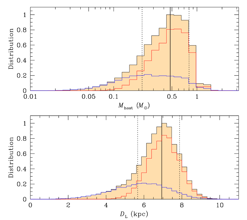
Figure 9: Bayesian posteriors of the host mass (upper panel) and distance (lower panel) to the planetary system. In each panel, the red and blue curves represent the contributions by the bulge and disk lens populations, respectively, and the black curve is the sum of the two populations. The solid vertical line indicates the median of the distribution, and the two dotted vertical lines represent the 1$\sigma$ range of the distribution.

The lens parameters were estimated from a Bayesian analysis conducted with the use of the measured observables $t_{\rm E}$ and $\theta_{\rm E}$. In the first step of the Bayesian analysis, we conducted a Monte Carlo simulation to produce a large number ($2\times 10^{6}$) of artificial lensing events. The simulation was done using a prior Galactic model defining the locations, motions, and masses of Galactic objects. We used the Galactic model of Jung et al. (2021) in the simulation. The model was constructed using the Robin et al. (2003) and Han & Gould (2003) models for the physical distributions of disk and bulge objects, respectively, Jung et al. (2021) and Han & Gould (1995) models for the dynamical distributions of the disk and bulge objects, respectively, and Jung et al. (2018) model for the mass function for the lenses. In the second step, we constructed the posterior distributions of the physical lens parameters of $M$ and $D_{\rm L}$ for the simulated events with event time scales and angular Einstein radii that were consistent with observed values of $t_{\rm E}$ and $\theta_{\rm E}$. With the constructed distributions, we present the median values as the representative values of the physical parameters, and set the 16% and 84% of the distributions as the lower and upper limits of the 1$\sigma$ ranges.

Figure 9 shows the posterior distributions of the mass of the planet host and distance to the planetary system constructed from the Bayesian analysis. In Table 4, we list the estimated parameters of the host mass, $M_{\rm host}$, planet mass, $M_{\rm planet}$, distance, and projected separation between the planet and host, $a_{\perp}=sD_{\rm L}\theta_{\rm E}$, corresponding to the close and wide solutions. It turns out that the lens is a planetary system in which a planet with a mass of $\sim 0.7$–0.8 $M_{\rm J}$ orbits an early M dwarf host with a mass of $\sim 0.5\leavevmode\nobreak\ M_{\odot}$, and the projected planet-host separation is $\sim 1.5$ AU and $\sim 2.5$ AU according to the close and wide solutions, respectively. The relative probabilities for the lens to be in the disk and bulge are 32% and 68%, respectively, and thus the planetary system is more likely to be in the bulge. According to the estimated mass and distance, the $I$-band magnitude of the planet host is $I\sim M_{I}+5\log D_{\rm L}-5+A_{I}\sim 25.5$, where $M_{I}\sim 7.7$ is the $I$-band absolute magnitude corresponding to the mass. Due to the faintness, the lens does not appear in the list of the Gaia Early Data Release 3 (Gaia Collaboration, 2021).

6 Conclusion

We analyzed the microlensing event KMT-2021-BLG-1898, for which the lensing light curve exhibited a short-term anomaly near the peak. It was found that the anomaly with double-bump features could not be explained by the usual binary-lens or binary-source interpretations. In order to reveal the nature of the anomaly, we conducted modeling of the light curve under various sophisticated models with the inclusion of additional lens or source component.

We found that the anomaly was best explained by a model, in which both the lens and source are binaries. For this model, the lens is a planetary system with a planet/host mass ratio, and the source is a binary composed of a turn-off or a subgiant star and a mid K dwarf. The double-bump feature of the anomaly could also be described by a triple-lens model, in which the lens is a planetary system containing two planets. Among the two models, the 2L2S model was favored over the 3L1S model not only because it yields a better fit to the data but also the Einstein radii derived independently from the two stars of the binary source result in consistent values. According to the 2L2S interpretation, KMT-2021-BLG-1898 is the fifth event in which both the lens and source are binaries, and the third 2L2S case in which the lens is a planetary system. degeneracy in the planet-host separation.

From a Bayesian analysis based on the observables of the event, we estimated that the planet has a mass of $\sim 0.7$–0.8 $M_{\rm J}$, and it orbits an early M dwarf host with a mass of $\sim 0.5\leavevmode\nobreak\ M_{\odot}$. The projected planet-host separation is $\sim 1.5$ AU and $\sim 2.5$ AU according to the close and wide solutions, respectively.