Numerical Computation of Partial Differential Equations by Hidden-Layer Concatenated Extreme Learning Machine

Abstract

The extreme learning machine (ELM) method can yield highly accurate solutions to linear/nonlinear partial differential equations (PDEs), but requires the last hidden layer of the neural network to be wide to achieve a high accuracy. If the last hidden layer is narrow, the accuracy of the existing ELM method will be poor, irrespective of the rest of the network configuration. In this paper we present a modified ELM method, termed HLConcELM (hidden-layer concatenated ELM), to overcome the above drawback of the conventional ELM method. The HLConcELM method can produce highly accurate solutions to linear/nonlinear PDEs when the last hidden layer of the network is narrow and when it is wide. The new method is based on a type of modified feedforward neural networks (FNN), termed HLConcFNN (hidden-layer concatenated FNN), which incorporates a logical concatenation of the hidden layers in the network and exposes all the hidden nodes to the output-layer nodes. HLConcFNNs have the interesting property that, given a network architecture, when additional hidden layers are appended to the network or when extra nodes are added to the existing hidden layers the representation capacity of the HLConcFNN associated with the new architecture is guaranteed to be not smaller than that of the original network architecture. Here representation capacity refers to the set of all functions that can be exactly represented by the neural network of a given architecture. We present ample benchmark tests with linear/nonlinear PDEs to demonstrate the computational accuracy and performance of the HLConcELM method and the superiority of this method to the conventional ELM from previous works.

Keywords: extreme learning machine, hidden layer concatenation, random weight neural networks, least squares, scientific machine learning, random basis

1 Introduction

This work continues and extends our recent studies DongL2021 ; DongL2021bip ; DongY2021 of a type of random-weight neural networks, the so-called extreme learning machines (ELMs) HuangZS2006 , for scientific computing and in particular for computational partial differential equations (PDEs). Specifically, we would like to address the following question:

• Can ELM achieve a high accuracy for solving linear/nonlinear PDEs on network architectures with a narrow last hidden layer?

For the existing ELM method DongL2021 ; DongL2021bip ; DongY2021 (referred to as the conventional ELM hereafter), the answer to this question is negative. The goal of this paper is to introduce a modified method, referred to as the hidden-layer concatenated ELM (HLConcELM), to overcome this drawback of the conventional ELM and provide a positive answer to the above question.

Exploiting randomization in neural networks has a long history ScardapaneW2017 . Turing’s un-organized machine Webster2012 and Rosenblatt’s perceptron Rosenblatt1958 in the 1950s are early examples of randomized neural networks. After a hiatus of several decades, there has been a strong revival of methods based on random-weight neural networks, starting in the 1990s SuganthanK2021 . In recent years randomization based neural networks have attracted a growing interest in a variety of areas ScardapaneW2017 ; FreireRB2020 .

Since it is enormously costly and hard to optimize the entire set of adjustable parameters in the neural network, it seems advisable if one randomly assigns and fixes a subset of the network’s parameters so that the ensuing optimization task of network training can be simpler, and ideally linear, without severely compromising the network’s achievable approximation capability. This philosophy underlies the randomization of neural networks. When applied to feedforward or recurrent neural networks, randomization leads to techniques such as the random vector functional link (RVFL) networks PaoT1992 ; PaoPS1994 ; IgelnikP1995 , the extreme learning machine HuangZS2004 ; HuangZS2006 ; HuangCS2006 , the echo-state network JaegerLPS2007 ; LukoseviciusJ2009 , the no-propagation network WidrowGKP2013 , and the liquid state machine MaasM2004 . The random-weight neural networks (with a single hidden layer) are universal function approximators. The universal approximation property of such networks has been studied in IgelnikP1995 ; LiCIP1997 ; HuangCS2006 ; NeedellNSS2020 . The theoretical results of IgelnikP1995 ; HuangCS2006 ; NeedellNSS2020 establish that a single hidden-layer feedforward neural network having random but fixed (not trained) hidden nodes can approximate any continuous function to any desired degree of accuracy, provided that the number of hidden nodes is sufficiently large. The expected rate of convergence in the approximation of Lipschitz continuous functions is given in IgelnikP1995 ; RahimiR2008 ; NeedellNSS2020 .

ELM was originally developed in HuangZS2004 ; HuangZS2006 for single hidden-layer feedforward neural networks for linear classification/regression problems. It has since undergone a dramatic growth and found widespread applications in a variety of areas (see e.g. the reviews of HuangHSY2015 ; Alabaetal2019 and the references therein). The method is based on two strategies: (i) randomly assigned but fixed (not trainable) hidden-layer coefficients, and (ii) trainable linear output-layer coefficients computed by a linear least squares method or by using the pseudoinverse (Moore-Penrose inverse) of the coefficient matrix VermaM1994 ; PaoPS1994 ; BraakeS1995 ; GuoCS1995 .

While ELM emerged nearly two decades ago, the investigation of this technique for the numerical solution of differential equations has appeared only quite recently, alongside the proliferation of deep neural network (DNN) based PDE solvers in the past few years (see e.g. Karniadakisetal2021 ; SirignanoS2018 ; RaissiPK2019 ; EY2018 ; WinovichRL2019 ; HeX2019 ; CyrGPPT2020 ; JagtapKK2020 ; WangL2020 ; WanW2020 ; DongN2021 ; LuMMK2021 ; TangWL2021 ; KrishnapriyanGZKM2021 ; WangYP2022 , among many others). In YangHL2018 ; Sunetal2019 ; LiuXWL2020 ; LiuHWC2021 the ELM technique has been used for solving linear ordinary or partial differential equations (ODEs/PDEs) with single hidden-layer feedforward neural networks, in which certain polynomials (e.g. Legendre, Chebyshev, or Bernstein polynomials) serve as the activation function. In PanghalK2020 the ELM algorithm is used for solving linear ODEs and PDEs on neural networks with a single hidden layer, in which the Moore-Penrose inverse of the coefficient matrix has been used. In DwivediS2020 a physics-informed ELM method is proposed for solving linear PDEs by combining the physics-informed neural network and the ELM idea. The neural network consists of a single hidden layer, and the Moore-Penrose inverse is employed to solve the resultant linear system. Interestingly, the authors set the number of hidden nodes to be equal to the total number of conditions in the problem. A solution strategy based on the normal equation associated with the linear system is studied in DwivediS2022 .

The ELM approach is extended to the numerical solution of nonlinear PDEs in DongL2021 on local or global feedforward neural networks with a single or multiple hidden layers. A nonlinear least squares method with perturbations (NLLSQ-perturb) and a Newton-linear least squares (Newton-LLSQ) method are developed for solving the resultant nonlinear algebraic system for the output-layer coefficients of the ELM neural network. The NLLSQ-perturb algorithm therein takes advantage of the nonlinear least squares routine from the scipy library, which implements a Gauss-Newton type method combined with a trust-region strategy. A block time marching (BTM) scheme is proposed in DongL2021 for long-time dynamic simulations of linear and nonlinear PDE problems, in which the temporal dimension (if large) is divided into a number of windows (called time blocks) and the PDE problem is solved on the time blocks individually and successively. More importantly, a systematic comparison of the accuracy and the computational cost (network training time) between the ELM method and two state-of-the-art deep neural network (DNN) based PDE solvers, the deep Galerkin method (DGM) SirignanoS2018 and the physics-informed neural network (PINN) method RaissiPK2019 , has been conducted in DongL2021 , as well as a systematic comparison between ELM and the classical finite element method (FEM). The comparisons show that the ELM method far outperforms DGM and PINN in terms of the accuracy and the computational cost, and that ELM is on par with the classical FEM in computational performance and outperforms the FEM as the problem size becomes larger. In DongL2021 the hidden-layer coefficients are set to uniform random values generated on $[-R_{m},R_{m}]$, where $R_{m}$ is a user-prescribed constant. The results of DongL2021 show that the $R_{m}$ value has a strong influence on the numerical accuracy of the ELM results and that the best accuracy is associated with a range of moderate $R_{m}$ values for a given problem. This is consistent with the observation for classification problems ZhangS2016 .

A number of further developments of the ELM technique for solving linear and nonlinear PDEs appeared recently; see e.g. DongL2021bip ; CalabroFS2021 ; GalarisFCSS2021 ; DongY2021 ; FabianiCRS2021 , among others. In order to address the influence of random initialization of the hidden-layer coefficients on the ELM accuracy, a modified batch intrinsic plasticity (modBIP) method is developed in DongL2021bip for pre-training the random coefficients in the ELM network. This method, together with ELM, is applied to a number of linear and nonlinear PDEs. The accuracy of the combined modBIP/ELM method has been shown to be insensitive to the random initializations of the hidden-layer coefficients. In CalabroFS2021 the authors present a method for solving one-dimensional linear elliptic PDEs based on ELM with single hidden-layer feedforward neural networks and the sigmoid activation function. The random parameters in the activation function are set based on the location of the domain of interest and the function derivative information. In GalarisFCSS2021 the authors present a method based on randomized neural networks with a single hidden layer for solving stiff ODEs. The time integration therein appears similar to the block time marching strategy DongL2021 but with an adaptation on the time block sizes. It is observed that the presented method is advantageous over the stiff ODE solvers from MatLab. Noting the influence of the maximum random-coefficient magnitude (i.e. the $R_{m}$ constant) on the ELM accuracy as shown by DongL2021 , in DongY2021 we have presented a method for computing the optimal $R_{m}$ in ELM based on the differential evolution algorithm, as well as an improved implementation for computing the differential operators of the last hidden-layer data. These improvements significantly enhance the ELM computational performance and dramatically reduce its network training time as compared with that of DongL2021 . The improved ELM method is compared systematically with the traditional second-order and high-order finite element methods for solving a number of linear and nonlinear PDEs in DongY2021 . The improved ELM far outperforms the second-order FEM. For smaller problem sizes it is comparable to the high-order FEM in performance, and for larger problem sizes the improved ELM outperforms the high-order FEM markedly. Here, by “outperform” we mean that one method achieves a better accuracy under the same computational cost or incurs a lower computational cost to achieve the same accuracy. In FabianiCRS2021 an ELM method is presented for the numerical solution of stationary nonlinear PDEs based on the sigmoid and radial basis activation functions. The authors observe that the ELM method exhibits a better accuracy than the finite difference and the finite element method. Another recent development related to ELM is DongY2022 , in which a method based on the variable projection strategy is proposed for solving linear and nonlinear PDEs with artificial neural networks. For linear PDEs, the neural-network representation of the PDE solution leads to a separable nonlinear least squares problem, which is then reformulated to eliminate the output-layer coefficients, leading to a reduced problem about the hidden-layer coefficients only. The reduced problem is solved first by the nonlinear least squares method to determine the hidden-layer coefficients, and the output-layer coefficients are then computed by the linear least squares method DongY2022 . For nonlinear PDEs, the problem is first linearized by the Newton’s method with a particular linearization form, and the linearized system is solved by the variable projection framework together with neural networks. The ELM method can be considered as a special case of the variable projection, i.e. with zero iteration when solving the reduced problem for the hidden-layer coefficients DongY2022 . It is shown in DongY2022 that the variable projection method exhibits an accuracy significantly superior to the ELM under identical conditions and network configurations.

As has been shown in previous works DongL2021 ; DongL2021bip ; DongY2021 , ELM can produce highly accurate results for solving linear and nonlinear PDEs. For smooth field solutions the ELM errors decrease exponentially as the number of training data points or the number of training parameters in the neural network increases, and the errors can reach a level close to the machine zero when the number of degrees of freedom becomes large. To achieve a high accuracy, however, the existing ELM method requires the number of nodes in the last hidden layer of the neural network to be sufficiently large DongL2021 . Therefore, the ELM network usually has a wide hidden layer in the case of a shallow neural network, or a wide last hidden layer in the case of deeper neural networks. If the last hidden layer contains only a small number of nodes, the results computed with the existing (conventional) ELM will tend to be poor in accuracy, regardless of the configuration with the rest of the network.

In this paper, we focus on feedforward neural networks (FNNs) with multiple hidden layers, and present a modified ELM method (termed HLConcELM) for solving linear/nonlinear PDEs to overcome the above drawback associated with the conventional ELM method. The HLConcELM method can produce accurate solutions to linear/nonlinear PDEs when the last hidden layer of the network is narrow, and when the last hidden layer is wide.

The new method is based on a type of modified feedforward neural networks, referred to as hidden-layer concatenated FNN (or HLConcFNN) herein, which incorporates a logical concatenation of the hidden layers so that all the hidden nodes are exposed to and connected with the nodes in the output layer (see Section 2 for details). The HLConcFNNs have the interesting property that, given a network architecture, when additional hidden layers are appended to the neural network or when extra nodes are added to the existing hidden layers, the representation capacity of the HLConcFNN associated with the new architecture is guaranteed to be not smaller than that associated with the original network architecture. Here by representation compacity we refer to the set of all functions that can be exactly represented by the neural network (see Section 2 the definition). In contrast, conventional FNNs do not have a parallel property when additional hidden layers are appended to the network.

The HLConcELM is attained by setting (and fixing) the weight/bias coefficients in the hidden layers of the HLConcFNN to random values and allowing the connection coefficients between all the hidden nodes and the output nodes to be adjustable (trainable). More specifically, given a network architecture with $L$ hidden layers, we set the weight/bias coefficients of the $l$-th ($1\leqslant l\leqslant L$) hidden layer to uniform random values generated on the interval $[-R_{l},R_{l}]$, where $R_{l}$ is a constant. The vector of $R_{l}$ constants (referred to as the hidden magnitude vector herein), $\mathbf{R}=(R_{1},R_{2},\dots,R_{L})$, influences the accuracy of HLConcELM, and in this paper we determine the optimal $\mathbf{R}$ using the method from DongY2021 based on the differential evolution algorithm. HLConcELMs partly inherit the non-decreasing representation capacity property of HLConcFNNs. For example, given a network architecture, when extra hidden layers are appended to the network, the representation capacity of the HLConcELM associated with the new architecture will not be smaller than that associated with the original architecture, provided that the random hidden-layer coefficients for the new architecture are assigned in an appropriate fashion. On the other hand, when extra nodes are added to the existing hidden layers, HLConcELMs in general do not have a non-decreasing property with regard to its representation capacity, because of the randomly assigned hidden-layer coefficients.

The exploration of neural-network architecture has been actively pursued in machine learning research, and the connectivity patterns are the focus of a number of research efforts. Neural networks incorporating shortcut connections (concatenations) between the input nodes, the hidden nodes, and the output nodes are explored in e.g. HuangLMW2018 ; WilamowskiY2010 ; CortesGKMY2016 ; KatuwalST2019 (among others). The hidden-layer concatenated neural network adopted in the current paper can be considered in spirit as a simplification of the connection patterns in the DenseNet HuangLMW2018 architecture, and it is similar to the deep RVFL architecture of KatuwalST2019 but without the connection between the input nodes and the output nodes. We note that these previous works are for image and data classification problems, while the current work focuses on scientific computing and in particular the numerical solutions of partial differential equations.

We present extensive numerical experiments with several linear and nonlinear PDEs to test the performance of the HLConcELM method and compare the current method with the conventional ELM method. These benchmark tests demonstrate unequivocally that HLConcELM can achieve highly accurate results when the last hidden layer in the neural network is narrow or wide, and that it is much superior in accuracy to the conventional ELM method. The implementation of the current method is in Python and employs the Tensorflow (www.tensorflow.org), Keras (keras.io), and the scipy libraries. All the benchmark tests are performed on a MAC computer (3.2GHz Intel Core i5 CPU, 24GB memory) in the authors’ institution.

The contribution of this work lies in two aspects. The main contribution lies in the HLConcELM method for solving linear and nonlinear PDEs. The other aspect is with regard to the non-decreasing representation capacity of HLConcFNNs when additional hidden layers are appended to an existing network architecture. To the best the authors’ knowledge, this property seems unknown to the community so far. Bringing this property into collective consciousness can be another contribution of this paper.

The rest of this paper is organized as follows. In Section 2 we discuss the structures of HLConcFNNs and HLConcELMs, as well as their non-decreasing representation capacity property when additional hidden layers are appended to an existing architecture. We then develop the algorithm for solving linear and nonlinear PDEs employing the HLConcELM architecture. In Section 3 we present extensive benchmark examples to test the current HLConcELM method and compare its performance with that of the conventional ELM. Section 4 concludes the presentation with several further comments about the presented method. In the Appendix we include constructive proofs to some theorems from Section 2 concerning the representation capacity of HLConcFNNs.

2 Hidden-Layer Concatenated Extreme Learning Machine

2.1 Conventional ELM and Drawback

The ELM method with feedforward neural networks (FNN) for solving linear/nonlinear PDEs has been described in e.g. DongL2021 ; DongL2021bip ; DongY2021 . Figure 1(a) illustrates such a network containing three hidden layers. From layer to layer, the arrow in the sketch represents the usual FNN logic, an affine transform followed by a function composition with an activation function GoodfellowBC2016 . For ELM we require that no activation function be applied to the output layer and that the output layer contain no bias. So the output layer is linear and has zero bias. This requirement is adopted throughout this paper.

As discussed in DongL2021 , we pre-set the weight/bias coefficients in all the hidden layers to random values and fix these values once they are set. Only the weight coefficients of the output layer are trainable. The hidden-layer coefficients in the neural network are not trainable with ELM.

To solve a given linear or nonlinear PDE with ELM, we first enforce the PDE and the associated boundary/initial conditions on a set of collocation points in the domain or on the appropriate domain boundaries. This gives rise to a linear least squares problem for linear PDEs, or a nonlinear least squares problem for nonlinear PDEs, about the output-layer coefficients (trainable parameters) of the neural network DongL2021 . We solve this least squares problem for the output-layer coefficients by a linear least squares method for linear PDEs and by a nonlinear least squares method for nonlinear PDEs DongL2021 .

ELM can produce highly accurate solutions to PDEs. In particular, for smooth solutions its errors decrease exponentially as the number of collocation points or the number of trainable parameters (the number of nodes in the last hidden layer) increases DongL2021 ; DongL2021bip . In addition, it has a low computational cost (network training time) DongL2021 ; DongY2021 .

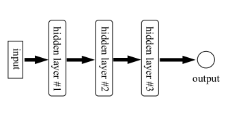
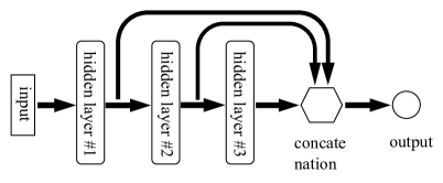
(a)  (b)

Figure 1: Illustration of neural network structure (with $3$ hidden layers): (a) conventional FNN, and (b) hidden-layer concatenated FNN (HLConcFNN). In HLConcFNN all the hidden nodes are exposed to the output nodes, while in conventional FNN only the last hidden-layer nodes are exposed to the output nodes.

Hereafter we refer to a vector or a list of positive integers as an architectural vector (denoted by $\mathbf{M}$),

$$\text{architectural vector:}\quad\mathbf{M}=[M_{0},M_{1},\dots,M_{L-1},M_{L}]$$ (1)

where $(L+1)$ is the dimension of the vector with $L\geqslant 2$, and $M_{i}$ ($0\leqslant i\leqslant L$) are positive integers. We associate a given $\mathbf{M}$ to the architecture of an FNN with $(L+1)$ layers, where $M_{i}$ ($0\leqslant i\leqslant L$) is the number of nodes in the $i$-th layer. The layer $0$ and the layer $L$ represent the input and the output layers, respectively. The layers in between are the hidden layers.

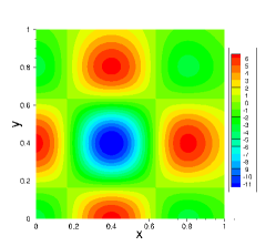
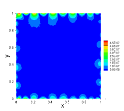
(a) (b) (c)

Figure 2: Illustration of error characteristics of conventional ELM (Poisson equation): Distributions of (a) the exact solution, (b) the ELM error obtained with the architecture $\mathbf{M}_{1}=[2,300,30,1]$, and (c) the ELM error obtained with the architecture $\mathbf{M}_{2}=[2,300,400,1]$.

Despite its high accuracy and attractive computational performance, certain aspect of the ELM method is less appealing and remains to be improved. One particular aspect in this regard concerns the size of the last hidden layer of the ELM network. ELM requires the last hidden layer of the neural network to be wide in order to achieve a high accuracy, irrespective of the sizes of the rest of the network architecture. If the last hidden layer contains only a small number of nodes, the ELM accuracy will be poor even though the preceding hidden layers can be wide enough. This point is illustrated by Figure 2, which shows the ELM results for solving the two-dimensional (2D) Poisson equation on a unit square. Figure 2(a) shows the distribution of the exact solution. Figures 2(b) and (c) show the ELM error distributions obtained using two network architectures given by $[2,300,30,1]$ and $[2,300,400,1]$, respectively, under otherwise identical conditions. Both neural networks have the Gaussian activation function $\sigma(x)=e^{-x^{2}}$ for all the hidden nodes, and are trained on a uniform set of $21\times 21$ collocation points. The only difference between them is the size of the last hidden layer. With $400$ nodes in the last hidden layer the ELM solution is highly accurate, with the maximum error on the order $10^{-7}$ in the domain. With $30$ nodes in the last hidden layer, on the other hand, the ELM solution exhibits no accuracy at all, with the maximum error on the order of $10^{2}$, despite the fact that the first hidden layer is fairly large (containing $300$ nodes). With the existing ELM method, only the last hidden-layer nodes directly contribute to the the output of the neural network, while the nodes in the preceding hidden layers do not directly affect the network output. In other words, with the existing ELM, all the degrees of freedom provided by the nodes in the preceding hidden layers are to some extent “wasted”.

Another less desirable aspect of the existing ELM method concerns its accuracy when the depth of the neural network increases. Numerical experiments indicate that increasing the number of hidden layers in the neural network seems to generally cause the accuracy of the ELM results to deteriorate. For example, the ELM accuracy with a single hidden layer in the neural network is generally better than (or comparable to) that obtained with two hidden layers in the neural network, under otherwise identical or comparable conditions. The accuracy with two hidden layers is generally better than that with three hidden layers in the neural network. With even more hidden layers in the neural network, the ELM accuracy tends to be not as accurate as those corresponding to one, two or three hidden layers (see the discussions on page 21 of DongL2021 ).

Can one achieve a high accuracy even if the last hidden layer is narrow in the ELM network? Can we take advantage of the degrees of freedom provided by the hidden nodes in the preceding hidden layers with ELM? These are the questions we are interested in and would like to address in the current work.

The above drawback of the existing ELM method, which will be referred to as the conventional ELM hereafter, motivates the developments in what follows. We present a modified ELM method to address this issue and discuss how to use the modified method for numerical simulations of PDEs.

2.2 Modifying ELM Neural Network with Hidden-Layer Concatenation

To address the aforementioned drawback, we consider a type of modified FNNs for ELM computation. The idea of the modified network is illustrated in Figure 1(b) using three hidden layers as an example.

The main strategy here is to expose all the hidden nodes in the neural network to the output-layer nodes. Starting with a standard FNN, we incorporate a logical concatenation layer between the last hidden layer and the output layer. This logical layer concatenates the output fields of all the hidden nodes, from the first to the last hidden layers, in the original network architecture. From the logical concatenation layer to the output layer a usual affine transform, together with possibly a function composition with an activation function, is performed to attain the output fields of the overall neural network. Note that the logical concatenation layer involves no parameters.

Hereafter we refer to this type of modified neural networks as the hidden-layer concatenated FNN (HLConcFNN), and the original FNN as the base neural network. Thanks to the logical concatenation, in HLConcFNN all the hidden nodes in the base network architecture are connected with the output nodes.

One can also include the input fields in the logical concatenation layer. Numerical experiments show that, however, there is no advantage in terms of the accuracy when the input fields are included. In the current paper we do not include the input fields in the concatenation.

Let us next use a real-valued function of $d$ ($d\geqslant 1$) variables, $u(\mathbf{x})$ ($\mathbf{x}\in\Omega\subset\mathbb{R}^{d}$), represented by a HLConcFNN to illustrate some of its properties. Consider a HLConcFNN, whose base architecture is given by $\mathbf{M}$ in (1), where $M_{0}=d$ and $M_{L}=1$. The $d$ input nodes represent the $d$ components of $\mathbf{x}=(x_{1},x_{2},\dots,x_{d})$, and the single output node represents the function $u(\mathbf{x})$. Let $\sigma:\mathbb{R}\rightarrow\mathbb{R}$ denote the activation function for all the hidden nodes. As stated before, we require that no activation function be applied to the output node and that it contain no bias.

Let $\bm{\Phi}^{(i)}(\mathbf{x})=\left(\phi^{(i)}_{1},\dots,\phi^{(i)}_{M_{i}}\right)$, $1\leqslant i\leqslant L-1$, denote the $M_{i}$ output fields of the $i$-th hidden layer. The logical concatenation layer contains a total of $N_{c}(\mathbf{M})=\sum_{i=1}^{L-1}M_{i}$ logical nodes. Then we have the following expansion relation,

$$u(\mathbf{x})=\sum_{i=1}^{L-1}\sum_{j=1}^{M_{i}}\beta_{ij}\phi_{j}^{(i)}(\mathbf{x})=\sum_{i=1}^{L-1}\bm{\Phi}^{(i)}(\mathbf{x})\bm{\beta}_{i}^{T}=\bm{\Phi}(\mathbf{x})\bm{\beta}^{T},$$ (2)

where $\beta_{ij}$ ($1\leqslant i\leqslant L-1$, $1\leqslant j\leqslant M_{i}$) denotes the weight coefficient of the output layer, i.e. the connection coefficient between the output node and the $j$-th hidden node in the $i$-th hidden layer, and

$$\left\{\begin{split}&\bm{\beta}_{i}=(\beta_{i1},\beta_{i2},\dots,\beta_{iM_{i}}),\quad\bm{\beta}=(\bm{\beta}_{1},\bm{\beta}_{2},\dots,\bm{\beta}_{L-1})=(\beta_{11},\dots,\beta_{1M_{1}},\beta_{21},\dots,\beta_{L-1,M_{L-1}}),\\ &\bm{\Phi}=\left(\bm{\Phi}^{(1)},\bm{\Phi}^{(2)},\dots,\bm{\Phi}^{(L-1)}\right)=\left(\phi^{(1)}_{1},\dots,\phi^{(1)}_{M_{1}},\phi^{(2)}_{1},\dots,\phi^{(L-1)}_{M_{L-1}}\right).\end{split}\right.$$ (3)

The logic from layer $(i-1)$ to layer $i$, for $1\leqslant i\leqslant L-1$, represents an affine transform followed by a function composition with the activation function,

$$\left\{\begin{split}&\phi_{j}^{(i)}(\mathbf{x})=\sigma\left(\sum_{k=1}^{M_{i-1}}\phi^{(i-1)}_{k}(\mathbf{x})w_{kj}^{(i)}+b_{j}^{(i)}\right),\quad 1\leqslant j\leqslant M_{i},\\ &\bm{\Phi}^{(i)}(\mathbf{x})=\sigma\left(\bm{\Phi}^{(i-1)}(\mathbf{x})\mathbf{W}^{(i)}+\mathbf{b}^{(i)}\right).\end{split}\right.$$ (4)

In the above equation, the constants $w_{kj}^{(i)}$ ($1\leqslant k\leqslant M_{i-1}$, $1\leqslant j\leqslant M_{i}$) are the weights and $b_{j}^{(i)}$ ($1\leqslant j\leqslant M_{i}$) are the biases of layer $i$, and

$$\mathbf{W}^{(i)}=\begin{bmatrix}w_{kj}^{(i)}\end{bmatrix}_{M_{i-1}\times M_{i}},\quad\mathbf{b}^{(i)}=\left(b_{1}^{(i)},b_{2}^{(i)},\dots,b_{M_{i}}^{(i)}\right),\quad\mathbf{\Phi}^{(0)}(\mathbf{x})=\left(\phi_{1}^{(0)},\phi_{2}^{(0)},\dots,\phi_{M_{0}}^{(0)}\right)=\mathbf{x}.$$ (5)

Define

$$\left\{\begin{split}&\bm{\theta}^{(i)}=\text{\bf{flatten}}\left[\mathbf{W}^{(i)},\mathbf{b}^{(i)}\right],\quad 1\leqslant i\leqslant L-1,\\ &\bm{\theta}=(\bm{\theta}^{(1)},\bm{\theta}^{(2)},\dots,\bm{\theta}^{(L-1)})=(\theta_{1},\theta_{2},\dots,\theta_{N_{h}}),\end{split}\right.$$ (6)

where “flatten” denotes the operation to reshape and combine a list of matrices or vectors into a single vector, and $N_{h}(\mathbf{M})=\sum_{i=1}^{L-1}(M_{i-1}+1)M_{i}$. Here $\bm{\theta}^{(i)}$ denotes the vector of weight/bias coefficients of layer $i$ for $1\leqslant i\leqslant L-1$, $\bm{\theta}$ denotes the vector of weight/bias coefficients in all the hidden layers, and $N_{h}$ is the total number of hidden-layer coefficients in the neural network.

The output field of the neural network depends on $(\bm{\theta},\bm{\beta})$, and the output fields of each hidden layer depend on $\bm{\theta}$. To make these dependencies more explicit, we re-write equation (2) into

$$u(\bm{\theta},\bm{\beta},\mathbf{x})=\sum_{i=1}^{L-1}\sum_{j=1}^{M_{i}}\beta_{ij}\phi^{(i)}_{j}(\bm{\theta},\mathbf{x})=\sum_{i=1}^{L-1}\bm{\Phi}^{(i)}(\bm{\theta},\mathbf{x})\bm{\beta}_{i}^{T}=\bm{\Phi}(\bm{\theta},\mathbf{x})\bm{\beta}^{T},$$ (7)

where $\bm{\Phi}$, $\bm{\Phi}^{(i)}$, $\bm{\beta}_{i}$ and $\bm{\beta}$ are defined in (3).

A hidden-layer concatenated FNN is characterized by the architectural vector of the base network and the activation function. Given the architectural vector $\mathbf{M}$ and an activation function $\sigma$, let HLConcFNN$(\mathbf{M},\sigma)$ denote the associated hidden-layer concatenated neural network. For a given domain $\Omega\subset\mathbb{R}^{d}$, an architectural vector $\mathbf{M}=(M_{0},M_{1},\dots,M_{L})$ with $M_{0}=d$ and $M_{L}=1$, and an activation function $\sigma(\cdot)$, we define

$$U(\Omega,\mathbf{M},\sigma)=\left\{u(\bm{\theta},\bm{\beta},\mathbf{x})\ |\ u(\bm{\theta},\bm{\beta},\mathbf{x})\ \text{is output of HLConcFNN}(\mathbf{M},\sigma),\ \mathbf{x}\in\Omega,\ \bm{\theta}\in\mathbb{R}^{N_{h}},\ \bm{\beta}\in\mathbb{R}^{N_{c}}\right\}$$ (8)

as the collection of all the possible output fields of this HLConcFNN$(\mathbf{M},\sigma)$. Note that $U(\Omega,\mathbf{M},\sigma)$ denotes the set of all functions that can be exactly represented by this HLConcFNN$(\mathbf{M},\sigma)$ on $\Omega$. Hereafter we refer to $U(\Omega,\mathbf{M},\sigma)$ as the representation capacity of the HLConcFNN$(\mathbf{M},\sigma)$ for the domain $\Omega$.

Remark 2.1.

It should be noted that $U(\Omega,\mathbf{M},\sigma)$ as defined by (8) is a set, not a linear space, for the simple fact that it is not closed under addition because of the nonlinear parameters $\bm{\theta}$.

The HLConcFNNs have an interesting property. If one appends extra hidden layers to the network architecture, or adds nodes to any of the existing hidden layers, the representation capacity of the resultant HLConcFNN is at least as large as that of the original one. On the other hand, conventional FNNs lack such a property when additional hidden layers are appended to the architecture. Specifically, we have the following results.

Theorem 2.1.

Given an architectural vector $\mathbf{M}_{1}=(m_{0},m_{1},\dots,m_{L-1},m_{L})$ with $m_{L}=1$, define a new vector $\mathbf{M}_{2}=(m_{0},m_{1},\dots,m_{L-1},n,m_{L})$, where $n\geqslant 1$ is an integer. For a given domain $\Omega\subset\mathbb{R}^{m_{0}}$ and an activation function $\sigma(\cdot)$, the following relation holds

$$U(\Omega,\mathbf{M}_{1},\sigma)\subseteq U(\Omega,\mathbf{M}_{2},\sigma),$$ (9)

where $U$ is defined by (8).

Theorem 2.2.

Given an architectural vector $\mathbf{M}_{1}=(m_{0},m_{1},\dots,m_{L})$ with $m_{L}=1$, define a new vector $\mathbf{M}_{2}=(m_{0},m_{1},\dots,m_{s-1},m_{s}+1,m_{s+1},\dots,m_{L})$ for some $s$ ($1\leqslant s\leqslant L-1$). For a given domain $\Omega\subset\mathbb{R}^{m_{0}}$ and an activation function $\sigma(\cdot)$, the following relation holds

$$U(\Omega,\mathbf{M}_{1},\sigma)\subseteq U(\Omega,\mathbf{M}_{2},\sigma),$$ (10)

where $U$ is defined by (8).

These properties can be shown to be true by simple constructions. These constructions are straightforward and border on being trivial. Risking on the side of naivety, we still include the constructive proofs for these two theorems in an Appendix of this paper for the benefit of a skeptical reader.

It should be noted that for conventional FNNs the relation given by (10) is true, but the relation given by (9) does not hold. Relation (9) is true for HLConcFNNs thanks to the concatenation of hidden layers in such networks.

Suppose we start with a base neural network architecture $\mathbf{M}_{0}$ and generate a sequence of architectures $\mathbf{M}_{i}$ ($i\geqslant 1$), with each one obtained either by adding extra nodes to the existing hidden layers of or by appending additional hidden layers to the previous architecture. Then based on the above two theorems the HLConcFNNs associated with this sequence of architectures exhibit a hierarchical structure, in the sense that the representation capacities of this sequence of HLConcFNNs do not decrease, namely

$$U(\Omega,\mathbf{M}_{0},\sigma)\subseteq U(\Omega,\mathbf{M}_{1},\sigma)\subseteq\cdots\subseteq U(\Omega,\mathbf{M}_{n},\sigma)\subseteq\cdots.$$ (11)

If the activation function $\sigma(\cdot)$ is nonlinear, the representation capacities of this sequence of HLConcFNNs should strictly increase.

Remark 2.2.

If the number of nodes in the output layer of the HLConcFNN is more than one, the relations given by Theorems 2.1 and 2.2 about the representation capacities equally hold.

Hidden-Layer Concatenated Extreme Learning Machine (HLConcELM)

Let us next combine the hidden-layer concatenated feedforward neural networks with the idea of ELM. We adopt HLConcFNNs as the neural network for the ELM computation. We pre-set (and fix) all the weight/bias coefficients in the hidden layers (i.e. $\bm{\theta}$) of the HLConcFNN to random values, and train/compute the output-layer coefficients (i.e. $\bm{\beta}$) by a linear or nonlinear least squares method. We will refer to the resultant method as the hidden-layer concatenated extreme learning machine (HLConcELM).

Given an architectural vector $\mathbf{M}$, an activation function $\sigma(\cdot)$, and the randomly assigned values for the hidden-layer coefficients $\bm{\theta}$, let HLConcELM($\mathbf{M},\sigma,\bm{\theta}$) denote the associated hidden-layer concatenated ELM. For a given domain $\Omega\subset\mathbb{R}^{d}$, a vector $\mathbf{M}=(M_{0},M_{1},\dots,M_{L})$ with $M_{0}=d$ and $M_{L}=1$, and given $\bm{\theta}\in\mathbb{R}^{N_{h}}$ and $\sigma$, we define

$$U(\Omega,\mathbf{M},\sigma,\bm{\theta})=\left\{u(\bm{\theta},\bm{\beta},\mathbf{x})\ |\ u(\bm{\theta},\bm{\beta},\mathbf{x})\ \text{is the output of HLConcFNN}(\mathbf{M},\sigma),\ \mathbf{x}\in\Omega,\ \bm{\beta}\in\mathbb{R}^{N_{c}}\right\}$$ (12)

as the set of all the possible output fields of HLConcELM($\mathbf{M},\sigma,\bm{\theta}$) on $\Omega$, where $N_{c}$ denotes the total number of the output-layer coefficients. Hereafter we refer to $U(\Omega,\mathbf{M},\sigma,\bm{\theta})$ as the representation capacity of the HLConcELM($\mathbf{M},\sigma,\bm{\theta}$). Note that $U(\Omega,\mathbf{M},\sigma,\bm{\theta})$ forms a linear space.

Analogous to Theorem 2.1, when one appends hidden layers to a given network architecture, the representation capacity of the HLConcELM associated with the resultant architecture will be at least as large as that associated with the original one, on condition that the random hidden-layer coefficients of the new HLConcELM are set appropriately. On the other hand, if one adds extra nodes to a hidden layer (other than the last one) of a given architecture, there is no analogous result to Theorem 2.2 for HLConcELM, because the hidden-layer coefficients in ELM are randomly set. Specifically, we have the following result.

Theorem 2.3.

Given an architectural vector $\mathbf{M}_{1}=(m_{0},m_{1},\dots,m_{L-1},m_{L})$ with $m_{L}=1$, define a new vector $\mathbf{M}_{2}=(m_{0},m_{1},\dots,m_{L-1},n,m_{L})$, where $n\geqslant 1$ is an integer. Let $\bm{\theta}\in\mathbb{R}^{N_{h1}}$ and $\bm{\vartheta}\in\mathbb{R}^{N_{h2}}$ denote two random vectors, with the relation $\bm{\vartheta}[1:N_{h1}]=\bm{\theta}[1:N_{h1}]$, where $N_{h1}=\sum_{i=1}^{L-1}(m_{i-1}+1)m_{i}$ and $N_{h2}=N_{h1}+(m_{L-1}+1)n$. For a given domain $\Omega\subset\mathbb{R}^{m_{0}}$ and an activation function $\sigma(\cdot)$, the following relation holds

$$U(\Omega,\mathbf{M}_{1},\sigma,\bm{\theta})\subseteq U(\Omega,\mathbf{M}_{2},\sigma,\bm{\vartheta}),$$ (13)

where $U$ is defined by (12).

By $\bm{\vartheta}[1:N_{h1}]=\bm{\theta}[1:N_{h1}]$ we mean that the first $N_{h1}$ entries of $\bm{\vartheta}$ and $\bm{\theta}$ are the same. Because of this condition, the random bases for $U(\Omega,\mathbf{M}_{2},\sigma,\bm{\vartheta})$ would contain those bases for $U(\Omega,\mathbf{M}_{1},\sigma,\bm{\theta})$, giving rise to the relation (13). It should be noted that conventional ELMs lack a comparable property as expressed by the relation (13)

In the current paper we set the random hidden-layer coefficients $\bm{\theta}$ in HLConcELM in the following fashion. Given an architectural vector $\mathbf{M}=(m_{0},m_{1},\dots,m_{L-1},m_{L})$, let $\bm{\xi}\in\mathbb{R}^{N_{h}}$ be a random vector generated on the interval $[-1,1]$ from a uniform distribution, where $N_{h}=\sum_{i=1}^{L-1}(m_{i-1}+1)m_{i}$. Once generated, $\bm{\xi}$ will be fixed throughout the computation for the given architecture $\mathbf{M}$. We next partition $\bm{\xi}$ into $(L-1)$ sub-vectors, $\bm{\xi}=(\bm{\xi}_{1},\bm{\xi}_{2},\dots,\bm{\xi}_{L-1})$, with $\bm{\xi}_{i}$ having a dimension $(m_{i-1}+1)m_{i}$ for $1\leqslant i\leqslant L-1$. Let $\bm{R}=(R_{1},R_{2},\dots,R_{L-1})$ denote $(L-1)$ constants. We then set $\bm{\theta}$ in HLConcELM for the given architecture $\mathbf{M}$ to

$$\bm{\theta}(\mathbf{M},\mathbf{R},\bm{\xi})=\text{\bf flatten}\left[R_{1}\bm{\xi}_{1},R_{2}\bm{\xi}_{2},\dots,R_{L-1}\bm{\xi}_{L-1}\right],$$ (14)

where “flatten” concatenates the list of vectors into a single vector.

Hereafter we refer to the above vector $\mathbf{R}=(R_{1},\dots,R_{L-1})$ as the hidden magnitude vector for the network architecture $\mathbf{M}$. When assigning random hidden-layer coefficients as described above, we have essentially set the weight/bias coefficients in the $i$-th hidden layer to uniform random values generated on the interval $[-|R_{i}|,|R_{i}|]$, where $R_{i}$ is the $i$-th component of $\mathbf{R}$, for $1\leqslant i\leqslant L-1$. The constant $|R_{i}|$ denotes the maximum magnitude of the random coefficients for the $i$-th hidden layer.

The constants $R_{i}$ ($1\leqslant i\leqslant L-1$) are the hyperparameters of the HLConcELM. The idea of generating random coefficients for different hidden layers with different maximum magnitudes is first studied in DongY2021 for conventional feedforward neural networks, and a method based on the differential evolution algorithm is developed therein for computing the optimal values of those magnitudes. In the current work, for a given PDE problem, we use the method of DongY2021 to compute the optimal (or near-optimal) hidden magnitude vector $\mathbf{R}^{*}$, and employ $\mathbf{R}=\mathbf{R}^{*}$ in HLConcELM for the simulations.

Hereafter we use HLConcELM($\mathbf{M},\sigma,\mathbf{R},\bm{\xi}$) to denote the hidden-layer concatenated ELM characterized by the architectural vector $\mathbf{M}$, the activation function $\sigma(\cdot)$, the randomly-assigned but fixed vector $\bm{\xi}$ on $[-1,1]$, and the hidden magnitude vector $\mathbf{R}$. According to Theorem 2.3, when additional hidden layers are appended to a given HLConcELM($\mathbf{M},\sigma,\mathbf{R},\bm{\xi}$), the representation capacity of the resultant HLConcELM will not be smaller than that of the original one, if the vectors $\mathbf{R}$ and $\bm{\xi}$ of the resultant network are set appropriately.

2.3 Solving linear/nonlinear PDEs with Hidden-Layer Concatenated ELM

We next discuss how to use the hidden-layer concatenated ELM for the numerical solution of PDEs. Consider a domain $\Omega\subset\mathbb{R}^{d}$ and the following boundary value problem on this domain,

$$\mathcal{L}u+F(u)=f(\mathbf{x}),$$ (15a)

$$Bu+G(u)=g(\mathbf{x}),\quad\mathbf{x}\in\partial\Omega.$$ (15b)

In these equations $u(\mathbf{x})$ is the field function to be solved for. $\mathcal{L}$ is a linear differential operator. $F(u)$ is a nonlinear operator acting on $u$ and also possibly its derivatives. Equation (15b) represents the boundary conditions, where $B$ is a linear differential or algebraic operator. The boundary condition may possibly contain some nonlinear operator $G(u)$ acting on $u$ and also possibly its derivatives. If both $F(u)$ and $G(u)$ are absent the problem becomes linear. We assume that this problem is well posed.

In addition, we assume that $\mathcal{L}$ may possibly include time derivatives (e.g. $\frac{\partial}{\partial t}$, $\frac{\partial^{2}}{\partial t^{2}}$). In this case the problem (15) becomes time-dependent, and we will treat the time $t$ in the same way as the spatial coordinate $\mathbf{x}$ and consider $t$ as the last dimension in $d$ dimensions. We require that the equation (15b) should include appropriate initial condition(s) for such a case. So the problem (15) may refer to time-dependent cases, which will not be distinguished in the following discussions.

We represent the solution field $u(\mathbf{x})$ by a hidden-layer concatenated ELM from the previous subsection. Consider a network architecture given by $\mathbf{M}=(m_{0},m_{1},\dots,m_{L})$, where $m_{0}=d$ and $m_{L}=1$, and an activation function $\sigma(\cdot)$. We use the HLConcFNN($\mathbf{M},\sigma$) to represent the solution field $u(\mathbf{x})$ (see Figure 1(b)). Here the $d$ input nodes represent $\mathbf{x}$, and the single output node represents $u(\mathbf{x})$. The activation function $\sigma$ is applied to all the hidden nodes in the network. As noted before, we require that the output layer contain no activation function and have zero bias. With a given hidden magnitude vector $\mathbf{R}=(R_{1},R_{2},\dots,R_{L-1})$ and a randomly generated vector $\bm{\xi}\in\mathbb{R}^{N_{h}}$ on $[-1,1]$, where $N_{h}=\sum_{i=1}^{L-1}(m_{i-1}+1)m_{i}$, we set and fix the random hidden-layer coefficients according to equation (14).

Under these settings, the output field of the neural network is given by equation (2). Substituting this expression for $u(\mathbf{x})$ into the system (15), we have

$$\sum_{i=1}^{L-1}\sum_{j=1}^{m_{i}}\beta_{ij}\left[\mathcal{L}\phi_{j}^{(i)}(\mathbf{x})\right]+F\left(\sum_{i=1}^{L-1}\sum_{j=1}^{m_{i}}\beta_{ij}\phi_{j}^{(i)}(\mathbf{x})\right)=f(\mathbf{x})$$ (16a)

$$\sum_{i=1}^{L-1}\sum_{j=1}^{m_{i}}\beta_{ij}\left[B\phi_{j}^{(i)}(\mathbf{x})\right]+G\left(\sum_{i=1}^{L-1}\sum_{j=1}^{m_{i}}\beta_{ij}\phi_{j}^{(i)}(\mathbf{x})\right)=g(\mathbf{x}),\quad\text{on}\ \partial\Omega,$$ (16b)

where $\phi_{j}^{(i)}(\mathbf{x})$ ($1\leqslant i\leqslant L-1$, $1\leqslant j\leqslant m_{i}$) denotes the output field of the $j$-th node in the $i$-th hidden layer, and $\beta_{ij}$ ($1\leqslant i\leqslant L-1$, $1\leqslant j\leqslant m_{i}$) are the weight coefficients in the output layer of the HLConcELM. It should be noted that, since the hidden-layer coefficients are randomly set but fixed, $\phi_{j}^{(i)}(\mathbf{x})$ are random but fixed functions. The coefficients $\beta_{ij}$ are the trainable parameters in HLConcELM.

We next choose a set of $Q$ ($Q\geqslant 1$) points on $\Omega$, referred to as the collocation points, which can be regular grid points, random points, or chosen based on some other distribution. Among these points we assume that $Q_{b}$ ($1\leqslant Q_{b}\leqslant Q-1$) points reside on the boundary $\partial\Omega$ and the rest are from the interior of $\Omega$. Let $\mathbb{X}$ denote the set of all the collocation points, and $\mathbb{X}_{b}$ denote the set of the boundary collocation points.

We enforce the equation (16a) on all the collocation points from $\mathbb{X}$, and enforce the equation (16b) on all the boundary collocation points from $\mathbb{X}_{b}$. This leads to

$$\sum_{i=1}^{L-1}\sum_{j=1}^{m_{i}}\beta_{ij}\left[\mathcal{L}\phi_{j}^{(i)}(\mathbf{x}_{p})\right]+F\left(\sum_{i=1}^{L-1}\sum_{j=1}^{m_{i}}\beta_{ij}\phi_{j}^{(i)}(\mathbf{x}_{p})\right)=f(\mathbf{x}_{p}),\quad\mathbf{x}_{p}\in\mathbb{X},\quad 1\leqslant p\leqslant Q;$$ (17a)

$$\sum_{i=1}^{L-1}\sum_{j=1}^{m_{i}}\beta_{ij}\left[B\phi_{j}^{(i)}(\mathbf{x}_{q})\right]+G\left(\sum_{i=1}^{L-1}\sum_{j=1}^{m_{i}}\beta_{ij}\phi_{j}^{(i)}(\mathbf{x}_{q})\right)=g(\mathbf{x}_{q}),\quad\mathbf{x}_{q}\in\mathbb{X}_{b},\quad 1\leqslant q\leqslant Q_{b}.$$ (17b)

This is a system of $(Q+Q_{b})$ nonlinear algebraic equations about $N_{c}=\sum_{i=1}^{L-1}m_{i}$ unknowns, $\beta_{ij}$. The differential operators involved in these equations, such as $\mathcal{L}\phi_{j}^{(i)}(\mathbf{x}_{p})$, $B\phi_{j}^{(i)}(\mathbf{x}_{q})$, $F(u(\mathbf{x}_{p}))$ and $G(u(\mathbf{x}_{q}))$ where $u(\mathbf{x}_{p})=\sum_{i=1}^{L-1}\sum_{j=1}^{m_{i}}\beta_{ij}\phi_{j}^{(i)}(\mathbf{x}_{p})$, can be computed by auto-differentiations of the neural network.

The system (17) is a rectangular system, in which the number of equations and the number of unknowns are not the same. We seek a least squares solution to this system. This is a nonlinear least squares problem, and it can be solved by the Gauss-Newton method together with the trust region strategy NocedalW2006 . Several quality implementations of the Gauss-Newton method are available from the scientific libraries. In this work we employ the Gauss-Newton implementation together with a trust region reflective algorithm BranchCL1999 ; ByrdSS1988 from the scipy package in Python (scipy.optimize.least_squares) to solve this problem. We refer to the method implemented in this scipy routine as the nonlinear least squares method in this paper.

The nonlinear least squares method requires two procedures for solving the system (17), one for computing the residual of this system and the other for computing the Jacobian matrix for a given arbitrary $\beta_{ij}$ ($1\leqslant i\leqslant L-1$, $1\leqslant j\leqslant m_{i}$). For a given arbitrary $\bm{\beta}$ (see (3)), the residual $\mathbf{r}(\bm{\beta})\in\mathbb{R}^{Q+Q_{b}}$ is given by

$$\left\{\begin{split}&\mathbf{r}(\bm{\beta})=\left(\mathbf{r}_{1}(\bm{\beta}),\mathbf{r}_{2}(\bm{\beta})\right),\quad\mathbf{r}_{1}(\bm{\beta})=(r_{11},r_{12},\dots,r_{1Q}),\quad\mathbf{r}_{2}(\bm{\beta})=(r_{21},r_{22},\dots,r_{2Q_{b}});\\ &r_{1p}=\sum_{i=1}^{L-1}\sum_{j=1}^{m_{i}}\beta_{ij}\left[\mathcal{L}\phi_{j}^{(i)}(\mathbf{x}_{p})\right]+F\left(\sum_{i=1}^{L-1}\sum_{j=1}^{m_{i}}\beta_{ij}\phi_{j}^{(i)}(\mathbf{x}_{p})\right)-f(\mathbf{x}_{p}),\quad\mathbf{x}_{p}\in\mathbb{X},\quad 1\leqslant p\leqslant Q;\\ &r_{2q}=\sum_{i=1}^{L-1}\sum_{j=1}^{m_{i}}\beta_{ij}\left[B\phi_{j}^{(i)}(\mathbf{x}_{q})\right]+G\left(\sum_{i=1}^{L-1}\sum_{j=1}^{m_{i}}\beta_{ij}\phi_{j}^{(i)}(\mathbf{x}_{q})\right)-g(\mathbf{x}_{q}),\quad\mathbf{x}_{q}\in\mathbb{X}_{b},\quad 1\leqslant q\leqslant Q_{b}.\end{split}\right.$$ (18)

The Jacobian matrix $\frac{\partial\mathbf{r}}{\partial\bm{\beta}}\in\mathbb{R}^{(Q+Q_{b})\times N_{c}}$ is given by,

$$\left\{\begin{split}&\frac{\partial\mathbf{r}}{\partial\bm{\beta}}=\begin{bmatrix}\frac{\partial\mathbf{r}_{1}}{\partial\bm{\beta}}\\ \frac{\partial\mathbf{r}_{2}}{\partial\bm{\beta}}\end{bmatrix}_{(Q+Q_{b})\times N_{c}},\quad\frac{\partial\mathbf{r}_{1}}{\partial\bm{\beta}}=\begin{bmatrix}\frac{\partial r_{1p}}{\partial\beta_{ij}}\end{bmatrix}_{Q\times N_{c}},\quad\frac{\partial\mathbf{r}_{2}}{\partial\bm{\beta}}=\begin{bmatrix}\frac{\partial r_{2q}}{\partial\beta_{ij}}\end{bmatrix}_{Q_{b}\times N_{c}};\\ &\frac{\partial r_{1p}}{\partial\beta_{ij}}=\mathcal{L}\phi_{j}^{(i)}(\mathbf{x}_{p})+F^{\prime}(u(\mathbf{x}_{p}))\phi_{j}^{(i)}(\mathbf{x}_{p}),\quad\mathbf{x}_{p}\in\mathbb{X},\quad 1\leqslant p\leqslant Q,\quad 1\leqslant i\leqslant L-1,\ \ 1\leqslant j\leqslant m_{i};\\ &\frac{\partial r_{2q}}{\partial\beta_{ij}}=B\phi_{j}^{(i)}(\mathbf{x}_{q})+G^{\prime}(u(\mathbf{x}_{q}))\phi_{j}^{(i)}(\mathbf{x}_{q}),\quad\mathbf{x}_{q}\in\mathbb{X}_{b},\quad 1\leqslant p\leqslant Q_{b},\quad 1\leqslant i\leqslant L-1,\ \ 1\leqslant j\leqslant m_{i};\end{split}\right.$$ (19)

where $u(\mathbf{x}_{p})$ is computed based on equation (2). The $F^{\prime}(u)$ and $G^{\prime}(u)$ terms denote the derivatives with respect to $u$, and may represent the effect of an operator. For example, the nonlinear function $F(u)=u\frac{\partial u}{\partial x}$ (as in the Burgers’ equation) leads to $F^{\prime}(u)\phi=\frac{\partial u}{\partial x}\phi+u\frac{\partial\phi}{\partial x}$.

Therefore, to solve the problem (15) by HLConcELM, the input training data (denoted by $\mathbf{X}$) to the neural network is a $Q\times d$ matrix, consisting of the coordinates of all the collocation points, $\mathbf{X}=\begin{bmatrix}\mathbf{x}_{p}\end{bmatrix}_{Q\times d}$ (for all $\mathbf{x}_{p}\in\mathbb{X}$). The output data (denoted by $\mathbf{U}$) of the neural network is a $Q\times m_{L}$ matrix, representing the field solution $u(\mathbf{x})$ on the collocation points, $\mathbf{U}=\begin{bmatrix}u(\mathbf{x}_{p})\end{bmatrix}_{Q\times m_{L}}.$ The output data of the logical concatenation layer (denoted by $\bm{\Psi}$) of the HLConcELM is a $Q\times N_{c}$ matrix given by $\bm{\Psi}=\begin{bmatrix}\bm{\Phi}(\bm{\theta},\mathbf{x}_{p})\end{bmatrix}_{Q\times N_{c}}.$ It represents the output fields of the all the hidden nodes on all the collocation points. Here $N_{c}$ denotes the total number of hidden nodes in the network, and $\bm{\theta}$ denotes the random hidden-layer coefficients given by (14). The relation (7) is translated into, in terms of the neural-network data,

$$\mathbf{U}=\bm{\Psi}\bm{\beta}^{T},$$ (20)

where $\bm{\beta}$ denotes the output-layer coefficients given by (3).

Remark 2.3.

The output data of the logical concatenation layer $\bm{\Psi}$ can be computed by a forward evaluation of the neural network (for up to the logical concatenation layer) on the input data $\mathbf{X}$. In our implementation we have created a Keras sub-model with the input layer as its input and the logical concatenation layer as its output. By evaluating this sub-model on the input data we can attain the output data for all the hidden nodes on the collocation points. The first and higher derivatives of $\bm{\Psi}$ with respect to $\mathbf{X}$ are computed by a forward-mode auto-differentiation, implemented by the “ForwardAccumulator” in the Tensorflow library. This forward-mode auto-differentiation is crucial for the computational performance, because the total number of hidden nodes ($N_{c}$) in HLConcELM is typically much larger than the number of input nodes ($d$). The differential operators on the output fields of the hidden nodes involved in (18) and (19), such as $\mathcal{L}\phi_{j}^{(i)}(\mathbf{x}_{p})$ ($\mathbf{x}_{p}\in\mathbb{X}$), $B\phi_{j}^{(i)}(\mathbf{x}_{q})$ ($\mathbf{x}_{q}\in\mathbb{X}_{b}$) and $F^{\prime}(u(\mathbf{x}_{p}))\phi_{j}^{(i)}(\mathbf{x}_{p})$, can be computed based on or extracted from $\bm{\Psi}$ and its derivatives with respect to $\mathbf{X}$. Once $\bm{\Psi}$ is attained, for a given $\bm{\beta}$, the output data of the neural network can be computed by (20), which provides the $u(\mathbf{x}_{p})$ ($\mathbf{x}_{p}\in\mathbb{X}$ or $\mathbf{x}_{p}\in\mathbb{X}_{b}$) for computing the terms $F^{\prime}(u(\mathbf{x}_{p}))$ and $G^{\prime}(u(\mathbf{x}_{q}))$ in (18) and (19).

Remark 2.4.

If the boundary value problem (15) is linear, i.e. in the absence of the terms $F(u)$ and $G(u)$, the resultant system (17) is a linear algebraic system of $(Q+Q_{b})$ equations about $N_{c}$ unknowns of the parameters $\beta_{ij}$. In this case we use the linear least squares method to solve this system to compute a least squares solution for $\beta_{ij}$. In our implementation we employ the linear least squares routine from scipy (scipy.linalg.lstsq), which in turn employs the linear least squares implementation from the LAPACK library.

Remark 2.5.

If the problem (15) is time-dependent, for longer-time or long-time simulations, we employ the block marching scheme from DongL2021 together with the HLConcELM for its computation. The temporal dimension, which can be potentially large in this case, is first divided into a number of windows (referred as time blocks), so that each time block is of a moderate size. The problem on each time block is solved by HLConcELM individually and successively. After one time block is computed, the solution evaluated at the last time instant, possibly together with its derivatives, is used as the initial condition for computing the time block that follows. We refer the reader to DongL2021 for more detailed discussions of the block time marching scheme.

Remark 2.6.

HLConcFNNs can be used together with the locELM (local extreme learning machine) method DongL2021 and domain decomposition for solving PDE problems. In this case, we employ a HLConcELM for the local neural network on each sub-domain, and the algorithm for computing the PDE solution is essentially the same. The only difference lies in that in the system (17) one needs to additionally include the $C^{k}$ continuity conditions on those collocation points that reside on the sub-domain boundaries. The residuals in (18) and the Jacobian matrix in (19) need to be modified accordingly to account for these additional equations from the $C^{k}$ continuity conditions. We refer the reader to DongL2021 for detailed discussions of these aspects. For convenience of presentation, hereafter we will refer to the locELM method based on HLConcFNNs as the locHLConcELM method (local hidden-layer concatenated ELM).

Remark 2.7.

For a given problem, the optimal or near-optimal value $\mathbf{R}^{*}$ for the hidden magnitude vector $\mathbf{R}$ can be computed by the method from DongY2021 based on the differential evolution algorithm. For all the test problems in Section 3, we employ $\mathbf{R}=\mathbf{R}^{*}$ computed based on the method of DongY2021 in the HLConcELM simulations.

3 Numerical Benchmarks

In this section we employ several benchmark problems in two dimensions (2D) or in one spatial dimension (1D) plus time to test the performance of the HLConcELM method for solving linear and nonlinear PDEs. We show that this method can produce highly accurate results when the network architecture has a narrow last hidden layer. In contrast, the conventional ELM method in this case utterly loses accuracy.

The HLConcELM method is implemented in Python based on the Tensorflow and Keras libraries. The linear and nonlinear least squares methods employed in HLConcELM are based on the implementations in the scipy package (scipy.linalg.lstsq and scipy.optimize.least_squares), as discussed before. The differential operators on the hidden-layer data (see equations (17a)–(17b)) are computed by a forward-mode auto-differentiation, as stated in Remark 2.3. In all the numerical tests of this section we employ the Gaussian activation function $\sigma(x)=e^{-x^{2}}$ for all the hidden nodes, while the output layer is linear and has zero bias.

The ELM errors reported in the following subsections are computed as follows. We have considered regular rectangular domains for simplicity in the current paper. For a given architecture we train the HLConcELM network on $Q=Q_{1}\times Q_{1}$ uniform collocation points (i.e. regular grid points) by the linear or nonlinear least squares method, with $Q_{1}$ uniform points in each direction of the 2D domain or the spatial-temporal domain. After the network is trained, we evaluate the neural network on a finer set of $Q_{eval}=Q_{2}\times Q_{2}$ uniform grid points, with $Q_{2}$ much larger than $Q_{1}$, to attain the HLConcELM solution data. We evaluate the exact solution to the problem, if available, on the same set of $Q_{eval}$ grid points. Then we compare the HLConcELM solution data and the exact solution data on the $Q_{2}\times Q_{2}$ grid points to compute the maximum ($l^{\infty}$) and root-mean-squares (rms, or ${l}^{2}$) errors. We refer to the errors computed above as the HLConcELM errors associated with the given network architecture and the $Q=Q_{1}\times Q_{1}$ training collocation points. When $Q_{1}$ is varied in a range for the convergence tests, we have made sure that $Q_{2}$ is much larger than the largest $Q_{1}$ in the prescribed range. When the block time marching scheme is used for longer-time simulations together with HLConcELM (see Remark 2.5), the $Q=Q_{1}\times Q_{1}$ and $Q_{eval}=Q_{2}\times Q_{2}$ points above refer to the points in each time block. When the locHLConcELM method together with domain decomposition is used to solve a problem (see Remark 2.6), the $Q$ and $Q_{eval}$ points refer to the points in each sub-domain. In the current paper we employ a fixed $Q_{eval}=101\times 101$ (i.e. $Q_{2}=101$) when evaluating the neural network and computing the HLConcELM errors for all the test problems in this section.

As in our previous works DongL2021 ; DongL2021bip , we employ a fixed seed for the random number generator in the Tensorflow library in order to make the reported numerical results herein exactly reproducible. While the seed value is different for the test problems in different subsections, it has been fixed to a particular value for the numerical tests within each subsection. Specifically, the seed to the random number generator is $10$ in Section 3.1, $50$ in Section 3.3, and $100$ in Sections 3.2, 3.4 and 3.5.

In comparisons with the conventional ELM method DongL2021 in the following subsections, all the hidden-layer coefficients in conventional ELM are assigned (and fixed) to uniform random values generated on the interval $[-R_{m},R_{m}]$, with $R_{m}=R_{m0}$, where $R_{m0}$ is the optimal $R_{m}$ computed by the method of DongY2021 based on the differential evolution algorithm.

3.1 Variable-Coefficient Poisson Equation

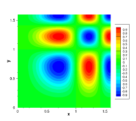
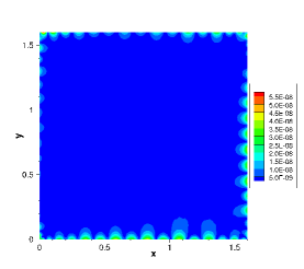
(a) (b) (c)

Figure 3: Variable-coefficient Poisson equation: distributions of (a) the exact solution, (b) the absolute error of the HLConcELM solution, and (c) the absolute error of the conventional ELM solution. In (b,c), network architecture $\mathbf{M}=[2,800,50,1]$, Gaussian activation function, $Q=35\times 35$ uniform collocation points. $\mathbf{R}=(3.0,0.005)$ for HLConcELM in (b). $R_{m}=R_{m0}=0.35$ for conventional ELM in (c), where $R_{m0}$ is the optimal $R_{m}$ computed using the method of DongY2021 .

The first numerical test involves the 2D Poisson equation with a variable coefficient field. Consider the 2D domain $\Omega=[0,1.6]\times[0,1.6]$ and the the following boundary value problem on $\Omega$,

$$\frac{\partial}{\partial x}\left(a(x,y)\frac{\partial u}{\partial x}\right)+\frac{\partial}{\partial y}\left(a(x,y)\frac{\partial u}{\partial y}\right)=f(x,y),$$ (21a)

$$u(0,y)=g_{1}(y),\quad u(1.6,y)=g_{2}(y),\quad u(x,0)=h_{1}(x),\quad u(x,1.6)=h_{2}(x),$$ (21b)

where $(x,y)$ are the spatial coordinates, $u(x,y)$ is the field function to be solved for, $f(x,y)$ is a prescribed source term, $a(x,y)$ is the coefficient field given by $a(x,y)=2+\sin(x+y)$, and $g_{1}$, $g_{2}$, $h_{1}$ and $h_{2}$ are prescribed boundary distributions. We choose the source term $f$ and the boundary data $g_{i}$ and $h_{i}$ ($i=1,2$) appropriately such that the following function satisfies the system (21),

$$u(x,y)=-\sin(\pi x^{2})\sin(\pi y^{2}).$$ (22)

The distribution of this exact solution in the $xy$ plane is illustrated by Figure 3(a).

We employ the HLConcELM method from Section 2 to solve the system (21). Let the vector $\mathbf{M}=[2,m_{1},\dots,m_{L-1},1]$ denote the architecture of the HLConcELM, where the two input nodes represent the coordinates $x$ and $y$ and the single output node represents the solution $u$. We employ the Gaussian activation function for all the hidden nodes, as stated at the beginning of Section 3. The output layer is linear and has no bias. The number of hidden layers and the number of hidden nodes are varied, and the specific architure will be given below when discussing the results.

We employ a uniform set of $Q=Q_{1}\times Q_{1}$ grid points on the domain $\Omega$, with $Q_{1}$ uniform points on each side of the boundary, as the collocation points for training the neural network. $Q_{1}$ is varied in the tests. As discussed earlier, after the neural network is trained, we evaluate the neural network on another finer set of $Q_{eval}=Q_{2}\times Q_{2}$, with $Q_{2}=101$, uniform grid points on $\Omega$ and compute the HLConcELM errors.

Figures 3(b) and (c) show a comparison of the absolute-error distributions in the $xy$ plane of the HLConcELM solution and the conventional ELM solution obtained using a neural network with a narrow last hidden layer. Note that in conventional ELM the usual feedforward neural network has been employed (see Figure 1(a)). For both HLConcELM and conventional ELM we employ here a neural network with the architecture $\mathbf{M}=[2,800,50,1]$ and a uniform set of $Q=35\times 35$ collocation points for the network training. With HLConcELM, for setting the random hidden-layer coefficients, we employ a hidden magnitude vector $\mathbf{R}=(3.0,0.005)$, which is close to the optimum $\mathbf{R}^{*}$ obtained based on the method of DongY2021 . With conventional ELM, we set the hidden-layer coefficients to uniform random values generated on the interval $[-R_{m},R_{m}]$ with $R_{m}=R_{m0}$, where $R_{m0}=0.35$ is the optimal $R_{m}$ obtained using the method of DongY2021 for this case. Because the last hidden layer is quite narrow (with $50$ nodes), we observe that the result of the conventional ELM exhibits no accuracy, with a maximum error around $85$ in the domain. In contrast, the HLConcELM method produces highly accurate results, with the maximum error on the order of $10^{-8}$ in the domain.

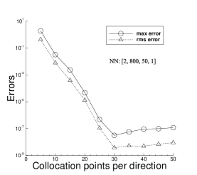
(a) (b)

Figure 4: Variable-coefficient Poisson equation: the maximum/rms errors of the HLConcELM solution versus the number of collocation points per direction obtained with a network architecture of (a) $[2,800,50,1]$ and (b) $[2,50,800,1]$. $\mathbf{R}=(3.0,0.005)$ in (a), and $\mathbf{R}=(0.68,0.82)$ in (b).

Figure 4 illustrates the convergence behavior of the HLConcELM solution with respect to the number of collocation points in the network training. Two neural networks are considered, with the architectures given by $\mathbf{M}_{1}=[2,800,50,1]$ and $\mathbf{M}_{2}=[2,50,800,1]$, respectively. We vary the number of collocation points per direction (i.e. $Q_{1}$) systematically between $Q_{1}=5$ and $Q_{1}=50$, and record the corresponding HLConcELM errors. Figures 4(a) and (b) show the maximum/rms errors of HLConcELM as a function of $Q_{1}$ for the two neural networks. For the network $\mathbf{M}_{1}$ we employ a hidden magnitude vector $\mathbf{R}=(3.0,0.005)$, and for the network $\mathbf{M}_{2}$ we employ a hidden magnitude vector $\mathbf{R}=(0.68,0.82)$. These $\mathbf{R}$ values are obtained using the method of DongY2021 . The results indicate that the HLConcELM errors decrease approximately exponentially with increasing number of collocation points (when $Q_{1}\leqslant 30$). The errors stagnate as $Q_{1}$ increases further, because of the fixed network size. Note that the last hidden layer of the network $\mathbf{M}_{1}$ is quite narrow ($50$ nodes), while that of the network $\mathbf{M}_{2}$ is quite wide ($800$ nodes). The HLConcELM method produces accurate results with both types of neural networks.

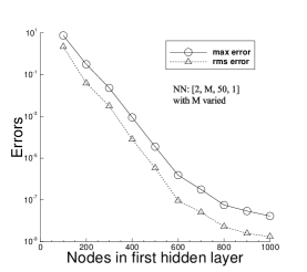
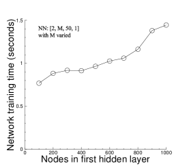
(a) (b)

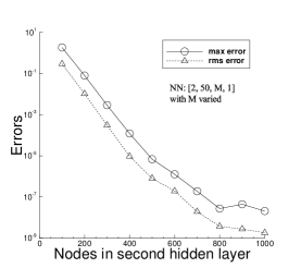
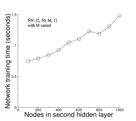
(c) (d)

Figure 5: Variable-coefficient Poisson equation: (a) The maximum/rms errors and (b) the network training time of HLConcELM versus the number of nodes in the first hidden layer for a network architecture $[2,M,50,1]$ (varying $M$). (c) The maximum/rms errors and (d) the network training time of HLConcELM versus the number of nodes in the second hidden layer for a network architecture $[2,50,M,1]$ (varying $M$). $Q=35\times 35$ uniform collocation points in (a,b,c,d). $\mathbf{R}=(3.0,0.005)$ in (a,b), and $\mathbf{R}=(0.68,0.82)$ in (c,d).

Figure 5 illustrates the convergence behavior, as well as the network training time, of the HLConcELM method with respect to the number of nodes in the neural network. We consider two groups of neural networks, with the architectures given by $\mathbf{M}_{1}=[2,M,50,1]$ and $\mathbf{M}_{2}=[2,50,M,1]$, respectively, where $M$ is varied systematically between $M=100$ and $M=1000$. For all the test cases, we employ a fixed uniform set of $Q=35\times 35$ collocation points to train the neural network. For generating the hidden-layer coefficients, we use a hidden magnitude vector $\mathbf{R}=(3.0,0.005)$ with the first group of networks $\mathbf{M}_{1}$, and a vector $\mathbf{R}=(0.68,0.82)$ with the second group of networks $\mathbf{M}_{2}$. Figures 5(a) and (c) depict the maximum/rms errors of HLConcELM as a function of $M$ for these two groups of neural networks. Figures 5(b) and (d) depict the corresponding wall time it takes to train these neural networks with HLConcELM. It can be observed that the HLConcELM errors decrease approximately exponentially with increasing $M$ (before saturation). When $M$ becomes large the HLConcELM results are highly accurate. The network training time of the HLConcELM method increases approximately linearly with increasing $M$. In the range of $M$ values tested here, it takes around a second to train the neural network to attain the HLConcELM results.

network	collocation	current	HLConcELM	conventional	ELM
architecture	points	max error	rms error	max error	rms error
$[2,800,50,1]$	$5\times 5$	$1.91E+0$	$4.31E-1$	$3.06E+1$	$6.34E+0$
	$10\times 10$	$3.22E-2$	$7.88E-3$	$5.48E+1$	$1.78E+1$
	$15\times 15$	$2.33E-3$	$3.92E-4$	$6.24E+1$	$2.11E+1$
	$20\times 20$	$4.70E-5$	$1.32E-5$	$6.97E+1$	$2.42E+1$
	$25\times 25$	$4.78E-7$	$1.10E-7$	$7.67E+1$	$2.70E+1$
	$30\times 30$	$3.17E-8$	$3.79E-9$	$8.31E+1$	$2.96E+1$
$[2,50,800,1]$	$5\times 5$	$2.95E+0$	$9.26E-1$	$2.48E+0$	$8.85E-1$
	$10\times 10$	$9.35E-2$	$9.93E-3$	$1.32E-1$	$1.50E-2$
	$15\times 15$	$1.11E-3$	$2.40E-4$	$6.52E-3$	$1.00E-3$
	$20\times 20$	$3.42E-5$	$6.91E-6$	$7.63E-5$	$1.33E-5$
	$25\times 25$	$2.34E-6$	$4.45E-7$	$1.83E-6$	$4.14E-7$
	$30\times 30$	$3.07E-8$	$4.81E-9$	$9.87E-8$	$2.02E-8$

Table 1: Variable-coefficient Poisson equation: Comparison of the maximum/rms errors computed using the current HLConcELM method and the conventional ELM method. The HLConcELM data in this table correspond to a portion of those in Figure 4(a) for the network $[2,800,50,1]$ and to those in Figure 4(b) for the network $[2,50,800,1]$. For conventional ELM, the random hidden-layer coefficients are assigned to uniform random values generated on $[-R_{m},R_{m}]$ with $R_{m}=R_{m0}$. Here $R_{m0}$ is the optimal $R_{m}$ obtained using the method of DongY2021 , with $R_{m0}=0.35$ for the network $[2,800,50,1]$ and $R_{m0}=0.75$ for the network $[2,50,800,1]$.

Table 1 provides a comparison of the HLConcELM accuracy and the conventional ELM accuracy for solving the variable-coefficient Poisson equation on two network architectures, $\mathbf{M}_{1}=[2,800,50,1]$ and $\mathbf{M}_{2}=[2,50,800,1]$. The network $\mathbf{M}_{1}$ contains a relatively small number of nodes in its last hidden layer, and the conventional ELM would not perform well. The network $\mathbf{M}_{2}$ contains a large number of nodes in its last hidden layer, and the conventional ELM should perform quite well. We consider a sequence of uniform collocation points, ranging from $Q=5\times 5$ to $Q=30\times 30$. Table 1 lists the maximum/rms errors of the HLConcELM solution and the conventional ELM solution corresponding to each set of collocation points. The data indicate that the conventional ELM exhibits no accuracy with the network $\mathbf{M}_{1}$, and exhibits exponentially increasing accuracy with increasing collocation points on the network $\mathbf{M}_{2}$. On the other hand, the current HLConcELM method exhibits exponentially increasing accuracy with increasing collocation points on both networks $\mathbf{M}_{1}$ and $\mathbf{M}_{2}$.

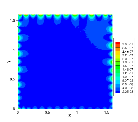
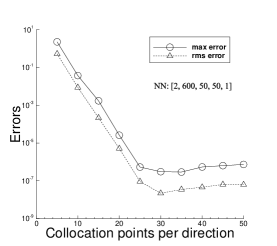
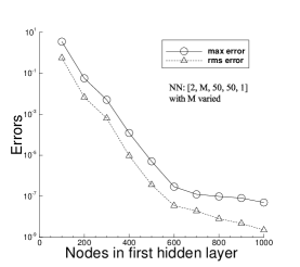
(a) (b) (c)

Figure 6: Variable-coefficient Poisson equation (3 hidden layers in NN): (a) Distribution of the absolute error of the HLConcELM solution. The maximum/rms errors of HLConcELM versus (b) the number of collocation points per direction, and (c) the number of the nodes in the first hidden layer of the neural network. Neural network architecture $\mathbf{M}=[2,M,50,50,1]$, $Q=Q_{1}\times Q_{1}$ uniform collocation points. $M=600$ in (a,b) and is varied in (c). $Q_{1}=35$ in (a,c) and is varied in (b). $\mathbf{R}=(2.6,0.005,0.8)$ in (a,b,c).

Figure 6 is an illustration of the HLConcELM results obtained on neural networks with three hidden layers. Here we consider a network architecture $\mathbf{M}=[2,M,50,50,1]$, with $M$ either fixed at $M=600$ or varied systematically between $M=100$ and $M=1000$. The set of collocation points (uniform) is either fixed at $Q=35\times 35$ or varied systematically between $Q=5\times 5$ and $Q=50\times 50$. We employ a fixed hidden magnitude vector $\mathbf{R}=(2.6,0.005,0.8)$, obtained using the method of DongY2021 . Figure 6(a) shows the HLConcELM error distribution corresponding to $\mathbf{M}=[2,600,50,50,1]$ and $Q=35\times 35$, indicating a quite high accuracy, with the maximum error in the domain on the order $10^{-7}$. Figures 6(b) and (c) demonstrate the exponential convergence (before saturation) of the HLConcELM errors with respect to the collocation points $Q_{1}$ and the number of nodes $M$, respectively. These results show that the current HLConcELM method can produce highly accurate results on neural networks with multiple hidden layers and a narrow last hidden layer.

3.2 Advection Equation

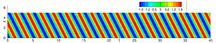
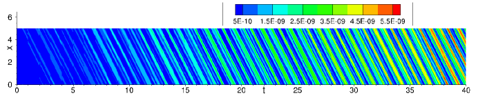
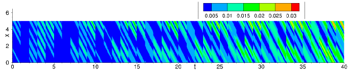
(a) (b) (c)

Figure 7: Advection equation: Distributions in the spatial-temporal domain of (a) the exact solution, (b) the absolute error of the HLConcELM solution, and (c) the absolute error of the conventional ELM solution. In (b,c), network architecture [2, 500, 50, 1], $40$ uniform time blocks, $Q=35\times 35$ uniform collocation points per time block. $\mathbf{R}=(3.0,1.0)$ in (b) for HLConcELM. $R_{m}=R_{m0}=0.065$ in (c) for conventional ELM.

In the next example we employ the 1D advection equation (plus time) to test the HLConcELM method. Consider the spatial-temporal domain, $(x,t)\in\Omega=[0,5]\times[0,40]$, and the following initial/boundary value problem on $\Omega$,

$$\frac{\partial u}{\partial t}-2\frac{\partial u}{\partial x}=0,$$ (23a)

$$u(0,t)=u(5,t),$$ (23b)

$$u(x,0)=20\tanh\left(\frac{1}{10}\cos\left(\frac{2\pi}{5}\left(x-3\right)\right)\right).$$ (23c)

In the above equations $u(x,t)$ is the field function to be solved for, and we impose the periodic boundary condition in the spatial direction. This system has the following exact solution,

$$u(x,t)=20\tanh\left(\frac{1}{10}\cos\left(\frac{2\pi}{5}\left(x+2t-3\right)\right)\right).$$ (24)

The distribution of this solution on the spatial-temporal domain is illustrated in Figure 7(a).

To solve the system (23), we employ the HLConcELM method combined with the block time marching scheme (see Remark 2.5 and DongL2021 ). We divide the domain $\Omega$ into $40$ uniform time blocks in time. For computing each time block with HLConcELM, we employ a network architecture $\mathbf{M}=[2,m_{1},\dots,m_{L-1},1]$, where the two input nodes represent $x$ and $t$ and the single output node represents $u(x,t)$. Let $Q=Q_{1}\times Q_{1}$ denote the uniform set of collocation points for each time block ($Q_{1}$ grid points in both $x$ and $t$ directions), where $Q_{1}$ is varied in the tests. As discussed before, upon completion of training, the neural network is evaluated on a uniform set of $Q_{eval}=101\times 101$ grid points on each time block and the corresponding errors are computed. The maximum and rms errors reported below refer to the errors of the HLConcELM solution on the entire domain $\Omega$ (over $40$ time blocks).

Figures 7(b) and (c) illustrate the absolute-error distributions on $\Omega$ of the HLConcELM solution and the conventional ELM solution, respectively. For both methods, we employ $40$ time blocks in block time marching, a neural network architecture $\mathbf{M}=[2,500,50,1]$ with the Gaussian activation function, and a set of $Q=35\times 35$ uniform collocation points per time block. For HLConcELM we employ $\mathbf{R}=(3.0,1.0)$, which is computed by the method of DongY2021 . For conventional ELM we employ $R_{m}=R_{m0}=0.065$, which is also obtained by the method of DongY2021 , for generating the random hidden-layer coefficients. Because the number of nodes in the last hidden layer is quite small, the conventional ELM exhibits a low accuracy, with the maximum error on the order of $10^{-2}$ in the domain. On the other hand, the HLConcELM method produces a highly accurate solution, with the maximum error on the order of $10^{-9}$ in the domain.

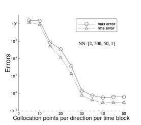
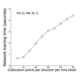
(a) (b)

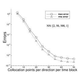
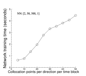
(c) (d)

Figure 8: Advection equation: The maximum/rms errors in the domain $\Omega$ (a,c) and the network training time (b,d) of HLConcELM versus the number of collocation points per direction in each time block. The results are attained with two network architectures: (a,b) $\mathbf{M}_{1}=[2,500,50,1]$, and (c,d) $\mathbf{M}_{2}=[2,50,500,1]$. $\mathbf{R}=(3.0,1.0)$ in (a,b) for the network $\mathbf{M}_{1}$, and $\mathbf{R}=(0.9,0.5)$ in (c,d) for the network $\mathbf{M}_{2}$.

Figure 8 illustrates the convergence behavior, as well as the growth in the network training time, of the HLConcELm method with respect to the number of collocation points. We have considered two network architectures, $\mathbf{M}_{1}=[2,500,50,1]$ and $\mathbf{M}_{2}=[2,50,500,1]$, with a narrower last hidden layer in $\mathbf{M}_{1}$ and a wider one in $\mathbf{M}_{2}$. A uniform set of $Q=Q_{1}\times Q_{1}$ collocation points is employed, with $Q_{1}$ varied systematically between $Q_{1}=5$ and $Q_{1}=50$ in the tests. The hidden magnitude vector $\mathbf{R}$ computed by the method DongY2021 is used in the simulations, with $\mathbf{R}=(3.0,1.0)$ for the network $\mathbf{M}_{1}$ and $\mathbf{R}=(0.9,0.5)$ for the network $\mathbf{M}_{2}$. Figures 8(a) and (b) depict the maximum/rms errors on $\Omega$ and the network training time, respectively, as a function of $Q_{1}$ obtained with the neural network $\mathbf{M}_{1}$. Figures 8(c) and (d) show the corresponding results obtained with the network $\mathbf{M}_{2}$. While the convergence behavior is not quite regular, one can observe that the HLConcELM errors approximately decrease exponentially (before saturation) with increasing number of collocation points. The network training time grows approximately linearly with increasing number of training collocation points.

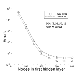
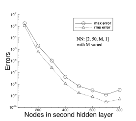
(a) (b)

Figure 9: Advection equation: (a) The HLConcELM maximum/rms errors on $\Omega$ versus the number of nodes in the first hidden layer for the network architecture $\mathbf{M}_{1}=[2,M,50,1]$ (varying $M$). (b) The HLConcELM maximum/rms errors on $\Omega$ versus the number of nodes in the second hidden layer for the network architecture $\mathbf{M}_{2}=[2,50,M,1]$ (varying $M$). $Q=35\times 35$ in (a,b). $\mathbf{R}=(3.0,1.0)$ in (a) for the network $\mathbf{M}_{1}$, and $\mathbf{R}=(0.9,0.5)$ in (b) for the network $\mathbf{M}_{2}$.

Figure 9 illustrates the convergence behavior of the HLConcELM method with respect to the number of nodes in the neural network. Two groups of neural networks are considered in these tests, with an architecture $\mathbf{M}_{1}=[2,M,50,1]$ for the first group and $\mathbf{M}_{2}=[2,50,M,1]$ for the second one, with $M$ varied systematically. A uniform set of $Q=35\times 35$ collocation points is employed for training the neural networks. We use $\mathbf{R}=(3.0,1.0)$ for the architecture $\mathbf{M}_{1}$ and $\mathbf{R}=(0.9,0.5)$ for the architecture $\mathbf{M}_{2}$. The plots (a) and (b) show the maximum/rms errors of HLConcELM on $\Omega$ as a function of $M$, indicating that the errors decrease approximately exponentially (before saturation) with increasing $M$ in the neural network.

network	collocation	current	HLConcELM	conventional	ELM
architecture	points	max error	rms error	max error	rms error
$[2,500,50,1]$	$5\times 5$	$2.48E+0$	$1.41E+0$	$1.33E+0$	$4.57E-1$
	$10\times 10$	$2.21E+0$	$8.26E-1$	$5.97E-2$	$1.91E-2$
	$15\times 15$	$7.45E-3$	$2.78E-3$	$4.31E-2$	$1.30E-2$
	$20\times 20$	$1.22E-3$	$1.39E-4$	$3.62E-2$	$1.08E-2$
	$25\times 25$	$1.39E-5$	$2.00E-6$	$3.15E-2$	$9.50E-3$
	$30\times 30$	$2.25E-8$	$6.47E-9$	$3.24E-2$	$8.89E-3$
$[2,50,500,1]$	$5\times 5$	$1.97E+0$	$1.10E+0$	$1.86E+0$	$9.18E-1$
	$10\times 10$	$9.33E-2$	$3.74E-2$	$4.18E-2$	$1.65E-2$
	$15\times 15$	$1.05E-3$	$4.16E-4$	$3.09E-4$	$8.48E-5$
	$20\times 20$	$3.16E-5$	$6.30E-6$	$1.97E-4$	$5.01E-5$
	$25\times 25$	$5.60E-7$	$1.36E-7$	$7.60E-5$	$5.85E-6$
	$30\times 30$	$5.80E-8$	$1.45E-8$	$9.76E-8$	$3.32E-8$

Table 2: Advection equation: Comparison of the maximum/rms errors on $\Omega$ from the current HLConcELM method and the conventional ELM method DongL2021 . The HLConcELM data in this table correspond to a portion of those in Figure 8(a) for the network $[2,500,50,1]$ and to those in Figure 8(c) for the network $[2,50,500,1]$. For conventional ELM, the hidden-layer coefficients are set to uniform random values generated on $[-R_{m},R_{m}]$ with $R_{m}=R_{m0}$. Here $R_{m0}$ is the optimal $R_{m}$ computed by the method of DongY2021 , with $R_{m0}=0.065$ for the network $[2,500,50,1]$ and $R_{m0}=0.65$ for the network $[2,50,500,1]$.

Table 2 provides an accuracy comparison of the current HLConcELM method and the conventional ELM method DongL2021 for solving the advection equation. Two neural networks are considered here, with the architectures given by $\mathbf{M}_{1}=[2,500,50,1]$ and $\mathbf{M}_{2}=[2,50,500,1]$, respectively. The maximum/rms errors of both methods on the domain $\Omega$ corresponding to a sequence of collocation points are listed in the table. With the network $\mathbf{M}_{1}$, whose last hidden layer is narrower, the conventional ELM exhibits only a fair accuracy with increasing collocation points, with its maximum errors on the order of $10^{-2}$. In contrast, the current HLConcELM method produces highly accurate results with the network $\mathbf{M}_{1}$, with the maximum error reaching the order of $10^{-8}$ on the larger set of collocation points. With the network $\mathbf{M}_{2}$, whose last hidden layer is wider, both the conventional ELM and the current HLConcELM produce highly accurate results with increasing number of collocation points. These observations are consistent with those in the previous subsection for the variable-coefficient Poisson equation.

(a)

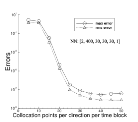
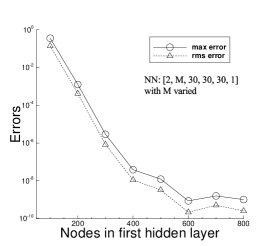
(b) (c)

Figure 10: Advection equation (4 hidden layers in neural network): (a) Error distribution of the HLConcELM solution on $\Omega$. The HLConcELM maximum/rms errors on $\Omega$ versus (b) the number of collocation points per direction in each time block, and (c) the number of nodes in the first hidden layer ($M$). Network architecture $[2,M,30,30,30,1]$, $40$ time blocks in block time marching. $Q=35\times 35$ in (a,c), and is varied in (b). $M=400$ in (a,b), and is varied in (c). $\mathbf{R}=(3.1,1.0,0.9,0.8)$ in (a,b,c).

Figure 10 illustrates the HLConcELM results obtained on a deeper neural network containing $4$ hidden layers for solving the advection equation. The network architecture is given by $\mathbf{M}=[2,M,30,30,30,1]$, where $M$ is either fixed at $M=400$ or varied systematically between $M=100$ and $M=800$. A uniform set of $Q=Q_{1}\times Q_{1}$ collocation points is used to train the network, where $Q_{1}$ is either fixed at $Q_{1}=35$ or varied systematically between $Q_{1}=5$ and $Q_{1}=50$. In all simulations we employ a hidden magnitude vector $\mathbf{R}=(3.1,1.0,0.9,0.8)$, which is computed using the method of DongY2021 . Figure 10(a) depicts the distribution of the absolute error of the HLConcELM solution on $\Omega$, which corresponds to $M=400$ and $Q_{1}=35$. It can be observed that the result is highly accurate, with a maximum error on the order of $10^{-8}$ in the domain. Figure 10(b) shows the maximum/rms errors of HLConcELM as a function of $Q_{1}$, with a fixed $M=400$ in the tests. Figure 10(c) shows the maximum/rms errors of HLConcELM as a function of $M$ in the neural network, with a fixed $Q_{1}=35$ for the collocation points. The exponential convergence of the HLConcELM errors (before saturation) is unmistakable.

3.3 Nonlinear Helmholtz Equation

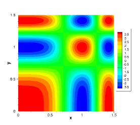
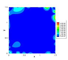
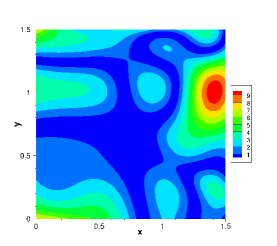
(a) (b) (c)

Figure 11: Nonlinear Helmholtz equation: Distributions of (a) the exact solution, (b) the absolute error of the HLConcELM solution, and (c) the absolute error of the conventional ELM solution. In (b,c), network architecture $[2,500,30,1]$, Gaussian activation function, $Q=35\times 35$ uniform collocation points. $\mathbf{R}=(2.0,3.0)$ in (b) for HLConcELM. $R_{m}=R_{m0}=0.6$ in (c) for conventional ELM.

We employ a nonlinear Helmholtz equation to test the HLConcELM method for the next problem. Consider the 2D domain $(x,y)\in\Omega=[0,1.5]\times[0,1.5]$ and the following boundary value problem on $\Omega$,

$$\frac{\partial^{2}u}{\partial x^{2}}+\frac{\partial^{2}u}{\partial y^{2}}-100u+10\cosh(u)=f(x,y),$$ (25a)

$$u(0,y)=g_{1}(y),\quad u(1.5,y)=g_{2}(y),\quad u(x,0)=h_{1}(x),\quad u(x,1.5)=h_{2}(x).$$ (25b)

In the above equations $u(x,y)$ is the field solution to be sought, $f(x,y)$ is a prescribed source term, $g_{i}$ and $h_{i}$ ($i=1,2$) are the Dirichlet boundary data. In this subsection we choose $f$, $g_{i}$ and $h_{i}$ ($i=1,2$) such that the system (25) has the following solution,

$$u(x,y)=4\cos\left(\pi x^{2}\right)\cos\left(\pi y^{2}\right).$$ (26)

The distribution of this solution in the $xy$ plane is illustrated in Figure 11(a).

We employ the HLConcELM method with neural networks that contain two input nodes, representing the $x$ and $y$, and a single output node, representing the solution $u$. The number of hidden layers and the number of hidden nodes are varied and will be specified below. To train the neural network, we employ a uniform set of $Q=Q_{1}\times Q_{1}$ collocation points on $\Omega$, with $Q_{1}$ varied in the tests. The ELM errors reported below are computed on a finer set of $Q_{eval}=101\times 101$ uniform grid points, as explained before.

Figures 11(b) and (c) illustrate the absolute-error distributions obtained using the HLConcELM method and the conventional ELM method with the network architecture $\mathbf{M}=[2,500,30,1]$. A uniform set of $Q=35\times 35$ collocation points has been used to train the network with both methods. The hidden magnitude vector is $\mathbf{R}=(2.0,3.0)$ for HLConcELM, which is obtained with the method of DongY2021 . For conventional ELM we have employed $R_{m}=R_{m0}=0.6$, which is also obtained using the method of DongY2021 , for generating the random hidden-layer coefficients. The conventional ELM solution is inaccurate, with the maximum error on order of $10$. On the other hand, the current HLConcELM method produces an accurate solution on the same network architecture, with the maximum error on the order of $10^{-6}$ in the domain.

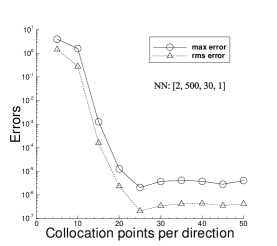
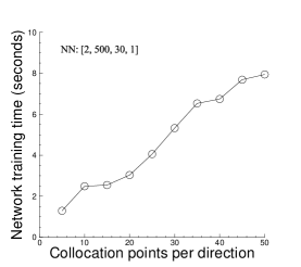
(a) (b)

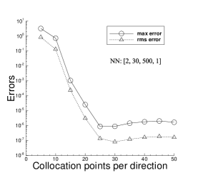
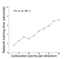
(c) (d)

Figure 12: Nonlinear Helmholtz equation: The maximum/rms errors (a,c) and the network training time (b,d) of the HLConcELM method versus the number of collocation points in each direction. In (a,b), network architecture $[2,500,30,1]$, $\mathbf{R}=(2.0,3.0)$. In (c,d), network architecture $[2,30,500,1]$, $\mathbf{R}=(0.65,0.7)$. In (a,b,c,d), uniform collocation points $Q=Q_{1}\times Q_{1}$, with $Q_{1}$ varied.

Figure 12 illustrates the convergence behavior and the network training time with respect to the training collocation points of the HLConcELM method for solving the nonlinear Helmholtz equation. Two network architectures are considered here, $\mathbf{M}_{1}=[2,500,30,1]$ and $\mathbf{M}_{2}=[2,30,500,1]$. The number of collocation points in each direction ($Q_{1}$) is varied systematically between $Q_{1}=5$ and $Q_{1}=50$ in these tests. We employ $\mathbf{R}=(2.0,3.0)$ for the network $\mathbf{M}_{1}$ and $\mathbf{R}=(0.65,0.7)$ for the network $\mathbf{M}_{2}$, which are obtained using the method of DongY2021 . Figures 12(a) and (b) show the maximum/rms errors and the network training time of the HLConcELM method as a function of $Q_{1}$ for the neural network $\mathbf{M}_{1}$. Figures 12(c) and (d) show the corresponding results for the network $\mathbf{M}_{2}$. The exponential convergence (before saturation) and the near linear growth in the network training time observed here for the nonlinear Helmholtz equation are consistent with those for the linear problems in previous subsections.

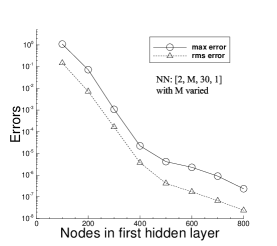
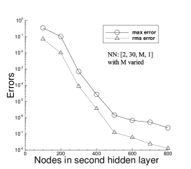
(a) (b)

Figure 13: Nonlinear Helmholtz equation: (a) The HLConcELM maximum/rms errors versus the number of nodes in the first hidden layer with network architecture $[2,M,30,1]$ ($M$ varied). (b) The HLConcELM maximum/rms errors versus the number of nodes in the second hidden layer with the architecture $[2,30,M,1]$ ($M$ varied). $Q=35\times 35$ collocation points in (a,b). $\mathbf{R}=(2.0,3.0)$ in (a), and $\mathbf{R}=(0.65,0.7)$ in (b).

Figure 13 illustrates the error convergence of the HLConcELM method with respect to the number of nodes in the neural network. Two groups of neural networks are considered here, with the architectures $\mathbf{M}_{1}=[2,M,30,1]$ and $\mathbf{M}_{2}=[2,30,M,1]$, where $M$ is varied systematically. The networks are trained on a uniform set of $Q=35\times 35$ collocation points. The plots (a) and (b) show the maximum/rms errors of HLConcELM as a function of $M$ for these two groups of neural networks. It can be observed that the errors decrease approximately exponentially with increasing $M$.

network	collocation	current	HLConcELM	conventional	ELM
architecture	points	max error	rms error	max error	rms error
$[2,500,30,1]$	$5\times 5$	$4.00E+0$	$1.48E+0$	$7.64E+0$	$2.41E+0$
	$10\times 10$	$1.59E+0$	$2.80E-1$	$9.69E+0$	$2.73E+0$
	$15\times 15$	$1.27E-3$	$1.62E-4$	$9.73E+0$	$2.71E+0$
	$20\times 20$	$1.27E-5$	$2.34E-6$	$9.74E+0$	$2.73E+0$
	$25\times 25$	$2.08E-6$	$2.11E-7$	$9.74E+0$	$2.73E+0$
	$30\times 30$	$3.74E-6$	$3.48E-7$	$9.75E+0$	$2.74E+0$
$[2,30,500,1]$	$5\times 5$	$3.23E+0$	$8.43E-1$	$3.80E+0$	$1.15E+0$
	$10\times 10$	$7.22E-1$	$1.32E-1$	$3.08E+0$	$7.48E-1$
	$15\times 15$	$1.06E-3$	$2.36E-4$	$3.86E-4$	$6.29E-5$
	$20\times 20$	$2.56E-5$	$3.12E-6$	$3.15E-5$	$5.67E-6$
	$25\times 25$	$8.78E-7$	$1.38E-7$	$1.33E-6$	$2.68E-7$
	$30\times 30$	$8.99E-7$	$8.20E-8$	$1.76E-6$	$1.92E-7$

Table 3: Nonlinear Helmholtz equation: Comparison of the maximum/rms errors from the HLConcELM method and the conventional ELM method DongL2021 . The HLConcELM data in this table correspond to a portion of those in Figure 12(a) for the network $[2,500,30,1]$ and to those in Figure 12(c) for the network $[2,30,500,1]$. For conventional ELM, the hidden-layer coefficients are set to uniform random values generated on $[-R_{m},R_{m}]$ with $R_{m}=R_{m0}$. Here $R_{m0}$ is the optimal $R_{m}$ obtained using the method of DongY2021 , with $R_{m0}=0.6$ for the network $[2,500,30,1]$ and $R_{m0}=0.65$ for the network $[2,30,500,1]$.

Table 3 compares the numerical errors of the current HLConcELM method and the conventional ELM method for solving the nonlinear Helmholtz equation on two network architectures, $\mathbf{M}_{1}=[2,500,30,1]$ and $\mathbf{M}_{2}=[2,30,500,1]$, trained on a sequence of uniform sets of collocation points. The HLConcELM method produces highly accurate results on both neural networks. On the other hand, while the conventional ELM produces accurate results on the network $\mathbf{M}_{2}$, its solution on the network $\mathbf{M}_{1}$ is utterly inaccurate.

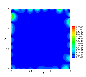
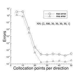
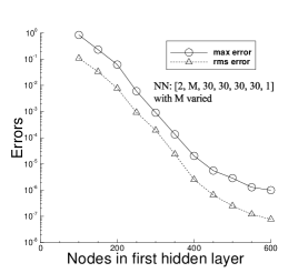
(a) (b) (c)

Figure 14: Nonlinear Helmholtz equation (5 hidden layers in neural network): (a) Error distribution of the HLConcELM solution. The maximum/rms errors of the HLConcELM solution versus (b) the number of collocation points in each direction and (c) the number of nodes in the first hidden layer ($M$). Neural network architecture $[2,M,30,30,30,30,1]$, $Q=Q_{1}\times Q_{1}$ uniform collocation points. $M=500$ in (a,b), and is varied in (c). $Q_{1}=35$ in (a,c), and is varied in (b). $\mathbf{R}=(2.1,0.1,2.0,2.5,0.5)$ in (a,b,c).

Figure 14 illustrates the HLConcELM results computed on a deeper neural network with $5$ hidden layers. The network architecture is given by $\mathbf{M}=[2,M,30,30,30,30,1]$, where $M$ is either fixed at $M=500$ or varied systematically in the tests. The network is trained on a uniform set of $Q=Q_{1}\times Q_{1}$ collocation points, where $Q_{1}$ is either fixed at $Q_{1}=35$ or varied systematically. Figure 14(a) depicts the absolute-error distribution of the HLConcELM solution obtained with $M=500$ and $Q_{1}=35$, indicating a quite high accuracy with the maximum error on the order of $10^{-6}$ in the domain. Figures 14(b) and (c) shows the HLConcELM errors as a function of $Q_{1}$ and $M$, respectively. The exponential convergence (prior to saturation) of these errors is evident.

3.4 Burgers’ Equation

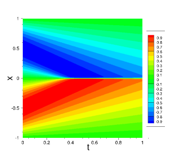
Figure 15: Burgers’ equation: distribution of the exact solution.

In the next benchmark example we use the viscous Burgers’ equation to test the performance of the HLConcELM method. Consider the spatial-temporal domain, $(x,t)\in\Omega=[-1,1]\times[0,1]$, and the following initial/boundary value problem on $\Omega$,

$$\frac{\partial u}{\partial t}+u\frac{\partial u}{\partial x}=\nu\frac{\partial^{2}u}{\partial x^{2}},$$ (27a)

$$u(-1,t)=u(1,t)=0,$$ (27b)

$$u(x,0)=-\sin(\pi x),$$ (27c)

where $\nu=\frac{1}{100\pi}$, and $u(x,t)$ denotes the field function to be solved for. This problem has the following exact solution Basdevant1986 ,

$$u(x,t)=-\frac{\int_{-\infty}^{\infty}\sin\pi(x-\eta)f(x-\eta)e^{-\frac{\eta^{2}}{4\nu t}}d\eta}{\int_{-\infty}^{\infty}f(x-\eta)e^{-\frac{\eta^{2}}{4\nu t}}d\eta},$$ (28)

where $f(y)=e^{-\frac{\cos(\pi y)}{2\pi\nu}}$. Figure 15 illustrates the distribution of this solution on the spatial-temporal domain, which indicates that a sharp gradient develops in the domain over time.

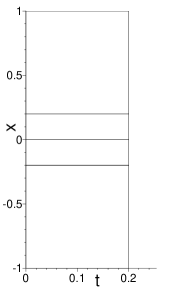
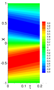
(a) (b) (c)

Figure 16: Burgers’s equation on the smaller domain $\Omega_{1}$ ($t\in[0,0.2]$): (a) Configuration of the $4$ sub-domains in the locHLConcELM simulation. Distributions of the locHLConcELM solution (b) and its absolute error (c) on $\Omega_{1}$. Local neural-network architecture: [2, 200, 30, 1], $Q=21\times 21$ uniform collocation points per sub-domain, $\mathbf{R}=(0.9,0.05)$.

We will first solve the problem (27) on a smaller domain (with a smaller temporal dimension) $\Omega_{1}=[-1,1]\times[0,0.2]$, before the sharp gradient develops, in order to investigate the convergence behavior of the HLConcELM method. Then we will compute this problem on the larger domain $\Omega$ using HLConcELM.

On the smaller domain $\Omega_{1}$ we solve the system (27) by the locHLConcELM method (local version of HLConcELM, see Remark 2.6). We partition $\Omega_{1}$ along the $x$ direction into $4$ sub-domains; see Figure 16(a). These sub-domains are non-uniform, and the $x$ coordinates of the sub-domain boundaries are given by the vector $\bm{\mathcal{X}}=[-1,-0.2,0,0.2,1]$. We impose $C^{1}$ continuity conditions in $x$ across the interior sub-domain boundaries. We employ a HLConcELM for the local neural network on each sub-domain, which contains two input nodes (representing the $x$ and $t$ of the sub-domain) and a single output node (representing the solution $u$ on the sub-domain). The specific architectures of the neural network will be provided below. On each sub-domain we employ a uniform set of $Q=Q_{1}\times Q_{1}$ collocation points ($Q_{1}$ points in both $x$ and $t$ directions) for the network training, with $Q_{1}$ varied in the tests. We train the overall neural network, which consists of the local neural networks coupled together by the $C^{1}$ continuity conditions, by the nonlinear least squares method; see Section 2.3 and also DongL2021 .

Figures 16(b) and (c) illustrate the distributions of the HLConcELM solution and its absolute error on the domain $\Omega_{1}$, respectively. These results are obtained by locHLConcELMs with an architecture $[2,200,30,1]$ and a uniform set of $Q=21\times 21$ collocation points on each sub-domain. The hidden magnitude vector is $\mathbf{R}=(0.9,0.05)$, which is obtained using the method of DongY2021 . The locHLConcELM method produces an accurate solution, with the maximum error on the order of $10^{-7}$ on $\Omega_{1}$.

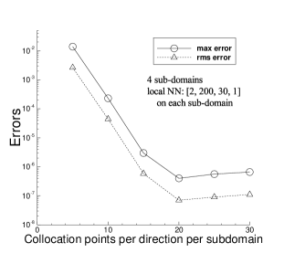
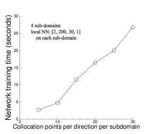
(a) (b)

Figure 17: Burgers’ equation on the smaller domain $\Omega_{1}$: (a) The locHLConcELM maximum/rms errors and (b) the network training time versus the number of collocation points per direction in each sub-domain. Local network architecture: [2, 200, 30, 1], $Q=Q_{1}\times Q_{1}$ uniform collocation points ($Q_{1}$ varied), $\mathbf{R}=(0.9,0.05)$.

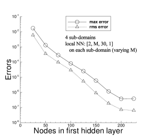
(a) (b)

Figure 18: Burgers’ equation on the smaller domain $\Omega_{1}$: (a) The locHLConcELM maximum/rms errors and (b) the network training time versus the number of nodes in the first hidden layer ($M$). Local network architecture [2, M, 30, 1] ($M$ varied), $Q=21\times 21$ uniform collocation points per sub-domain, $\mathbf{R}=(0.9,0.05)$.

Figure 17 illustrates the convergence behavior and the network training time of the locHLConcELM method with respect to the increase of the collocation points for the smaller domain $\Omega_{1}$. The local network architecture is given by $[2,300,30,1]$, and the collocation points are varied systematically between $Q=5\times 5$ and $Q=30\times 30$ in the tests. The plots (a) and (b) show the locHLConcELM errors and the network training time as a function of the number of collocation points in each direction, respectively. We observe that the locHLConcELM errors decrease exponentially (before saturation) and the network training time grows approximately linearly with increasing collocation points.

Figure 18 is an illustration of the convergence behavior and the network training time of the locHLConcELM method with respect to the size of the neural network. The local network architecture is given by $[2,M,30,1]$, with $M$ varied systematically. We employ a fixed uniform set of $Q=21\times 21$ collocation points, and a hidden magnitude vector $\mathbf{R}=(0.9,0.05)$ obtained using the method of DongY2021 . One observes that the errors decrease exponentially and that the network training time grows superlinearly with increasing $M$.

local network	collocation	current	locHLConcELM	conventional	locELM
architecture	points	max error	rms error	max error	rms error
$[2,200,30,1]$	$5\times 5$	$1.39E-2$	$2.64E-3$	$4.12E-2$	$1.21E-2$
	$10\times 10$	$2.30E-4$	$4.44E-5$	$6.62E-2$	$2.84E-2$
	$15\times 15$	$2.98E-6$	$5.83E-7$	$7.42E-2$	$3.16E-2$
	$20\times 20$	$4.01E-7$	$7.06E-8$	$7.97E-2$	$3.39E-2$
	$25\times 25$	$5.59E-7$	$9.04E-8$	$8.44E-2$	$3.58E-2$
	$30\times 30$	$6.60E-7$	$1.11E-7$	$8.86E-2$	$3.76E-2$

Table 4: Burgers’ equation on the smaller domain $\Omega_{1}$: Comparison of the maximum/rms errors from the locHLConcELM method and the conventional locELM method DongL2021 . The locHLConcELM data in this table correspond to those in Figure 17(a). For conventional locELM, the random hidden-layer coefficients are set to uniform random values generated on $[-R_{m},R_{m}]$ with $R_{m}=R_{m0}=0.175$, where $R_{m0}$ is the optimal $R_{m}$ obtained using the method of DongY2021 .

Table 4 provides an accuracy comparison of the HLConcELM method and the conventional locELM method DongL2021 for solving the Burgers’ equation on the smaller domain $\Omega_{1}$. With both methods, we employ $4$ sub-domains as shown in Figure 16(a), a local neural network architecture $[2,200,30,1]$, and a sequence of uniform collocation points ranging from $Q=5\times 5$ and $Q=30\times 30$. The current locHLConcELM method is significantly more accurate than the conventional locELM method, with their maximum errors on the order of $10^{-7}$ and $10^{-2}$ respectively.

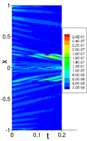
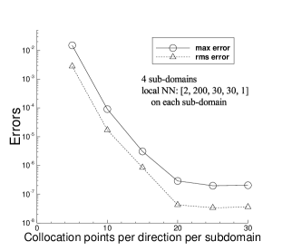
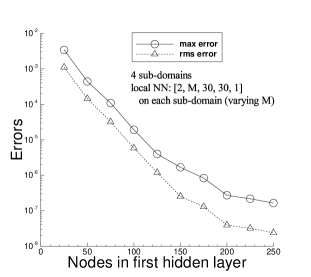
(a) (b) (c)

Figure 19: Burgers’ equation on the smaller domain $\Omega_{1}$ ($3$ hidden layers in network): (a) Error distribution of the locHLConcELM solution. The locHLConcELM maximum/rms errors versus (b) the number of collocation points per direction in each sub-domain, and (c) the number of nodes in the first hidden layer ($M$). Local network architecture: $[2,M,30,30,1]$. $M=200$ in (a,b), and is varied in (c). $Q=21\times 21$ in (a,c), and is varied in (b). $\mathbf{R}=(1.0,0.035,0.03)$ in (a,b,c).

Figure 19 illustrates the characteristics of the locHLConcELM solution obtained with $3$ hidden layers in the local neural network on the smaller domain $\Omega_{1}$. Here we employ a local network architecture $[2,M,30,30,1]$, with $M$ either fixed at $M=200$ or varied systematically, and a uniform set of $Q=Q_{1}\times Q_{1}$ collocation points, with $Q_{1}$ either fixed at $Q_{1}=21$ or varied systematically. The hidden magnitude vector is $\mathbf{R}=(1.0,0.035,0.03)$, obtained using the method of DongY2021 . Figure 19(a) is an illustration of the absolute-error distribution on $\Omega_{1}$ corresponding to $M=200$ and $Q_{1}=21$, demonstrating a high accuracy with the maximum error on the order of $10^{-7}$. Figures 19(b) and (c) show the exponential convergence behavior of the HLConcELM errors with respect to $Q_{1}$ and $M$.

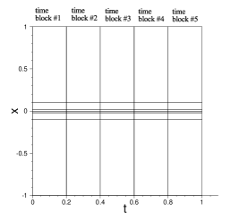
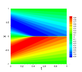
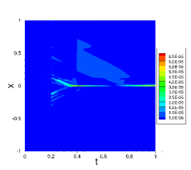
(a) (b) (c)

Figure 20: Burgers’ equation on the larger domain $\Omega$ ($t\in[0,1]$): (a) Configuration of the $5$ uniform time blocks and the $6$ non-uniform sub-domains on each time block. Distributions of (b) the locHLConcELM solution and (c) its absolute error. Local network architecture $[2,300,1]$ on each sub-domain, $Q=21\times 21$ per sub-domain, $\mathbf{R}=2.0$.

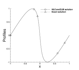
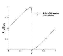
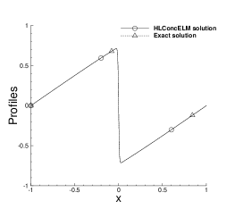
(a) (b) (c)

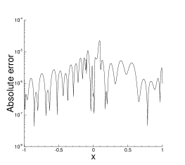
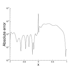
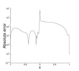
(d) (e) (f)

Figure 21: Burgers’ equation on the larger domain $\Omega$: Profiles of the locHLConcELM solution (top row) and its absolute error (bottom row) at the time instants: $t=0.25$ (a,d), $t=0.5$ (b,e), and $t=1.0$ (c,f). The profiles of the exact solution are also shown in (a,b,c), which overlap with those of the locHLConcELM solution. The locHLConcELM simulation parameters and configurations follow those of Figure 20.

Let us next consider the larger domain $\Omega$ ($t\in[0,1]$) and solve the system (27) using the current method. We employ the locHLConcELM method together with the block time marching scheme (see Remarks 2.5 and 2.6) in the simulation. Specifically, we divide the temporal dimension into $5$ uniform time blocks, and partition each time block into $6$ non-uniform sub-domains along the $x$ direction. Figure 20(a) illustrates the configuration of the time blocks and the sub-domains on each time block, where the $x$ coordinates of the sub-domain boundaries are given by $\bm{\mathcal{X}}=[-1,-0.1,-0.02,0,0.02,0.1,1]$. We employ a local neural network architecture $\mathbf{M}=[2,300,1]$ and a uniform set of $Q=21\times 21$ collocation points on each sub-domain. The hidden magnitude vector is $\mathbf{R}=2.0$, which is obtained using the method of DongY2021 . Figures 20(b) and (c) show the distributions of the locHLConcELM solution and its absolute error on $\Omega$. The data indicate that the current method achieves a quite high accuracy with the sharp gradient present in the domain, with the maximum error on the order of $10^{-5}$.

Figure 21 compares profiles of the locHLConcELM solution and the exact solution (28) for the Burgers’ equation at three time instants $t=0.25$, $0.5$ and $1.0$. The error profiles of the locHLConcELM solution have also been included in this figure. The simulation configuration and the parameters used here correspond to those of Figure 20. It is evident that the current locHLConcELM method has achieved a quite high accuracy for this problem.

3.5 KdV Equation

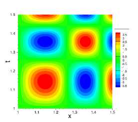
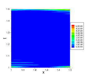
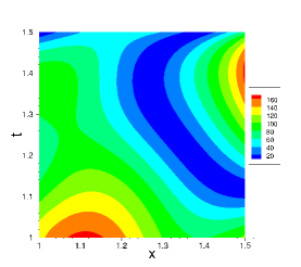
(a) (b) (c)

Figure 22: KdV equation: Distributions of (a) the exact solution, (b) the absolute error of the HLConcELM solution, and (c) the absolute error of the conventional ELM solution. In (b,c), neural network architecture $\mathbf{M}=[2,800,50,1]$, $Q=35\times 35$ uniform collocation points. $\mathbf{R}=(3.2,0.01)$ in (b) for HLConcELM. $R_{m}=R_{m0}=0.27$ in (c) for conventional ELM.

In the next benchmark problem we employ the Korteweg-de Vries (KdV) equation to test the HLConcELM method. Consider the spatial-temporal domain $(x,t)\in\Omega=[1.0,1.5]\times[1.0,1.5]$ and the following initial/boundary value problem,

$$\frac{\partial u}{\partial t}-u\frac{\partial u}{\partial x}+\frac{\partial^{3}u}{\partial x^{3}}=f(x,t),$$ (29a)

$$u(1,t)=g_{1}(t),\quad u(1.5,t)=g_{2}(t),\quad\frac{\partial u}{\partial x}(1,t)=g_{3}(t),$$ (29b)

$$u(x,1)=h(x).$$ (29c)

In the above equations $u(x,t)$ is the field solution to be sought, $f(x,t)$ is a prescribed source term, $g_{i}$ ($i=1,2,3$) and $h$ are the data for the boundary and initial conditions. We choose $f$, $g_{i}$ ($i=1,2,3$) and $h$ such that the system (29) has the following analytic solution,

$$u(x,t)=4\sin\left(\pi x^{3}\right)\sin\left(\pi t^{3}\right).$$ (30)

Figure 23(a) shows the distribution of this solution in the spatial-temporal $xt$ plane.

To solve the problem (29) using the HLConcELM method, we employ neural networks with two input nodes (representing the $x$ and $t$) and a single output node (representing $u$), with the Gaussian activation function for all the hidden nodes. A uniform set of $Q=Q_{1}\times Q_{1}$ collocation points on the domain $\Omega$ is used to train the neural network, where $Q_{1}$ is varied systematically in the tests.

Figures 22(b) and (c) illustrate the absolute-error distributions obtained using the HLConcELM method and the conventional ELM method. Here the network architecture is given by $\mathbf{M}=[2,800,50,1]$, and a uniform set of $Q=35\times 35$ collocation points is used for both methods. The hidden magnitude vector is $\mathbf{R}=(3.2,0.01)$ with HLConcELM, which is obtained using the method of DongY2021 . For conventional ELM, we set the hidden-layer coefficients to random values generated on $[-R_{m},R_{m}]$ with $R_{m}=R_{m0}$, where $R_{m0}=0.27$ is the optimal $R_{m}$ obtained using the method of DongY2021 . The conventional ELM solution is observed to be inaccurate (maximum error on the order of $10^{2}$), because of the narrow last hidden layer in the network. In contrast, the HLConcELM solution is highly accurate, with the maximum error on the order of $10^{-8}$ in the domain.

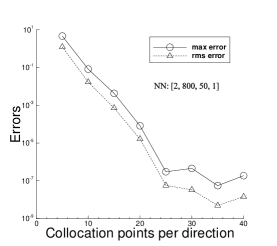
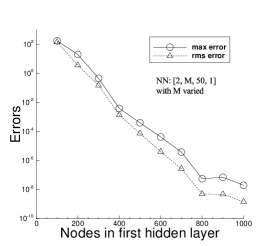
(a) (b)

Figure 23: KdV equation: The HLConcELM maximum/rms errors versus (a) the number of collocation points per direction, and (b) the number of nodes in the first hidden layer ($M$). Network architecture $[2,M,50,1]$. $M=800$ in (a), varied in (b). $Q=35\times 35$ in (b), varied in (a). $\mathbf{R}=(3.2,0.01)$ in (a,b).

Figure 23 illustrates the convergence behavior of the HLConcELM errors with respect to the collocation points and the number of nodes in the network. Here the network architecture is $\mathbf{M}=[2,M,50,1]$, with $M$ either fixed at $M=800$ or varied between $M=100$ and $M=1000$. A uniform set of $Q=Q_{1}\times Q_{1}$ collocation points is used, with $Q_{1}$ either fixed at $Q_{1}=35$ or varied between $Q_{1}=5$ and $Q_{1}=40$. The hidden magnitude vector is $\mathbf{R}=(3.2,0.01)$, obtained from the method of DongY2021 . The two plots (a) and (b) depict the maximum/rms errors of the HLConcELM solution as a function of $Q_{1}$ and $M$, respectively. One can observe the familiar exponential decrease in the errors with increasing $Q_{1}$ or $M$.

neural	collocation	current	ELM	conventional	ELM
network	points	max error	rms error	max error	rms error
$[2,800,50,1]$	$5\times 5$	$4.67E+0$	$1.24E+0$	$1.66E+2$	$8.18E+1$
	$10\times 10$	$8.28E-2$	$1.70E-2$	$1.78E+2$	$1.02E+2$
	$15\times 15$	$4.30E-3$	$7.21E-4$	$1.88E+2$	$9.36E+1$
	$20\times 20$	$8.21E-5$	$1.64E-5$	$1.78E+2$	$9.80E+1$
	$25\times 25$	$3.02E-7$	$5.71E-8$	$1.75E+2$	$8.89E+1$
	$30\times 30$	$4.55E-7$	$3.32E-8$	$1.66E+2$	$7.76E+1$
	$35\times 35$	$5.55E-8$	$4.95E-9$	$1.67E+2$	$7.77E+1$
	$40\times 40$	$1.87E-7$	$1.45E-8$	$1.67E+2$	$7.74E+1$

Table 5: KdV equation: Comparison of the maximum/rms errors from the HLConcELM method and the conventional ELM method. Network architecture: $[2,800,50,1]$. The HLConcELM data in this table correspond to those in Figure 23(a). For conventional ELM, the hidden-layer coefficients are set to uniform random values generated on $[-R_{m},R_{m}]$ with $R_{m}=R_{m0}$. Here $R_{m0}=0.27$ is the optimal $R_{m}$ obtained using the method of DongY2021 .

Table 5 provides an accuracy comparison of the HLConcELM method and the conventional ELM method DongL2021 for solving the KdV equation on a network architecture $\mathbf{M}=[2,800,50,1]$ corresponding to a sequence of collocation points. The HLConcELM solution is highly accurate, while the conventional ELM solution exhibits no accuracy at all on such a neural network.

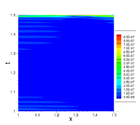
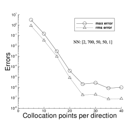
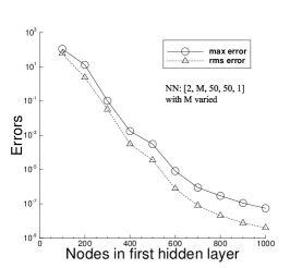
(a) (b) (c)

Figure 24: KdV equation (3 hidden layers in network): (a) Distribution of the absolute error of the HLConcELM solution. The HLConcELM maximum/rms errors versus (b) the number of collocation points per direction, and (c) the number of nodes in the first hidden layer ($M$). Network architecture: $[2,M,50,50,1]$. $M=700$ in (a,b), varied in (c). $Q=35\times 35$ in (a,c), varied in (b). $\mathbf{R}=(3.0,0.025,1.6)$ in (a,b,c).

Figure 24 illustrates the HLConcELM solutions obtained on a deeper neural network with $3$ hidden layers. The neural network architecture is given by $\mathbf{M}=[2,M,50,50,1]$, where $M$ is either fixed at $M=700$ or varied systematically. A hidden magnitude vector $\mathbf{R}=(3.0,0.026,1.6)$ is employed in all the simulations. Figure 24(a) shows the absolute-error distribution on $\Omega$, which corresponds to $M=700$ and a set of $Q=35\times 35$ collocation points. The HLConcELM result is highly accurate, with the maximum error on the order of $10^{-7}$ on $\Omega$. Figures 24(b) and (c) depict the maximum/rms errors of HLConcELM as a function of the number of collocation points and as a function of $M$, respectively. The data again signify the exponential (or near exponential) convergence of the HLConcELM errors.

3.6 Sine-Gordon Equation

(a) (b) (c)

Figure 25: Sine-Gordon equation: Distributions of (a) the exact solution, (b) the absolute error of the HLConcELM solution, and (c) the absolute error of the conventional ELM solution. In (b,c), network architecture $[2,600,30,1]$, Gaussian activation function, $Q=50\times 50$ uniform collocation points. $\mathbf{R}=(1.98,0.23)$ in (b) for HLConcELM. $R_{m}=R_{m0}=1.0$ in (c) for conventional ELM. why are the plots so blurry? image format or vector format in eps? what is the resolution for output? In legend using one decimal point for exponential format.

In the last example we test the HLConcELM method using the nonlinear Sine-Gordon equation. Consider the spatial-temporal domain, $(x,t)\in\Omega=[0,1]\times[0,1]$, and the initial/boundary value problem on $\Omega$,

$$\frac{\partial^{2}u}{\partial t^{2}}-\frac{\partial^{2}u}{\partial x^{2}}+u+\sin(u)=f(x,t),$$ (31a)

$$u(0,t)=g_{1}(t),\quad u(1,t)=g_{2}(t),$$ (31b)

$$u(x,0)=h_{1}(x),\quad\frac{\partial u}{\partial t}(x,0)=h_{2}(x).$$ (31c)

In the above equations, $u(x,t)$ is the field function to be solved for, $f$ is a prescribed source term, and $g_{i}$ and $h_{i}$ ($i=1,2$) are the prescribed boundary and initial data. We choose the source term and the boundary/initial data appropriately such that the problem (31) has the following exact solution,

$$u(x,t)=\left[2\cos\left(2\pi x^{2}\right)+\frac{9}{5}\cos\left(3\pi x+\frac{9}{10}\right)\right]\left[\frac{8}{5}\sin\left(2\pi t^{2}\right)+2\sin\left(\pi x+\frac{4}{5}\right)\right].$$ (32)

Figure 25(a) illustrates the distribution of this solution in the spatial-temporal plane.

To solve the problem (31) by HLConcELM, we employ neural-network architectures having two input nodes (representing $x$ and $t$) and a single output node (representing the solution $u$), with the Gaussian activation function for all the hidden nodes. We train the neural network on a uniform set of $Q=Q_{1}\times Q_{1}$ collocation points, with $Q_{1}$ varied in the tests.

Figures 25(b) and (c) illustrate the absolute-error distributions of the HLConcELM solution and the conventional ELM solution for the Sine-Gordon equation, respectively. For both methods the network architecture is given by $\mathbf{M}=[2,600,30,1]$ and a set of $Q=50\times 50$ collocation points is used. For HLConcELM the hidden magnitude vector is $\mathbf{R}=(1.98,0.23)$, which is obtained using the method of DongY2021 . For conventional ELM, the random hidden-layer coefficients are generated with $R_{m}=R_{m0}=1.0$, which is obtained also with the method of DongY2021 . The conventional ELM solution exhibits no accuracy, with the maximum error on the order of $10$ in the domain (see plot (c)). The HLConcELM solution, on the other hand, is quite accurate, with the maximum error on the order of $10^{-7}$ in the domain.

(a) (b)

Figure 26: Sine-Gordon equation: The HLConcELM maximum/rms errors versus (a) the number of collocation points in each direction, and (b) the number of nodes in the first hidden layer ($M$). Network architecture $[2,M,30,1]$, $Q=Q_{1}\times Q_{1}$ uniform collocation points. $M=600$ in (a), varied in (b). $Q_{1}=50$ in (b), varied in (a). $\mathbf{R}=(1.98,0.23)$ in (a,b). in (a), plot collocation points up to 60 only.

Figure 26 illustrates the convergence behavior of the HLConcELM method for solving the Sine-Gordon equation. The network architecture is $\mathbf{M}=[2,M,30,1]$, with $M$ either fixed at $M=600$ or varied systematically in these tests. A set of $Q=Q_{1}\times Q_{1}$ uniform collocation points is employed, with $Q_{1}$ either fixed at $Q_{1}=50$ or varied systematically. The hidden magnitude vector is $\mathbf{R}=(1.98,0.23)$. The plot (a) shows the HLConcELM errors as a function of $Q_{1}$, corresponding to a fixed $M=600$ in the neural network. The plot (b) shows the HLConcELM errors as a function of $M$, corresponding to a fixed $Q_{1}=50$ for the network training. The exponential convergence of the HLConcELM errors is evident from the data.

(Need table of errors comparing HLConcELM and conventional ELM for [2, 600, 30, 1] for different collocation points.)

(a) (b) (c)

Figure 27: Sine-Gordon equation (3 hidden layers in neural network): (a) HLConcELM absolute-error distribution. The maximum/rms errors of HLConcELM versus (b) the number of collocation points in each direction, and (c) the number of nodes in the first hidden layer ($M$). Network architecture $[2,M,30,30,1]$, $Q=Q_{1}\times Q_{1}$ uniform collocation points. $M=600$ in (a,b), varied in (c). $Q_{1}=50$ in (a,c), varied in (b). $\mathbf{R}=(1.9,0.12,1.5)$ in (a,b,c). Plot (a) too blurry, use a higher resolution for output. in (b), plot collocation points up to 60 only.

Figure 27 is an illustration of the HLConcELM results obtained with three hidden layers in the neural network. Here we employ a network architecture $\mathbf{M}=[2,M,30,30,1]$, with $M$ either fixed at $M=600$ or varied systematically in the tests, and a uniform set of $Q=Q_{1}\times Q_{1}$ collocation points for training the network, with $Q_{1}$ either fixed at $Q_{1}=50$ or varied systematically. The hidden magnitude vector is $\mathbf{R}=(1.9,0.12,1.5)$, which is obtained using the method from DongY2021 . Figure 27(a) shows the absolute-error distribution of the HLConcELM solution in the spatial-temporal plane, corresponding to $M=600$ and $Q_{1}=50$ in the simulation. The HLConcELM method produces an accurate solution, with the maximum error on the order of $10^{-7}$ in the domain. Figures 27(b) and (c) depict the maximum/rms errors of HLConcELM as a function of $Q_{1}$ and $M$, respectively. It is evident that these errors decrease exponentially (before saturation) with increasing collocation points or hidden nodes in the neural network.

4 Concluding Remarks

The extreme learning machine (ELM) method can yield highly accurate solutions to linear and nonlinear PDEs. In terms of the accuracy and computational cost, it exhibits a notable advantage over the existing DNN-based PDE solvers and the the traditional numerical methods such as the second-order and high-order finite element methods (see DongL2021 ; DongY2021 ). To achieve a high accuracy, the existing ELM method DongL2021 ; DongL2021bip ; DongY2021 requires the last hidden layer of the neural network to be wide. So the ELM neural network typically contains a large number of nodes in the last hidden layer, irrespective of the rest of network configuration. If the last hidden layer is narrow, the ELM accuracy will suffer and tend to be poor, even though the neural network may contain a large number of the nodes in the other hidden layers.

In the current paper we have presented a method to overcome the above drawback of the existing (conventional) ELM method. The new method, termed HLConcELM (hidden-layer concatenated ELM), can produce highly accurate solutions to linear/nonlinear PDEs when the last hidden layer is wide, and when the last hidden layer is narrow, in which case the conventional ELM completely losses accuracy.

The new method relies on a type of modified feedforward neural networks (FNN), which exposes the hidden nodes in all the hidden layers to the output nodes by incorporating a logical concatenation of the hidden layers into the network. We refer to this modified network as HLConcFNN (hidden-layer concatenated FNN) in this paper. In HLConcFNN every hidden node in the network directly influences the nodes in the output layer, while in conventional FNN only the hidden nodes in the last hidden layer directly influence the output nodes. HLConcFNNs have the interesting property that, if new hidden layers are appended to an existing network architecture or new nodes are added to an existing hidden layer, the representation capacity of the resultant network architecture is guaranteed to be not smaller than that of the original one.

The HLConcELM method adopts the HLConcFNN as its neural network. It assigns random values to (and fixes) the weight/bias coefficients in all the hidden layers of the neural network, while the coefficients between the output nodes and all the hidden nodes of the network are trained/computed by a linear or nonlinear least squares method. Note that in HLConcELM every hidden node in the network is connected to the output nodes because of the logical hidden-layer concatenation. HLConcELMs have the property that, as new hidden layers are appended to an existing network architecture, the representation capacity of the HLConcELM associated with the resultant architecture is guaranteed to be not smaller than that associated with the original one, provided that the random coefficients in the resultant architecture are assigned in an appropriate fashion.

In essence, when solving PDEs or approximating functions, the ELM method performs an expansion of the unknown field solution in terms of a set of random basis functions. With conventional ELM, the random bases consist of the output fields of the last hidden layer of the neural network. With HLConcELM, on the other hand, the random bases consist of the output fields of the hidden nodes in all the hidden layers of the neural network. HLConcELM is able to harvest the degrees of freedom provided by all the hidden nodes in the network, not limited to those from the last hidden layer. This is the essential difference between the HLConcELM method and the conventional ELM method.

We have tested the current HLConcELM method on boundary value problems and initial/boundary value problems involving a number of linear and nonlinear PDEs. In particular, we have compared HLConcELM and the conventional ELM on network architectures whose last hidden layer is narrow or wide. The numerical results demonstrate that the current HLConcELM method yields highly accurate results on network architectures with both narrow and wide last hidden layers. In contrast, the conventional ELM only achieves accurate results on architectures with a wide last hidden layer, and with a narrow last hidden layer it exhibits poor or no accuracy. The HLConcELM method displays an exponentially convergent behavior for smooth field solutions, reminiscent of the traditional high-order techniques KarniadakisS2005 ; ZhengD2011 ; YangD2020 ; YangLD2019 ; YangD2019 . Its numerical errors decrease exponentially or nearly exponentially as the number of collocation points or the number of trainable parameters increases.

Appendix A: Proofs of Theorems from Section 2

Proof of Theorem 2.1:

Proof.

Consider an arbitrary $u(\bm{\theta},\bm{\beta},\mathbf{x})\in U(\Omega,\mathbf{M}_{1},\sigma)$, where $\bm{\theta}\in\mathbb{R}^{N_{h1}}$ and $\bm{\beta}\in\mathbb{R}^{N_{c1}}$, with $N_{h1}=\sum_{i=1}^{L-1}(m_{i-1}+1)m_{i}$ and $N_{c1}=\sum_{i=1}^{L-1}m_{i}$. Let $w_{kj}^{(i)}$ ($1\leqslant i\leqslant L-1$, $1\leqslant k\leqslant m_{i-1}$, $1\leqslant j\leqslant m_{i}$) and $b^{(i)}_{j}$ ($1\leqslant i\leqslant L-1$, $1\leqslant j\leqslant m_{i}$) denote the hidden-layer weight/bias coefficients of the associated HLConcFNN($\mathbf{M}_{1},\sigma$), and let $\beta_{ij}$ ($1\leqslant i\leqslant L-1$, $1\leqslant j\leqslant m_{i}$) denote the output-layer coefficients of HLConcFNN($\mathbf{M}_{1},\sigma$). $u(\bm{\theta},\bm{\beta},\mathbf{x})$ is given by (7).

Consider a function $v(\bm{\vartheta},\bm{\alpha},\mathbf{x})\in U(\Omega,\mathbf{M}_{2},\sigma)$ with $\bm{\vartheta}\in\mathbb{R}^{N_{h2}}$ and $\bm{\alpha}\in\mathbb{R}^{N_{c2}}$, where $N_{c2}=N_{c1}+n$, and $N_{h2}=N_{h1}+(m_{L-1}+1)n$. We will choose $\bm{\vartheta}$ and $\bm{\alpha}$ such that $v(\bm{\vartheta},\bm{\alpha},\mathbf{x})=u(\bm{\theta},\bm{\beta},\mathbf{x})$. We construct $\bm{\vartheta}$ and $\bm{\alpha}$ by setting the hidden-layer and the output-layer coefficients of HLConcFNN($\mathbf{M}_{2},\sigma$) as follows.

The HLConcFNN($\mathbf{M}_{2},\sigma$) has $L$ hidden layers. We set the weight/bias coefficients in its last hidden layer (with $n$ nodes) to arbitrary values. We set those coefficients that connect the output node and the $n$ nodes in the last hidden layer to all zeros. For the rest of the hidden-layer coefficients and the output-layer coefficients in HLConcFNN($\mathbf{M}_{2},\sigma$), we use those corresponding coefficient values from the network HLConcFNN($\mathbf{M}_{1},\sigma$).

More specifically, let $\xi_{kj}^{(i)}$ and $\eta_{j}^{(i)}$ denote the weight/bias coefficients in the hidden layers, and $\alpha_{ij}$ denote the output-layer coefficients, of HLConcFNN($\mathbf{M}_{2},\sigma$) associated with the function $v(\bm{\vartheta},\bm{\alpha},\mathbf{x})$. We set these coefficients by,

$$\xi_{kj}^{(i)}=\left\{\begin{array}[]{ll}w_{kj}^{(i)},&\text{for}\ 1\leqslant i\leqslant L-1,\ 1\leqslant k\leqslant m_{i-1},\ 1\leqslant j\leqslant m_{i};\\ \text{arbitrary value},&\text{for}\ i=L,\ 1\leqslant k\leqslant m_{L-1},\ 1\leqslant j\leqslant n;\end{array}\right.$$ (33)

$$\eta_{j}^{(i)}=\left\{\begin{array}[]{ll}b_{j}^{(i)},&\text{for all}\ 1\leqslant i\leqslant L-1,\ 1\leqslant j\leqslant m_{i};\\ \text{arbitrary value},&\text{for}\ i=L,\ 1\leqslant j\leqslant n;\end{array}\right.$$ (34)

$$\alpha_{ij}=\left\{\begin{array}[]{ll}\beta_{ij},&\text{for}\ 1\leqslant i\leqslant L-1,\ 1\leqslant j\leqslant m_{i};\\ 0,&\text{for}\ i=L,\ 1\leqslant j\leqslant n.\end{array}\right.$$ (35)

With the above coefficients, the last hidden layer of the network HLConcFNN($\mathbf{M}_{2},\sigma$) may output arbitrary fields, which however have no effect on the output field of HLConcFNN($\mathbf{M}_{2},\sigma$) because $\alpha_{Lj}=0$ ($1\leqslant j\leqslant n$). The rest of the hidden nodes in HLConcFNN($\mathbf{M}_{2},\sigma$) and the output node of HLConcFNN($\mathbf{M}_{2},\sigma$) produce fields that are identical to those of the corresponding nodes in the network HLConcFNN($\mathbf{M}_{1},\sigma$). We thus conclude that $u(\bm{\theta},\bm{\beta},\mathbf{x})=v(\bm{\vartheta},\bm{\alpha},\mathbf{x})$. So $u(\bm{\theta},\bm{\beta},\mathbf{x})\in U(\Omega,\mathbf{M}_{2},\sigma)$, and the relation (9) holds. ∎

Proof of Theorem 2.2:

Proof.

We use the same strategy as that in the proof of Theorem 2.1. Consider an arbitrary $u(\bm{\theta},\bm{\beta},\mathbf{x})\in U(\Omega,\mathbf{M}_{1},\sigma)$, where $\bm{\theta}\in\mathbb{R}^{N_{h1}}$ and $\bm{\beta}\in\mathbb{R}^{N_{c1}}$, with $N_{h1}=\sum_{i=1}^{L-1}(m_{i-1}+1)m_{i}$ and $N_{c1}=\sum_{i=1}^{L-1}m_{i}$. The hidden-layer coefficients of the associated HLConcFNN($\mathbf{M}_{1},\sigma$) are denoted by $w_{kj}^{(i)}$ ($1\leqslant i\leqslant L-1$, $1\leqslant k\leqslant m_{i-1}$, $1\leqslant j\leqslant m_{i}$) and $b^{(i)}_{j}$ ($1\leqslant i\leqslant L-1$, $1\leqslant j\leqslant m_{i}$), and the output-layer coefficients are denoted by $\beta_{ij}$ ($1\leqslant i\leqslant L-1$, $1\leqslant j\leqslant m_{i}$). $u(\bm{\theta},\bm{\beta},\mathbf{x})$ is given by (7).

Consider a function $v(\bm{\vartheta},\bm{\alpha},\mathbf{x})\in U(\Omega,\mathbf{M}_{2},\sigma)$ with $\bm{\vartheta}\in\mathbb{R}^{N_{h2}}$ and $\bm{\alpha}\in\mathbb{R}^{N_{c2}}$, where $N_{c2}=N_{c1}+1$, and $N_{h2}=N_{h1}+(m_{s-1}+1)+m_{s+1}$ if $1\leqslant s\leqslant L-2$ and $N_{h2}=N_{h1}+(m_{s-1}+1)$ if $s=L-1$. We construct $\bm{\vartheta}$ and $\bm{\alpha}$ by setting the hidden-layer and the output-layer coefficients of HLConcFNN($\mathbf{M}_{2},\sigma$) as follows.

In HLConcFNN($\mathbf{M}_{2},\sigma$) we set the weight coefficients that connect the extra node of layer $s$ to those nodes in layer $(s+1)$ to all zeros, and we also set the weight coefficient that connects the extra node of layer $s$ with the output node to zero. We set the weight coefficients that connect the nodes of layer $(s-1)$ to the extra node of layer $s$ to arbitrary values, and also set the bias coefficient corresponding to the extra node of layer $s$ to an arbitrary value. For the rest of the hidden-layer and output-layer coefficients of HLConcFNN($\mathbf{M}_{2},\sigma$), we use those corresponding coefficient values from the network HLConcFNN($\mathbf{M}_{1},\sigma$).

Specifically, let $\xi_{kj}^{(i)}$ and $\eta_{j}^{(i)}$ denote the weight/bias coefficients in the hidden layers, and $\alpha_{ij}$ denote the output-layer coefficients, of the HLConcFNN($\mathbf{M}_{2},\sigma$) associated with $v(\bm{\vartheta},\bm{\alpha},\mathbf{x})$. We set these coefficients by,

$$\xi_{kj}^{(i)}=\left\{\begin{array}[]{ll}w_{kj}^{(i)},&\text{for all}\ (1\leqslant i\leqslant s-1,\ \text{or}\ s+2\leqslant i\leqslant L-1),\ 1\leqslant k\leqslant m_{i-1},\ 1\leqslant j\leqslant m_{i};\\ w_{kj}^{(s)},&\text{for}\ i=s,\ 1\leqslant k\leqslant m_{s-1},\ 1\leqslant j\leqslant m_{s};\\ \text{arbitrary value},&\text{for}\ i=s,\ 1\leqslant k\leqslant m_{s-1},\ j=m_{s}+1;\\ w_{kj}^{(s+1)},&\text{for}\ i=s+1,\ 1\leqslant k\leqslant m_{s},\ 1\leqslant j\leqslant m_{s+1};\\ 0,&\text{for}\ i=s+1,\ k=m_{s}+1,\ 1\leqslant j\leqslant m_{s+1};\end{array}\right.$$ (36)

$$\eta_{j}^{(i)}=\left\{\begin{array}[]{ll}b_{j}^{(i)},&\text{for all}\ 1\leqslant i\leqslant L-1,\ i\neq s,\ 1\leqslant j\leqslant m_{i};\\ b_{j}^{(s)},&\text{for}\ i=s,\ 1\leqslant j\leqslant m_{s};\\ \text{arbitrary value},&\text{for}\ i=s,\ j=m_{s}+1;\end{array}\right.$$ (37)

$$\alpha_{ij}=\left\{\begin{array}[]{ll}\beta_{ij},&\text{for all}\ 1\leqslant i\leqslant L-1,\ i\neq s,\ 1\leqslant j\leqslant m_{i};\\ \beta_{sj},&\text{for}\ i=s,\ 1\leqslant j\leqslant m_{s};\\ 0,&\text{for}\ i=s,\ j=m_{s}+1.\end{array}\right.$$ (38)

With the above coefficients, the extra node in layer $s$ of the network HLConcFNN($\mathbf{M}_{2},\sigma$) may output an arbitrary field, which however has no contribution to the output field of HLConcFNN($\mathbf{M}_{2},\sigma$). The rest of the hidden nodes and the output node of HLConcFNN($\mathbf{M}_{2},\sigma$) produce identical fields as the corresponding nodes in the network HLConcFNN($\mathbf{M}_{1},\sigma$). We thus conclude that $u(\bm{\theta},\bm{\beta},\mathbf{x})=v(\bm{\vartheta},\bm{\alpha},\mathbf{x})$. So $u(\bm{\theta},\bm{\beta},\mathbf{x})\in U(\Omega,\mathbf{M}_{2},\sigma)$ and the relation (10) holds. ∎

References

- [1] P.A. Alaba, S.I. Popoola, L. Olatomiwa, M.B. Akanle, O.S. Ohunakin, E. Adetiba, O.D. Alex, A.A.A. Atayero, and W.M.A.W. Daud. Towards a more efficient and cost-sensitive extreme learning machine: a state-of-the-art review of recent trend. Neurocomputing, 350:70–90, 2019.
- [2] C. Basdevant, M. Deville, P. Haldenwang, J.M. Lacroix, J. Ouazzani, R. Peyret, P. Orlandi, and A.T. Patera. Spectral and finite difference solutions of the Burgers equation. Computers and Fluids, 14:23–41, 1986.
- [3] H.A.T. Braake and G.V. Straten. Random activation weight neural net (RAWN) for fast non-iterative training. Eng. Applic. Artif. Intell., 8:71–80, 1995.
- [4] M.A. Branch, T.F. Coleman, and Y. Li. A subspace, interior, and conjugate gradient method for large-scale bound-constrained minimization problems. SIAM Journal on Scientific Computing, 21:1–23, 1999.
- [5] R.H. Byrd, R.B. Schnabel, and G.A. Shultz. Approximate solution of the trust region problem by minimization over two-dimensional subspaces. Math. Programming, 1988.
- [6] F. Calabro, G. Fabiani, and C. Siettos. Extreme learning machine collocation for the numerical solution of elliptic PDEs with sharp gradients. Computer Methods in Applied Mechanics and Engineering, 387:114188, 2021.
- [7] C. Cortes, X. Gonzalvo, V. Kuznetsov, M. Mohri, and S. Yang. Adanet: Adaptive structural learning of artificial neural networks. arXiv:1607.01097, 2016.
- [8] E.C. Cyr, M.A. Gulian, R.G. Patel, M. Perego, and N.A. Trask. Robust training and initialization of deep neural networks: An adaptive basis viewpoint. Proceedings of Machine Learning Research, 107:512–536, 2020.
- [9] S. Dong and Z. Li. Local extreme learning machines and domain decomposition for solving linear and nonlinear partial differential equations. Computer Methods in Applied Mechanics and Engineering, 387:114129, 2021. (also arXiv:2012.02895).
- [10] S. Dong and Z. Li. A modified batch intrinsic plascity method for pre-training the random coefficients of extreme learning machines. Journal of Computational Physics, 445:110585, 2021. (also arXiv:2103.08042).
- [11] S. Dong and N. Ni. A method for representing periodic functions and enforcing exactly periodic boundary conditions with deep neural networks. Journal of Computational Physics, 435:110242, 2021.
- [12] S. Dong and J. Yang. On computing the hyperparameter of extreme learning machines: algorithms and applications to computational PDEs, and comparison with classical and high-order finite elements. arXiv:2110.14121, 2021.
- [13] S. Dong and J. Yang. Numerical approximation of partial differential equations by a variable projection method with artificial neural networks. arXiv:2201.09989, 2022.
- [14] V. Dwivedi and B. Srinivasan. Physics informed extreme learning machine (pielm) a rapid method for the numerical solution of partial differential equations. Neurocomputing, 391:96–118, 2020.
- [15] V. Dwivedi and B. Srinivasan. A normal equation-based extreme learning machine for solving linear partial differential equations. Journal of Computing and Information Science in Engineering, 22:014502, 2022.
- [16] W. E and B. Yu. The deep Ritz method: a deep learning-based numerical algorithm for solving variational problems. Communications in Mathematics and Statistics, 6:1–12, 2018.
- [17] G. Fabiani, F. Calabro, L. Russo, and C. Siettos. Numerical solution and bifurcation analysis of nonlinear partial differential equations with extreme learning machines. Journal of Scientific Computing, 89:44, 2021.
- [18] A.L. Freire, A.R. Rocha-Neto, and G.A. Barreto. On robust randomized neural networks for regression: a comprehensive review and evaluation. Neural Computing and Applications, 32:16931–16950, 2020.
- [19] E. Galaris, G. Fabiani, F. Calabro, D.d. Serafino, and C. Siettos. Numerical solution of stiff ODEs with physics-informed random projection neural networks. arXiv:2108.01584, 2021.
- [20] I. Goodfellow, Y. Bengio, and A. Courville. Deep Learning. The MIT Press, 2016.
- [21] P. Guo, C.P. Chen, and Y. Sun. An exact supervised learning for a three-layer supervised neural network. In Proceedings of 1995 International Conference on Neural Information Processing, pages 1041–1044, 1995.
- [22] J. He and J. Xu. MgNet: A unified framework for multigrid and convolutional neural network. Science China Mathematics, 62:1331–1354, 2019.
- [23] G. Huang, G.B. Huang, S. Song, and K. You. Trends in extreme learning machines: a review. Neural Networks, 61:32–48, 2015.
- [24] G. Huang, Z. Liu, L. van der Maaten, and K.Q. Weinberger. Densely connected convolutional networks. arXiv:1608.06993, 2018.
- [25] G.-B. Huang, Q.-Y. Zhu, and C.-K. Siew. Extreme learning machine: a new learning scheme of feedforward neural networks. In 2004 IEEE International Joint Conference on Neural Networks, volume 2, pages 985–990, 2004.
- [26] G.-B. Huang, Q.-Y. Zhu, and C.-K. Siew. Extreme learning machine: theory and applications. Neurocomputing, 70:489–501, 2006.
- [27] G.B. Huang, L. Chen, and C.-K. Siew. Universal approximation using incremental constructive feedforward networks with random hidden nodes. IEEE Transactions on Neural Networks, 17:879–892, 2006.
- [28] B. Igelnik and Y.H. Pao. Stochastic choice of basis functions in adaptive function approximation and the functional-link net. IEEE Transactions on Neural Networks, 6:1320–1329, 1995.
- [29] H. Jaeger, M. Lukosevicius, D. Popovici, and U. Siewert. Optimization and applications of echo state networks with leaky integrator neurons. Neural Networks, 20:335–352, 2007.
- [30] A.D. Jagtap, E. Kharazmi, and G.E. Karniadakis. Conservative physics-informed neural networks on discrete domains for conservation laws: applications to forward and inverse problems. Computer Methods in Applied Mechanics and Engineering, 365:113028, 2020.
- [31] G.E. Karniadakis, G. Kevrekidis, L. Lu, P. Perdikaris, S. Wang, and L. Yang. Physics-informed machine learning. Nature Reviews Physics, 3:422–440, 2021.
- [32] G.E. Karniadakis and S.J. Sherwin. Spectral/hp element methods for computational fluid dynamics, 2nd edn. Oxford University Press, 2005.
- [33] R. Katuwal, P.N. Suganthan, and M. Tanveer. Random vector functional link neural network based ensemble deep learning. arXiv:1907.00350, 2019.
- [34] A.S. Krishnapriyan, A. Gholami, S. Zhe, R.M. Kirby, and M.W. Mahoney. Characterizing possible failure modes in physics-informed neural networks. arXiv:2109.01050, 2021.
- [35] J.-Y. Li, W. Chow, B. Igelnik, and Y.-H. Pao. Comments on “stochastic choice of basis functions in adaptive function approximaton and the functional-link net”. IEEE Trans. Neural Netw., 8:452–454, 1997.
- [36] H. Liu, B. Xing, Z. Wang, and L. Li. Legendre neural network method for several classes of singularly perturbed differential equations based on mapping and piecewise optimization technology. Neural Processing Letters, 51:2891–2913, 2020.
- [37] M. Liu, M. Hou, J. Wang, and Y. Cheng. Solving two-dimensional linear partial differential equations based on Chebyshev neural network with extreme learning machine algorithm. Engineering Computations, 38:874–894, 2021.
- [38] L. Lu, X. Meng, Z. Mao, and G.E. Karniadakis. DeepXDE: a deep learning library for solving differential equations. SIAM Review, 63:208–228, 2021.
- [39] M. Lukosevicius and H. Jaeger. Reservoir computing approaches to recurrent neural network training. Comput. Sci. Rev., 3:127–149, 2009.
- [40] W. Maas and H. Markram. On the computational power of recurrent circuits of spiking neurons. J. Comput. Syst. Sci., 69:593–616, 2004.
- [41] D. Needell, A.A. Nelson, R. Saab, and P. Salanevich. Random vector functional link networks for function approximation on manifolds. arXiv:2007.15776, 2020.
- [42] J. Nocedal and S.J. Wright. Numerical Optimization, Second Edition. Springer, 2006.
- [43] S. Panghal and M. Kumar. Optimization free neural network approach for solving ordinary and partial differential equations. Engineering with Computers, 37:2989–3002, 2021.
- [44] Y.H. Pao, G.H. Park, and D.J. Sobajic. Learning and generalization characteristics of the random vector functional-link net. Neurocomputing, 6:163–180, 1994.
- [45] Y.H. Pao and Y. Takefuji. Functional-link net computing: theory, system architecture, and functionalities. Computer, 25:76–79, 1992.
- [46] A. Rahimi and B. Recht. Weighted sums of random kitchen sinks: Replacing minimization with randomization in learning. In D. Koller, D. Schuurmans, Y. Bengio and L. Bottou, editors, Advances in Neural Information Processing Systems (NIPS), 2:1316–1323, 2008.
- [47] M. Raissi, P. Perdikaris, and G.E. Karniadakis. Physics-informed neural networks: a deep learning framework for solving forward and inverse problems involving nonlinear partial differential equations. Journal of Computational Physics, 378:686–707, 2019.
- [48] F. Rosenblatt. The perceptron: a probabilistic model for information storage and organization in the brain. Psychol. Rev., 65:386–408, 1958.
- [49] S. Scardapane and D. Wang. Randomness in neural networks: an overview. WIREs Data Mining Knowl. Discov., 7:e1200, 2017.
- [50] J. Sirignano and K. Spoliopoulos. DGM: A deep learning algorithm for solving partial differential equations. Journal of Computational Physics, 375:1339–1364, 2018.
- [51] P.N. Suhanthan and R. Katuwal. On the origins of randomization-based feedforward neural networks. Applied Soft Computing, 105:107239, 2021.
- [52] H. Sun, M. Hou, Y. Yang, T. Zhang, F. Weng, and F. Han. Solving partial differential equations based on bernsteirn neural network and extreme learning machine algorithm. Neural Processing Letters, 50:1153–1172, 2019.
- [53] K. Tang, X. Wan, and Q. Liao. Adaptive deep density estimation for fokker-planck equations. Journal of Computational Physics, 457:111080, 2022.
- [54] B.K. Verma and J.J. Mulawka. A modified backpropagation algorithm. In Proceedings of 1994 IEEE International Conference on Neural Networks, volume 2, pages 840–844, 1994.
- [55] X. Wan and S. Wei. VAE-KRnet and its applications to variational Bayes. Communications in Computational Physics, in press, 2021. arXiv:2006.16431.
- [56] S. Wang, X. Yu, and P. Perdikaris. When and why PINNs fail to train: a neural tangent kernel perspective. Journal of Computational Physics, 449:110768, 2022.
- [57] Y. Wang and G. Lin. Efficient deep learning techniques for multiphase flow simulation in heterogeneous porous media. Journal of Computational Physics, 401:108968, 2020.
- [58] C.S. Webster. Alan Turing’s unorganized machines and artificial neural networks: his remarkable early work and future possibilities. Evol. Intel., 5:35–43, 2012.
- [59] B. Widrow, A. Greenblatt, Y. Kim, and D. Park. The no-prop algorithm: a new learning algorithm for multilayer neural networks. Neural Networks, 37:182–188, 2013.
- [60] B.M. Wilamowski and H. Yu. Neural network learning without backpropagation. IEEE Transactions on Neural Networks, 21:1793–1803, 2010.
- [61] N. Winovich, K. Ramani, and G. Lin. ConvPDE-UQ: Convolutional neural networks with quantified uncertainty for heterogeneous elliptic partial differential equations on varied domains. Journal of Computational Physics, 394:263–279, 2019.
- [62] Y. Yang, M. Hou, and J. Luo. A novel improved extreme learning machine algorithm in solving ordinary differential equations by legendre neural network methods. Advances in Differential Equations, 469:1–24, 2018.
- [63] Z. Yang and S. Dong. An unconditionally energy-stable scheme based on an implicit auxiliary energy variable for incompressible two-phase flows with different densities involving only precomputable coefficient matrices. Journal of Computational Physics, pages 229–257, 2019.
- [64] Z. Yang and S. Dong. A roadmap for discretely energy-stable schemes for dissipative systems based on a generalized auxiliary variable with guaranteed positivity. Journal of Computational Physics, 404:109121, 2020. (also arXiv:1904.00141).
- [65] Z. Yang, L. Lin, and S. Dong. A family of second-order energy-stable schemes for Cahn-Hilliard type equations. Journal of Computational Physics, 383:24–54, 2019.
- [66] L. Zhang and P.N. Suganthan. A comprehensive evaluation of random vector functional link networks. Inf. Sci., 367–368:1094–1105, 2016.
- [67] X. Zheng and S. Dong. An eigen-based high-order expansion basis for structured spectral elements. Journal of Computational Physics, 230:8573–8602, 2011.