Thermal Evolution of Dirac Magnons in the Honeycomb Ferromagnet CrBr₃

Abstract

CrBr₃ is an excellent realization of the two-dimensional honeycomb ferromagnet, which offers a bosonic equivalent of graphene with Dirac magnons and topological character. We perform inelastic neutron scattering (INS) measurements using state-of-the-art instrumentation to update 50-year-old data, thereby enabling a definitive comparison both with recent experimental claims of a significant gap at the Dirac point and with theoretical predictions for thermal magnon renormalization. We demonstrate that CrBr₃ has next-neighbor $J_{2}$ and $J_{3}$ interactions approximately 5% of $J_{1}$, an ideal Dirac magnon dispersion at the K point, and the associated signature of isospin winding. The magnon lifetime and the thermal band renormalization show the universal $T^{2}$ evolution expected from an interacting spin-wave treatment, but the measured dispersion lacks the predicted van Hove features, highlighting the need for a deeper theoretical analysis.

Graphene, the original two-dimensional (2D) material, is a single layer of carbon atoms with strong covalent bonds forming a honeycomb lattice, and some of its exceptional physical properties Novoselov et al. (2004, 2005); Geim (2009) are a consequence of its band-structure topology, which allows the electrons to behave as massless quasiparticles described by the Dirac equation. The same band structure is realized for bosonic quasiparticles in systems such as a 2D ferromagnet (FM) on the honeycomb lattice Pershoguba et al. (2018) shown in Fig. 1(a), which has magnon excitations that also exhibit Dirac cones at the K points of the Brillouin zone (BZ), as represented in Fig. 1(b). The topology of magnon band structures has became a matter of active theoretical Li et al. (2017); Pershoguba et al. (2018); McClarty (2022); Mook et al. (2021) and experimental Yao et al. (2018); Chen et al. (2018); Yuan et al. (2020); Elliot et al. (2021); Cai et al. (2021); Scheie et al. (2022) research due to possible applications in spintronic devices Chumak et al. (2015); Wang et al. (2018); Pirro et al. (2021). Inelastic neutron scattering (INS) provides direct access to the magnon dispersion, and the spectra of a number of honeycomb FMs have been measured in their low-temperature regimes ($T\ll\ T_{c}$, the temperature of magnetic order) Chen et al. (2018); Elliot et al. (2021); Chen et al. (2021).

Promising materials for these studies are the family of chromium trihalides, Cr$X_{3}$ ($X=$ Cl Morosin and Narath (1964), Br Samuelsen et al. (1971), I McGuire et al. (2015)), in which the honeycomb layers [Fig. 1(a)] have identical stacking, but $T_{c}$, the size, and even the sign of the interlayer magnetic interaction all vary with $X$ Wang et al. (2011). Measurements on CrCl₃ Chen et al. (2021); Do et al. (2022) indicate a Dirac-cone magnon dispersion [Fig. 1(b)], but in CrI₃ a gap is reported Chen et al. (2018) at the K point, creating acoustic and optical magnon modes [Fig. 1(c)] whose anticrossing is thought to be a consequence of strong next-neighbor Dzyaloshinskii-Moriya (DM) interactions. CrBr₃ was for 50 years considered as a textbook example of FM magnons, with no indication for a band splitting Samuelsen et al. (1971); Yelon and Silberglitt (1971), but the recent report of a large, DM-induced anticrossing Cai et al. (2021) similar to CrI₃ has created controversy. Theoretical calculations based on a Dirac-cone spectrum have predicted a very specific $T^{2}$ form for the temperature-induced renormalization of the magnon dispersion and line width Pershoguba et al. (2018), and cited the old INS results as verification, but systematic measurements of the thermal evolution of the magnon spectrum remain absent.

In this Letter we perform a comprehensive study of the temperature-induced renormalization of the magnon self-energy in CrBr₃ using modern neutron spectrometers. We first use low-temperature INS data to refine the magnetic spin Hamiltonian and find weak next-neighbor interactions. We prove that the magnon dispersion has Dirac cones, the recent report to the contrary apparently being an artifact of the data treatment, and we demonstrate near-ideal cosinusoidal intensity winding around the K points. Working at temperatures up to 40 K, we find considerable downward renormalization of the magnon dispersion and growing line widths, whose $T^{2}$ form we characterize to high accuracy, but the variation of these terms across the BZ is not well captured by the available theory. Our results set the experimental standard for temperature-induced modification of the spin dynamics in a honeycomb ferromagnet.

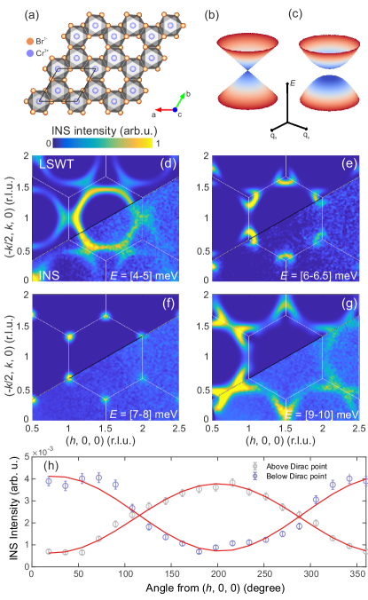
Figure 1: (a) Honeycomb layer of CrBr₃. The Cr³⁺ ions (blue) host $S=3/2$ spins with FM interactions. (b,c) Schematic spin-wave spectra in the vicinity of the K points. When inversion symmetry is preserved, $\omega_{q}\propto q$ and the dispersion forms a Dirac cone (b); otherwise a gap opens to form separate acoustic and optical magnon branches (c). (d-g) Scattered intensity obtained by integrating the PANTHER $E_{\mathrm{i}}=30$ meV dataset over four constant-energy windows (indicated) and compared with linear spin-wave theory (LSWT); all panels have the same intensity scale. White lines indicate the boundaries of the crystallographic BZ. A $\mathbf{Q}$-independent background was subtracted from each spectrum to aid visual comparison. (h) Intensity obtained by winding around the K point, showing a cosinusoidal modulation with inverted phase for energies above and below the Dirac point.

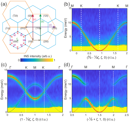
Figure 2: Low-temperature magnon dispersion measured along several high-symmetry directions. (a) Reciprocal-space representation of the honeycomb lattice in the $(h\,k\,0)$ plane showing the crystallographic BZ in blue and the unfolded zone in orange. Green, red, and violet arrows indicate the paths for the spectra shown respectively in panels (b), (c), and (d); the gray arrow indicates the complete path used in Fig. 3. (b-d) Spin-wave spectra collected using PANTHER with $E_{\mathrm{i}}=30$ meV at $T=1.7$ K. The data were integrated by $\pm 0.03$ r.l.u. along the orthogonal in-plane direction and $\pm 5$ r.l.u. in the out-of-plane $l$ direction. Red and green points show respectively the dispersions of modes 1 and 2 modelled by LSWT and their sizes represent the calculated intensities.

Experiment. A 1.5 g single crystal of CrBr₃ was grown by slow sublimation in a temperature gradient under vacuum, as detailed in Sec. S1 of the Supplementary Materials (SM) SI . Its high quality was confirmed by single-crystal neutron diffraction, from which we determined the lattice parameters at 1.7 K as $a=b=6.31$ Å and $c=18.34$ Å, and confirmed the BiI₃-type structure with space group R${\overline{3}}$. We conducted two INS experiments, using the time-of-flight (TOF) spectrometer PANTHER at the Institut Laue-Langevin pan ; Nikitin et al. (2021) and the triple-axis spectrometer (TAS) EIGER at the Paul Scherrer Institute Stuhr et al. (2017). In both experiments the sample was oriented in the $(h\,k\,0)$ scattering plane. On PANTHER we collected data at $T=1.7$, 20, 30, and 40 K, each with two incident neutron energies, $E_{\mathrm{i}}=15$ and 30 meV, and performed TOF data reduction and analysis using the software MANTID Arnold et al. (2014) and HORACE Ewings et al. (2016). On EIGER we used the fixed-$k_{\mathrm{f}}$ mode and worked at eight different temperatures from 1.5 to 40 K. Calculations of the low-temperature magnon dispersion and intensity, which we used to fit the spin Hamiltonian, were performed using the SpinW package Toth and Lake (2015).

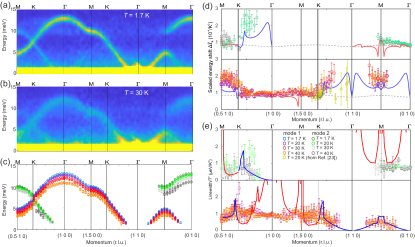
Figure 3: Thermal magnon renormalization in CrBr₃. (a,b) Magnon spectra for the high-symmetry directions taken from the PANTHER $E_{\mathrm{i}}=30$ meV dataset at $T=1.7$ K (a) and $T=30$ K (b). The data were integrated over $\pm 0.015$ Å^-1 in-plane and $\pm 2$ Å^-1 for $l$. (c) Magnon branches 1 and 2 extracted for the four experimental temperatures; circles were taken from the $E_{\mathrm{i}}=30$ meV dataset and squares from $E_{\mathrm{i}}=15$ meV. The mode intensities vanish in some regions of the unfolded BZ. (d) Temperature-induced renormalization of the measured magnon dispersions for modes 1 (upper) and 2 (lower panel), shown in the reduced form of Eq. (2). Solid lines show the real part of the self-energy, ${\rm Re}\,\Sigma(\mathbf{q})$, obtained by adapting the analytical framework of Ref. Pershoguba et al. (2018), in which calculations are performed for the upper (red) and lower (blue) bands in the crystallographic BZ; dashed lines show the Hartree term, $\Sigma_{1}(\mathbf{q})$. (e) Reduced thermal renormalization of the measured magnon line widths for modes 1 (upper) and 2 (lower panel). Solid lines show $-{\rm Im}\,\Sigma(\mathbf{q})$ obtained following Ref. Pershoguba et al. (2018).

Low-temperature spectra. We begin with the spectra collected on PANTHER at $T=1.7$ K, a temperature much smaller than $T_{c}=32$ K Alyoshin et al. (1997); Cai et al. (2021) and thus fully representative of the ground-state properties. Figures 1(d-g) show constant-energy cuts at four different parts of the magnon spectral function and Figs. 2(b-d) show momentum-energy cuts for several high-symmetry paths in the BZ [Fig. 2(a)]. We also used the vertical detector coverage to confirm dispersionless behavior in the out-of-plane direction, as shown in Sec. S2A of the SM SI . Focusing first on the two M-K-$\Gamma$ paths in Figs. 2(b) and 2(c), both spectra exhibit a sharp, continuous, and resolution-limited magnon mode with a band width of approximately 10 meV, a parabolic dispersion around $\Gamma$, and different intensities in the two zones shown. Figures 2(c) and 2(d) show the second magnon branch in the crystallographic BZ dispersing from 5 to 13 meV, although with zero intensity in Fig. 2(b), and we refer to the two branches as modes 1 and 2. Here we label all high-symmetry points according to the crystallographic BZ, but stress that the modulation of the scattered intensity follows the unfolded zone shown in Fig. 2(a), leading to the intensity variations between BZs in Figs. 1 and 2.

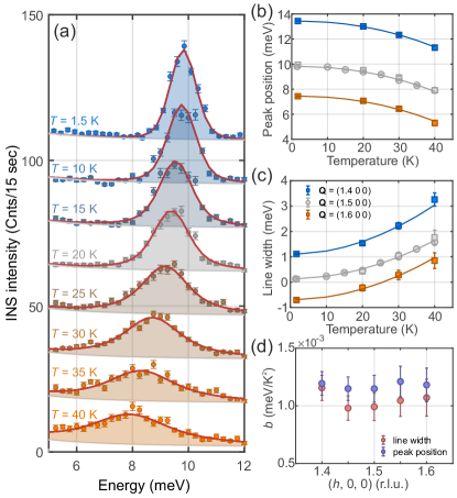
Figure 4: Thermal magnon renormalization at the M point. (a) Constant-$\mathbf{Q}$ cuts measured on EIGER at the M point, $\mathbf{Q}=(1.5~{}0~{}0)$. Spectra for the different temperatures are offset vertically by $+15$ units for clarity. Red lines show complete fits to the data composed of a Gaussian magnon contribution (shaded areas) and a temperature-independent background. (b,c) Dependence of the peak position (b) and line width (c) on temperature; solid lines show quadratic fits. Squares and circles correspond respectively to results obtained by fitting the PANTHER and EIGER datasets. (d) $\mathbf{Q}$-dependence of the quadratic fitting coefficients, $b$, through the M point.

Our first key result is the unambiguous demonstration of the data in Figs. 2(b) and 2(c) that the magnon bands have a Dirac dispersion through the K point, with no detectable splitting into acoustic and optical modes. It is important to contrast this conclusion with the recent INS study of Ref. Cai et al. (2021), which reported a large band splitting at the K point. In Sec. S2B of the SM SI we demonstrate that the reported splitting is not intrinsic to CrBr₃, but is rather an artifact arising from the large integration width applied in the analysis of the TOF dataset Do et al. (2022).

Thus we conclude that the low-temperature magnon dispersion in CrBr₃ has an ideal Dirac-cone nature with the Dirac point at $7.5\pm 0.1$ meV [Fig. 1(f)]. This is fully consistent with the inversion symmetry of the nearest-neighbor bond and the conventional $g$-factor values, both of which exclude significant DM effects. It is also consistent with all of the early INS results Samuelsen et al. (1971); Yelon and Silberglitt (1971), as we show in Sec. S2C of the SM SI . The Dirac cone in the 2D honeycomb FM was also used as a test case for the theoretical prediction Shivam et al. (2017) of a cosinusoidal intensity modulation arising from the isospin winding of near-nodal quasiparticles. This fingerprint has been observed recently in the honeycomb material CoTiO₃ Elliot et al. (2021) and in elemental Gd Scheie et al. (2022), and our results for the intensity distribution around the K point, shown in Fig. 1(h) and detailed in Sec. S2D of the SM SI , constitute its cleanest observation to date.

Next we use our low-temperature INS spectra to refine the spin Hamiltonian. Based on the lack of evidence for DM interactions in Fig. 2, but the very accurate measurement of a tiny spin gap at the $\Gamma$ point by ferromagnetic resonance (FMR) Dillon (1962); Alyoshin et al. (1997), we consider a Heisenberg model with single-ion anisotropy,

$$\mathcal{H}=\sum_{\langle i,j\rangle}J_{ij}\mathbf{S}_{i}\cdot\mathbf{S}_{j}+D\sum_{i}(S_{i}^{z})^{2}.$$ (1)

Here $\mathbf{S}_{i}$ is a $S=3/2$ spin operator, $J_{ij}$ are isotropic superexchange interactions between different Cr-ion pairs, and $D$ is the single-ion term. We determine the energies of the two magnon modes at 139 $\mathbf{Q}$ points by fitting the corresponding constant-$\mathbf{Q}$ cuts to two resolution-convolved Lorentz functions. We then use this dataset to fit the magnetic interactions in CrBr₃ by working within LSWT, as implemented in SpinW. We find the most accurate description of the observed spectra using three in-plane interactions and a very weak easy-axis anisotropy, as detailed in Sec. S3 of the SM SI . The optimal parameters we obtain for Eq. (1) are $J_{1}=-1.485(15)$, $J_{2}=-0.077(13)$, $J_{3}=0.068(12)$, and $D=-0.028(7)$ meV. Although we cannot detect the spin gap created by such a small anisotropy, we include the gap deduced from FMR in our fit. The excellent agreement between the observed and calculated INS spectra, both in dispersion and intensity distribution, is clear in Figs. 1(d-g) and 2(b-d).

Spin dynamics at finite temperature. Turning to thermal effects, Figs. 3(a) and 3(b) show two representative spectra collected respectively at $T=1.7$ and 30 K. Increasing $T$ clearly broadens the magnons and causes a downward energy shift, which decreases their band width. To quantify both effects, and their dependence on $\mathbf{Q}$, we used PANTHER to measure the spectral function at $T=20$, 30, and 40 K over several BZs. We made multiple constant-$\mathbf{Q}$ cuts covering four high-symmetry directions and fitted each peak with a Lorentzian broadening, convolved with the experimental resolution, to extract the positions and widths of the two magnon modes at each $T$ and $\mathbf{Q}$ point. Figure 3(c) summarizes the mode positions obtained at all four temperatures.

To visualize the effect of temperature on the magnon bands, we compute the normalized dispersion shift Yelon and Silberglitt (1971)

$$\Delta{\tilde{\varepsilon}}_{\mathbf{q}}(T)=\frac{\varepsilon_{\mathbf{q}}(0)-\varepsilon_{\mathbf{q}}(T)}{\varepsilon_{\mathbf{q}}(0)T^{2}},$$ (2)

where $\varepsilon_{\mathbf{q}}(0)$ denotes the dispersion measured at base temperature and $\varepsilon_{\mathbf{q}}(T)$ the corresponding finite-$T$ result. In the interacting SWT analysis of Ref. Pershoguba et al. (2018), the $T$-induced dispersion renormalization consists of a real Hartree term, $\Sigma_{1}(\mathbf{q})$, with a weak $\mathbf{q}$-dependence caused only by $J_{2}$, and a “sunset” term, $\Sigma_{2}(\mathbf{q})$. Because both are expected to show a $T^{2}$ form Bloch (1930); Pershoguba et al. (2018), we have included this factor in Eq. (2).

The symbols in Fig. 3(d) show the dispersion renormalization along the high-symmetry paths. The data for different temperatures collapse rather well to a single curve for both modes over the majority of the BZ, and we find that no change to the assumed $T^{2}$ form improves this collapse. To interpret this result, we have adapted the calculations of Ref. Pershoguba et al. (2018) to include the $J_{2}$ and $J_{3}$ terms, and present the details of this adaptation in Sec. S4 of the SM SI . We observe that $\Delta{\tilde{\varepsilon}}_{\mathbf{q}}(T)$ for the upper branch is described largely by the Hartree term alone, with the $\Sigma_{2}(\mathbf{q})$ contribution becoming sizeable only below the Dirac point.

Similarly, Fig. 3(e) demonstrates the analogous $T^{2}$ data reduction for the magnon line width. Again the experimental results for all temperatures collapse rather well, within their own uncertainties, to a single line. In this case, $J_{2}$ and $J_{3}$ have a qualitative role in removing line-width divergences that appear at the $\Gamma$ and M points due to the perfect nesting of the nearest-neighbor bands Pershoguba et al. (2018). However, even with these terms, the interacting SWT analysis predicts that both the line width and the band renormalization [Fig. 3(d)] should show multiple sharp peaks across the BZ, these “van Hove” features reflecting the underlying bare magnon bands Pershoguba et al. (2018), whereas our data do not support their presence.

A striking example is the difference between our data and the adapted SWT treatment around the M point, where the analysis predicts that both the energy and width of the 10 meV should show a sharp cusp, which is shifted slightly from M due to $J_{2}$ and $J_{3}$ [red lines in Figs. 3(d) and 3(e)]. To analyze the thermal renormalization in a fully quantitative manner, we used EIGER to measure the spectrum at the M point $\mathbf{Q}=(1.5~{}0~{}0)$ for multiple temperatures up to 40 K, as shown in Fig. 4(a). Figures 4(b) and 4(c) show respectively the dependences on $T$ of the magnon energy and line width extracted from both EIGER and PANTHER datasets. When fitted to the form $a+bT^{\alpha}$, the M-point data yield $\alpha_{\mathrm{Energy}}=2.25(15)$ and $\alpha_{\mathrm{Width}}=1.95(14)$, in good agreement with the expected value, $\alpha=2$. The same fitting at several $\mathbf{Q}$ points around ($1.5~{}0~{}0$) also yields quadratic forms for both quantities [Figs. 4(b,c)], while the prefactors $b$ that we extract show no appreciable changes with $\mathbf{Q}$ in Fig. 4(d), quite in contrast to interacting SWT.

Discussion. Our studies of thermal renormalization verify an ideal $T^{2}$ form, in fact above as well as below $T_{\mathrm{c}}$, as we have demonstrated in particular detail at the M point (Fig. 4). The origin of this behavior lies in the 2D nature of CrBr₃ and the quadratic dispersion at the band minimum, where thermally activated magnons cause the interaction effects responsible for band renormalization Bloch (1930). By a $T^{2}$ data reduction across the whole BZ, we find that the finite-$T$ magnon bands we have measured at high $\mathbf{q}$-resolution do not show features at the characteristic wave vectors found in a SWT analysis. This indicates that the $S=3/2$ honeycomb FM is subject to complex renormalization effects, arising from the combination of quantum and thermal fluctuations in the restricted phase space, whose accurate calculation calls for a more advanced (self-consistent and perhaps constrained) spin-wave treatment or for an unbiased numerical analysis by state-of-the-art quantum Monte Carlo Becker and Wessel (2018); Shao and Sandvik (2022) or matrix-product techniques Zauner-Stauber et al. (2018); Ponsioen et al. (2022).

To conclude, we have applied modern neutron spectrometry and data analysis to the layered honeycomb $S=3/2$ ferromagnet CrBr₃. At the band minimum we demonstrate quadratically dispersing magnons with a spin gap far below our base temperature. At the K point we demonstrate a near-perfect Dirac-cone dispersion with no discernible gapping, and we show that its topological consequences are reflected in the intensity winding. We obtain an accurate fit of the weak next-neighbor Heisenberg interactions, which remove the perfect honeycomb band nesting. At finite temperatures, the magnon renormalization obeys the expected $T^{2}$ form to very high accuracy. However, its dependence on the wave vector is not well reproduced at low order in spin-wave theory, indicating a need for more systematic calculations of mutual quantum and thermal renormalization effects in low-dimensional magnetism.

Acknowledgments. We acknowledge financial support from the Swiss National Science Foundation, the European Research Council grant Hyper Quantum Criticality (HyperQC), and the European Union Horizon 2020 research and innovation program under Marie Skłodowska-Curie Grant No. 884104. We thank the Institut Laue-Langevin and the Paul Scherrer Institute for the allocation of neutron beam-time.

Note added. During the completion of this manuscript we became aware that the data-analysis problem affecting the conclusions of Ref. Cai et al. (2021), which we analyze in Sec. S2B of the SM SI , has been demonstrated simultaneously for the sister compound CrCl₃ in Ref. Do et al. (2022).

Supplemental Material for “Thermal Evolution of Dirac Magnons

in the Honeycomb Ferromagnet CrBr₃”

S. E. Nikitin, B. Fåk, K. W. Krämer, T. Fennell, B. Normand, A. M. Läuchli, and Ch. Rüegg

S1 Sample preparation and characterization

S1.1 Crystal Growth

The crystal was prepared from CrBr₃ (Cerac, 3N), which first was sublimed for purification in a sealed silica ampoule at 700^∘ C under vacuum. For crystal growth, the purified material was sealed in a silica ampoule under vacuum and heated to 850^∘ C in a vertical tube furnace with a small temperature gradient. The crystal grew from the cold region over a period of three weeks. Afterwards, the ampoule was cooled to room temperature at a rate of 10 K per hour. All handling of the material was done under dry conditions in a glove box or in sealed sample containers.

S1.2 Mosaicity effects

The quality of the sample was characterized by neutron diffraction. We found that, in addition to the primary crystallite, it contained a structural twin whose in-plane axes were rotated by 30^∘ around the $c$ axis. From the ratio of the Bragg-peak intensities, we estimated that this twin constituted approximately 10% of the sample mass. To estimate the effects of such a twin on the INS spectra shown in Fig. 3(a) of the main text, which we reproduce in Fig. S1(a), we modelled the magnetic response of a composite system consisting of the twin and the main crystallite for each of the high-symmetry paths. As shown in Figs. S1(b) and S1(c), the twin produces two additional, faint magnon modes, whose traces can also be identified in our data [Fig. S1(a)]. Thus we took the twin contribution into account when extracting the positions and line widths of the measured magnon modes, by fitting it with a separate peak function at low temperatures, albeit with the relative positions, widths, and intensities of the twin-related peaks all fixed.

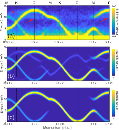
Figure S1: (a) Magnetic excitation spectra for the primary high-symmetry reciprocal-space directions in CrBr₃ taken from the PANTHER $E_{\mathrm{i}}=30$ meV dataset at $T=1.7$ K. This panel is reproduced from Fig. 3(a) of the main text and the red arrows indicate regions contaminated by the twin contribution. (b,c) Magnetic excitation spectrum calculated by LSWT with (b) and without (c) the twin contribution.

S2 INS experiment and data analysis

PANTHER is a direct-geometry TOF spectrometer at the ILL. The available beam time allowed us to collect data at $T=1.7$, 20, 30, and 40 K, each with two incident neutron energies, $E_{\mathrm{i}}=15$ and 30 meV, by rotating the crystal through $340^{\circ}$ in steps of 1^∘. Spectra were collected for 4 minutes at each angle with $E_{\mathrm{i}}=15$ meV and 3.5 minutes at 30 meV. The energy resolution, defined as the full width at half-maximum (FWHM) peak height at zero energy transfer were respectively 0.58 and 0.79 meV for $E_{\mathrm{i}}=15$ and $30$ meV. Reduction and analysis of the TOF data were performed using the software MANTID Arnold et al. (2014) and HORACE Ewings et al. (2016), and a symmetrization procedure was applied in order to improve the statistics. The result of this processing was a “four-dimensional” dataset of scattered intensities as a function of momentum transfer, $\mathbf{Q}$, and energy transfer, $\omega$, which we manipulate for different purposes in the remainder of this section.

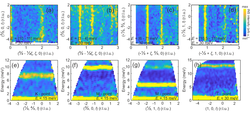
Figure S2: (a-d) Selected constant-energy cuts through the INS spectral function measured on PANTHER, which show essentially dispersionless behavior of the magnetic excitations in the out-of-plane direction, $l$. Data were integrated by $\pm 0.03$ r.l.u. in the orthogonal direction and over the energy ranges indicated; the intensity scales were optimized separately for each panel. (e-h) INS spectra taken at the high-symmetry K (e), M (f,g), and $\Gamma$ (h) points of the 2D BZ also show minimal dependence $l$; these intensity data were integrated by $\pm 0.03$ r.l.u. in the orthogonal directions and are shown on a common scale.

EIGER is a thermal-neutron TAS at the PSI. We used the fixed-$k_{\mathrm{f}}$ mode with $k_{\mathrm{f}}=2.662$ Å^-1, which yields an energy resolution (FWHM) of 0.63 meV at zero energy transfer, and collected data at eight different temperatures from 1.5 to 40 K. We set horizontal focusing on the analyzer and double focusing on the monochromator, also installing a graphite filter before the sample to reduce the contamination from second-order neutrons. We fitted the constant-$\mathbf{Q}$ cuts shown in Fig. 4 of the main text by using Eq. (S2), given in Sec. S3, in order to extract the center and width of the Lorentzian peak.

S2.1 Out-of-plane dispersion

Although the CrBr₃ sample was oriented in the $(h~{}k~{}0)$ scattering plane, the large vertical coverage of the position-sensitive detectors on PANTHER made it possible to collect some data from out-of-plane scattering. Figures S2(a-d) show constant-energy cuts through the 30 meV dataset taken at four different energies and transverse momentum transfers, in which the magnon branches exhibit no measurable dispersion as a function of $l$. Figures S2(e-h) show $\mathbf{Q}$-$E$ cuts along the $l$ direction taken at selected high-symmetry points, in which the magnon branches again appear almost completely flat. A very minor modulation at the upper band edge is consistent with fact that the ordering temperature, $T_{c}=32$ K, implies a weak interplane interaction, $J_{\perp}$, which the instrumental resolution prevents us from fitting accurately.

S2.2 Magnetic excitations near the Dirac point

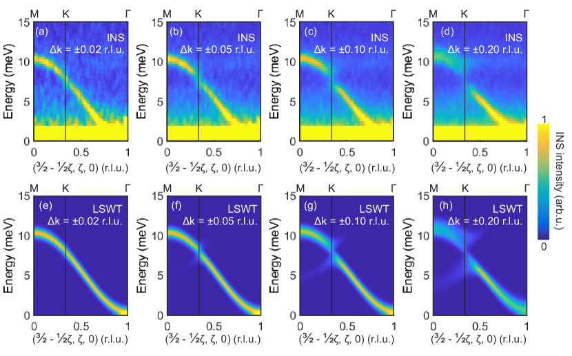
Figure S3: INS spectrum of CrBr₃ along the $(\frac{3}{2}-\frac{1}{2}\xi,\xi,0)$ direction. Panels (a-d) show results obtained by integrating the measured intensities over different widths ($\Delta k$) in the $k$ direction and panels (e-h) show the analogous results modelled within LSWT. It is clear that the spectrum is entirely continuous as $\Delta k$ is taken to zero, with only a dip in intensity at the K point arising due to the magnon density of states, whereas increasing $\Delta k$ causes the appearance of a spin gap at K. (i) Corresponding line widths extracted by using different values of $\Delta k$.

CrBr₃ has for 50 years been regarded as a prototypical honeycomb Heisenberg FM Samuelsen et al. (1971); Yelon and Silberglitt (1971), and for this reason was used as the test-case material in a recent analysis of the consequences of the Dirac cones in its magnon spectrum for its thermal and topological properties. Thus the recent work Cai and coauthors Cai et al. (2021) reporting a massive spin gap at the K point, of order 2 meV in a total band width of 13 meV, both contradicted previous results and would have profound consequences for the physical understanding of CrBr₃. Here we show that the conclusion of Ref. Cai et al. (2021) is contradicted by our data and we illustrate the most probable reason for this disagreement.

Like us, the authors of Ref. Cai et al. (2021) performed TOF INS experiments and in Figs. 1 and 3 of their manuscript present the spectra measured at their base temperature INS spectra by preparing $\mathbf{Q}$-$E$ cuts through the four-dimensional TOF datasets. In this type of analysis, it is necessary to choose an integration width in the two orthogonal directions in reciprocal space ($\mathbf{Q}$), and for this the authors used $\pm 0.2$ r.l.u. for the in-plane direction and $\pm 5$ out of plane. In this process, choosing a large window captures a higher intensity, allowing one to improve the statistics, but it can produce spurious features in the prepared cuts if the mode does disperse within the selected integration window. To illustrate this effect, in Figs. S3(a-d) we show multiple cuts from our PANTHER dataset ($E_{\mathrm{i}}=30$ meV, $T=1.7$ K) prepared by taking different integration widths, $\Delta{}k$, in the orthogonal in-plane direction. The spectrum we obtain with $\Delta{}k=\pm 0.2$ r.l.u. [Fig. S3(d)] gives the appearance of a robust splitting into separate acoustic and optical branches. However, if we decrease $\Delta{}k$ then this apparent gap also decreases, and with our data it is clear that there is no splitting for $\Delta{}k\leq 0.05$ r.l.u. [Figs. S3(a-b)].

To further support this observation, we have modelled the INS response of CrBr₃ by performing LSWT calculations within SpinW Toth and Lake (2015) using the spin Hamiltonian and Heisenberg interaction parameters given in and below Eq. (2) of the main text. In Figs. S3(e-h) we illustrate the results obtained by integrating the modelled intensity over the same ranges of orthogonal $\mathbf{q}$ as we did for the TOF data. It is clear that this modelling provides a perfect reproduction of the integrated INS data, supporting our conclusion that the splitting reported in Ref. Cai et al. (2021) is not a property of CrBr₃, but purely an extrinsic consequence of the data treatment.

The explanation of this effect is straighforward: the integration averages multiple intensity pixels in directions perpendicular to the cut. If there is little or no orthogonal dispersion across the integration window, the procedure is reliable. However, in a 2D honeycomb FM with a suspected Dirac cone at the K point, the only dispersionless direction is $l$; in $h$ and $k$, all the magnon intensity near the apex of the cone is concentrated in a small $\mathbf{Q}$ volume, and one should also note that this intensity is weak (the magnon density of states vanishes at a true Dirac point). A broad integration window risks missing the apical intensity and generates extra intensity at K at finite energies above and below the Dirac point, creating the appearance of broadened and separated magnon branches.

This integration-induced broadening also causes an apparent $\mathbf{Q}$-dependence of the magnon line width Xiao et al. (2022), an effect that can become substantial in parts of the BZ with strong dispersion. We modelled this broadening with SpinW and found that, for the in-plane integration widths we use ($\Delta h=\Delta k=\pm 0.03$ r.l.u.), it reaches 20% for the steepest parts of the magnon dispersion and rises rapidly if the integration width is increased. In preparing the results presented in Fig. 3 of the main text, we took both the instrumental resolution and this integration-induced broadening into account.

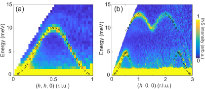
Figure S4: INS spectra prepared from the $E_{\mathrm{i}}=30$ meV PANTHER dataset at $T=1.7$ K for the high-symmetry directions $(h~{}0~{}0)$ (a) and $(h~{}h~{}0)$ (b). Points indicate experimental data taken from Fig. 6 of Ref. Samuelsen et al. (1971), which shows results obtained from measurements performed at a base temperature of 6 K.

S2.3 Comparison with previous INS studies

The magnon spectrum of CrBr₃ was measured in a series of INS experiments in the early 1970s Samuelsen et al. (1971); Yelon and Silberglitt (1971). Because a modern measurement of this spectrum Cai et al. (2021) contradicts these old results, but is also contradicted by our data (previous subsection), it is worthwhile to compare our results directly with the TAS data from Refs. Samuelsen et al. (1971); Yelon and Silberglitt (1971). In Fig. S4 we show on top of our PANTHER data the magnon center positions deduced by these authors at 6 K for the $(0~{}0~{}0)\rightarrow(1~{}1~{}0)$ and $(0~{}0~{}0)\rightarrow(3~{}0~{}0)$ paths in the BZ (which correspond to the $\Delta$ and $\Sigma$ directions in the notation of Ref. Samuelsen et al. (1971)). We conclude that the agreement is perfect within the resolutions of both measurements.

S2.4 Intensity winding of Dirac magnons

A recent theoretical analysis of Dirac and Weyl magnons predicted that the dynamical structure factor should exhibit a characteristic type of behavior in the vicinity of the special points Shivam et al. (2017). Using the honeycomb FM as their first example, these authors showed that the intensity should follow

$$I=I_{0}[1\pm\ \mathrm{cos}(\alpha-\alpha_{0})],$$ (S1)

on a circle taken in $\mathbf{Q}$ around the K point in the $l=0$ hexagonal plane; here $\alpha$ is the polar angle measured from $\alpha_{0}$ parallel to the $(h,0,0)$ direction [Fig. S5(a)] and the $\pm$ sign refers to the magnon bands above and below the Dirac point in energy. The origin of this behavior lies in the rotation of the isospin polarization of the magnon band, and examples have been observed very recently in experiments on CoTiO₃, a honeycomb magnet with bond-dependent interactions Elliot et al. (2021), and on elemental Gd, which has a hexagonal close-packed structure and RKKY-type magnetic interactions Scheie et al. (2022).

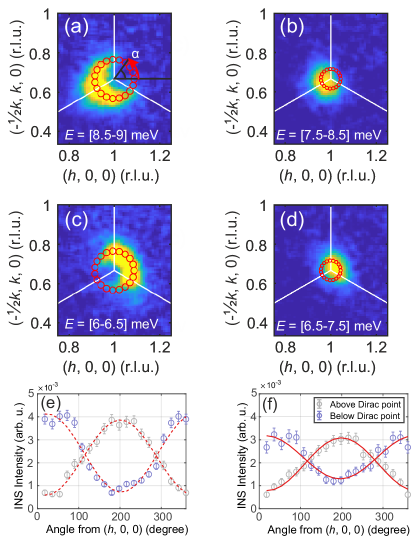
Figure S5: (a-d) Constant-energy cuts through the INS spectral function at energies above and below the Dirac-point energy of 7.5 meV. Data were taken from the $E_{\mathrm{i}}=30$ meV PANTHER measurements at $T=1.7$ K with integration performed over the momentum range $l=\pm 5$ and over the energy ranges shown. White lines show boundaries of the BZ and the axes in panel (a) show definition of $\alpha$ in Eq. (S1). (e) Intensity winding around the K point, shown as a function of angle on the path indicated in panels (a) and (c), which was chosen at $|\mathbf{q}|=0.08$ Å^-1 away from $\mathbf{q}=(2/3~{}2/3~{}0)$; this panel is also shown in Fig. 1(d) of the main text. (f) Intensity winding around the K point, shown as a function of angle on the path indicated in panels (b) and (d), which was chosen at $|\mathbf{q}|=0.04$ Å^-1 away from $\mathbf{q}=(2/3~{}2/3~{}0)$.

Figure 1(d) of the main text shows a near-ideal cosinusoidal intensity winding. These data were obtained from the constant-energy cuts shown in Figs. S5(a) and S5(c), which were taken respectively above and below the K point by integrating over energy windows of width 0.5 meV. In both cuts the INS intensity is concentrated around the K points and distributed over a semi-circular trajectory, but with peaks on the opposite sides of the K points for the upper and lower magnon bands. To quantify this effect and to compare it with theory [Eq. (S1)], we made azimuthal scans on the trajectory around the K point at $(2/3~{}2/3~{}0)$ that is indicated in both panels. It is clear from the curves in Fig. 1(d) of the main text, which are reproduced in Fig. S5(e), that the INS intensities on the bands above and below the Dirac point exhibit the anticipated cosine modulation with exactly opposing phases. In Figs. S5(b), S5(d), and S5(f) we show that this result is not particularly sensitive to the width of the integration window, at least in the regime of linear dispersion, although the trajectory should be redefined to match the shape of the Dirac cone. This perfect agreement with Eq. (S1) allows us to conclude that CrBr₃ provides an excellent realization of the isospin winding of nodal quasiparticles.

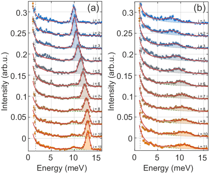
Figure S6: Constant-$\mathbf{Q}$ cuts taken from the $E_{\mathrm{i}}=30$ meV PANTHER datasets betewen $\mathbf{Q}=(1.5~{}0~{}0)$ ($i=1$) and $\mathbf{Q}=(1~{}0~{}0)$ ($i=11$) in steps of 0.05 r.l.u. Data were integrated over $\pm 0.03$ r.l.u. in the orthogonal in-plane directions and by $l=\pm 5$ r.l.u. out of plane, and are offset vertically for clarity. The spectra shown in panel (a) were collected at $T=1.7$ and in panel (b) at 40 K. Solid red lines show the total fit to the data, gray lines the background contribution, and filled areas the magnetic signal. We comment that some of the background curves in panels (a) include a weak inelastic peak arising from the twin contribution.

S3 Determination of the spin Hamiltonian

To extract the magnetic interaction parameters of CrBr₃ we used both PANTHER datasets measured at $T=1.7$ K, i.e. with $E_{\mathrm{i}}=15$ and 30 meV. We first quantified the positions of the magnon mode at 139 selected points in reciprocal space by fitting constant-$\mathbf{Q}$ cuts through the four-dimensional datasets to resolution-convolved Lorentz functions of the form

$$I(E)=a_{0}+a_{1}E^{-a_{2}}+\sum_{i=1}^{n}\mathrm{exp}\bigg{[}\frac{-E^{2}}{2W_{\mathrm{res}}^{2}}\bigg{]}\!*\!\frac{I_{i}\,\Gamma_{i}^{2}}{(E-\varepsilon_{i})^{2}+\Gamma_{i}^{2}},$$ (S2)

where $a_{0}$, $a_{1}$, and $a_{2}$ are empirical background parameters, $W_{\mathrm{res}}$ combines the (Gaussian) instrumental resolution and integration-induced broadening, $I_{i}$, $\varepsilon_{i}$, and $\Gamma_{i}$ are the intensity, position, and width of magnon peak $i$, $n$ is the number of magnon peaks, and the * denotes convolution. Examples of this fitting procedure are shown in Fig. S6(a), where intensity data for 11 $\mathbf{Q}$ points on the path $(1.5~{}0~{}0)\rightarrow(1~{}0~{}0)$ exhibit a single, strong, resolution-limited magnon mode in each case, whose center position disperses with $\mathbf{Q}$. For comparison, in Fig. S6(b) we also present an analysis of the INS spectra collected at our highest measurement temperature, $T=40$ K, where it is clear that the heights of the magnon peaks decrease considerably, they shift to lower energy, and they become significantly wider than the instrumental resolution, but remain clearly discernible. The positions and widths of the magnon modes extracted in this way were used in Fig. 3 of the main text. Returning to base temperature, we used multiple series of fits of the type shown in Fig. S6(a) to obtain a set of points $\{\varepsilon_{i}(\mathbf{q})\}$, which together characterize fully the experimental dispersion. These extracted mode positions are shown on top of the corresponding $\mathbf{Q}$-$E$ cuts in Figs. S7(a-g).

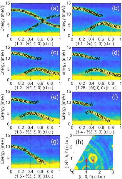
Figure S7: (a-g) INS spectra of CrBr₃ measured along multiple $\mathbf{Q}$ paths on PANTHER at $T=1.7$ K with $E_{\mathrm{i}}=30$ meV; the intensity scale is the same in all panels. The circles and error bars indicate respectively the mode positions and their statistical uncertainties obtained from fits to Eq. (S2). (h) Constant-energy cut in the $(h,k,0)$ scattering plane. Intensity data were obtained by integrating over the ranges $E=[2$–$3]$ meV and $l=\pm 5$ r.l.u. The red arrow shows the path used in panel (a), the purple arrow the path of panel (g), and panels (b-f) show parallel paths between the two arrows.

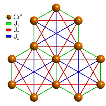
Figure S8: Representation of magnetic interactions in the honeycomb lattice formed by the Cr³⁺ ions (orange spheres) in a single layer of CrBr₃. Green, red, and blue lines indicate respectively the nearest- ($J_{1}$), second- ($J_{2}$), and third-neighbor ($J_{3}$) Heisenberg superexchange interactions.

Table S1: Magnetic interactions fitted to four spin models, which include different numbers of in-plane coupling parameters. $J_{m}$ and $D$ are respectively Heisenberg superexchange interactions and the single-ion anisotropy term, while $R_{W}$ quantifies the fit quality.

Model	$J_{1}$	$J_{2}$	$J_{3}$	$J_{4}$	$D$	$R_{W}$
$J_{1}$	$-1.44$	0	0	0	$-0.2$	9.59
$J_{1}$–$J_{2}$	$-1.46$	$-0.057$	0	0	$-0.02$	5.81
$J_{1}$–$J_{3}$	$-1.485$	$-0.077$	0.068	0	$-0.028$	2.05
$J_{1}$–$J_{4}$	$-1.494$	$-0.068$	0.067	0.0082	$-0.03$	1.96

To deduce the spin Hamiltonian of CrBr₃, we used the SpinW package Toth and Lake (2015) to calculate the low-temperature magnon dispersion and intensity of a model honeycomb FM, in order to compare the results with the set $\{\varepsilon_{i}(\mathbf{q})\}$ and with the corresponding measured intensities. As discussed in the main text, the models we consider have the form

$$\mathcal{H}=J_{1}\!\sum_{i,j}\mathbf{S}_{i}\cdot\mathbf{S}_{j}+J_{2}\!\sum_{\langle i,j\rangle}\!\mathbf{S}_{i}\cdot\mathbf{S}_{j}+J_{3}\!\!\sum_{\langle\langle i,j\rangle\rangle}\!\!\mathbf{S}_{i}\cdot\mathbf{S}_{j}+D\sum_{i}(S_{i}^{z})^{2},$$ (S3)

where the first, second, and third summations run over different nearest- and further-neighbor pairs of Cr³⁺ ions, as indicated in Fig. S8, and $D$ is the single-ion anisotropy term for the $S=3/2$ spins. In fact we tested four spin models, taking into account in-plane superexchange interactions, $J_{m}$, up to fourth neighbors, with the results summarized in Table S1. Starting with only a nearest-neighbor model, we found that introducing the second- and then the third-neighbor interactions each improves the quality of the fit quite considerably, with the optimal $J_{2}$ and $J_{3}$ values both being approximately 5% of $J_{1}$. By contrast, the introduction of $J_{4}$ has only a very minor effect on the fit quality and returns a value one order of magnitude smaller than $J_{2}$ and $J_{3}$. We therefore conclude that the minimal model for an accurate description of the spin dynamics in CrBr₃ is the $J_{1}$-$J_{2}$-$J_{3}$ model. We comment that, despite their small values, the effects of the $J_{2}$ and $J_{3}$ terms is in fact clearly visible in the magnon dispersions shown in Figs. 2 and 3 of the main text, because they act to lift the Dirac point from 6.5 meV, in a $J_{1}$ model that has two branches with energies 0 and 13 meV at the $\Gamma$ point, to 7.5 meV in CrBr₃, and a similar 1 meV shift is found at the M point.

We comment that the resolution of our INS experiments did not allow us to determine precisely a possible spin gap at the $\Gamma$ point, where the signal is dominated by an elastic peak. However, a spin gap, $\Delta(\Gamma)$, can be measured very accurately by the method of ferromagnetic resonance (FMR), and for CrBr₃ one finds $\Delta(\Gamma)=0.08$ meV at $T=2$ K Dillon (1962); Alyoshin et al. (1997). With this information we performed our fits in two different ways: (i) considering only our INS data and (ii) taking into account the FMR value of $\Delta(\Gamma)$. Our fits (i) yielded a value $\Delta(\Gamma)=0.2$ meV, which on the scale of the overall magnon band width is not a large discrepancy. All of the Heisenberg interactions remained the same within their error bars for both fitting procedures, with only the value of $D$ changing. Thus we fitted $D$ to the FMR value of $\Delta(\Gamma)$ and used the INS data without constraint to obtain the most accurate superexchange parameters for the spin Hamiltonian of CrBr₃.

S4 Adapted interacting SWT calculation of magnon self-energies

To compare with our measurements of the thermal renormalization of the magnon dispersion and width, we followed Ref. Pershoguba et al. (2018) to perform calculations of the magnon self-energy for the $J_{1}$-$J_{2}$-$J_{3}$ model of Sec. S3. These authors computed the lowest-order spin-wave interaction terms, which are the Hartree contribution, $\Sigma_{1}(\mathbf{q})$, and the “sunset” contribution, $\Sigma_{2}(\mathbf{q})$, for the situation with two magnon branches in the folded BZ that arises for the simplest non-Bravais lattices. In both contributions, one of the incoming magnons is thermally excited around the band minimum ($\mathbf{q}=0$) and can be neglected in the interaction process, but causes the finite-temperature renormalization whose $T^{2}$ form is a straightforward consequence of the dimensionality factors summarized in the main text Bloch (1930); Pershoguba et al. (2018).

Considering first the Hartree part, $\Sigma_{1}(\mathbf{q})$ is a real quantity that in the $J_{1}$ model is constant across the entire BZ as a consequence of the special property of these two bands. In the $J_{1}$-$J_{2}$-$J_{3}$ case, $\Sigma_{1}(\mathbf{q})$ regains a weak $\mathbf{q}$-dependence due to the $J_{2}$ term. The $\mathbf{q}$-dependence of $\Sigma_{2}(\mathbf{q})$ arises from an integral over one internal magnon momentum and takes the form

$${\rm Re}\,\Sigma_{2}(\mathbf{q})=\alpha T^{2}\!\!\int\!\!d^{2}p\,\frac{|v_{\mathbf{q};\mathbf{p}}|^{2}\,(\varepsilon_{\mathbf{q}}-\varepsilon_{\mathbf{p}}-\varepsilon_{\mathbf{q}-\mathbf{p}})}{(\varepsilon_{\mathbf{q}}-\varepsilon_{\mathbf{p}}-\varepsilon_{\mathbf{q}-\mathbf{p}})^{2}+\eta^{2}}$$ (S4)

for the real part and

$${\rm Im}\,\Sigma_{2}(\mathbf{q})=\alpha\pi T^{2}\!\!\int\!\!d^{2}p\,|v_{\mathbf{q};\mathbf{p}}|^{2}\,\delta(\varepsilon_{\mathbf{q}}-\varepsilon_{\mathbf{p}}-\varepsilon_{\mathbf{q}-\mathbf{p}})$$ (S5)

for the imaginary part. In these expressions, $\varepsilon_{\mathbf{q}}$ is the magnon dispersion relation, $\eta$ is a broadening function, and $|v_{\mathbf{q};\mathbf{p}}|$ denotes the matrix elements of the magnon-magnon interaction processes. The authors of Ref. Pershoguba et al. (2018) made a detailed analysis of these matrix elements, but in the calculation of the real part encountered a historical problem Dyson (1956a, b) arising in the long-wavelength limit and as a result reverted to some ad hoc matrix-element expressions.

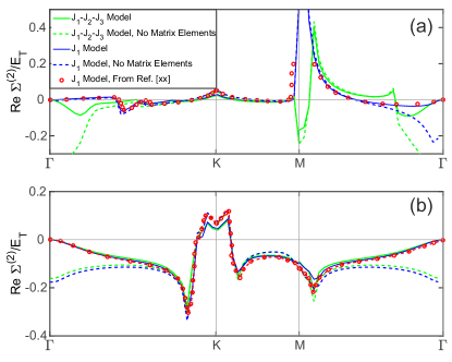
Figure S9: Interacting SWT calculation of the real part of the magnon self-energy for the magnon branches above (a) and below (b) the Dirac-point energy. This band renormalization is computed for the nearest-neighbor ($J_{1}$) honeycomb model with and without the matrix elements proposed in Ref. Pershoguba et al. (2018), and is compared with the analogous results obtained for the $J_{1}$-$J_{2}$-$J_{3}$ magnon bands of Sec. S3. The unit of energy is $E_{T}=T^{2}/J_{1}S^{3}$.

In computing the real and imaginary self-energies for the full $J_{1}$-$J_{2}$-$J_{3}$ magnon dispersion, we have followed Ref. Pershoguba et al. (2018) by adopting their ad hoc matrix elements in Eq. (S4) and by scaling their final result in Eq. (S5). In this process we benefitted from their observation that the matrix elements are well behaved functions of wave vector that do not introduce any singular behavior and we performed calculations with $J_{2}=J_{3}=0$ that reproduced theirs, as shown in Figs. S9 and S10. This allowed us to obtain the final band renormalizations directly in Fig. S9, where the structure of the calculation requires attributing the self-energies to the upper and lower magnon branches, rather than to modes 1 and 2, and to obtain the final line widths in Fig. S10 by scaling to our results with the experimental values of $J_{2}$ and $J_{3}$. We also benefitted from the analysis of prefactors ($\alpha$ in Eq. (S4) and (S5)) provided in Ref. Pershoguba et al. (2018) such that our calculated magnitudes of the magnon shift and line width have the same “parameter-free” status as theirs. In relating the calculated ${\rm Im}\,\Sigma(\mathbf{q})$ to the measured line widths in Fig. 3(e) of the main text, we assumed that they correspond to the HWHM of the Lorentzian fitting function [Eq. (S2)].

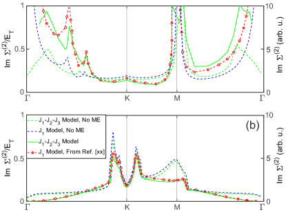
Figure S10: Interacting SWT calculation of the imaginary part of the magnon self-energy for the magnon branches above (a) and below (b) the Dirac-point energy. The $\delta$-function part of the self-energy is computed for both the nearest-neighbor ($J_{1}$) and the $J_{1}$-$J_{2}$-$J_{3}$ magnon bands without including matrix elements (denoted ME), and then the magnon line width for the $J_{1}$-$J_{2}$-$J_{3}$ case is obtained by scaling the result of Ref. Pershoguba et al. (2018) for the $J_{1}$ case with matrix elements. Calculations without matrix elements (dotted lines) are shown on the same arbitrary scale (right $y$ axis), while the results with matrix elements are shown in units of $E_{\mathrm{T}}$ (left $y$ axis).

By inspecting the $\mathbf{q}$-dependence of the thermal renormalization and line width, we find that the interacting SWT calculations for the $J_{1}$-$J_{2}$-$J_{3}$ bands continue to predict multiple characteristic peaks. With the exception of divergences in the line width at $\Gamma$ and M, which are consequences of perfect nesting in the $J_{1}$ model, all of the van Hove cusps found in Ref. Pershoguba et al. (2018) are only slightly moved or blunted. By contrast, our reduced data in Figs. 3(d) and 3(e) of the main text show a total lack of characteristic features as a function of $\mathbf{q}$. Beyond the flat response around the M point shown in Fig. 4 of the main text, we also do not find evidence, within the uncertainties of our data, for the peak near the K point highlighted in Ref. Pershoguba et al. (2018) (we comment that the appearance of this feature in the results of Ref. Yelon and Silberglitt (1971) is in fact based on a single data point). We remark that the largest values of the reduced band shift and line width visible in Figs. 3(d) and 3(e) of the main text appear where the magnon energy in the denominator of Eq. (2) of the main text is small, and this is the reason for the large uncertainties on all of these data points.

Thus one must conclude that the van Hove features are artifacts of the low level of approximation in the interacting spin-wave calculation. In particular, the energetic renormalization of the band, ${\rm Re}\,\Sigma(\mathbf{q})$, can be expected to have a significant effect on the nesting contributions to the interaction terms, and it would be necessary to include this self-consistently. It is also possible that the $S=3/2$ nature of the quantum spins should be included in a constrained spin-wave treatment, and that it may have significant consequences for nesting effects even at the $1/S$ level. Beyond a more sophisticated spin-wave treatment, in the main text we also draw attention to the rapid advances taking place in the numerical calculation of spectral functions for quantum magnetic models within the framework of stochastic analytic continuation quantum Monte Carlo methods and separately within the framework of tensor-network techniques.

References

- Novoselov et al. (2004) K. S. Novoselov, A. K. Geim, S. V. Morozov, D.-e. Jiang, Y. Zhang, S. V. Dubonos, I. V. Grigorieva, and A. A. Firsov, Science 306, 666 (2004).
- Novoselov et al. (2005) K. S. Novoselov, A. K. Geim, S. V. Morozov, D. Jiang, M. I. Katsnelson, I. Grigorieva, S. Dubonos, and A. Firsov, Nature 438, 197 (2005).
- Geim (2009) A. K. Geim, Science 324, 1530 (2009).
- Pershoguba et al. (2018) S. S. Pershoguba, S. Banerjee, J. Lashley, J. Park, H. Ågren, G. Aeppli, and A. V. Balatsky, Phys. Rev. X 8, 011010 (2018).
- Li et al. (2017) K. Li, C. Li, J. Hu, Y. Li, and C. Fang, Phys. Rev. Lett. 119, 247202 (2017).
- McClarty (2022) P. McClarty, Annu. Rev. Condens. Matter Phys. 13, 171 (2022).
- Mook et al. (2021) A. Mook, K. Plekhanov, J. Klinovaja, and D. Loss, Phys. Rev. X 11, 021061 (2021).
- Yao et al. (2018) W. Yao, C. Li, L. Wang, S. Xue, Y. Dan, K. Iida, K. Kamazawa, K. Li, C. Fang, and Y. Li, Nat. Phys. 14, 1011 (2018).
- Chen et al. (2018) L. Chen, J.-H. Chung, B. Gao, T. Chen, M. B. Stone, A. I. Kolesnikov, Q. Huang, and P. Dai, Phys. Rev. X 8, 041028 (2018).
- Yuan et al. (2020) B. Yuan, I. Khait, G.-J. Shu, F. C. Chou, M. B. Stone, J. P. Clancy, A. Paramekanti, and Y.-J. Kim, Phys. Rev. X 10, 011062 (2020).
- Elliot et al. (2021) M. Elliot, P. A. McClarty, D. Prabhakaran, R. D. Johnson, H. C. Walker, P. Manuel, and R. Coldea, Nat. Commun. 12, 3936 (2021).
- Cai et al. (2021) Z. Cai, S. Bao, Z.-L. Gu, Y.-P. Gao, Z. Ma, Y. Shangguan, W. Si, Z.-Y. Dong, W. Wang, Y. Wu, D. Lin, J. Wang, K. Ran, S. Li, D. Adroja, X. Xi, S.-L. Yu, J.-X. Li, and J. Wen, Phys. Rev. B 104, L020402 (2021).
- Scheie et al. (2022) A. Scheie, P. Laurell, P. A. CcClarty, G. E. Granroth, M. B. Stone, R. Moessner, and S. E. Nagler, Phys. Rev. Lett. 128, 097201 (2022).
- Chumak et al. (2015) A. V. Chumak, V. I. Vasyuchka, A. A. Serga, and B. Hillebrands, Nat. Phys. 11, 453 (2015).
- Wang et al. (2018) X. S. Wang, H. W. Zhang, and X. R. Wang, Phys. Rev. Appl. 9, 024029 (2018).
- Pirro et al. (2021) P. Pirro, V. I. Vasyuchka, A. A. Serga, and B. Hillebrands, Nat. Rev. Mater. 6, 1114 (2021).
- Chen et al. (2021) L. Chen, M. B. Stone, A. I. Kolesnikov, B. Winn, W. Shon, P. Dai, and J.-H. Chung, 2D Mater. 9, 015006 (2021).
- Morosin and Narath (1964) B. Morosin and A. Narath, J. Chem. Phys. 40, 1958 (1964).
- Samuelsen et al. (1971) E. J. Samuelsen, R. Silberglitt, G. Shirane, and J. P. Remeika, Phys. Rev. B 3, 157 (1971).
- McGuire et al. (2015) M. A. McGuire, H. Dixit, V. R. Cooper, and B. A. Sales, Chem. Mater. 27, 612 (2015).
- Wang et al. (2011) H. Wang, V. Eyert, and U. Schwingenschlögl, J. Phys.: Condens. Matter 23, 116003 (2011).
- Do et al. (2022) S.-H. Do, J. A. M. Paddison, G. Sala, T. J. Williams, K. Kaneko, K. Kuwahara, A. F. May, J. Yan, M. A. McGuire, M. D. Stone, M. D. Lumsden, and A. D. Christianson, arXiv:2204.03720 (2022).
- Yelon and Silberglitt (1971) W. B. Yelon and R. Silberglitt, Phys. Rev. B 4, 2280 (1971).
- (24) See the Supplemental Materials at http://www.xxx.yyy, which contains Refs. Xiao et al. (2022); Dyson (1956a, b), for a full exposition of our data reduction and fitting, of the bin-width error that can appear as a gap at the Dirac point, of the intensity winding property at this point, of the comparison with literature results, and of the adapted SWT calculations we perform to obtain the first-order magnon self-energy in the -- model.
- (25) https://www.ill.eu/users/instruments/instrument-list/ panther.
- Nikitin et al. (2021) S. Nikitin, B. Fåk, K. W. Krämer, and C. Rüegg, (2021), doi:10.5291/ILL-DATA.DIR-236.
- Stuhr et al. (2017) U. Stuhr, B. Roessli, S. Gvasaliya, H. M. Rønnow, U. Filges, D. Graf, A. Bollhalder, D. Hohl, R. Bürge, M. Schild, L. Holitzner, C. Kaegi, P. Keller, and T. Mühlebach, Nucl. Instrum. Meth. A 853, 16 (2017).
- Arnold et al. (2014) O. Arnold, J. C. Bilheux, J. M. Borreguero, A. Buts, S. I. Campbell, L. Chapon, M. Doucet, N. Draper, R. F. Leal, M. A. Gigg, V. E. Lynch, A. Markvardsen, D. J. Mikkelson, R. L. Mikkelson, R. Miller, K. Palmen, P. Parker, G. Passos, T. G. Perring, P. F. Peterson, S. Ren, M. A. Reuter, A. T. Savici, J. W. Taylor, R. J. Taylor, R. Tolchenov, W. Zhou, and J. Zikovsky, Nucl. Instrum. Meth. A 764, 156 (2014).
- Ewings et al. (2016) R. A. Ewings, A. Buts, M. D. Le, J. van Duijn, I. Bustinduy, and T. G. Perring, Nucl. Instrum. Meth. A 834, 3132 (2016).
- Toth and Lake (2015) S. Toth and B. Lake, J. Phys.: Condens. Matter 27, 166002 (2015).
- Alyoshin et al. (1997) V. Alyoshin, V. Berezin, and V. Tulin, Phys. Rev. B 56, 719 (1997).
- Shivam et al. (2017) S. Shivam, R. Coldea, R. Moessner, and P. McClarty, arXiv:1712.08535 (2017).
- Dillon (1962) J. Dillon, in Proceedings of the Seventh Conference on Magnetism and Magnetic Materials (Springer, 1962) pp. 1191–1192.
- Bloch (1930) F. Bloch, Z. Phys. 61, 206 (1930).
- Becker and Wessel (2018) J. Becker and S. Wessel, Phys. Rev. Lett. 121, 077202 (2018).
- Shao and Sandvik (2022) H. Shao and A. W. Sandvik, arXiv:2202.09870 (2022).
- Zauner-Stauber et al. (2018) V. Zauner-Stauber, L. Vanderstraeten, J. Haegeman, I. P. McCulloch, and F. Verstraete, Phys. Rev. B 97, 235155 (2018).
- Ponsioen et al. (2022) B. Ponsioen, F. F. Assaad, and P. Corboz, SciPost Phys. 12, 006 (2022).
- Xiao et al. (2022) E. Xiao, H. Ma, M. S. Bryan, L. Fu, J. M. Mann, B. Winn, D. L. Abernathy, R. P. Hermann, A. R. Khanolkar, C. A. Dennett, D. H. Hurley, M. E. Manley, and C. A. Marianetti, arXiv:2202.11041 (2022).
- Dyson (1956a) F. J. Dyson, Phys. Rev. 102, 1217 (1956a).
- Dyson (1956b) F. J. Dyson, Phys. Rev. 102, 1230 (1956b).