Casimir Self-Entropy of Nanoparticles with Classical Polarizabilities: Electromagnetic Field Fluctuations

Abstract

Not only are Casimir interaction entropies not guaranteed to be positive, but also, more strikingly, Casimir self-entropies of bodies can be negative. Here, we attempt to interpret the physical origin and meaning of these negative self-entropies by investigating the Casimir self-entropy of a neutral spherical nanoparticle. After extracting the polarizabilities of such a particle by examining the asymptotic behavior of the scattering Green’s function, we compute the corresponding free energy and entropy. Two models for the nanoparticle, namely a spherical plasma $\delta$-function shell and a homogeneous dielectric/diamagnetic ball, are considered at low temperature, because that is all that can be revealed from a nanoparticle perspective. The second model includes a contribution to the entropy from the bulk free energy, referring to the situation where the medium inside or outside the ball fills all space, which must be subtracted on physical grounds in order to maintain consistency with van der Waals interactions, corresponding to the self-entropy of each bulk. (The van der Waals calculation is described in Appendix A.) The entropies so calculated agree with known results in the low-temperature limit, appropriate for a small particle, and are negative. But we suggest that the negative self-entropy is simply an interaction entropy, the difference between the total entropy and the blackbody entropy of the two bulks, outside or inside of the nanosphere. The vacuum entropy is always positive and overwhelms the interaction entropy. Thus the interaction entropy can be negative, without contradicting the principles of statistical thermodynamics. Given the intrinsic electrical properties of the nanoparticle, the self-entropy arises from its interaction with the thermal vacuum permeating all space. Because the entropy of blackbody radiation by itself plays an important role, it is also discussed, including dispersive effects, in detail.

I Introduction

When an electromagnetic quantum field coexists in thermal equilibrium with bodies or boundaries, the entropy of the system will be altered by their presence, which may lead to nontrivial phenomena implying novel physics and applications. This additional entropy, known as Casimir entropy, was recognized as a physical quantity in the debate on how to model a metal within a finite-temperature environment, when evaluating the Casimir force between metal plates. Initially, there were claims that the Drude model resulted in Casimir entropies inconsistent with the third law of thermodynamics Bezerra et al. (2004); Klimchitskaya and Korikov (2015); Korikov (2016); Klimchitskaya and Mostepanenko (2017), but it has been shown that this does not occur for real materials Brevik et al. (2006); Milton et al. (2012). Experimentally, results favoring both the plasma model Decca et al. (2005); Banishev et al. (2013); Bimonte et al. (2016); Liu et al. (2019); Klimchitskaya and Mostepanenko (2021), which does not include dissipation, and the Drude model Sushkov et al. (2011); Garcia-Sanchez et al. (2012), which does, have been reported. This inconsistency with the physically motivated Drude model has not yet been resolved, but the subject of Casimir entropy by itself has drawn much attention.

Casimir interaction entropy, caused by the interactions between two or more bodies via the fluctuating quantum electromagnetic field, has been intensively investigated for many years due to its fascinating properties, such as its negativity Bezerra et al. (2002a, b); Canaguier-Durand et al. (2010); Rodriguez-Lopez (2011); Ingold et al. (2015); Milton et al. (2015); Umrath et al. (2015); Milton et al. (2017a). Less investigated, however, is the Casimir self-entropy, resulting from the self-interaction of a single body, which provides us with further intriguing possibilities and puzzles to be understood. We will concentrate on a new approach to this problem in this paper.

In Ref. Li et al. (2016), we evaluated the Casimir self-entropy of a plasma $\delta$-function plate (PDP), with the aim of justifying the widely accepted hypothesis that the negative Casimir interaction entropy would always be compensated by corresponding positive self-entropies. We obtained analytic formulas for the transverse electric (TE) and transvese magnetic (TM) contributions to the PDP self-entropy. They both satisfy the third law of thermodynamics, in that the entropy vanishes as the temperature goes to zero, and indeed the total self-entropy is positive, although the TE contribution is always negative. But, in the strong-coupling limit, which is the perfectly conducting (PC) case, the total self-entropy approaches zero, which eliminates the possibility that it can cancel the negative interaction entropy between a PC sphere and a PC plate. In Refs. Li et al. (2016); Milton et al. (2017a), we showed, however, that the Casimir self-entropy of a PC sphere precisely cancels the most negative part of the interaction entropy between a sphere and a plate. Then we generalized our study of Casimir self-entropy to the model of a plasma $\delta$-function spherical shell (PDS). Various regularization schemes were employed to evaluate the TE and TM self-entropies of a PDS in limiting cases in Ref. Milton et al. (2017b). It was especially surprising to find that, when the coupling was weak enough, both the TE and TM self-entropies are negative—See Eq. (1). Bordag and Kirsten examined the same plasma-shell model Bordag (2018); Bordag and Kirsten (2018), but obtained somewhat different results; their results were technically equivalent to those in Ref. Milton et al. (2017b), differing only in certain subtractions. For more detailed comparisons, please refer to Ref. Milton et al. (2019). Most recently, we utilized a numerical method, based on the Abel-Plana formula, to elucidate general behaviors of PDS self-entropies Li et al. (2021), which confirms the results in Ref. Milton et al. (2017b) and clearly demonstrates the existence of negative self-entropy. So, in contrast to the naive hypothesis, Casimir self-entropy can be quite nontrivial, and its negativity needs to be better understood.

According to Ref. Milton et al. (2017b), the leading terms of TE and TM PDS self-entropies are negative and of the first order in the coupling $\lambda_{0}$, specifically,

$$S^{\text{TE}}_{(1)}=-\lambda_{0}\bigg{(}\frac{t}{6}+\frac{1}{2t}-\frac{1}{2}\coth t\bigg{)},\quad S^{\text{TM}}_{(1)}=-\lambda_{0}\bigg{(}\frac{t}{18}-\frac{1}{2t}+\frac{1}{2}\coth t\bigg{)},$$ (1)

in which $t=2\pi aT$, $a$ is the radius of the spherical shell, and $T$ is the temperature. The terms linear in $\lambda_{0}$ might be supposed to originate from the self-interaction of each point in the material, in analogy with $\lambda\phi^{4}$ theory, although here the coupling refers to the entire surface of the sphere. It is conventional wisdom that this kind of self-interaction should be subtracted off, as a “tadpole” term; doing so here, however, would destroy the passage to the perfectly-conducting limit. The appearance of negative Casimir self-entropy and its linear dependence on the coupling in PDS imply the necessity of investigating the influence of the self-interaction more delicately, so that the meaning of negative Casimir self-entropy and the remaining divergences encountered in spherical systems, or even of their consequences in reality, could be clarified.

For a homogeneous dielectric ball (DB), it is known that the bulk contributions must be subtracted Milton et al. (2020), but even with this so-called bulk subtraction, the zero-temperature calculations are plagued with ambiguous divergences Milton and Brevik (2018), except for special cases where the speed of light is the same inside and outside the spherical boundary Milton et al. (1978); Brevik and Kolbenstvedt (1982). Recently, Avni and Leonhardt Avni and Leonhardt (2018) claimed that their subtracted physical Casimir stresses on a dielectric ball yields an energy, depending linearly on the susceptibility in the weak-coupling limit, and thus violating the interpretation in terms of van der Waals forces. Some of us have argued that their conclusions are erroneous Milton et al. (2020). This matter is still being disputed Efrat and Leonhardt (2021). Here, we will extend the calculations of Ref. Milton et al. (2020) to finite temperature.

We focus on a system composed of a nanoparticle that interacts with a thermal electromagnetic background (blackbody radiation) and that is characterized by macroscopic polarizability parameters, inferred from the large-distance behavior of the Green’s functions describing electromagnetic scattering. As it is viewed from far away, the particle appears as a point. The entropy can be calculated directly in terms of these polarizabilities in a standard way. In this manner, we hope to shed light on the self-interaction influences alone. In Sec. II, we extract the polarizabilites, expressed in terms of the reflection coefficients in the scattering Green’s function. We consider two models for the nanoparticle, the PDS model mentioned above, and the homogeneous nondispersive dielectric/diamagnetic ball. We compute the corresponding entropies in Sec. III. The contributions depending linearly on the polarizability are clearly identified. In Sec. IV, we show the necessity, in the DB case, for subtracting the bulk contributions to achieve consistency with known results, and with the interpretation in terms of the van der Waals interactions between the constituents of the nanoparticle. This bulk subtraction corresponds to removal of the entropy change due to the replacement of a volume of vacuum by a corresponding volume of dielectric material. In Appendix B we show that negative self-entropies correspond to what we call interaction entropies, which can be of any sign, and are overwhelmed by the positive blackbody entropy. Because the interaction with the blackbody radiation field plays an important role, in Sec. V, we examine the entropy of the background, with and without permittivity/permeability, including dispersion described by the plasma model. The blackbody entropy is well-known in vacuum, but less so in a homogeneous medium. Especially interesting is the behavior of the entropy in the presence of a dispersive background. Conclusions are presented in Sec. VI. Appendix A provides evidence that the bulk subtraction for the dielectric sphere is required for all temperatures. Appendix A also supplies a derivation of the low-temperature free energy of a dilute dielectric sphere, based on summation of van der Waals interactions, applying a variation of a method used two decades ago by Barton Barton (2001a). The results for the entropy agree with those found in the main text. The results are also confirmed by the analysis presented in Appendix B. Appendix C shows that our results for the low-temperature self-entropy for a dielectric/diamagnetic sphere follow immediately by extending the zero-temperature self-energy derived long ago Milton (1980); Milton and Ng (1997); Milton (2001) to finite temperature. Natural units $\hbar=\varepsilon_{0}=\mu_{0}=c=k_{B}=1$ are used throughout. That is, we use rationalized Heaviside-Lorentz units, where the relation between Gaussian and Heaviside-Lorentz polarizabilities is given by $\alpha^{\rm HL}=4\pi\alpha^{\rm G}$.

II Extraction of Classical Polarizabilities

In this paper, we work with macroscopic electromagnetic theory, written in terms of Euclidean frequencies. Firstly, to see that bulk materials and point-like particles could be dealt with on the same footing, here we show how a small spherical particle of material behaves as a microscopically large but macroscopically small object, which we will refer to as a “nanoparticle” for short.

II.1 Classical Polarizabilities

The Green’s dyadic, $\bm{\Gamma}$, for a given Euclidean frequency, $\zeta$, satisfies

$$\left[-\bm{\varepsilon}(\zeta,\mathbf{r})-\frac{\bm{\nabla}\times\bm{\mu}^{-1}(\zeta,\mathbf{r})\cdot\bm{\nabla}\times\bm{1}}{\zeta^{2}}\right]\cdot\bm{\Gamma}(\zeta;\mathbf{r},\mathbf{r}^{\prime})=\bm{1}\delta(\mathbf{r}-\mathbf{r}^{\prime}).$$ (2)

Without losing much generality, suppose the permittivity and permeability of the system are both isotropic and inhomogeneous only in the radial direction. For points outside the object, the Green’s dyadic, $\bm{\Gamma}(\zeta;\mathbf{r},\mathbf{r}^{\prime})$, is written simply as Milton and Ng (1997)

$$\bm{\Gamma}(\zeta;\mathbf{r},\mathbf{r}^{\prime})=\sum_{l=1}^{\infty}\sum_{m=-l}^{l}\left[-\bm{\nabla}\times g_{\zeta,l}^{H}(r,r^{\prime})\mathbf{X}^{m}_{l}(\Omega)\mathbf{X}^{m*}_{l}(\Omega^{\prime})\times\overleftarrow{\bm{\nabla}}^{\prime}-\zeta^{2}g_{\zeta,l}^{E}(r,r^{\prime})\mathbf{X}^{m}_{l}(\Omega)\mathbf{X}^{m*}_{l}(\Omega^{\prime})\right],$$ (3a)

in which the vector spherical harmonics are defined as

$$\mathbf{X}^{m}_{l}(\Omega)=\frac{\mathbf{L}Y^{m}_{l}(\Omega)}{\sqrt{l(l+1)}},\quad\mathbf{L}=\mathbf{r}\times\frac{1}{i}\bm{\nabla}.$$ (3b)

The reduced Green’s functions $$g^{E}_{\zeta,l},\ g^{H}_{\zeta,l}$$ satisfy the equations

$$\left[-r\frac{d}{dr}\frac{1}{(\mu,\varepsilon)}\frac{d}{dr}r+\frac{l(l+1)}{(\mu,\varepsilon)}+(\varepsilon,\mu)\zeta^{2}r^{2}\right]g^{(E,H)}_{\zeta,l}(r,r^{\prime})=\delta(r-r^{\prime}).$$ (3c)

The solutions for the TE and TM Green’s functions in vacuum outside a spherical particle of radius $a$ are ($\kappa=|\zeta|$)

$$g_{\zeta,l}^{E,H}(r,r^{\prime})=\frac{1}{\kappa rr^{\prime}}\left[s_{l}(\kappa r_{<})e_{l}(\kappa r_{>})+R_{l}^{E,H}(\kappa a)e_{l}(\kappa r)e_{l}(\kappa r^{\prime})\right],\quad r,r^{\prime}>a,$$ (4)

in terms of the appropriate reflection coefficients (Mie coefficients) for the particle, where $s_{l}$ and $e_{l}$ are modified Riccati-Bessel functions. Explicit examples will be given in the following. We refer to the terms in the Green’s function proportional to the reflection coefficients as the scattering parts.

Imagine that source and field points are far from the particle, $r,r^{\prime}\gg a$. Then, the reflection coefficients are to be evaluated for small values of $\kappa a$. In general, this means that only the $l=1$ term in the scattering Green’s dyadic needs to be retained, since $R_{1}\gg R_{l\neq 1}$ in this limit. This follows from the behavior for small arguments of the modified Riccati-Bessel functions,

$$e_{l}(x)\sim\frac{1}{x^{l}}\frac{2^{l}\Gamma(l+1/2)}{\sqrt{\pi}},\quad s_{l}(x)\sim x^{l+1}\frac{\sqrt{\pi}}{2^{l+1}\Gamma(l+3/2)},\quad x\ll 1.$$ (5)

On the other hand, suppose the permittivity and permeability of the particle are written in terms of electric and magnetic polarizabilities, $\bm{\alpha}$ and $\bm{\beta}$, as $\bm{\varepsilon}(\zeta,\mathbf{r})=\bm{1}+\bm{\alpha}(\zeta)\delta(\mathbf{r})$ and $\bm{\mu}^{-1}(\zeta,\mathbf{r})=\bm{1}-\bm{\beta}(\zeta)\delta(\mathbf{r})$. Then, based on a generalization of the method given in Ref. Schwinger et al. (1998), pp. 277–8, we can identify the polarizabilities of the particle, by analyzing the above Green’s dyadic, (3). As shown in Fig. 1, the free Green’s dyadic, $\bm{\Gamma}_{0}(\zeta;\mathbf{r,r^{\prime}})$, is represented by the line going directly from $\mathbf{r^{\prime}}$ to $\mathbf{r}$. The scattering part has a propagator going from $\mathbf{r^{\prime}}$ to the nanoparticle, $\bm{\Gamma}_{0}(\zeta;\mathbf{r^{\prime\prime},r^{\prime}})$, and a second one going from the nanoparticle to the observer at $\mathbf{r}$, $\bm{\Gamma}_{0}(\zeta;\mathbf{r,r^{\prime\prime}})$. The interaction is effected via the polarizability of the nanoparticle, located at $\mathbf{r^{\prime\prime}=0}$. The sum of these two contributions gives the total Green’s dyadic. Because the particle is small, the single scattering approximation is sufficient.

Figure 1: Sketch of the scattering process used to extract the polarizability of the nanoparticle.

The scattering part of the TE part of the Green’s dyadic can be written in terms of $\bm{\Gamma}_{0}$ and the polarizabilities of the particle as

$$\bm{\Gamma}_{\rm Sc}^{E}(\zeta;\mathbf{r},\mathbf{r}^{\prime})-\bm{\Gamma}_{0}(\zeta;\mathbf{r},\mathbf{r}^{\prime\prime})\times\overleftarrow{\bm{\nabla}}^{\prime\prime}\cdot\frac{\bm{\beta}(\zeta)}{\zeta^{2}}\cdot\bm{\nabla}^{\prime\prime}\times\bm{\Gamma}(\zeta;\mathbf{r}^{\prime\prime},\mathbf{r}^{\prime})+\bm{\Gamma}_{0}(\zeta;\mathbf{r},\mathbf{r}^{\prime\prime})\cdot\bm{\alpha}(\zeta)\cdot\bm{\Gamma}(\zeta;\mathbf{r}^{\prime\prime},\mathbf{r}^{\prime}),\quad\mathbf{r}^{\prime\prime}\rightarrow\bm{0},$$ (6)

where the magnetic polarizability, $\bm{\beta}$, couples to the magnetic field, given by Faraday’s law, $\bm{\nabla}\times\mathbf{E}=-\zeta\mathbf{B}$, while the electric polarizability, $\bm{\alpha}$, couples to the electric field. ($\bm{\Gamma}$ represents a vacuum expectation value of the product of electric fields.) In Eq. (6) we have assumed that the particle has no extent. Schematically, the effective polarizabilities $\bm{\alpha}$ and $\bm{\beta}$ satisfy the following relation

$$\bm{\Gamma}_{\rm Sc}^{E}-\bm{\Gamma}_{0}\left[\times\overleftarrow{\bm{\nabla}}\frac{\bm{\beta}}{\zeta^{2}}\bm{\nabla}\times-\bm{\alpha}\right]\bm{\Gamma}_{0},$$ (7)

where we have noted that, because the polarizabilities are small, we may replace $\bm{\Gamma}$ by $\bm{\Gamma}_{0}$ on the right.

Now we use the orthonormality properties of the vector spherical harmonics,

$$\int d\Omega\,\mathbf{X}^{*}_{lm}(\Omega)\cdot\mathbf{X}_{l^{\prime}m^{\prime}}(\Omega) = \delta_{ll^{\prime}}\delta_{mm^{\prime}},$$ (8a)

$$\int d\Omega[f(r^{\prime})\mathbf{X}_{lm}(\Omega)]^{*}\cdot[\bm{\nabla}\times g(r)\mathbf{X}_{lm}(\Omega)] = 0,$$ (8b)

$$\int d\Omega\,[\bm{\nabla}^{\prime}\times f(r^{\prime})\mathbf{X}_{lm}(\Omega)]^{*}\cdot[\bm{\nabla}\times g(r)\mathbf{X}_{lm}(\Omega)] = \frac{1}{rr^{\prime}}\left[\frac{d}{dr^{\prime}}(r^{\prime}f(r^{\prime})^{*})\frac{d}{dr}(rg(r))+l(l+1)f(r^{\prime})^{*}g(r)\right]\delta_{ll^{\prime}}\delta_{mm^{\prime}}.\quad$$ (8c)

Then, because $l=1$ dominates for a small particle, we see that only the magnetic polarizability term contributes to the TE scattering Green’s dyadic, which we take to be isotropic:

$$\beta^{E}=\frac{3}{2}\frac{4\pi}{\kappa^{3}}R_{1}^{E},\quad\alpha^{E}=0.$$ (9)

Similar arguments apply to the TM contribution. The TM part of $\bm{\Gamma}_{\rm Sc}$ is

$$\bm{\Gamma}^{H}_{\rm Sc}(\zeta;\mathbf{r,r^{\prime}})\bigg{|}_{l=1}=-R^{H}_{1}\bm{\nabla}\times\frac{e_{1}(\kappa r)e_{1}(\kappa r^{\prime})}{\kappa rr^{\prime}}\sum_{m}\mathbf{X}_{1m}(\Omega)\mathbf{X}^{*}_{1m}(\Omega^{\prime})\times\overleftarrow{\bm{\nabla}^{\prime}}.$$ (10)

The decomposition in terms of scattering with the electric and magnetic polarizabilites of the particle is

$$\bm{\Gamma}^{H}_{\rm Sc}(\zeta;\mathbf{r,r^{\prime}})\sim\sum_{m,m^{\prime}}\bigg{\{}\bm{\nabla}\times\frac{e_{1}(\kappa r)s_{1}(\kappa r^{\prime\prime})}{\kappa rr^{\prime\prime}}\mathbf{X}_{1m}(\Omega)\mathbf{X}^{*}_{1m}(\Omega^{\prime\prime})\times\overleftarrow{\bm{\nabla}}^{\prime\prime}\cdot\alpha^{H}\cdot\bm{\nabla}^{\prime\prime}\times\frac{s_{1}(\kappa r^{\prime\prime})e_{1}(\kappa r^{\prime})}{\kappa r^{\prime\prime}r^{\prime}}\mathbf{X}_{1m^{\prime}}(\Omega^{\prime\prime})\mathbf{X}^{*}_{1m^{\prime}}(\Omega^{\prime})\times\overleftarrow{\bm{\nabla}}^{\prime}$$

$$\mbox{}-\frac{1}{\kappa^{2}}\bm{\nabla}\times\frac{e_{1}(\kappa r)s_{1}(\kappa r^{\prime\prime})}{\kappa rr^{\prime\prime}}\mathbf{X}_{1m}(\Omega)\mathbf{X}^{*}_{1m}(\Omega^{\prime\prime})\times\overleftarrow{\bm{\nabla}}^{\prime\prime}\times\overleftarrow{\bm{\nabla}}^{\prime\prime}\cdot\beta^{H}\cdot\bm{\nabla}^{\prime\prime}\times\bm{\nabla}^{\prime\prime}\times\frac{s_{1}(\kappa r^{\prime\prime})e_{1}(\kappa r^{\prime})}{\kappa r^{\prime\prime}r^{\prime}}\mathbf{X}_{1m^{\prime}}(\Omega^{\prime\prime})\mathbf{X}^{*}_{1m^{\prime}}(\Omega^{\prime})\times\overleftarrow{\bm{\nabla}}^{\prime}\bigg{\}}.$$

Each double curl can be replaced by $-\kappa^{2}$, and then it is evident that the second term above vanishes in the $r^{\prime\prime}\to 0$ limit. Employing the averaging over solid angles as above for the first term, and using the identity (8c), we see immediately that the electric polarizability arises from the TM scattering Green’s dyadic:

$$\alpha^{H}=\frac{3}{2}\frac{4\pi}{\kappa^{3}}R_{1}^{H},\quad\beta^{H}=0.$$ (12)

II.2 Examples

To be more specific, we now turn to particular models.

II.2.1 $\delta$-Function Spherical Shell

To get a first indication of how the microscopic structure of a nanoparticle influences its macroscopic behavior, let us consider an example previously investigated in Ref. Milton et al. (2017b), namely the $\delta$-function spherical shell of radius $a$. Suppose the permittivity and permeability of the system are $\bm{\varepsilon}=\bm{1}+\lambda_{e}a(\bm{1}-\hat{\mathbf{r}}\hat{\mathbf{r}})\delta(r-a)$ and $\bm{\mu}=\bm{1}+\lambda_{m}a(\bm{1}-\hat{\mathbf{r}}\hat{\mathbf{r}})\delta(r-a)$, respectively. According to the arguments in Ref. Parashar et al. (2017), we have required that the polarizabilities normal to the shell surface are zero. The TE reflection coefficient is given by Parashar et al. (2017); Milton (2011)

$$R_{l}^{E}=\frac{\lambda_{m}a\kappa s_{l}^{\prime 2}(\kappa a)-\lambda_{e}a\kappa s_{l}^{2}(\kappa a)}{1-\lambda_{m}a\kappa e^{\prime}_{l}(\kappa a)s^{\prime}_{l}(\kappa a)+\lambda_{e}a\kappa e_{l}(\kappa a)s_{l}(\kappa a)+\frac{\lambda_{e}\lambda_{m}a^{2}\kappa^{2}}{4}},$$ (13a)

and the corresponding TM coefficient, $$R_{l}^{H} \lambda_{e}\leftrightarrow\lambda_{m}$$, can be obtained with the substitution as

$$R_{l}^{H}=\frac{\lambda_{e}a\kappa s_{l}^{\prime 2}(\kappa a)-\lambda_{m}a\kappa s_{l}^{2}(\kappa a)}{1-\lambda_{e}a\kappa e^{\prime}_{l}(\kappa a)s^{\prime}_{l}(\kappa a)+\lambda_{m}a\kappa e_{l}(\kappa a)s_{l}(\kappa a)+\frac{\lambda_{e}\lambda_{m}a^{2}\kappa^{2}}{4}}.$$ (13b)

For simplicity, consider the case in which $\lambda_{e}\neq 0,\lambda_{m}=0$, so that $R^{E}$ and $R^{H}$ reduce to

$$R_{l}^{E}=-\frac{\lambda_{e}a\kappa s_{l}^{2}(\kappa a)}{1+\lambda_{e}a\kappa e_{l}(\kappa a)s_{l}(\kappa a)},\ R_{l}^{H}=\frac{\lambda_{e}a\kappa s_{l}^{\prime 2}(\kappa a)}{1-\lambda_{e}a\kappa e^{\prime}_{l}(\kappa a)s^{\prime}_{l}(\kappa a)}.$$ (14)

This means that in the point approximation, $a\rightarrow 0$, where the small argument approximations (5) are applicable, the effective polarizabilities of the nanoparticle, dominated by $l=1$, are expressed as

$$\beta=\beta^{E}=-\frac{\lambda_{e}(\kappa a)^{2}/6}{1+\lambda_{e}(\kappa a)^{2}/3}4\pi a^{3},\quad\alpha=\alpha^{H}=\frac{2\lambda_{e}/3}{1+2\lambda_{e}/3}4\pi a^{3}.$$ (15)

Particularly, as in the model used in Refs. Li et al. (2016); Bordag and Kirsten (2018), consider dispersion as given by a plasma model, i.e., $\lambda_{e}=\lambda_{0}/(\kappa a)^{2}$. Then, from Eqs. (15), the nonzero polarizabilities for the $\delta$-function sphere are

$$\beta^{E}=-\frac{\lambda_{0}/6}{1+\lambda_{0}/3}4\pi a^{3},\quad\alpha^{H}=\frac{\frac{2}{3}\frac{\lambda_{0}}{(\kappa a)^{2}}}{1+\frac{2}{3}\frac{\lambda_{0}}{(\kappa a)^{2}}}4\pi a^{3}.$$ (16)

As expected, $\alpha^{H}\to 4\pi a^{3}$ in the strong-coupling limit, while in that limit $\beta^{E}\to-\frac{1}{2}4\pi a^{3}$. The electric polarizability possesses dispersion in general.

If we keep both $\lambda_{e},\lambda_{m}$ nonzero, then, in the point approximation, $\kappa a\to 0$, $R_{1}^{E}$ and $R_{1}^{H}$ are approximated as

$$R_{1}^{E}\approx\frac{\frac{4}{9}\lambda_{m}(\kappa a)^{3}-\frac{1}{9}\lambda_{e}(\kappa a)^{5}}{1+\frac{2}{3}\lambda_{m}+(\frac{1}{3}\lambda_{e}+\frac{\lambda_{e}\lambda_{m}}{4})(\kappa a)^{2}},\quad R_{1}^{H}\approx\frac{\frac{4}{9}\lambda_{e}(\kappa a)^{3}-\frac{1}{9}\lambda_{m}(\kappa a)^{5}}{1+\frac{2}{3}\lambda_{e}+(\frac{1}{3}\lambda_{m}+\frac{\lambda_{e}\lambda_{m}}{4})(\kappa a)^{2}},$$ (17)

which lead us to the magnetic and electric polarizabilities

$$\beta^{E}=\frac{\frac{2}{3}\lambda_{m}-\frac{1}{6}\lambda_{e}(\kappa a)^{2}}{1+\frac{2}{3}\lambda_{m}+(\frac{1}{3}\lambda_{e}+\frac{\lambda_{e}\lambda_{m}}{4})(\kappa a)^{2}}4\pi a^{3},\quad\alpha^{H}=\frac{\frac{2}{3}\lambda_{e}-\frac{1}{6}\lambda_{m}(\kappa a)^{2}}{1+\frac{2}{3}\lambda_{e}+(\frac{1}{3}\lambda_{m}+\frac{\lambda_{e}\lambda_{m}}{4})(\kappa a)^{2}}4\pi a^{3}.$$ (18)

We will not pursue the effects of $\lambda_{m}$ further here.

II.2.2 Dielectric Ball

As a second and more realistic example, we study a homogeneous dielectric ball of radius $a$ with nondispersive permittivity $\varepsilon$ and permeability $\mu$, immersed in vacuum. The reflection coefficients are Milton and Ng (1997)

$$R_{l}^{E}=-\frac{s_{l}(\widetilde{\kappa}a)s_{l}^{\prime}(\kappa a)-\sqrt{\frac{\varepsilon}{\mu}}s_{l}(\kappa a)s_{l}^{\prime}(\widetilde{\kappa}a)}{s_{l}(\widetilde{\kappa}a)e_{l}^{\prime}(\kappa a)-\sqrt{\frac{\varepsilon}{\mu}}e_{l}(\kappa a)s_{l}^{\prime}(\widetilde{\kappa}a)},\quad R^{H}_{l}=-\frac{\sqrt{\frac{\varepsilon}{\mu}}s_{l}(\widetilde{\kappa}a)s_{l}^{\prime}(\kappa a)-s_{l}(\kappa a)s_{l}^{\prime}(\widetilde{\kappa}a)}{\sqrt{\frac{\varepsilon}{\mu}}s_{l}(\widetilde{\kappa}a)e_{l}^{\prime}(\kappa a)-e_{l}(\kappa a)s_{l}^{\prime}(\widetilde{\kappa}a)}.$$ (19)

Here $\kappa=|\zeta|$, while $\widetilde{\kappa}=\sqrt{\varepsilon\mu}\kappa$. We proceed as above, and require the small $a$ limit, where

$$R_{1}^{E}=\frac{2}{3}\frac{\mu-1}{\mu+2}(\kappa a)^{3}+O\big{[}(\kappa a)^{5}\big{]},\quad R_{1}^{H}\sim\frac{2}{3}\frac{\varepsilon-1}{\varepsilon+2}(\kappa a)^{3}+O\big{[}(\kappa a)^{5}\big{]},\quad\kappa a\ll 1,$$ (20)

Only the terms of order $(\kappa a)^{3}$ will survive, so it follows that the TE contribution to the magnetic polarizabilities is nonzero, if the ball is permeable,

$$\alpha^{E}=0,\quad\beta^{E}=\frac{\mu-1}{\mu+2}4\pi a^{3},$$ (21)

while the TM part yields an electric polarizability depending on the permittivity,

$$\alpha^{H}=\frac{\varepsilon-1}{\varepsilon+2}4\pi a^{3},\quad\beta^{H}=0.$$ (22)

This electric polarizability is just that found in electrostatics Schwinger et al. (1998). Again, in the perfectly conducting limit, the polarizabilities tend to their expected values,

$$\alpha^{H}\to 4\pi a^{3},\quad\beta^{E}\to-\frac{1}{2}4\pi a^{3},\quad\varepsilon\to\infty,\,\mu\to 0.$$ (23)

For both the $\delta$-function spherical shell and dielectric ball examples, the point-approximated polarizabilities are proportional to the volume of the nanoparticle, which is consistent with the small-polarizability assumption adopted in Eq. (6). Furthermore, although the constituents of the dielectric ball interact, as explicitly demonstrated in Appendix A, the Clausius-Mossotti equation, which in our approximation incorporates those interactions, means that the polarizabilities are linearly related to their corresponding microscopic counterparts; that is, the polarizability of the nanoparticle is simply the sum of the polarizabilities of its microscopic constituents. This is discussed in detail in Appendix B.

III Particle Description of Casimir Self-Entropy

Now we arrive at the main topic of this paper, namely the Casimir self-entropy, which is just the additional entropy of the thermal field induced by a single object in it, when the effects of the thermal blackbody field have been properly removed. As has been stated in Sec. I, we saw interesting contributions from self-interaction, which we would like to investigate with the illustrative particle models here.

Because of the different frequency dependencies, the contributions to the free energy can have quite different behavior for small polarizabilites. We compute the free energy from the sum over Matsubara frequencies ($\zeta_{m}=2\pi Tm$)

$$F=\frac{T}{2}\sum_{m=-\infty}^{\infty}e^{i\zeta_{m}\tau}\operatorname{Tr}\ln(\bm{1}-\bm{\Gamma}_{0}\mathbf{V})\approx-\frac{T}{2}\int(d\mathbf{r^{\prime}})\sum_{m=-\infty}^{\infty}e^{i\zeta_{m}\tau}\operatorname{tr}\bm{\Gamma}_{0}(\zeta_{m};\mathbf{r,r^{\prime}})\mathbf{V}(\zeta_{m},\mathbf{r^{\prime}})\bigg{|}_{\mathbf{r=r^{\prime}}+\bm{\rho}},$$ (24)

which has been regulated by point-splitting in time, $\tau$, and in space, $\bm{\rho}$. Here, we treat the potential of the isotropic polarizable point particle as

$$\mathbf{V}_{e}(\zeta_{m},\mathbf{r^{\prime}})=\bm{1}\alpha(\zeta_{m})\delta(\mathbf{r^{\prime}}),\quad\mathbf{V}_{m}(\zeta_{m},\mathbf{r^{\prime}})=\bm{1}\beta(\zeta_{m})\delta(\mathbf{r^{\prime}}).$$ (25)

The reason for retaining only the first order in the potential is that the particle is small, not that the coupling, $\lambda$, $\varepsilon-1$, or $\mu-1$, is weak. The trace of the Green’s dyadic is

$$\operatorname{tr}\bm{\Gamma}_{0}(\zeta;\bm{\rho},\bm{0})\big{|}_{\bm{\rho}\to\bm{0}}=\operatorname{tr}(\bm{\nabla\nabla}-\bm{1}\nabla^{2})\frac{e^{-|\zeta|r}}{4\pi r}\bigg{|}_{r=\rho\to 0}=-2\zeta^{2}\frac{e^{-|\zeta|\rho}}{4\pi\rho},\quad\rho=|\bm{\rho}|\to 0,$$ (26)

which uses the scalar Green’s function equation

$$\left(-\nabla^{2}+\zeta^{2}\right)\frac{e^{-|\zeta|r}}{4\pi r}=\delta(\mathbf{r}).$$ (27)

It is important that the spherical symmetry be respected by the regulator, in this case the distance between the two points, $\rho$.

In addition to dispersion, anisotropy of the particle could also play a significant role. Here, however, we cannot contradict the spherical symmetry requirement, but it might be expected that the particle could have a polarizability of the form $\bm{\alpha}=\alpha(\bm{1}-\mathbf{\hat{r}^{\prime\prime}\hat{r}^{\prime\prime}})$. However, it is easily seen that the radial-radial component of the Green’s dyadic is zero, so this is without effect.

III.1 $\delta$-Function Spherical Shell

We first consider the $\delta$-function spherical shell model above. Using the polarizability $\beta^{E}$ in Eq. (16), if we only employ spatial point-splitting, that is, set $\tau=0$, we find, as $\rho\to 0$

$$F^{E}=-\frac{1}{6}\frac{\lambda_{0}}{1+\lambda_{0}/3}a^{3}\left(\frac{2}{\pi\rho^{4}}-\frac{2\pi^{3}T^{4}}{15}\right),\quad aT\ll 1,$$ (28)

where the restriction on $T$ emerges from the point-particle limit. In contrast, $\alpha^{H}$ has nontrivial frequency dependence. For the weak-coupling TM contribution, there is an additional $1/\zeta^{2}$ factor, so the behavior is given by

$$F^{H}=\frac{2}{3}\frac{\lambda_{0}}{a^{2}}a^{3}\left(\frac{1}{\pi\rho^{2}}+\frac{\pi}{3}T^{2}\right),\quad\lambda_{0}\ll 1,\,\,aT\ll 1.$$ (29)

For strong coupling, the TM contribution is the same form as the TE, except for the replacement of $\beta^{E}=-\frac{1}{2}4\pi a^{3}$ by $\alpha^{H}=-2\beta^{E}=4\pi a^{3}$. The divergent terms for both the TE and TM contributions are independent of temperature, so the weak-coupling, low-temperature entropies are with $t=2\pi aT$

$$S^{E}=-\lambda_{0}\frac{t^{3}}{90},\quad S^{H}=-\frac{2}{9}\lambda_{0}t,$$ (30)

which are exactly the results found in Ref. Milton et al. (2017b). The strong coupling limits are given by

$$S_{\infty}^{H}=-2S_{\infty}^{E}=\frac{t^{3}}{15},$$ (31)

which are consistent with the well-known perfectly-conducting sphere results for low temperature Balian and Duplantier (1978). Note that in weak coupling, the total self-entropy is negative, while it is positive in strong coupling.

III.2 Dielectric/Diamagnetic Ball

We now turn to the homogeneous dielectric/diamagnetic ball. Following the same procedure, we find for the free energies, assuming the absence of dispersion [see Eq. (22) and Eq. (21)],

$$F^{H,E}=\frac{1}{4\pi}\left(\begin{array}[]{c}\alpha^{H}\\ \beta^{E}\end{array}\right)\left(\frac{2}{\pi\rho^{4}}-\frac{2\pi^{3}T^{4}}{15}\right).$$ (34)

If we use the point-splitting in time rather than in space,that is, keep $\tau\neq 0$, but set $\rho=0$, we encounter

$$\sum_{m=-\infty}^{\infty}e^{i\zeta_{m}\tau}\operatorname{tr}\bm{\Gamma}_{0}(\zeta_{m})=-\frac{1}{2\pi}\sum_{m=-\infty}^{\infty}e^{i\zeta_{m}\tau}\zeta_{m}^{2}\left(\frac{1}{\rho}-|\zeta_{m}|\right),$$ (35)

where we have expanded Eq. (26) for small $\rho$. The first term here is proportional to a second derivative of a $\delta$-function in $\tau$ [see Eq. (77)], so is to be omitted, while the second is

$$\frac{i}{2\pi}\left(\frac{\partial}{\partial\tau}\right)^{3}\left[\frac{1}{1-e^{i2\pi T\tau}}-\frac{1}{1-e^{-i2\pi T\tau}}\right].$$ (36)

Carrying out the differentiation and expanding now in $\tau$, we obtain

$$F^{H,E}=\frac{1}{4\pi}\left(\begin{array}[]{c}\alpha^{H}\\ \beta^{E}\end{array}\right)\left(-\frac{6}{\pi\tau^{4}}-\frac{2\pi^{3}T^{4}}{15}\right),$$ (39)

where the $-3$ ratio in the coefficients of the divergence is expected on general grounds Milton et al. (2013). [See, for example, Eq. (57).] Both Eqs. (34) and (39) have the same finite part, which yields the total self-entropy ($t=2\pi aT$)

$$S=S^{H}+S^{E}=\left(\frac{\varepsilon-1}{\varepsilon+2}+\frac{\mu-1}{\mu+2}\right)\frac{t^{3}}{15}.$$ (40)

This has the correct strong-coupling (perfectly-conducting) $\varepsilon\to\infty$, $\mu\to 0$ limit in Eq. (31). Comparing Eq. (30) and Eq. (40), we see how different models of the nanoparticle can lead to entirely disparate behaviors of the self-entropy. In particular, this entropy is positive for $\varepsilon>1$, $\mu>1$, although it could be of either sign if one of these inequalities is violated.

For dilute constituents of the dielectric/diamagnetic ball, we evidently see terms depending linearly on the susceptibilities $\varepsilon-1$ and $\mu-1$ in Eq. (40). This is extraordinary and seems, at first sight, inexplicable, considering well-established understandings. We showed Milton et al. (2020), at zero temperature, that the free energy should begin, in the dilute limit for a pure dielectric ball, as $(\varepsilon-1)^{2}$, which is understood as originating from the pairwise summation of van der Waals interactions. The free energy was also calculated many years ago by Nesterenko, Lambiase, and Scarpetta  Nesterenko et al. (2001), and by Barton Barton (2001a, b)

$$F=\frac{23}{1536}\frac{(\varepsilon-1)^{2}}{\pi a}+\frac{7}{270}(\varepsilon-1)^{2}\pi^{3}a^{3}T^{4}.$$ (41)

The first term, corresponding to zero temperature, was first calculated by Milton and Ng (by summing van der Waals interactions) Milton and Ng (1998) and by Brevik, Marashevsky, and Milton (by expanding the Casimir energy) Brevik et al. (1999). The authors of Ref. Nesterenko et al. (2001) seem not to remark that the corresponding entropy is negative,

$$S=-\frac{7}{540}(\varepsilon-1)^{2}t^{3},\quad|\varepsilon-1|\ll 1.$$ (42)

So, the initial linear behavior in $\varepsilon-1$ seen in Eq. (40) is not present. Although there might be some differences between Casimir entropies of a nanoparticle and a bulk dielectric ball, it is still puzzling to see this discrepancy, which will be dealt with in the following section.

IV Bulk free energy

Hitherto, we have been considering a point particle. The conundrum mentioned at the end of the preceding section arises when we recognize that an extended object appears as a point far away from the object. The formula obtained for the additional free energy resulting from the insertion of the particle into the thermal bath therefore includes everything. However, when one looks at the ball in the near field and considers it as an extended object, one must recognize that an additional part of the free energy comes from the replacement of a point particle (of zero volume) by a medium of finite volume—in effect, this finite volume of the medium “displaces” what was previously considered the same volume of vacuum in the far field, point particle, perspective. This part of the additional free energy must therefore be subtracted in order to be left with the true additional free energy due to the interaction, and this subtraction is the finite temperature bulk subtraction. The need for this subtraction here is simply because the initial setup regarded the particle as a point, and the finite extension of the particle itself contributes a change to the free energy of that volume, which is in a sense extraneous to what is being sought here, and so must be subtracted.

This way of extracting a meaningful self-free energy for the dielectric ball is what is conventionally done, in order to obtain consistency with van der Waals interactions. That is, we subtract the contribution that would be obtained if either the interior or the exterior medium filled all of space. This was discussed recently in detail in Ref. Milton et al. (2020), but only at zero temperature. We can follow the method articulated in Appendix A of that reference. The most unambiguous way to proceed is to start with the pressure on the sphere, which is the discontinuity, across the surface, of the radial-radial stress tensor component,

$$p^{(0)}(\varepsilon,\mu;\varepsilon^{\prime},\mu^{\prime};a)=T^{(0)}_{rr}(\varepsilon,\mu;a_{-})-T^{(0)}_{rr}(\varepsilon^{\prime},\mu^{\prime};a_{+}),$$ (43)

where the two stress tensors refer to a homogeneous medium, either $\varepsilon$, $\mu$, or $\varepsilon^{\prime}$, $\mu^{\prime}$ filling all space, and $a_{\pm}$ means the corresponding stress tensor is evaluated just outside or just inside the spherical boundary of the dielectric/diamagnetic sphere. (In our case, $\varepsilon^{\prime}$ and $\mu^{\prime}$ are both set equal to unity.) Here, in each region, using the Matsubara frequency decomposition at finite temperature $T$, the use of which is equivalent to that of the fluctuation-dissipation theorem)

$$T_{rr}^{(0)}(\varepsilon,\mu,a_{-})=\frac{1}{2a^{4}}aT\sum_{m=-\infty}^{\infty}e^{i\zeta_{m}\tau}\sum_{l=1}^{\infty}\frac{2l+1}{4\pi}f_{l}(x_{m}),$$ (44)

with $x_{m}=2\pi|m|aT\sqrt{\varepsilon\mu}$, with the summand being

$$f_{l}(x)=2x[s_{l}^{\prime}(x)e_{l}^{\prime}(x)-s_{l}^{\prime\prime}(x)e_{l}(x)]=2\frac{\partial}{\partial r}\left(\frac{\partial}{\partial s}-\frac{\partial}{\partial r}\right)\frac{s_{l}(rx)e_{l}(sx)}{x}\bigg{|}_{s>r>1,s\to 1}.$$ (45)

Now using the addition theorem, with $s>r$,

$$\sum_{l=0}^{\infty}(2l+1)s_{l}(rx)e_{l}(sx)=\frac{xrs}{s-r}e^{-x(s-r)},$$ (46)

we see that the bulk stress tensor is

$$T_{rr}^{(0)}(\varepsilon,\mu;a_{-}) = \frac{T}{4\pi a^{3}}\sum_{m=-\infty}^{\infty}e^{i\zeta_{m}\tau}\frac{\partial}{\partial r}\left(\frac{\partial}{\partial s}-\frac{\partial}{\partial r}\right)\left(\frac{rs}{s-r}-\frac{1}{2x_{m}}\right)e^{-x_{m}(s-r)}\bigg{|}_{s>r>1,s\to 1}$$ (47)

$$= \frac{T}{4\pi a^{3}}\frac{\partial}{\partial r}\left(\frac{\partial}{\partial s}-\frac{\partial}{\partial r}\right)\bigg{\{}\frac{rs}{s-r}\left[\frac{1}{1-e^{-x(s-r)+i\hat{\tau}}}+\frac{1}{1-e^{-x(s-r)-i\hat{\tau}}}-1\right]$$

$$\qquad\qquad\qquad\mbox{}+\frac{1}{2x}\ln\bigg{[}\left(1-e^{-x(s-r)+i\hat{\tau}}\right)\left(1-e^{-x(s-r)-i\hat{\tau}}\right)\bigg{]}\bigg{\}}\bigg{|}_{s>r>1,s\to 1}.$$

Here, we have abbreviated $x=x_{1}=2\pi aT\sqrt{\varepsilon\mu}$ and $\hat{\tau}=2\pi T\tau$. When the differentiations, and the $s\to 1$ limit is carried out, and the result is expanded for small temporal cutoff $\tau$, we find

$$T_{rr}^{(0)}(\varepsilon,\mu;a_{-})=\frac{1}{\pi^{2}}(\varepsilon\mu)^{3/2}\frac{1}{\tau^{4}}+\frac{\pi^{2}}{45}(\varepsilon\mu)^{3/2}T^{4}.$$ (48)

The corresponding free energy is determined from the principle of virtual work:

$$p^{(0)}(\varepsilon,\mu;1,1;a)=-\frac{1}{4\pi a^{2}}\frac{\partial}{\partial a}F^{(0)}(T,a),$$ (49)

where the bulk free energy is

$$F^{(0)}(T,a)=-\frac{4a^{3}}{3}\left(\frac{1}{\pi\tau^{4}}+\frac{\pi^{3}T^{4}}{45}\right)\left[(\varepsilon\mu)^{3/2}-1\right].$$ (50)

The first term here is the expected quartic divergence seen in Ref. Milton et al. (2020) (apart from the erroneous sign there), while the second gives an entropy

$$S^{(0)}=\frac{2}{135}t^{3}\left[(\varepsilon\mu)^{3/2}-1\right].$$ (51)

As stated at the beginning of this section, this is just the entropy change due to the replacement of the vacuum by the dielectric/diamagnetic medium in the volume enclosed by the spherical boundary of the nanoparticle. When this (for $\mu=1$) is subtracted from the entropy computed in Eq. (40), and the result expanded in powers of $\varepsilon-1$, it is seen that the linear terms cancel (this occurs for the divergent contributions to the free energy as well in (39)), and the quadratic terms combine to

$$S^{H}-S^{(0)}=-\frac{7}{540}(\varepsilon-1)^{2}t^{3},\quad|\varepsilon-1|\ll 1,$$ (52)

exactly the result (42) found in Refs. Nesterenko et al. (2001); Barton (2001a, b).

We thus recognize that the deviations from the scattering contribution (40) stem from the subtraction of the bulk contribution. Intuitively, it makes sense that the linear $\varepsilon-1$ terms in Eq. (40) and Eq. (51) are the same, as they arise from the self-interaction of the medium, which has always to be subtracted to obtain a physically measurable quantity, such as Casimir-Lifshitz force, as was recognized by Lifshitz and co-workers in mid-1950s Dzyaloshinskii et al. (1961) at arbitrary temperatures.

There is no doubt that at zero temperature, the bulk Casimir energy of the medium is divergent and should be properly “renormalized,” or at least subtracted, to extract physics. But perhaps a system with a particular geometry at finite temperature provides us with a chance to unveil the physics hiding in the nontriviality of the divergent bulk Casimir energy. It is a necessary condition for a quantity to be considered physical that this quantity should be unchanged no matter which regularization scheme is employed. As shown above, Eq. (48) is obtained by carrying out the $s\rightarrow 1$ limit first and then keeping the leading orders of the temporal cutoff. Alternatively, we could change the order of limits, i.e., take $\tau\to 0$ first, then set $r=1$, and finally seek the asymptotic behavior as $s$ goes to 1, With this approach, the stress $T_{rr}^{(0)}$ takes the form

$$T_{rr}^{(0)}(\varepsilon,\mu;a_{-})=-\frac{1}{\pi^{2}a^{4}\sqrt{\varepsilon\mu}}\bigg{[}\frac{3}{(s-1)^{4}}+\frac{4}{(s-1)^{3}}+\frac{1}{(s-1)^{2}}\bigg{]}+\frac{\pi^{2}}{45}(\varepsilon\mu)^{3/2}T^{4}.$$ (53)

This spatial point-splitting yields a different divergence structure, but the temperature-dependent term is just the same as in Eq. (48), which gives us some confidence in that result. (A still different divergence structure emerges if, for example, we take the limit $r\to s(1-\epsilon)$, $\epsilon\to 0$, and then set $s=1$, but the temperature dependence remains unchanged.)

For further discussion of the meaning of the bulk subtraction, the interaction entropy, and the sign of the latter, see Appendix B.

V Blackbody entropy

We now turn to the entropy of the background with which the nanoparticle interacts.

V.1 Vacuum entropy

This initial discussion follows that in Ref. Li et al. (2016). For a more complete discussion, see Sec. V.3. We start with the free scalar Green’s function in empty space, at temperature $T$:

$$G(\tau,\rho)=\frac{T}{4\pi\rho}\sum_{m=-\infty}^{\infty}e^{i\zeta_{m}\tau}e^{-|\zeta_{m}|\rho},$$ (54)

in terms of the Euclidean time difference $\tau$ and the spatial separation $\rho$, which we will regard as temporal and spatial regulators, tending to zero. The Matsubara sum is immediately carried out:

$$G(\tau,\rho)=\frac{T}{4\pi R}\left(-1+\frac{1}{1-e^{-2\pi T(\rho-i\tau)}}+\frac{1}{1-e^{-2\pi T(\rho+i\tau)}}\right).$$ (55)

To find the energy density, we apply a differential operator:

$$u=T^{00}=\frac{1}{2}(\partial^{0}\partial^{0\prime}+\bm{\nabla\cdot\nabla}^{\prime})G(\tau,\rho)=\frac{1}{2}\left(\frac{\partial^{2}}{\partial\tau^{2}}-\frac{\partial^{2}}{\partial\rho^{2}}-\frac{2}{\rho}\frac{\partial}{\partial\rho}\right)G(\tau,\rho),$$ (56)

where we have used translational invariance and noted that $t-t^{\prime}=i\tau$. We can further replace the radial Laplacian by a second $\tau$ derivative, because of the differential equation satisfied by the Green’s function. Thus we simply obtain

$$u=\frac{1}{2\pi^{2}}\frac{3\tau^{2}-\rho^{2}}{(\tau^{2}+\rho^{2})^{3}}+\frac{\pi^{2}T^{4}}{30}.$$ (57)

This is to be multiplied by two for electromagnetism, since the divergenceless Green’s dyadic for electromagnetism is

$$\bm{\Gamma}^{\prime}(\tau,\rho)=(\bm{\nabla\nabla-1}\nabla^{2})G(\tau,\rho).$$ (58)

Thus the electromagnetic free energy density and entropy density are ($f=u-Ts$).

$$f_{\rm em}=\frac{1}{\pi^{2}}\frac{3\tau^{2}-\rho^{2}}{(\tau^{2}+\rho^{2})^{3}}-\frac{\pi^{2}T^{4}}{45},\quad s_{\rm em}=\frac{4\pi^{2}T^{3}}{45}.$$ (59)

The divergence structure is that found by Christensen Christensen (1976).

V.2 Homogeneous nondispersive background

What happens if the vacuum is replaced by a uniform medium made of a homogeneous dispersionless fluid characterized by permittivity $\varepsilon$ and permeability $\mu$? Then, since the Euclidean-frequency Green’s dyadic satisfies

$$\left(-\varepsilon-\frac{1}{\mu\zeta^{2}}\bm{\nabla\times\nabla}\times\right)\bm{\Gamma}(\rho;\zeta)=\bm{1}\delta(\bm{\rho}),$$ (60)

we see that $\varepsilon\bm{\Gamma}(\rho;\zeta\sqrt{\varepsilon\mu})$ satisfies the free Green’s dyadic equation. And since the energy density is

$$u=\frac{1}{2}(\varepsilon E^{2}+\mu H^{2}),$$ (61)

and the contributions from the two terms are identical, we see that the effective scalar Green’s function in space and Euclidean time is

$$\varepsilon G(\tau,\rho)=T\sum_{m=-\infty}^{\infty}e^{i\zeta_{m}\tau}\frac{e^{-|\zeta_{m}|\sqrt{\varepsilon\mu}\rho}}{4\pi\rho}.$$ (62)

Apart from the leading factor of T, this looks like the vacuum formula (54) with $T\to T\sqrt{\varepsilon\mu}$ and $\tau\to\tau/\sqrt{\varepsilon\mu}$. Thus, multiplying by 2, we obtain the vacuum energy density

$$u_{\rm em}=-\frac{1}{\pi^{2}}\frac{1}{\sqrt{\varepsilon\mu}}\frac{\rho^{2}-3\tau^{2}/\varepsilon\mu}{(\rho^{2}+\tau^{2}/\varepsilon\mu)^{3}}+\frac{\pi^{2}}{30}(\varepsilon\mu)^{3/2}T^{4}.$$ (63)

For a purely spatial cutoff, $\tau=0$, this yields for the divergent part:

$$u_{\rm div}=-\frac{1}{\pi^{2}\sqrt{\varepsilon\mu}\rho^{4}},$$ (64a)

while for a temporal cutoff ($$\rho=0$$):

$$u_{\rm div}=\frac{3(\varepsilon\mu)^{3/2}}{\pi^{2}\tau^{4}}.$$ (64b)

In any case, the entropy density is

$$s_{\rm em}=(\varepsilon\mu)^{3/2}\frac{4\pi^{2}T^{3}}{45},$$ (65)

as we already saw in Eq. (51). [The apparent discrepancy between the divergent terms in Eqs. (64b) and (50) is explained at the end of this section.]

V.3 Dispersion

Now, suppose the background is described by a permittivity given by the plasma model, without dissipation, $\varepsilon=1+\omega_{p}^{2}/\zeta^{2}$, where $\omega_{p}^{2}=ne^{2}/m$ is the square of the plasma frequency, in terms of charge carriers of charge $e$, mass $m$, and number density $n$. Realistically, in the universe, $n$ is very small, say $1$–$10^{-4}$ cm^-3 Fraser-McKelvie et al. (2011), so for electrons, $\omega_{p}\sim 10^{-10}$–$10^{-13}$ eV, and the number would be much smaller if we considered hadronic matter. The 3 K CMB radiation corresponds to an energy of order $10^{-4}$ eV, so $\omega_{p}$ is much smaller than the lowest Matsubara frequency.

The above treatment must be improved in order to describe dispersion. We can follow Ref. Parashar et al. (2017), which says that the internal energy of an object characterized by dispersive isotropic permittivity and permeability is

$$U=T\sum_{m=-\infty}^{\infty}\operatorname{Tr}\left[\varepsilon+\frac{1}{2}\zeta_{m}\frac{d\varepsilon}{d\zeta_{m}}-\frac{1}{2\zeta_{m}}\bm{\nabla}\times\frac{1}{\mu^{2}}\frac{d\mu}{d\zeta_{m}}\bm{\nabla}\times\right]\bm{\Gamma}.$$ (66)

Here we consider a nonmagnetic material so the last term is not present. Now consider a plasma model for the dispersion, $\varepsilon=1+\omega_{p}^{2}/\zeta_{m}^{2}$; remarkably, then, the first two terms collapse to

$$U=T\sum_{m=-\infty}^{\infty}\operatorname{Tr}\bm{\Gamma}.$$ (67)

So the only appearance of the plasma frequency is in the Green’s dyadic.

The differential equation satisfied by Green’s dyadic is

$$\left(-\frac{1}{\zeta_{m}^{2}}\bm{\nabla\times\nabla}\times-1-\frac{\omega_{p}^{2}}{\zeta_{m}^{2}}\right)\bm{\Gamma}(\rho;\zeta_{m})=\bm{1}\delta(\bm{\rho}).$$ (68)

This is solved by the following construction:

$$\bm{\Gamma}=(1+\omega_{p}^{2}/\zeta_{m}^{2})^{-1}\tilde{\bm{\Gamma}},$$ (69)

where, apart from a $\delta$-function term (contact term),

$$\tilde{\bm{\Gamma}}=\tilde{\bm{\Gamma}}^{\prime}-\bm{1},$$ (70)

the divergenceless Green’s dyadic $\tilde{\bm{\Gamma}}^{\prime}$ is built from a scalar Green’s function,

$$\tilde{\bm{\Gamma}}^{\prime}=(\bm{\nabla\nabla}-\nabla^{2}\bm{1})G,$$ (71)

which satisfies

$$(-\nabla^{2}+\zeta_{m}^{2}+\omega_{p}^{2})G(\rho;\zeta_{m})=\delta(\bm{\rho}).$$ (72)

All of this leads immediately to the following expression for the internal energy density

$$u=-\frac{T}{2\pi\rho}\sum_{m=-\infty}^{\infty}\zeta_{m}^{2}e^{i\zeta_{m}\tau}e^{-\sqrt{\zeta_{m}^{2}+\omega_{p}^{2}}\rho},$$ (73)

as one might have anticipated. (Here, we are inserting a time-splitting regulator in the same naive manner as before; however, see Eq. (118) below—cutoffs in the energy and free energy have different structures.)

We now expand this to first order in $\omega_{p}^{2}$, in view of the remarks at the beginning of this subsection, and then carry out the Matsubara sum:

$$u = -\frac{T}{2\pi}\left(\frac{1}{\rho}\frac{\partial^{2}}{\partial\rho^{2}}+\frac{\omega_{p}^{2}}{2}\frac{\partial}{\partial\rho}\right)\left(-2+\frac{1}{1-e^{-2\pi T(\rho-i\tau)}}+\frac{1}{1-e^{-2\pi T(\rho+i\tau)}}\right)$$ (74)

$$= \frac{1}{\pi^{2}}\frac{3\tau^{2}-\rho^{2}}{(\tau^{2}+\rho^{2})^{3}}+\frac{\pi^{2}}{15}T^{4}-\frac{\omega_{p}^{2}}{4}\left(\frac{1}{\pi^{2}}\frac{\tau^{2}-\rho^{2}}{(\tau^{2}+\rho^{2})^{2}}+\frac{1}{3}T^{2}\right).$$

For $\omega_{p}=0$, we recover twice the previous scalar vacuum result (57). The resulting entropy density, including the plasma correction, is ($\frac{\partial u}{\partial T}=T\frac{\partial s}{\partial T}$)

$$s=\frac{4\pi^{2}}{45}T^{3}-\frac{\omega_{p}^{2}}{6}T.$$ (75)

The correction is indeed very small if $T\gg\omega_{p}$.

V.3.1 Weak-coupling, high-temperature, expansion

It is easy to carry out this calculation to all orders in $x=\omega_{p}/\zeta_{1}$. For simplicity, let us suppose $\tau\gg\rho$, so we can expand the exponential in Eq. (73):

$$u=-\frac{T}{2\pi\rho}\sum_{m=-\infty}^{\infty}\zeta_{m}^{2}e^{i\zeta_{m}\tau}\left(1-\rho\sqrt{\zeta_{m}^{2}+\omega_{p}^{2}}\right).$$ (76)

The first term is just the derivative of a $\delta$ function,

$$\sum_{m=-\infty}^{\infty}\zeta_{m}^{2}e^{i\zeta_{m}\tau}=-(2\pi)(2\pi T)^{2}\delta^{\prime\prime}(2\pi T\tau),$$ (77)

so may be omitted since we take the limit as $\tau\to 0$. So with only temporal regulation,

$$u=\frac{T}{\pi}\sum_{m=1}^{\infty}\zeta_{m}^{2}\sqrt{\zeta_{m}^{2}+\omega_{p}^{2}}\cos\zeta_{m}\tau.$$ (78)

For $\omega_{p}\ll\zeta_{1}$, we expand the square root in a binomial series,

$$u=\frac{T}{\pi}\sum_{m=1}^{\infty}\zeta_{m}^{3}\sum_{k=0}^{\infty}\left(\begin{array}[]{c}\frac{1}{2}\\ k\end{array}\right)\left(\frac{\omega_{p}}{\zeta_{m}}\right)^{2k}\cos\zeta_{m}\tau.$$ (79)

The first two terms in this series are displayed above in Eq. (74). The third term is just the expansion of a logarithm,

$$u^{(2)}=\frac{\omega_{p}^{4}}{32\pi^{2}}\left[\ln\left(1-e^{-i2\pi T\tau}\right)+\ln\left(1-e^{i2\pi T\tau}\right)\right]=\frac{\omega_{p}^{4}}{16\pi^{2}}\ln 2\pi T\tau.$$ (80)

The remaining terms in the series are finite, so in terms of $x=\omega_{p}/(2\pi T)$,

$$\sum_{k=3}^{\infty}u^{(k)}=4\pi^{5/2}T^{4}\sum_{k=3}^{\infty}\frac{\zeta(2k-3)}{\Gamma(k+1)\Gamma(3/2-k)}x^{2k}.$$ (81)

In fact, the finite (temperature-dependent) parts of $u$ are given by this expression for $k=0$ and 1, while for $k=2$ with the replacement $\zeta(1)\to-\ln 2\pi T\tau$ gives the appropriate $\ln T$ dependence, seen in Eq. (80). Then using

$$\frac{\partial u}{\partial T}=T\frac{\partial s}{\partial T},$$ (82)

we deduce the following expression for the entropy density:

$$s=4\pi^{5/2}T^{3}\sum_{k=0}^{\infty}\frac{(2-k)\zeta(2k-3)}{\Gamma(k+1)\Gamma(5/2-k)}x^{2k}+s_{0},$$ (83)

where $s_{0}$ is a constant independent of $T$. Evidently, the radius of convergence of this series is 1. We can combine Eqs. (81) and (83) to give the free energy density,

$$f=u-Ts=-2\pi^{5/2}T^{4}\sum_{k=0}^{\infty}\frac{\zeta(2k-3)}{\Gamma(k+1)\Gamma(5/2-k)}x^{2k}-Ts_{0},$$ (84)

where again the divergent $\zeta(1)$ term is to be interpreted as a logarithmic divergence.

V.3.2 Nonperturbative resummation

Although the above series only converges for $x<1$, it can be analytically continued to all positive $x$ by use of the representation for the Riemann zeta function,

$$\zeta(s)=\frac{1}{\Gamma(s)}\int_{0}^{\infty}dt\frac{t^{s-1}}{e^{t}-1},$$ (85)

which then yields

$$s=\frac{\omega_{p}^{3}}{90\pi x^{3}}\left\{1-\frac{15}{2}x^{2}-\frac{45}{4}x^{4}+90x^{3}\int_{0}^{\infty}\frac{dt}{t}\frac{1}{e^{t}-1}J_{3}(xt)\right\}+s_{0},$$ (86)

where $J_{3}$ is a Bessel function. The limit of $s-s_{0}$ for large $x$ (temperature low compared to the plasma frequency) is

$$s-s_{0}\sim-\frac{\omega_{p}^{3}}{6\pi},\quad x\to\infty,$$ (87)

so the requirement of the third law of thermodynamics (Nernst’s heat theorem) is that $s_{0}=\omega_{p}^{3}/(6\pi)$.

In fact, if we now make appropriate additions and subtractions to the integrand in Eq. (86), we can write the entropy density as

$$s=\frac{\omega_{p}^{3}}{\pi}\int_{0}^{\infty}\frac{dy}{y}\left(\frac{1}{e^{y/x}-1}-\frac{x}{y}+\frac{1}{2}-\frac{y}{12x}+\frac{y^{3}}{720x^{3}}\right)J_{3}(y),$$ (88)

where the last term in the integral is defined by analytic continuation. (For numerical purposes, only the first three subtractions should be employed, leaving the first term in Eq. (86).) Numerically, it appears that the entropy is exponentially small in the $x\to\infty$ limit, that is, there are no power corrections. Consistent with this, this limit is actually achieved very early, in the perturbative region, as Fig. 2 shows. This exponential damping is precisely what is expected in a massive theory—note, here, that the plasma frequency plays the role of a mass.

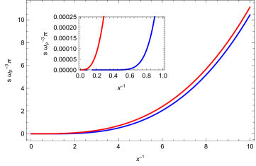
Figure 2: Comparison of the vacuum entropy density (59) (red curve)with the entropy density including plasma-model dispersion, (88), (blue curve). These are plotted as functions of $x^{-1}=2\pi T/\omega_{p}$. Both entropy densities tend to zero at zero temperature, and are everywhere positive. The inset shows the behavior for low temperature, and reveals that the plasma-model entropy drops exponentially to zero for relatively large values of the temperature.

Formal verification of this can be obtained by constructing a strong-coupling (low-temperature) expansion for the quantity in parentheses in Eq. (88) by the rest of the Bernoulli expansion,

$$s=\frac{\omega_{p}^{3}}{\pi}\int_{0}^{\infty}\frac{dy}{y}\sum_{k=3}^{\infty}\frac{B_{2k}}{2k!}\left(\frac{y}{x}\right)^{2k-1}J_{3}(y).$$ (89)

We use analytic continuation to define the $y$ integrals:

$$\int_{0}^{\infty}y^{2k-2}J_{3}(y)=2^{2k-2}\frac{\Gamma(1+k)}{\Gamma(3-k)},$$ (90)

which vanishes for $k\geq 3$. Thus, the low-temperature expansion of Eq. (88) is zero.

V.3.3 Strong-coupling, low-temperature, expansion

To verify this limiting behavior, let us try to extract directly the low-temperature (large $x$) limit. The Euler-Maclaurin formula should be effective in this regard:

$$\sum_{m=0}^{\infty}{}^{\prime}f(m)=\int_{0}^{\infty}dm\,f(m)-\sum_{k=1}^{\infty}\frac{B_{2k}}{(2k)!}f^{(2k-1)}(0),$$ (91)

where the prime means that the $m=0$ term is counted with half weight. For variety’s sake, let’s now set $\tau=0$, and keep only the spatial cutoff. Then the energy density (73) is

$$u=-\frac{T}{\pi\rho}\sum_{m=0}^{\infty}\zeta_{m}^{2}e^{-\rho\sqrt{\zeta_{m}^{2}+\omega_{p}^{2}}}=-\frac{T}{\pi\rho}\left(\frac{\partial^{2}}{\partial\rho^{2}}-\omega_{p}^{2}\right)\sum_{m=0}^{\infty}{}^{\prime}e^{-\rho\sqrt{\zeta_{m}^{2}+\omega_{p}^{2}}}.$$ (92)

The integral term in the Euler-Maclaurin formula gives

$$\int_{0}^{\infty}dm\,e^{-\rho\sqrt{(2\pi mT)^{2}+\omega_{p}^{2}}}=\frac{1}{2\pi T\rho}\int_{\omega_{p}\rho}^{\infty}du\frac{u}{\sqrt{u^{2}-\omega_{p}^{2}\rho^{2}}}e^{-u}=\frac{\omega_{p}}{2\pi T}K_{1}(\omega_{p}\rho).$$ (93)

Applying the differential operator in Eq. (92),

$$\left(\frac{\partial^{2}}{\partial\rho^{2}}-\omega_{p}^{2}\right)\frac{\omega_{p}}{2\pi T}K_{1}(\omega_{p}\rho)=\frac{\omega_{p}^{2}}{2\pi T\rho}K_{2}(\omega_{p}\rho),$$ (94)

and then using the small argument expansion of the modified Bessel function, we obtain for the integral contribution to the internal energy density

$$u_{\rm int}=-\frac{1}{\pi^{2}}\frac{1}{\rho^{4}}+\frac{1}{4\pi^{2}}\frac{\omega_{p}^{2}}{\rho^{2}}+\frac{\omega_{p}^{4}}{64\pi^{2}}\left(-3+4\gamma+4\ln(\omega_{p}\rho/2)\right).$$ (95)

This agrees with the $\tau=0$ divergences displayed in Eq. (74), while the logarithmic divergence in $\rho$ is the same as that in $\tau$ seen in Eq. (80).

But now it is apparently that $f(m)$ is an even function of $m$, which means that all the odd derivatives vanish. Thus, there is no temperature dependence of the internal energy in the low temperature limit. (That is, the dependence is exponentially small, and nonperturbative in the temperature.) This is consistent with the zero value of the entropy, without power corrections, found in this limit above.

V.3.4 Low-temperature asymptotics

In fact, we can readily obtain the asymptotic behavior for low temperature. We rewrite Eq. (92) as

$$u=\frac{T}{2\pi^{3/2}\rho}\left(\frac{\partial^{2}}{\partial\rho^{2}}-\omega_{p}^{2}\right)\frac{\partial}{\partial\rho}\rho\int_{0}^{\infty}dt\,t^{-3/2}e^{-t}e^{-\rho^{2}\omega_{p}^{2}/(4t)}\sum_{m=0}^{\infty}{}^{\prime}e^{-\rho^{2}\zeta^{2}_{m}/(4t)}.$$ (97)

Now, using the Poisson summation formula, we can recast the $m$ sum into Borwein and Borwein (1987)

$$\frac{1}{2}\sum_{m=-\infty}^{\infty}e^{-\rho^{2}\pi^{2}T^{2}m^{2}/t}=\frac{1}{\rho T}\sqrt{\frac{t}{\pi}}\sum_{m=0}^{\infty}{}^{\prime}e^{-m^{2}t/(\rho^{2}T^{2})}.$$ (98)

Then the $t$ integration gives a Macdonald function:

$$u=\frac{\omega_{p}^{4}}{2\pi^{2}}\frac{1}{\delta}\left(\frac{\partial^{2}}{\partial\delta^{2}}-1\right)\frac{\partial}{\partial\delta}\sum_{m=-\infty}^{\infty}K_{0}(\sqrt{\delta^{2}+(2\pi mx)^{2}}),$$ (99)

where $\delta=\omega_{p}\rho$. For $m=0$ this yields exactly the divergent structure (95) as $\delta\to 0$. However, for $m\neq 0$, the small $\delta$ limit is finite:

$$u_{m\neq 0}=\frac{\omega_{p}^{4}}{\pi^{2}}\sum_{m=1}^{\infty}\left[\frac{K_{1}(z)}{z}+\frac{3K_{2}(z)}{z^{2}}\right],\quad z=2\pi mx.$$ (100)

For large $z$, low temperature, this is dominated by the $m=1$ term,

$$u^{(1)}\sim\frac{\omega_{p}^{4}}{4\pi^{3}}x^{-3/2}e^{-2\pi x},\quad x\to\infty.$$ (101)

The entropy is obtained by integrating

$$\frac{\partial s}{\partial x}=\frac{2\pi x}{\omega_{p}}\frac{\partial u}{\partial x},$$ (102)

which yields the leading asymptotic approximation

$$s^{(1)}\sim\frac{\omega_{p}^{3}}{2\pi^{2}}\frac{e^{-2\pi x}}{\sqrt{x}},\quad T\ll\omega_{p}.$$ (103)

Comparisons with the exact results obtained from Eq. (86) are shown in Fig. 3. The exponential suppression of the entropy for temperatures low compared to the “mass,” the plasma frequency, is thus unambiguously established.

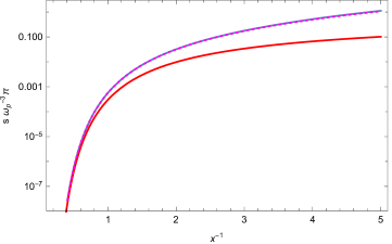
Figure 3: The exact entropy of the blackbody radiation in the plasma model (upper blue curve) compared with the leading low-temperature asymptotic expression (103) (lower red curve) and the numerical integration of the $m=1$ term in Eq. (100), dotted magenta curve. Even for $x=0.2$, a rather large value of $T$, the latter is less than 5% low. The cruder approximation (103) is only good for rather small values of $x^{-1}=2\pi T/\omega_{p}$.

V.3.5 Free energy

The above argument is defective in one sense: Because it was based on the internal energy, it did not determine the constant $s_{0}$ in the entropy, which had to be fixed by hand, by requiring that the entropy vanishes at zero temperature, the third law of thermodynamics. Therefore, it would appear more satisfactory to start with the free energy. However, this is more complex, as we now see.

The free energy is defined by

$$F=-\frac{T}{2}\operatorname{Tr}\ln\bm{\Gamma},$$ (104)

where the trace now includes the sum over Matsubara frequencies. Now from Eq. (68), we see that

$$0=\frac{\partial}{\partial\omega_{p}^{2}}\left(\bm{\Gamma}^{-1}\bm{\Gamma}\right)=-\frac{1}{\zeta_{m}^{2}}\bm{\Gamma}+\frac{\partial}{\partial\omega_{p}^{2}}\ln\bm{\Gamma},$$ (105)

which says that

$$\ln\bm{\Gamma}(\omega_{p}^{2})=-\frac{1}{\zeta_{m}^{2}}\int_{\omega_{p}^{2}}^{\infty}d\omega_{p}^{\prime 2}\,\bm{\Gamma}(\omega_{p}^{\prime 2}).$$ (106)

Now the internal energy is proportional to the trace of $\bm{\Gamma}$, so the free energy can be immediately given after integration on $\omega_{p}^{\prime 2}$ as

$$f=-\frac{T}{\pi\rho^{2}}\sum_{m=0}^{\infty}{}^{\prime}\left(\sqrt{\zeta_{m}^{2}+\omega_{p}^{2}}+\frac{1}{\rho}\right)e^{-\rho\sqrt{\zeta_{m}^{2}+\omega_{p}^{2}}}.$$ (107)

When $\omega_{p}^{2}=0$, this directly implies Eq. (59).

In general, we have to consider $m=0$ separately from the higher Matsubara terms. (Recall, $m=0$ does not contribute to the internal energy.) That is

$$f_{m=0}=\frac{T}{2\pi\rho^{2}}\left(\frac{\partial}{\partial\rho}-\frac{1}{\rho}\right)e^{-\rho\omega_{p}}\sim-\frac{T}{2\pi\rho^{3}}+\frac{T\omega_{p}^{2}}{4\pi\rho}-\frac{T\omega_{p}^{3}}{6\pi},\quad\rho\to 0.$$ (108)

The $T$-dependent divergent terms must be cancelled by the remainder of the Matsubara series. As before, we can proceed perturbatively in powers of $\omega_{p}$. The zeroth order term is

$$f^{(0)}_{m\neq 0}=\frac{T}{\pi\rho^{2}}\left(\frac{\partial}{\partial\rho}-\frac{1}{\rho}\right)\sum_{m=1}^{\infty}e^{-2\pi mT\rho}\sim-\frac{1}{\pi^{2}\rho^{2}}+\frac{T}{2\pi\rho^{3}}-\frac{\pi^{2}T^{4}}{45},\quad\rho\to 0$$ (109)

where the first and last terms reproduce Eq. (59) and the middle term cancels the $\omega_{p}$-independent term in Eq. (108).

The term of order $\omega_{p}^{2}$ is

$$f^{(1)}_{m\neq 0}=\frac{\omega_{p}^{2}T}{2\pi\rho}\sum_{m=1}^{\infty}e^{-\rho\zeta_{m}}\sim\frac{\omega_{p}^{2}}{4\pi\rho^{2}}-\frac{\omega_{p}^{2}T}{4\pi\rho}+\frac{\omega_{p}^{2}T^{2}}{12},\quad\rho\to 0.$$ (110)

The second term here cancels the second term in Eq. (108), and we are left with the structure seen in Eqs. (74) and (75). As for the term of order $\omega_{p}^{4}$, we have

$$f_{m\neq 0}^{(2)}=-\frac{\omega_{p}^{4}}{16\pi^{2}}\sum_{m=1}^{\infty}\frac{1}{m}e^{-\delta m/x}\sim\frac{\omega_{p}^{4}}{16\pi^{2}}\ln 2\pi T\rho,$$ (111)

again as anticipated.

Since this approach seems a bit complicated, we will reinsert a temporal regulator, which simplifies the calculation. But we have already achieved our goal: It is clear that the perturbative expansion for $m\neq 0$ contributions involves only even powers of $\omega_{p}$, so the only term of order $\omega_{p}^{3}$ is that remaining in Eq. (108). This term, linear in the temperature, corresponds to the constant term in the entropy, undetermined by the previous analysis:

$$s_{0}=\frac{\omega_{p}^{3}}{6\pi}.$$ (112)

Naively inserting the temporal regulator into Eq. (107), we write

$$f=\frac{T}{2\pi\rho^{2}}\left(\frac{\partial}{\partial\rho}-\frac{1}{\rho}\right)\sum_{m=-\infty}^{\infty}e^{-\rho\sqrt{\zeta_{m}^{2}+\omega_{p}^{2}}}e^{i\zeta_{m}\tau}.$$ (113)

Now with $\tau\neq 0$, we can expand in $\rho$, and after omitting terms involving $\delta$ functions in $\tau$, find

$$f=-\frac{T}{6\pi}\sum_{m=-\infty}^{\infty}(\zeta_{m}^{2}+\omega_{p}^{2})^{3/2}e^{i\zeta_{m}\tau}.$$ (114)

Now, this is readily expanded in powers of $x=\omega_{p}/\zeta_{1}$. Following the by-now familiar procedure, we find the first three divergent terms:

$$f^{(0)} = -\frac{1}{\pi^{2}\tau^{4}}-\frac{\pi^{2}T^{4}}{45},$$ (115a)

$$f^{(1)} = \frac{\omega_{p}^{2}}{4\pi^{2}\tau^{2}}+\frac{\omega_{p}^{2}}{12}T^{2},$$ (115b)

$$f^{(2)} = \frac{\omega_{p}^{4}}{16\pi^{2}}\ln 2\pi T\tau.$$ (115c)

The remaining terms are finite. The only odd term in $\omega_{p}$ comes from the $m=0$ term:

$$f_{m=0}=-\frac{\omega_{p}^{3}T}{6\pi},$$ (116)

which corresponds precisely to the constant term in the entropy. Then, the higher terms in $\omega_{p}$ are

$$f^{(k\geq 3)}=\frac{8\pi^{2}T^{4}}{3}\frac{\Gamma(5/2)\zeta(2k-3)}{\Gamma(k+1)\Gamma(5/2-k)}x^{2k},$$ (117a)

corresponding to the entropy term

$$s^{(k\geq 3)}=4\pi^{5/2}T^{3}\frac{(2-k)\zeta(2k-3)}{\Gamma(k+1)\Gamma(5/2-k)}x^{2k}.$$ (117b)

The temperature-dependence of $f$, and the entropy are precisely those found previously in Sec. V.3.1. The cutoff terms, however, are off by $-\frac{1}{3}$ and $-1$ for the quartically divergent and quadratically terms, respectively. This is due, as explained in Ref. Parashar et al. (2017), to the fact that an exponential temporal cutoff in the free energy corresponds to a more elaborate form for the internal energy:

$$e^{i\zeta\tau}\to\frac{e^{i\zeta\tau}-1}{i\zeta\tau}$$ (118)

This precisely accounts for the discrepant factors in the zero-temperature divergences.

VI Conclusions

Previously Milton et al. (2017b, 2019); Li et al. (2021), we analyzed the self-entropy of a macroscopic sphere. But viewed from far away, a compact object appears to be a particle. So, in this paper, we examine the question of self-entropy from the nanoparticle perspective. By nanoparticle, we mean that the size of the particle is small compared to any other length scale, such as the inverse temperature. This self-entropy exhibits surprising features, especially its negativity for weak coupling to the electromagnetic field. We approach this question by first extracting the polarizabilities of a nanoparticle through consideration of its effect on the scattering of the electromagnetic field. From these polarizabilities, expressed in terms of the reflection coefficients, we can compute the free energy and entropy by summing over Matsubara frequencies. The results apply to low temperatures, compared to the inverse size of the nanoparticle. (For a 100 nm particle, the temperature for which $aT=1$ is 24,000 K.)

Specifically, we illustrate these ideas by investigating two models. First, for a $\delta$-function spherical shell in which the permittivity on the surface is transverse and represented by the plasma model, we obtain results for the self-entropy which give the leading low-temperature response, linear in the coupling, for the TE and TM modes; these self-entropies are precisely those found earlier Milton et al. (2017b). The second model, a dielectric/diamagnetic ball without dispersion, involves more subtleties. The scattering-derived polarizabilities give a contribution to the free energy which is linear in the susceptibility, in the dilute limit, which therefore violates the expected connection between Casimir and van der Waals forces Milton et al. (2020).

This discrepancy is resolved by the subtraction of the “bulk contribution,” which is the contribution to the Casimir free energy corresponding to the nonscattering Green’s functions due to the medium either inside or outside the spherical boundary filling the whole space. (Such a contribution only removes the vacuum contribution for a hollow spherical shell.) Performing this subtraction, we remove the linear term, and recover the negative self-entropy found two decades ago Barton (2001b, a); Nesterenko et al. (2001). That self-entropy is reproduced again in Appendices A–C.

However, the reader might well object to the fact that the known energies at zero temperature are not reproduced by the procedure proposed here. After all, in second order in the susceptibility, the finite part of the energy of the dielectric ball is as given by the first term in Eq. (41). But here the only finite terms in the free energy are those going like a power of the temperature, yielding a finite self-entropy. Furthermore, the divergent term found here for the dielectric ball is the difference between the $\tau$-dependent terms in Eqs. (39) and (50),

$$F_{\rm div}=\frac{7a^{3}}{6\pi\tau^{4}}(\varepsilon-1)^{2},$$ (119)

while the energy found some forty years ago Milton (1980) is less singular,

$$E_{\rm div}=\frac{a^{2}}{8\tau^{3}}(\varepsilon-1)^{2}.$$ (120)

One might think that the reason for not seeing the temperature-independent finite terms is that extraction of these requires more sophisticated analytic continuation techniques, such as zeta-function regularization, which sweep divergences under the rug. Apparently, the point-particle viewpoint is only effective in extracting the temperature-dependent part of the free energy, and therefore the entropy, but not the finite or divergent parts. As argued in Appendix B, it would be anticipated that the point-particle viewpoint being explored here is only effective in extracting extensive quantities, proportional to the volume of the particle, and not contributions to the free energy going like lower powers of the radius of the particle.

On the other hand, we now understand the appearance of negative self-entropies found for objects, be they macroscropic dielectric balls or small nanoparticles. The approach presented here reveals the negative entropy as arising from an interaction between the nanoparticle and the blackbody radiation. As discussed in Appendix B, the free energy of the blackbody radiation in vacuum, and in the material of the dielectric ball, both without interaction (that is, the “nonscattering” part), must be subtracted from the total free energy to obtain the self-free energy, or the interaction free energy. This precisely corresponds to our bulk subtraction. The resulting interaction entropy can be, in fact, negative. (It bears a resemblance to, but in general, is not the same as, the negative of the relative entropy discussed in Ref. Breuer and Petruccione (2002).) The total entropy, of course, has the bulk, blackbody entropies included, so is always positive.

Appendix A Bulk Subtraction at Finite Temperature

It might be thought that the bulk subtraction, which we used to derive the entropy of the dielectric/diamagnetic ball, need only be employed at zero temperature. After all, the bulk divergences occur only at zero temperature. But this is not correct, because the reason for the subtraction is not primarily to remove divergences, but to remove the effects of a homogeneous medium, the non-scattering contribution of the Green’s function to the internal energy. We see this in the general formula (66), from which the zero-temperature form for the energy is obtained, for example, by the Euler-Maclaurin summation formula. This involves all $m$, so the replacement of the Green’s dyadic by its scattering part must be applied universally. The subtraction is not required in order to make the energy finite (which it is not, even after this truncation of the Green’s function), but because it is necessary physically: the Casimir-Lifshitz energy must arise, at least in the dilute approximation, from the summation of van der Waals or Casimir-Polder interactions, which are quadratic in the polarizability, so the Casimir-Lifshitz free energy at arbitrary temperature must start from order $(\varepsilon-1)^{2}$ for a dilute dielectric sphere. All of this was recognized by Dzyaloshinskii, Lifshitz, and Pitaevskii Dzyaloshinskii et al. (1961), and constitutes the “Lifshitz subtraction.”

A.1 Casimir-Polder Free Energy of Two Dilute Dielectric Slabs

We can demonstrate this explicitly by considering the classic Lifshitz configuration Lifshitz (1956) of two parallel dielectric slabs separated by a vacuum region of width $a$. In the limit where the two dielectric media are dilute, we can compute this in two ways: either by summing the van der Waals interactions between the various atoms constituting the slabs, or by taking the dilute limit of the Lifshitz free energy. Let’s consider the high-temperature limit, and suppose that the Casimir-Polder interaction Casimir and Polder (1948) between atoms with polarizability $\alpha_{1}$ and $\alpha_{2}$ separated by a distance $r$ is in the classical limit

$$V=-CT\frac{\alpha_{1}\alpha_{2}}{r^{6}},$$ (121)

a structure required dimensionally, where $C$ is a dimensionless constant to be determined. The free energy of the two slabs is obtained by summing the interactions between the two slabs, which are supposed to be homogeneous, with number densities $N_{1}$ and $N_{2}$. The free energy is

$$F_{\rm CP}=-CTN_{1}\alpha_{1}N_{2}\alpha_{2}\int_{-\infty}^{0}dz\int_{a}^{\infty}dz^{\prime}\int(d\mathbf{r}_{\perp})(d\mathbf{r^{\prime}}_{\perp})\left[(\mathbf{r_{\perp}-r^{\prime}_{\perp}})^{2}+(z-z^{\prime})^{2}\right]^{-3}.$$ (122)

The integrations are elementary, leading to the free energy per unit area

$$\frac{F_{\rm CP}}{A}=-CT\frac{\pi}{12}\frac{N_{1}N_{1}\alpha_{1}\alpha_{2}}{a^{2}}.$$ (123)

The bulk-subtracted Lifshitz pressure between the two slabs is Lifshitz (1956); Schwinger et al. (1978)

$$p=-\frac{T}{8\pi}\sum_{m=-\infty}^{\infty}\int_{0}^{\infty}dk^{2}\,2\kappa_{3}\left(\frac{1}{\Delta^{E}}+\frac{1}{\Delta^{H}}\right),$$ (124)

for the configuration where the top and bottom slabs are denoted 1 and 2, and the intermediate vacuum region is denoted 3. The denominators are, in terms of the inverses of the reflection coefficients at the interfaces,

$$\Delta^{E} = \frac{\kappa_{3}+\kappa_{1}}{\kappa_{3}-\kappa_{1}}\frac{\kappa_{3}+\kappa_{2}}{\kappa_{3}-\kappa_{2}}e^{2\kappa_{3}a}-1,$$ (125a)

$$\Delta^{H} = \frac{\kappa_{3}/\varepsilon_{3}+\kappa_{1}/\varepsilon_{1}}{\kappa_{3}/\varepsilon_{3}-\kappa_{1}/\varepsilon_{1}}\frac{\kappa_{3}/\varepsilon_{3}+\kappa_{2}/\varepsilon_{2}}{\kappa_{3}/\varepsilon_{3}-\kappa_{2}/\varepsilon_{2}}e^{2\kappa_{3}a}-1,$$ (125b)

where

$$\kappa_{3}=\kappa=\sqrt{k^{2}+\zeta_{m}^{2}},\quad\kappa_{1,2}=\sqrt{k^{2}+\varepsilon_{1,2}(\zeta_{m})\zeta_{m}^{2}}.$$ (126)

When $\varepsilon_{1,2}-1$ are both small, this is readily expanded to the leading order: introducing the variable $u=\kappa/\zeta_{m}$, we have

$$p=-\frac{T}{16\pi}\sum_{m=0}^{\infty}\!{}^{\prime}\zeta_{m}^{3}(\varepsilon_{1}(\zeta_{m})-1)(\varepsilon_{2}(\zeta_{m})-1)\int_{1}^{\infty}\frac{du}{u^{2}}[1+(1-2u^{2})^{2}]e^{-2\zeta_{m}ua}.$$ (127)

Now we are interested in high temperature, which corresponds to $m=0$, so we take the limit of small $\zeta_{m}$. In that limit, the $u$ integral is asymptotically $(\zeta_{m}a)^{-3}$, and then the $m=0$ term in the free energy, obtained by integrating

$$p=-\frac{\partial}{\partial a}\frac{F}{A}$$ (128)

is, in terms of the static dielectric constants

$$\frac{F}{A}=-\frac{T}{64\pi}(\varepsilon_{1}-1)(\varepsilon_{2}-1)\frac{1}{a^{2}},\quad aT\gg 1.$$ (129)

These two expressions, Eq. (129) and Eq. (123), should be identical. They are, when we recall the connection between the dielectric constant and the polarizability:

$$\varepsilon=1+N\alpha,$$ (130)

and this determines the constant in the van der Waals potential to be $C=3/(4\pi)^{2}$.

A.2 Casimir-Polder Free Energy of Dilute Dielectric Ball

We can straightforwardly extend this argument to sum the Casimir-Polder energies of the atomic constituents of a dilute dielectric sphere. This should correspond to the free energy of such an object. Such a calculation, in fact, is the same idea as that exploited by Barton Barton (2001a), although the calculational details are different, as are the results.

The free energy of interaction between the constituents of isotropic polarizability $\alpha$ is given by Milton et al. (2015)

$$F_{CP}=-\frac{1}{2}\frac{N^{2}\alpha^{2}}{(4\pi)^{2}}\int(d\mathbf{r})(d\mathbf{r^{\prime}})\frac{1}{4\pi\rho^{7}}f(y),$$ (131)

where $y=4\pi\rho T$, $\rho=\sqrt{r^{2}-r^{\prime 2}-\mathbf{r\cdot r^{\prime}}}$, and

$$f(y)=yD_{T}\coth\frac{y}{2},$$ (132a)

with

$$D_{T}=3-3T\partial_{T}+\frac{5}{4}T^{2}\partial_{T}^{2}-\frac{1}{4}T^{3}\partial_{T}^{3}+\frac{1}{16}T^{4}\partial_{T}^{4}.$$ (132b)

(Note, at high $T$, where $\coth y/2$ tends to 1, this yields Eq. (121) with $C=3/(4\pi)^{2}$.) Here $N$ is the number density of polarizable constituents. The integrals extend over the volume of the sphere wherein the constituents reside. Since $\rho$ never gets large, to extract the low-temperature behavior, we can expand the hyperbolic cotangent for small argument:

$$\coth z=\frac{1}{z}+\frac{z}{3}-\frac{z^{3}}{45}+\frac{2z^{5}}{45}+\dots.$$ (133)

Consider the first term in the expansion. Since the differential operator $D_{T}$ applied to $1/T$ yields $\frac{23}{2T}$, we are left with evaluating the radial integral

$$\int(d\mathbf{r})(d\mathbf{r^{\prime}})\frac{1}{\rho^{7}}.$$ (134)

This integral is divergent, because the coordinates can be coincident, but a method of extracting the finite part was described in Refs. Milton and Ng (1998); Milton (2001). Let’s consider the generic integral

$$I(\gamma)=\int(d\mathbf{r})(d\mathbf{r^{\prime}})\frac{1}{\rho^{\gamma}}.$$ (135)

The result is, for $\gamma<3$,

$$I(\gamma)=\frac{128\pi^{2}2^{-\gamma}}{(6-\gamma)(4-\gamma)(3-\gamma)}a^{6-\gamma}.$$ (136)

This integral is well defined if $\gamma$ is 7, so by analytic continuation we immediately obtain the zero temperature free energy

$$E_{0}=\frac{23}{1536}\frac{(\varepsilon-1)^{2}}{\pi a},$$ (137)

where we identify $\varepsilon-1=N\alpha$. This is the well-known result Milton and Ng (1998), seen in Eq. (41),

As for the low temperature corrections, it is apparent that the differential operator $D_{T}$ annihilates a term linear in $T$, so the $O(z)$ term in the expansion of the cotangent is without effect because $I(5)$ is finite. $D_{T}$ has the same effect on the $T^{3}$ term. But that corresponds to $\gamma=3$, where the volume integral (136) has a pole, so we must take a limit. Write $y^{3}\to y^{3-s}$ where $s\to 0$. So then

$$D_{T}T^{3-s}\to-\frac{7}{8}sT^{3},\quad s\to 0,$$ (138)

while

$$I(3+s)\to-\frac{16\pi^{2}}{3s}a^{3},$$ (139)

so the product is finite as $s\to 0$, and supplying the other factors, we obtain for the temperature correction to the free energy

$$\Delta F_{T}=\frac{7}{270}(\varepsilon-1)^{2}(\pi a)^{3}T^{4},$$ (140)

precisely the result (41) given by Nesterenko et al. Nesterenko et al. (2001) but without the additional $T^{3}$ term found by Barton Barton (2001a).

Appendix B Sign of the Interaction Entropy for a Dielectric Ball

In this appendix, we explore the sign of the interaction entropy for a dielectric ball, using the Clausius-Mossotti relation Schwinger et al. (1998). We begin with a critical appraisal of the approximation of the finite-size nanoparticle by a point particle with the same polarizability, and an appreciation of the limitations of this approximation.

The use of Eq. (25) in Eq. (24) implies a resummation of the usual perturbative expansion to all orders in $\varepsilon-1$, to extract all contributions to leading order in the particle size, which, in total, give rise to its polarizability. By construction, therefore, this procedure can only produce the extensive contribution to the free energy of the nanoparticle, that is, that part of the free energy that is proportional to the volume of the nanoparticle. It cannot capture any other contributions to the free energy that are not extensive, such as the surface term obtained by Barton Barton (2001b), or the zero-temperature term displayed in Eq. (41), which is proportional to the inverse radius of the nanoparticle Nesterenko et al. (2001); Barton (2001b, a); Milton and Ng (1998); Brevik et al. (1999), or, indeed, any contributions that are of higher order in the polarizability. Likewise, only the extensive contribution to the corresponding derived entropy can result. This is a fundamental limitation of the approximation employed.

In this approximation, the free energy, $F$, of the nanoparticle may be regarded as a linear function of the extensive variable, $V$, the volume of the nanoparticle, and a possibly nonlinear function of the intensive variable, $N$, the number density of its polarizable constituents. Below, we explore the assembly of the nanoparticle from its initially widely-dispersed constituents, and so are interested in how the free energy changes with the volume, while keeping the number of constituents fixed. Since

$$\frac{dF}{dV}=\frac{\partial F}{\partial V}-\frac{N}{V}\frac{\partial F}{\partial N}=\frac{F}{V}-\frac{N}{V}\frac{\partial F}{\partial N},$$ (141)

it follows that $\frac{dF}{dV}=0$, that is, the free energy of the nanoparticle is invariant under this change in volume, if and only if it is also a linear function of $N$. In fact, this is the case for the Clausius-Mossotti relation, which expresses the polarizability of a dielectric ball as a linear function of the number density, and polarizability, of its constituents. It should be noted that linearity in the number density of the constituents does not preclude interaction between these constituents. Indeed, the Clausius-Mossotti relation derives from the inclusion of the effect on the induced dipole moment of each constituent of the induced electric field due to the induced dipole moments of the other constituents. This interaction between the constituents is reflected in the nonlinear dependence of the polarizability on $\varepsilon-1$.

To be specific, let us therefore assume that the permeability $\mu=1$ and that the system consists of a dielectric ball, $B$, of radius $a$ and permittivity $\varepsilon$, which is composed of polarizable constituents of number density $N$ and polarizability $\alpha_{c}$, and which is surrounded by vacuum. Let us also consider the corresponding reference system which consists of the dilated ball, $B_{\lambda}$, of radius $\lambda a$ and permittivity $\varepsilon_{\lambda}$, wherein the polarizable constituents have number density $N_{\lambda}\equiv\frac{N}{\lambda^{3}}$, where $\lambda>1$, which is also surrounded by vacuum. From the Clausius-Mossotti relation, we immediately obtain the relation between the corresponding permittivities:

$$\frac{\varepsilon-1}{\varepsilon+2}=\frac{N\alpha_{c}}{3}=\frac{\lambda^{3}N_{\lambda}\alpha_{c}}{3}=\lambda^{3}\left(\frac{\varepsilon_{\lambda}-1}{\varepsilon_{\lambda}+2}\right).$$ (142)

The total free energy of the original system may be constructed from three components,

$$F_{\text{tot}}=F_{\text{vac}}^{{\mathbb{R}}^{3}}+\left(F_{\text{med}}^{B}-F_{\text{vac}}^{B}\right)+F_{\text{int}}^{B},$$ (143)

using an obvious notation: $F_{\text{med}}^{B}-F_{\text{vac}}^{B}$ is the change in the bulk free energy of the ball resulting from replacement of vacuum by medium in its interior, which arises from the corresponding change in the non-scattering part of the Green’s function, and $F_{\text{int}}^{B}$ is the interaction free energy between the interior of the ball (medium) and its exterior (vacuum), which arises from the scattering part of the corresponding Green’s function. Likewise, the total free energy of the reference system may be written as

$$F_{\text{tot}}^{\lambda}=F_{\text{vac}}^{{\mathbb{R}}^{3}}+\left(F_{\text{med}}^{B_{\lambda}}-F_{\text{vac}}^{B_{\lambda}}\right)+F_{\text{int}}^{B_{\lambda}}.$$ (144)

The change in the bulk free energy of the dilated ball is

$$F_{\text{med}}^{B_{\lambda}}-F_{\text{vac}}^{B_{\lambda}}=\int_{B_{\lambda}}d\mathbf{r}\left(\varepsilon_{\lambda}^{\frac{3}{2}}-1\right)f_{0}(\tau,T)=\frac{4}{3}\pi a^{3}\lambda^{3}\left[\left(\frac{1+\frac{2N\alpha_{c}}{3\lambda^{3}}}{1-\frac{N\alpha_{c}}{3\lambda^{3}}}\right)^{\!\!\frac{3}{2}}-1\right]f_{0}(\tau,T),$$ (145)

which becomes, in the limit $\lambda\to\infty$,

$$\lim_{\lambda\to\infty}\left(F_{\text{med}}^{B_{\lambda}}-F_{\text{vac}}^{B_{\lambda}}\right)=\frac{4}{3}\pi a^{3}\,\frac{9}{2}\left(\frac{\varepsilon-1}{\varepsilon+2}\right)f_{0}(\tau,T),$$ (146)

where

$$f_{0}(\tau,T)\equiv-\frac{1}{\pi^{2}\tau^{4}}-\frac{\pi^{2}T^{4}}{45}$$ (147)

is the vacuum free energy density (115a) under the temporal regulator $\tau$. As expected, this is simply the sum over the finite number, $\frac{4}{3}\pi a^{3}N$, of the then infinitely separated and therefore non-interacting polarizable constituents, each of which contributes $\frac{3}{2}\alpha_{c}f_{0}(\tau,T)$ to the free energy. Correspondingly, in this limit, the interaction free energy of the dilated ball must vanish, as it then fills all space and has no exterior, so $\lim_{\lambda\to\infty}F_{\text{int}}^{B_{\lambda}}=0$. (See below.)

Thus,

$$\left(F_{\text{med}}^{B}-F_{\text{vac}}^{B}\right)-\lim_{\lambda\to\infty}\left(F_{\text{med}}^{B_{\lambda}}-F_{\text{vac}}^{B_{\lambda}}\right)=\frac{4}{3}\pi a^{3}\left[\varepsilon^{\frac{3}{2}}-1-\frac{9}{2}\left(\frac{\varepsilon-1}{\varepsilon+2}\right)\right]f_{0}(\tau,T).$$ (148)

This expression represents the change in the total bulk free energy when the ball is assembled from its initially maximally dispersed constituents, and its sign is determined from that of

$$g(\varepsilon)\equiv\varepsilon^{\frac{3}{2}}-1-\frac{9}{2}\left(\frac{\varepsilon-1}{\varepsilon+2}\right).$$ (149)

It is easily verified that $g(1)=0$ and $g(\varepsilon)>0$ for $\varepsilon>0$, $\varepsilon\neq 1$. Therefore, the change in the total bulk free energy is negative, and, correspondingly, from Eq. (147), the change in the total bulk entropy is positive.

However, Eq. (148) may also be written as $\left(F_{\text{tot}}-F_{\text{int}}^{B}\right)-\left(F_{\text{tot}}^{\infty}-\lim_{\lambda\to\infty}F_{\text{int}}^{B_{\lambda}}\right)=-F_{\text{int}}^{B}$, since $\lim_{\lambda\to\infty}F_{\text{int}}^{B_{\lambda}}=0$ and $F_{\text{tot}}=F_{\text{tot}}^{\infty}$, the latter because of the linear dependence of the free energy of the dielectric ball on the number density of its polarizable constituents, inherited from the Clausius-Mossotti relation, as described in Eq. (141). Thus,

$$F_{\text{int}}^{B}=\frac{4}{3}\pi a^{3}\left[\frac{9}{2}\left(\frac{\varepsilon-1}{\varepsilon+2}\right)-\left(\varepsilon^{\frac{3}{2}}-1\right)\right]f_{0}(\tau,T)=-\frac{4}{3}\pi a^{3}g(\varepsilon)\,f_{0}(\tau,T)>0$$ (150a)

and, correspondingly,

$$S_{\text{int}}^{B}=\left[\frac{9}{2}\left(\frac{\varepsilon-1}{\varepsilon+2}\right)-\left(\varepsilon^{\frac{3}{2}}-1\right)\right]\frac{2t^{3}}{135}=-g(\varepsilon)\frac{2t^{3}}{135}<0,\quad t=2\pi aT.$$ (150b)

That is, the ball has a positive interaction free energy and a corresponding negative interaction entropy.

From Eq. (150a), we can demonstrate self-consistency by noting that the interaction free energy of the dilated ball vanishes as the dilation factor goes to infinity:

$$F_{\rm int}^{B_{\lambda}}=-\frac{4\pi(\lambda a)^{3}}{3}\left[\varepsilon_{\lambda}^{3/2}-1-\frac{9}{2}\frac{\varepsilon_{\lambda}-1}{\varepsilon_{\lambda}+2}\right]f_{0}(\tau,T)\to-\frac{\pi a^{3}}{2}\frac{N^{2}\alpha_{c}^{2}}{\lambda^{3}}f_{0}(\tau,T)\to 0,\quad\lambda\to\infty.$$ (151)

The important point to note here is that, because, under the Clausius-Mossotti relation, the total free energy of the system is unchanged when the ball is assembled from its initially maximally dispersed and therefore non-interacting constituents, the decrease in the total bulk free energy resulting from the assembly is exactly offset by a corresponding increase in the initially vanishing interaction free energy, resulting here in a positive interaction free energy and a corresponding negative interaction entropy for the ball. The assembly of the ball from its constituents would otherwise be a spontaneous process, decreasing the total bulk free energy and increasing the total bulk entropy. However, the assembly itself creates the differentiation between the interior (medium) and the exterior (vacuum) of the ball, and the resulting macroscopic inhomogeneity in the permittivity gives rise to the scattering part of the Green’s function and the corresponding inhibiting positive interaction free energy and negative interaction entropy. In this point of view, the appearance of a negative interaction entropy is seen as a natural and inevitable consequence of the creation of the scattering contribution to the Green’s function through the assembly process. (Of course, this conclusion only holds for $\mu=1$.)

In spite of the negative interaction entropy, insertion of the particle into the vacuum always decreases (if $\varepsilon>1$) the total free energy and increases the total entropy of the system:

$$F_{\text{tot}}-F_{\text{vac}}^{{\mathbb{R}}^{3}}=\left(F_{\text{med}}^{B}-F_{\text{vac}}^{B}\right)+F_{\text{int}}^{B}=6\pi a^{3}\left(\frac{\varepsilon-1}{\varepsilon+2}\right)f_{0}(\tau,T)<0$$ (152a)

and

$$S_{\text{tot}}-S_{\text{vac}}^{{\mathbb{R}}^{3}}=\left(S_{\text{med}}^{B}-S_{\text{vac}}^{B}\right)+S_{\text{int}}^{B}=\left(\frac{\varepsilon-1}{\varepsilon+2}\right)\frac{t^{3}}{15}>0.$$ (152b)

More generally, the interaction entropy could be of either sign. If the ball has permeability as well as permittivity, the interaction entropy becomes

$$S_{\rm int}=-g(\varepsilon,\mu)\frac{2t^{3}}{135},\quad g(\varepsilon,\mu)=(\varepsilon\mu)^{3/2}-1-\frac{9}{2}\left(\frac{\varepsilon-1}{\varepsilon+2}+\frac{\mu-1}{\mu+2}\right).$$ (153)

A perfectly conducting spherical shell corresponds to $\varepsilon\to\infty$, $\mu\to 0$ so that $\varepsilon\mu\to 1$. (The latter corresponds to the interior of the shell being vacuum as in the exterior.) In this way the familiar result (31) emerges,

$$S_{\rm PCS}=\frac{t^{3}}{30},$$ (154)

which is positive. But it is not necessary to go to the limit to see the change in sign. Although the interaction entropy (153) is nonpositive whenever $\varepsilon$ and $\mu$ are both $\geq 1$, if one of these is less than unity, there is a region of positive entropy, as illustrated in Fig. 4.

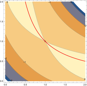
Figure 4: The entropy given in terms of $-g(\varepsilon,\mu)$ in Eq. (153) for $\varepsilon$ and $\mu$ between $0$ and $2$. The contour lines denote the boundaries of regions where the function has values between the designated integers. The positive entropy region is colored lightest (yellow), roughly following the $\varepsilon\mu=1$ hyperbola shown in red.

Appendix C Direct Calculation of Low-Temperature Correction to Interaction Free Energy

It is easy to obtain the general results for the low-temperature correction to the free energy, and the low-temperature entropy, directly from the zero-temperature expressions derived many years ago Milton (1980); Milton and Ng (1997); Milton (2001). The pressure on a dielectric/diamagnetic ball is given there by

$$p=\frac{1}{2a^{3}}\int_{-\infty}^{\infty}\frac{d\zeta}{2\pi}e^{i\zeta\tau}\sum_{l=1}^{\infty}\frac{2l+1}{4\pi}\left[f_{l}(x)-f^{(0)}_{l}(x)\right],$$ (155)

where the contribution from the bulk subtraction is

$$f^{(0)}_{l}(x)=2x[s^{\prime}_{l}(x)e_{l}^{\prime}(x)-e_{l}(x)s_{l}^{\prime\prime}(x)]-2x^{\prime}[s^{\prime}_{l}(x^{\prime})e_{l}^{\prime}(x^{\prime})-e_{l}(x^{\prime})s_{l}^{\prime\prime}(x^{\prime})],$$ (156a)

where $$x=|\zeta|a x^{\prime}=\sqrt{\varepsilon\mu}x$$, , and the scattering contribution is

$$f_{l}(x)=x\frac{d}{dx}D_{l}(x),\quad D_{l}(x)=[s_{l}(x^{\prime})e_{l}^{\prime}(x)-s_{l}^{\prime}(x^{\prime})e_{l}(x)]^{2}-\xi^{2}[s_{l}(x^{\prime})e_{l}^{\prime}(x)+s_{l}^{\prime}(x^{\prime})e_{l}(x)]^{2},$$ (156b)

with

$$\xi=\frac{\sqrt{\frac{\varepsilon}{\mu}}-1}{\sqrt{\frac{\varepsilon}{\mu}}+1}.$$ (157)

To extend these old results to finite temperature, we simply replace the integral over Euclidean frequencies by a sum over Matsubara frequencies:

$$\int_{-\infty}^{\infty}\frac{d\zeta}{2\pi}\to T\sum_{m=-\infty}^{\infty},\quad\zeta\to\zeta_{m}=2\pi mT.$$ (158)

For low temperatures, we can evaluate the sum by using the Euler-Maclaurin sum formula (91). The integral there, of course, corresponds to the original zero-temperature result, which contains all the divergences. The sum over Bernoulli numbers contains the finite temperature corrections, which must be understood as an asymptotic series. So we need the odd derivatives of $f_{l}$ and $f_{l}^{(0)}$ at zero to find the temperature corrections, which requires computing the odd terms in the power series expansion of these functions about the origin. The leading power, as would have been anticipated Milton et al. (2017b), occurs only for $l=1$:

$$f_{1}(x)\sim-2x^{3}\left(\frac{\varepsilon-1}{\varepsilon+2}+\frac{\mu-1}{\mu+2}\right),\quad f_{1}^{(0)}(x)\sim\frac{4}{9}x^{3}\left(1-(\varepsilon\mu)^{3/2}\right),\quad x\ll 1.$$ (159)

Supplying the remaining factors, we immediately obtain the small temperature correction to the pressure,

$$\Delta P=-\frac{\pi^{2}T^{4}}{45}g(\varepsilon,\mu).$$ (160)

Since $4\pi a^{2}p=-\frac{\partial}{\partial a}F$, the temperature correction to the free energy is just as found above,

$$\Delta F=\frac{4\pi a^{3}}{3}\frac{\pi^{2}T^{4}}{45}g(\varepsilon,\mu),$$ (161)

and the entropy (153) follows. This elementary calculation should have been done 40 years ago.

References

- Bezerra et al. (2004) V. B. Bezerra, G. L. Klimchitskaya, V. M. Mostepanenko, and C. Romero, “Violation of the Nernst heat theorem in the theory of the thermal Casimir force between Drude metals,” Phys. Rev. A 69, 022119 (2004).
- Klimchitskaya and Korikov (2015) G. L. Klimchitskaya and C. C. Korikov, “Casimir entropy for magnetodielectrics,” J. Phys. Condens. Matter 27, 214007 (2015).
- Korikov (2016) C. C. Korikov, “Casimir entropy for ferromagnetic materials,” Int. J. Mod. Phys. A 31, 1641036 (2016).
- Klimchitskaya and Mostepanenko (2017) G. L. Klimchitskaya and V. M. Mostepanenko, “Low-temperature behavior of the Casimir free energy and entropy of metallic films,” Phys. Rev. A 95, 012130 (2017).
- Brevik et al. (2006) I. Brevik, S. A. Ellingsen, and K. A. Milton, “Thermal corrections to the Casimir effect,” New J. Phys. 8, 236 (2006).
- Milton et al. (2012) K. A. Milton, I. Brevik, and S. A. Ellingsen, “Thermal issues in Casimir forces between conductors and semiconductors,” Phys. Scr. 2012, 014070 (2012).
- Decca et al. (2005) R. S. Decca, D. López, E. Fischbach, G. L. Klimchitskaya, D. E. Krause, and V. M. Mostepanenko, “Precise comparison of theory and new experiment for the Casimir force leads to stronger constraints on thermal quantum effects and long-range interactions,” Ann. Phys. (N. Y.) 318, 37–80 (2005).
- Banishev et al. (2013) A. A. Banishev, G. L. Klimchitskaya, V. M. Mostepanenko, and U. Mohideen, “Casimir interaction between two magnetic metals in comparison with nonmagnetic test bodies,” Phys. Rev. B 88, 5514–5518 (2013).
- Bimonte et al. (2016) G. Bimonte, D. Lopez, and R. S. Decca, “Isoelectronic determination of the thermal Casimir force,” Phys. Rev. B 93, 184434 (2016).
- Liu et al. (2019) M. Liu, J. Xu, G. L. Klimchitskaya, V. M. Mostepanenko, and U. Mohideen, “Examining the Casimir puzzle with upgraded technique and advanced surface cleaning,” Phys. Rev. B 100, 081406 (2019).
- Klimchitskaya and Mostepanenko (2021) G. L. Klimchitskaya and V. M. Mostepanenko, “Casimir effect for magnetic media: Spatially nonlocal response to the off-shell quantum fluctuations,” Phys. Rev. D 104, 085001 (2021).
- Sushkov et al. (2011) A. O. Sushkov, W. J. Kim, D. A. R Dalvit, and S. K. Lamoreaux, “Observation of the thermal Casimir force,” Nat. Phys. 7, 230–233 (2011).
- Garcia-Sanchez et al. (2012) D. Garcia-Sanchez, K. Y. Fong, H. Bhaskaran, S. Lamoreaux, and X. T. Hong, “Casimir force and in situ surface potential measurements on nanomembranes.” Phys. Rev. Lett. 109, 027202 (2012).
- Bezerra et al. (2002a) V. B. Bezerra, G. L. Klimchitskaya, and V. M. Mostepanenko, “Thermodynamical aspects of the Casimir force between real metals at nonzero temperature,” Phys. Rev. A 65, 052113 (2002a).
- Bezerra et al. (2002b) V. B. Bezerra, G. L. Klimchitskaya, and V. M. Mostepanenko, “Correlation of energy and free energy for the thermal Casimir force between real metals,” Phys. Rev. A 66, 062112 (2002b).
- Canaguier-Durand et al. (2010) A. Canaguier-Durand, P. A. M. Neto, A. Lambrecht, and S. Reynaud, “Thermal Casimir effect for Drude metals in the plane-sphere geometry,” Phys. Rev. A 82, 012511 (2010).
- Rodriguez-Lopez (2011) P. Rodriguez-Lopez, “Casimir energy and entropy in the sphere-sphere geometry,” Phys. Rev. B 84, 075431 (2011).
- Ingold et al. (2015) G. Ingold, S. Umrath, M. Hartmann, R. Guérout, A. Lambrecht, S. Reynaud, and K. A. Milton, “Geometric origin of negative Casimir entropies: A scattering-channel analysis,” Phys. Rev. E 91, 033203 (2015).
- Milton et al. (2015) K. A. Milton, R. Guérout, G. Ingold, A. Lambrecht, and S. Reynaud, “Negative Casimir entropies in nanoparticle interactions,” J. Phys.: Condens. Matter 27, 214003 (2015).
- Umrath et al. (2015) S. Umrath, M. Hartmann, G. Ingold, and P. A. M. Neto, “Disentangling geometric and dissipative origins of negative Casimir entropies,” Phys. Rev. E 92, 042125 (2015).
- Milton et al. (2017a) K. A. Milton, Y. Li, P. Kalauni, P. Parashar, R. Guérout, G. Ingold, A. Lambrecht, and S. Reynaud, “Negative entropies in Casimir and Casimir-Polder interactions,” Forts. Phys. 65, 1600047 (2017a).
- Li et al. (2016) Y. Li, K. A. Milton, P. Kalauni, and P. Parashar, “Casimir self-entropy of an electromagnetic thin sheet,” Phys. Rev. D 94, 085010 (2016).
- Milton et al. (2017b) K. A. Milton, P. Kalauni, P. Parashar, and Y. Li, “Casimir self-entropy of a spherical electromagnetic -function shell,” Phys. Rev. D 96, 085007 (2017b).
- Bordag (2018) M. Bordag, “Free energy and entropy for thin sheets,” Phys. Rev. D 98, 085010 (2018).
- Bordag and Kirsten (2018) M. Bordag and K. Kirsten, “On the entropy of a spherical plasma shell,” J. Phys. A 51, 455001 (2018).
- Milton et al. (2019) K. A. Milton, P. Kalauni, P. Parashar, and Y. Li, “Remarks on the Casimir self-entropy of a spherical electromagnetic -function shell,” Phys. Rev. D 99, 045013 (2019).
- Li et al. (2021) Y. Li, K. A. Milton, P. Parashar, and L. J. Hong, “Negativity of the Casimir self-entropy in spherical geometries,” Entropy 23, 214 (2021).
- Milton et al. (2020) K. A. Milton, P. Parashar, I. Brevik, and G. Kennedy, “Self-stress on a dielectric ball and Casimir–Polder forces,” Ann. Phys. (N. Y.) 412, 168008 (2020).
- Milton and Brevik (2018) K. A. Milton and I. Brevik, “Casimir energies for isorefractive or diaphanous balls,” Symmetry 10, 68 (2018).
- Milton et al. (1978) K. A. Milton, L. L. DeRaad, Jr., and J. Schwinger, “Casimir self-stress on a perfectly conducting spherical shell,” Ann. Phys. (N. Y.) 115, 388–403 (1978).
- Brevik and Kolbenstvedt (1982) I. Brevik and H. Kolbenstvedt, “The Casimir effect in a solid ball when ,” Ann. Phys. (N. Y.) 143, 179–190 (1982).
- Avni and Leonhardt (2018) Y. Avni and U. Leonhardt, “Casimir self-stress in a dielectric sphere,” Ann. Phys. (N. Y.) 395, 326–340 (2018).
- Efrat and Leonhardt (2021) I. Y. Efrat and U. Leonhardt, “Van der Waals anomaly,” Phys. Rev. B 104, 235432 (2021).
- Barton (2001a) G Barton, “Perturbative Casimir shifts of nondispersive spheres at finite temperature,” Phys. Rev. A 64, 032103 (2001a).
- Milton (1980) K. A. Milton, “Semiclassical electron models: Casimir self-stress in dielectric and conducting balls,” Ann. Phys. (N.Y.) 127, 49–61 (1980).
- Milton and Ng (1997) K. A. Milton and Y. J. Ng, “Casimir energy for a spherical cavity in a dielectric: Applications to sonoluminescence,” Phys. Rev. E 55, 4207 (1997).
- Milton (2001) K. A. Milton, The Casimir Effect, Physical Manifestations of Zero-Point Energy (World Scientific, New Jersey, 2001).
- Schwinger et al. (1998) J. Schwinger, L. L. DeRaad, Jr., K. A. Milton, and W.-y. Tsai, Classical Electrodynamics (Perseus/Westview and Taylor and Francis, 1998).
- Parashar et al. (2017) P. Parashar, K. A. Milton, K. V. Shajesh, and I. Brevik, “Electromagnetic -function sphere,” Phys. Rev. D 96, 085010 (2017).
- Milton (2011) K. A. Milton, “Local and global Casimir energies: Divergences, renormalization, and the coupling to gravity,” in Casimir Physics (Springer, 2011) pp. 39–95.
- Balian and Duplantier (1978) R. Balian and B. Duplantier, “Electromagnetic waves near perfect conductors. II. Casimir effect,” Ann. Phys. (N. Y.) 112, 165–208 (1978).
- Milton et al. (2013) K. A. Milton, F. Kheirandish, P. Parashar, E. K. Abalo, S. A. Fulling, J. D. Bouas, H. Carter, and K. Kirsten, “Investigation of the torque anomaly in an annular sector. I. Global calculations, scalar case,” Phys. Rev. D 88, 025039 (2013).
- Nesterenko et al. (2001) V. V. Nesterenko, G. Lambiase, and G. Scarpetta, “Casimir effect for a dilute dielectric ball at finite temperature,” Phys. Rev. D 64, 025013 (2001).
- Barton (2001b) G. Barton, “Perturbative Casimir shifts of dispersive spheres at finite temperature,” J. Phys. A: Math. Theor. 34, 5781 (2001b).
- Milton and Ng (1998) K. A. Milton and Y. J. Ng, “Observability of the bulk Casimir effect: Can the dynamical Casimir effect be relevant to sonoluminescence?” Phys. Rev. E 57, 5504 (1998).
- Brevik et al. (1999) I. Brevik, V. N. Marachevsky, and K. A. Milton, “Identity of the van der Waals force and the Casimir effect and the irrelevance of these phenomena to sonoluminescence,” Phys. Rev. Lett. 82, 3948 (1999).
- Dzyaloshinskii et al. (1961) I. E Dzyaloshinskii, E. M Lifshitz, and L. P. Pitaevskii, “The general theory of van der Waals forces,” Adv. Phys. 10, 165–209 (1961).
- Christensen (1976) S. M. Christensen, “Vacuum expectation value of the stress tensor in an arbitrary curved background: The covariant point-separation method,” Phys. Rev. D 14, 2490–2501 (1976).
- Fraser-McKelvie et al. (2011) A Fraser-McKelvie, K. A. Pimbblet, and J. S. Lazendic, “An estimate of the electron density in filaments of galaxies at ,” Mon. Not. R. Astron. Soc. 415, 1961 (2011).
- Borwein and Borwein (1987) J. M Borwein and P. B. Borwein, Pi and the AGM: A Study in Analytic Number Theory and Computational Complexity, Canadian Mathematical Society Series of Monographs and Advanced Texts, Volume 4 (John Wiley and Sons, New York, 1987).
- Breuer and Petruccione (2002) H. P. Breuer and F. Petruccione, The Theory of Open Quantum Systens (Oxford University Press, New York, 2002).
- Lifshitz (1956) E. M. Lifshitz, “The theory of molecular attractive forces between solids,” Sov. Phys. JETP 2, 73–83 (1956).
- Casimir and Polder (1948) H. B. G. Casimir and D. Polder, “The influence of retardation on the London-van der Waals forces,” Phys. Rev. 73, 360–372 (1948).
- Schwinger et al. (1978) J. Schwinger, L. L. DeRaad, Jr., and K. A. Milton, “Casimir effect in dielectrics,” Ann. Phys. (N.Y) 115, 1–23 (1978).