Planar Substitutions to Lebesgue type Space-Filling Curves and Relatively Dense Fractal-like Sets in the Plane

Abstract

Lebesgue curve is a space-filling curve that fills the unit square through linear interpolation. In this study, we generalise Lebesgue’s construction to generate space-filling curves from any given planar substitution satisfying a mild condition. The generated space-filling curves for some known substitutions are elucidated. Some of those substitutions further induce relatively dense fractal-like sets in the plane, whenever some additional assumptions are met.

1 Introduction

A space filling curve of the plane is a continuous mapping defined from the unit interval to a subset of the plane that has a positive area. One of the most common examples of a space-filling curve is given by Lebesgue in [2]. Lebesgue’s space-filling curve is formed by linear interpolation over the map $\phi:\Gamma_{c}\mapsto[0,1]\times[0,1]$ given in (1.1), where $\Gamma_{c}$ is the middle-third Cantor set. The map $\phi$ is defined by the ternary representations of the points in the Cantor set, and is a continuous surjection onto the unit square.

$$\phi\left(0._{3}\ (2\cdot x_{1})(2\cdot x_{2})(2\cdot x_{3})\dots\right)=\begin{bmatrix}0._{2}\ x_{1}x_{3}x_{5}\dots,\\ 0._{2}\ x_{2}x_{4}x_{6}\dots,\end{bmatrix}.$$ (1.1)

The geometric interpretation of the Lebesgue’s curve is clarified by Sagan [6, 7], by means of approximating polygons; a notion defined by Wunderlich [9]. These approximating polygons are analogous to the iteration steps of the Morton order, first three of which are depicted in Figure 1. Using the approximating polygons, Sagan provided another proof in his book [8], indicating that the Lebesgue curve is a continuous surjection onto the unit square. This proof can be thought as a geometric construction of the Lebesgue curve.

A tile $t$ consists of a subset of ${\mathbb{R}}^{n}$ ($n\in{\mathbb{Z}}^{+}$) and an assigned colour label. We denote the associated subset by ${\mathrm{supp\ }}t$ and the label by $l(t)$. We assume that for every tile $t$, ${\mathrm{supp\ }}t$ is homeomorphic to the closed unit disc. A planar substitution is a map defined over a collection of tiles in ${\mathbb{R}}^{2}$ such that it expands every tile by a fixed factor greater than $1$ and divides each expanded tile into pieces, each of which is a translation of a tile. Throughout the paper we refer planar substitutions as substitutions in short. In this study we introduce an algorithm to produce space-filling curves from substitutions satisfying a weak condition, by mimicking the geometric construction of the Lebesgue’s curve. We also prove relatively dense fractal-like sets of the plane can be generated if some further conditions are satisfied.

The organisation of this paper is as follows. In Section 2, we provide the relevant preliminary definitions and an example of a space-filling curve constructed through a substitution in detail. In Section 3, we define a space-filling curve generator algorithm (Theorem 3.1) and present examples of space-filling curves formed by this algorithm applied over some of the known substitutions (or their variations). Lastly, we explain and illustrate with an example how substitutions induce fractal-like sets that are relatively dense in ${\mathbb{R}}^{2}$ in Section 4.

Figure 1: First tree iterations of the Morton order

2 Methodology

In this section we explain how to generalize the geometric construction of Lebesgue’s curve with an example in detail.

2.1 Substitutions

Let ${\mathbb{R}}^{2}$ denote Euclidean plane. We define the following:

1. A tile $t$ consists of a subset of ${\mathbb{R}}^{2}$ that is homeomorphic to the closed unit disc, and a colour label $l(t)$ that distinguishes $t$ from any other identical sets. The associated subset of $t$ is denoted by ${\mathrm{supp\ }}t$. We call ${\mathrm{supp\ }}t$ the support of $t$.

2. A patch $P$ is a finite collection of tiles so that

   1. $\bigcup\limits_{t\in P}{\mathrm{supp\ }}t$ is homeomorphic to the closed unit disc,

   2. $\mathrm{int\ }({\mathrm{supp\ }}t)\cap\mathrm{int\ }({\mathrm{supp\ }}t^{\prime})=\emptyset$ for each distinct $t,t^{\prime}\in P$.

   The support of a patch $P$ is the union of supports of its tiles. It is denoted by ${\mathrm{supp\ }}P$; i.e. ${\mathrm{supp\ }}P=\bigcup\limits_{t\in P}{\mathrm{supp\ }}t$.

3. For a given tile $t$, a vector $x\in{\mathbb{R}}^{2}$ and a non-zero scalar $\lambda\neq 0$, we obtain new tiles $t+x$ and $\lambda t$ by the relations ${\mathrm{supp\ }}(t+x)=({\mathrm{supp\ }}t)+x$, $l(t+x)=l(t)$, and ${\mathrm{supp\ }}(\lambda t)=\lambda{\mathrm{supp\ }}t$, $l(\lambda t)=l(t)$, respectively. We say $t+x$ is a translation of $t$ and $\lambda t$ is a scaled copy of $t$. Similarly, for a given patch $P$, a vector $x\in{\mathbb{R}}^{2}$ and a non-zero scalar $\lambda\neq 0$, we obtain new patches $P+x$ and $\lambda P$ by the relations $P+x=\{t+x:\ t\in P\}$ and $\{\lambda t:\ t\in P\}$, respectively. We say $P+x$ is a translation of $P$ and $\lambda P$ is a scaled copy of $P$.

Definition 2.1.

Suppose ${\mathcal{P}}$ is a given collection of tiles. Let ${\mathcal{P}}^{*}$ denote the set of all patches consisting of tiles that are translations of tiles in ${\mathcal{P}}$. A map $\omega:{\mathcal{P}}\mapsto{\mathcal{P}}^{*}$ is called a (planar) substitution if there exists $\lambda>1$ such that ${\mathrm{supp\ }}\omega(p)=\lambda\cdot{\mathrm{supp\ }}\omega(p)$ for all $p\in{\mathcal{P}}$.

We call $\lambda$ the expansion factor of $\omega$. We say that $\omega$ is a finite substitution if, in addition, ${\mathcal{P}}$ has a finite size.

Definition 2.2.

For a given substitution $\omega:{\mathcal{P}}\mapsto{\mathcal{P}}^{*}$, the patch $\omega^{n}(p)$ for $p\in{\mathcal{P}}$ and $n\in{\mathbb{Z}}^{+}$ is called an n-supertile of $\omega$. We say that every tile in ${\mathcal{P}}$ is a $0$-supertile of $\omega$; i.e. $\omega^{0}(p):=p$ for $p\in{\mathcal{P}}$.

An example of a substitution is given in Figure 2. It is defined over the two intervals $[0,(1+\sqrt{5})/2]$ and $[0,1]$ with labels $a,b$, respectively. The interval $[0,(1+\sqrt{5})/2]$ with label $a$ is substituted into a patch consisting of two intervals $[0,(1+\sqrt{5})/2]$ and $[(1+\sqrt{5})/2,(3+\sqrt{5})/2]$ with labels $a,b$, respectively. The interval $[0,1]$ with label $b$ is substituted into a patch consisting of a single interval $[0,(1+\sqrt{5})/2]$ with label $a$. This substitution is called the Fibonacci substitution. The expansion factor for the Fibonacci substitution is the golden mean $(1+\sqrt{5})/2$. By taking the Cartesian product of two Fibonacci substitutions, we get another substitution that is illustrated in Figure 3. Throughout the document we denote the Fibonacci substitution by $\mu$, the Cartesian product of two Fibonacci substitutions by $\nu$ and their associated domains by ${\mathcal{P}}_{\mu},{\mathcal{P}}_{\nu}$, respectively. The domain ${\mathcal{P}}_{\nu}$ consists of four tiles $p_{a},p_{b},p_{c},p_{d}$ such that $p_{i}$ is the tile with $l(p_{i})=i$ for $i\in\{a,b,c,d\}$.

Figure 2: The Fibonacci substitution $\mu$.

Figure 3: The substitution $\nu$.

Remark 2.3 (Powers of substitutions).

Let $\omega:{\mathcal{P}}\mapsto{\mathcal{P}}^{*}$ be a given substitution with an expansion factor $\lambda$. The range of a substitution $\omega$ does not necessarily contain its domain. That is, $\omega^{2}$ may be not well-defined. Therefore, we define an extension $\omega^{\prime}:{\mathcal{P}}+{\mathbb{R}}^{2}\mapsto{\mathcal{P}}^{*}$ by $\omega^{\prime}(p+x)=\omega(p)+\lambda\cdot x$ for $p\in{\mathcal{P}}$ and $x\in{\mathbb{R}}^{2}$, and define $(\omega^{\prime})^{n}(p)$ for $p\in{\mathcal{P}}$ and $n\geq 2$ recursively as follows:

$${\displaystyle(\omega^{\prime})^{n}(p):=\bigcup\limits_{t\in(\omega^{\prime})^{n-1}(p)}\omega^{\prime}(t).}$$

The powers $(\omega^{\prime})^{n}$ for $n\in{\mathbb{Z}}^{+}$ are well-defined. We use the maps $\omega$ and $\omega^{\prime}$ interchangeably, when there is no confusion of taking powers of the substitutions.

2.2 Total Order Structures by $\nu$

A fundamental ingredient of Sagan’s geometric construction of the Lebesgue curve is the approximating polygons [6, 7]. For that we define total orders over the supertiles of $\nu$. These total order structures are the key feature to form such approximating polygons.

Assume that $\nu(p_{a})=\{a_{1},a_{2},a_{3},a_{4}\}$, $\nu(p_{b})=\{b_{1},b_{2}\}$, $\nu(p_{c})=\{c_{1},c_{2}\}$ and $\nu(p_{d})=\{d_{1}\}$, as shown in Figure 4. The relations given in (2.1) - (2.4) indicate a total order $\underset{i,1}{\lesssim}$ on the collection $\nu(p_{i})$ for each $i\in\{a,b,c,d\}$, respectively.

$$a_{j}\underset{a,1}{\lesssim}a_{k} \ \mathrm{if\ }j\leq k\mathrm{\ for\ each\ }j,k\in\{1,2,3,4\}.$$ (2.1)

$$b_{j}\underset{b,1}{\lesssim}b_{k} \ \mathrm{if\ }j\leq k\mathrm{\ for\ each\ }j,k\in\{1,2\}.$$ (2.2)

$$c_{j}\underset{c,1}{\lesssim}c_{k} \ \mathrm{if\ }j\leq k\mathrm{\ for\ each\ }j,k\in\{1,2\}.$$ (2.3)

$$d_{j}\underset{d,1}{\lesssim}d_{k} \ \mathrm{if\ }j\leq k\mathrm{\ for\ each\ }j,k\in\{1\}.$$ (2.4)

Figure 4: The patches $\nu(p_{a})$, $\nu(p_{b})$, $\nu(p_{c})$ and $\nu(p_{d})$, from left to right.

Note that $\nu^{m}(p)=\bigcup\limits_{t\in\nu(p)}\omega^{m-1}(t)$ for each $m>1$ and $p\in{\mathcal{P}}_{\nu}$. Therefore, the relations in (2.1) - (2.4) induce total orders for supertiles of $\nu$ inductively. More precisely, suppose $i\in\{a,b,c,d\}$ and $m>1$ are fixed. Suppose further $\underset{i,m-1}{\lesssim}$ is a total order on the collection $\nu^{m-1}(p_{i})$. Define $\underset{i,m}{\lesssim}$ over the patch $\nu^{m}(p_{i})$ such that:

1. If $x,y\in\nu^{m-1}(t)$ for some $t\in\nu(p_{i})$, then $x\underset{i,m}{\lesssim}y$ whenever $x\underset{i,m-1}{\lesssim}y$.

2. If $x\in\nu^{m-1}(t_{1})$ and $y\in\nu^{m-1}(t_{2})$ for some distinct $t_{1},t_{2}\in\nu(p_{i})$, then $x\underset{i,m}{\lesssim}y$ whenever $t_{1}\underset{i,1}{\lesssim}t_{2}$.

The total orders between the tiles of 1-supertiles and 2-supertiles of $\nu$ are shown in Figure 5. The associated order structures are elucidated by the numbers attached to the tiles in the figure.

Figure 5: The total orders between the tiles of 1-supertiles and 2-supertiles of $\nu$.

2.3 Partitions of the Unit Square by $\nu$

Consider the sequence $\{\lambda^{-k-1}\cdot\nu^{k}(p_{a}):\ k=0,1,2,\dots\}$ of partitions of the unit square, with the convention $\nu^{0}(p_{a}):=p_{a}$. Observe that $\lambda^{-k-1}\cdot\left({\mathrm{supp\ }}\nu^{k}(p_{a})\right)=[0,1]\times[0,1]$ for every $k\in{\mathbb{N}}$. In particular, each partition is a scaled copy of a supertile of $\nu$. Thus, the total orders introduced in Section 2.2 can be transferred over the rectangle tiles within the partitions. We use these total orders in order to label the tiles appearing in the partitions.

The partitions $\lambda^{-1}\cdot p_{a}$, $\lambda^{-2}\cdot\nu(p_{a})$ and $\lambda^{-3}\cdot\nu^{2}(p_{a})$ are demonstrated in Figure 6. For every $k\in{\mathbb{N}}$, $\lambda^{-k-1}\cdot\nu^{k}(p_{a})$, consists of ${\mathcal{F}}_{k+2}^{2}$ rectangle tiles, where ${\mathcal{F}}_{k+2}$ is the $(k+2)$-th Fibonacci number. Denote these tiles by ${\mathcal{J}}_{k}^{1},\dots,{\mathcal{J}}_{k}^{{\mathcal{F}}_{k+2}^{2}}$ such that

1. $\bigcup\limits_{i=1}^{{\mathcal{F}}_{k+2}^{2}}\lambda^{k+1}\cdot{\mathcal{J}}_{k}^{i}=\nu^{k}(p_{a})$,

2. $\lambda^{k+1}\cdot{\mathcal{J}}_{k}^{i}\underset{a,k}{\lesssim}\lambda^{k+1}\cdot{\mathcal{J}}_{k}^{j}$ if and only if $i\leq j$, for every $i,j\in\{1,\dots,{\mathcal{F}}_{k+2}^{2}\}$.

The tiles ${\mathcal{J}}_{0}^{1}$, ${\mathcal{J}}_{1}^{1},\dots,{\mathcal{J}}_{1}^{4}$ and ${\mathcal{J}}_{2}^{1},\dots,{\mathcal{J}}_{2}^{9}$ are demonstrated in Figure 7. Notice that the tiles are labelled with respect to the total order structure presented on the leftmost side of Figure 5.

Figure 6: $\lambda^{-1}\cdot p_{a}$, $\lambda^{-2}\cdot\nu(p_{a})$, $\lambda^{-3}\cdot\nu^{2}(p_{a})$, from left to right.

Figure 7:

2.4 A Construction of a Cantor Set by $\nu$

Consider the iteration rules shown in Figure 8. The rules are defined for $4$ different interval types of arbitrary length and demonstrate how to subdivide each interval type. Start with the interval $S_{0}=[0,1]$ attached with label $a$. Iterating it according to the given rules generates $4$ subintervals with distinct labels $a,b,c,d$, respectively. Let $S_{1}$ denote the union of those $4$ subintervals. For each generated subinterval, apply the rules in Figure 8 and denote the union of those subintervals as $S_{2}$, and so on so forth. Observe that the set $\Gamma=\bigcap\limits_{i=0}^{\infty}S_{i}$ is a cantor set, when we ignore the labels attached to $S_{i}$’s. The first steps of the construction of $\Gamma$ is shown in Figure 9.

Figure 8:

Figure 9: Construction steps of $\Gamma$

2.5 A Space-Filling Curve by $\nu$

Notice that there exist ${\mathcal{F}}_{k+2}^{2}$ many disjoint intervals in the n-th step of the construction of $\Gamma$, for every $n\in{\mathbb{N}}$. Denote these intervals by ${\mathcal{I}}_{k}^{1},\dots,{\mathcal{I}}_{k}^{{\mathcal{F}}_{k+2}^{2}}$, from left to right respectively. The intervals ${\mathcal{I}}_{0}^{1}$, ${\mathcal{I}}_{1}^{1},\dots,{\mathcal{I}}_{1}^{4}$ and ${\mathcal{I}}_{2}^{1},\dots,{\mathcal{I}}_{2}^{9}$ are demonstrated in Figure 10.

Figure 10:

There exist bijective correspondences between the intervals appearing in the construction steps of $\Gamma$, first three of which are illustrated in Figure 10, and the rectangles in the partitions of the unit square demonstrated in Section 2.3. Precisely, for each $n\in{\mathbb{N}}$, $f_{n}:\{{\mathcal{I}}^{k}_{n}:\ k=1,\dots,{\mathcal{F}}_{n+2}^{2}\}\mapsto\{{\mathcal{J}}^{k}_{n}:\ k=1,\dots,{\mathcal{F}}_{n+2}^{2}\}$ defined by $f_{n}({\mathcal{I}}^{k}_{n})={\mathcal{J}}^{k}_{n}$ for $k=1,\dots,{\mathcal{F}}_{n+2}^{2}$, is a bijection. Using this bijective correspondence, we define a space filling curve as follows.

Let $x\in\Gamma$ be fixed. For every $n\in{\mathbb{N}}$, there exists unique $k_{n}\in\{1,\dots,{\mathcal{F}}_{n+2}^{2}\}$ such that $x\in{\mathcal{I}}_{n}^{k_{n}}$. In fact, $\{x\}=\bigcap\limits_{n=1}^{\infty}{\mathcal{I}}_{n}^{k_{n}}$ by Cantor’s intersection theorem. Similarly, $\bigcap\limits_{n=1}^{\infty}{\mathcal{J}}_{n}^{k_{n}}=\{y\}$ for some unique $y\in[0,1]\times[0,1]$ due to Cantor’s intersection theorem. That is, for each fixed $x\in\Gamma$, there is a unique $y\in[0,1]\times[0,1]$. This induces a map $f:\Gamma\mapsto[0,1]\times[0,1]$ such that $f(x)=y$ where $\{x\}=\bigcap\limits_{n=1}^{\infty}{\mathcal{I}}_{n}^{k_{n}}$ and $\{y\}=\bigcap\limits_{n=1}^{\infty}{\mathcal{J}}_{n}^{k_{n}}$.

$f$ is surjective:

For any $y\in[0,1]\times[0,1]$, choose a sequence $m_{n}$ so that $\{y\}=\bigcap\limits_{n=1}^{\infty}{\mathcal{J}}_{n}^{m_{n}}$. Note that such sequence exists but not necessarily unique. Notice also that $\bigcap\limits_{n=1}^{\infty}{\mathcal{I}}_{n}^{m_{n}}$ is a unique point. In fact, $f(\bigcap\limits_{n=1}^{\infty}{\mathcal{I}}_{n}^{m_{n}})=y$.

$f$ is continuous:

For each $n\in{\mathbb{Z}}^{+}$, define the following:

$$g_{n} =\max\limits_{j\in\{1,\dots,{\mathcal{F}}_{n+2}^{2}\}}\left\{l({\mathcal{I}}^{j}_{n}):\ l({\mathcal{I}}^{j}_{n})\ \mathrm{denotes\ the\ length\ of\ }{\mathcal{I}}^{j}_{n}\right\},$$

$$h_{n} =\max\limits_{j\in\{1,\dots,{\mathcal{F}}_{n+2}^{2}\}}\left\{diam({\mathcal{J}}^{j}_{n}):\ diam({\mathcal{J}}^{j}_{n})\ \mathrm{denotes\ the\ diameter\ of\ }{\mathcal{J}}^{j}_{n}\right\}.$$

We have $g_{n}\downarrow 0$ and $h_{n}\downarrow 0$ as $n\to\infty$. Let $x\in\Gamma$ be fixed and let $\epsilon>0$ be given. Choose $N\in{\mathbb{Z}}^{+}$ sufficiently large so that $h_{N}<\epsilon$. Set $\delta=g_{N}/2$. If $y\in\Gamma$ with $|x-y|<\delta$ then $x,y\in{\mathcal{I}}_{N}^{j_{0}}$ for some $j_{0}\in\{1,\dots,{\mathcal{F}}_{N+2}^{2}\}$. That is, $f(x),f(y)\in{\mathcal{J}}_{N}^{j_{0}}$ and $||f(x)-f(y)||<\epsilon$. Thus, $f$ is continuous.

Since $f:\Gamma\mapsto[0,1]\times[0,1]$ is a continuous surjection, it extends to a space-filling curve $F:[0,1]\mapsto[0,1]\times[0,1]$ by linear interpolation (See [6] for details of such process).

A Geometrisation of $F$

For each $n\in{\mathbb{Z}}^{+}$, puncture the centre of every rectangle in $\lambda^{-n-1}\cdot\nu^{n}(p_{a})$. Denote these points by $x({\mathcal{J}}^{j}_{n})$ for $j=1,\dots,{\mathcal{F}}_{n+2}^{2}$. Join the punctures $x({\mathcal{J}}^{1}_{n}),x({\mathcal{J}}^{2}_{n}),\dots,x({\mathcal{J}}^{{\mathcal{F}}_{n+2}^{2}}_{n})$ with straight lines, respectively. The constructed directed curve is called the n-th approximant of $F$. First four approximants of $F$ are shown in Figure 11.

Figure 11: First four approximants of $F$

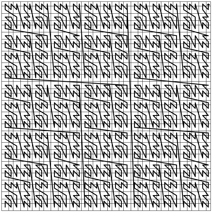
Figure 12: 7th approximant of $F$

3 A Space-Filling Curve Generator Algorithm

In this section we generalise the argument presented in Section 2.

Theorem 3.1.

Let ${\mathcal{P}}$ be a given finite collection of tiles in ${\mathbb{R}}^{2}$. Suppose $\omega$ is a substitution defined over ${\mathcal{P}}$ such that $\max\{diam(t):\ t\in\lambda^{-n}\omega^{n}(p),\ p\in{\mathcal{P}}\}\downarrow 0$ as $n\to\infty$, where $diam(t)$ denotes the diameter of ${\mathrm{supp\ }}t$ and $\lambda$ denotes the expansion factor of $\omega$. Then for each $p\in{\mathcal{P}}$ there exists a Cantor set $\Gamma_{\omega,p}\subseteq[0,1]$ and a continuous surjection $f_{\omega,p}:\Gamma_{\omega,p}\mapsto{\mathrm{supp\ }}p$ such that $f_{\omega,p}$ extends to a space-filling curve $F_{\omega,p}:[0,1]\mapsto{\mathrm{supp\ }}p$ by linear interpolation.

Proof.

Let ${\mathcal{P}}$ be a finite collection of tiles. Suppose $\omega:{\mathcal{P}}\mapsto{\mathcal{P}}^{*}$ is a substitution with an expansion factor $\lambda>1$ such that $\max\{diam(t):\ t\in\lambda^{-n}\omega^{n}(q),\ q\in{\mathcal{P}}\}\downarrow 0$ as $n\to\infty$. Assume without loss of generality $|\omega(q)|>1$ for all $q\in{\mathcal{P}}$.

Define a bijection $g_{q}:\omega(q)\mapsto\{1,\dots,|\omega(q)|\}$, for every $q\in{\mathcal{P}}$. For $q\in{\mathcal{P}}$, $g_{q}$ defines a total order $\underset{q,1}{\lesssim}$ between the tiles of $\omega(q)$ such that $x\underset{q,1}{\lesssim}y$ whenever $g_{q}(x)\leq g_{q}(y)$, for $x,y\in\omega(q)$. Extend these total orders to the supertiles of $\omega$ inductively such that

1. If $x,y\in\omega^{n-1}(t)$ for some $t\in\omega(q)$ and $n\in{\mathbb{Z}}^{+}\backslash\{1\}$, then $x\underset{q,n}{\lesssim}y$ whenever $x\underset{q,n-1}{\lesssim}y$.

2. If $x\in\omega^{n-1}(t_{1})$ and $y\in\omega^{n-1}(t_{2})$ for some distinct $t_{1},t_{2}\in\omega(q)$ and $n\in{\mathbb{Z}}^{+}\backslash\{1\}$, then $x\underset{q,n}{\lesssim}y$ whenever $t_{1}\underset{q,1}{\lesssim}t_{2}$.

The total order $\underset{q,n}{\lesssim}$ for $q\in{\mathcal{P}}$ and $n\in{\mathbb{Z}}^{+}$, can be transferred over the scaled patch $\lambda^{-n}\cdot\omega^{n}(q)$. Precisely, for each $q\in{\mathcal{P}}$ and $n\in{\mathbb{Z}}^{+}$, label the scaled tiles in $\lambda^{-n}\cdot\omega^{n}(q)$ by ${\mathcal{J}}^{1}_{q,n},{\mathcal{J}}^{2}_{q,n},\dots,{\mathcal{J}}^{|\omega^{n}(q)|}_{q,n}$ such that ${\mathcal{J}}_{q,n}^{i}\underset{q,n}{\lesssim}{\mathcal{J}}_{q,n}^{j}$ if and only if $i\leq j$. Next we construct a Cantor set.

For each $q\in{\mathcal{P}}$, define a subdivision rule by partitioning a given interval of random length into $2.|w(q)|-1$ many equal length subintervals and removing the even indexed subintervals as shown in Figure 13 and Figure 14, respectively.

Figure 13: $I$ is dissected into $2.|w(q)|-1$ many closed subintervals of length $(2.|w(q)|-1)^{-1}$.

Figure 14: Even number indexed subintervals are removed.

Next, add labels to intervals $I,I_{1},I_{3},\dots,I_{2.|\omega(q)|-1}$ using $g_{q}$ as follows:

$$l(I)=l(q)\quad\mathrm{and}\quad l(I_{2i-1})=l(g_{q}^{-1}(i))\ \mathrm{for\ }i\in\{1,\dots,|\omega(q)|\}.$$

This process defines a subdivision rule of intervals with labels. Let $p\in{\mathcal{P}}$ be fixed. Start with the interval $[0,1]$ with label $l(p)$. Applying the defined subdivision rules inductively induces a Cantor set $\Gamma_{\omega,p}$, as explained in Section 2.4.

Denote the intervals appearing in the n-th step of the construction of $\Gamma_{\omega,p}$ by ${\mathcal{I}}_{p,n}^{1},\dots,{\mathcal{I}}_{p,n}^{|\omega^{n}(p)|}$, from left to right respectively. For each $n\in{\mathbb{Z}}^{+}$, $f_{p,n}:\{{\mathcal{I}}^{k}_{p,n}:\ k=1,\dots,|\omega^{n}(p)|\}\mapsto\{{\mathcal{J}}^{k}_{p,n}:\ k=1,\dots,|\omega^{n}(p)|\}$ defined by $f_{p,n}({\mathcal{I}}^{k}_{p,n})={\mathcal{J}}^{k}_{p,n}$ for $k=1,\dots,|\omega^{n}(p)|$ is a well-defined bijection. For each $x\in\Gamma_{\omega,p}$ and $n\in{\mathbb{N}}$, there exists $k_{p,n}\in\{1,\dots,|\omega^{n}(p)|\}$ such that $x\in{\mathcal{I}}_{p,n}^{k_{p,n}}$. In particular, $\{x\}=\bigcap\limits_{n=1}^{\infty}{\mathcal{I}}_{p,n}^{k_{p,n}}$ by Cantor’s intersection theorem. By the same token, there exists $y\in{\mathrm{supp\ }}p$ such that $\{y\}=\bigcap\limits_{n=1}^{\infty}{\mathcal{J}}_{p,n}^{k_{p,n}}$. This process induces a surjection $f_{\omega,p}:\Gamma_{\omega,p}\mapsto{\mathrm{supp\ }}p$ such that $f_{\omega,p}(x)=y$ where $x$ and $y$ are as defined above. Next we prove that $f_{\omega,p}$ is continuous.

For each $n\in{\mathbb{Z}}^{+}$, define the following:

$$g_{p,n} =\max\limits_{j\in\{1,\dots,|\omega^{n}(p)|\}}\left\{l({\mathcal{I}}^{j}_{p,n}):\ l({\mathcal{I}}^{j}_{p,n})\ \mathrm{denotes\ the\ length\ of\ }{\mathcal{I}}^{j}_{p,n}\right\},$$

$$h_{p,n} =\max\limits_{j\in\{1,\dots,|\omega^{n}(p)|\}}\left\{diam({\mathcal{J}}^{j}_{p,n}):\ diam({\mathcal{J}}^{j}_{p,n})\ \mathrm{denotes\ the\ diameter\ of\ }{\mathcal{J}}^{j}_{p,n}\right\}.$$

We have that $g_{p,n}\downarrow 0$ and $h_{p,n}\downarrow 0$ as $n\to\infty$. Choose $x\in\Gamma_{\omega,p}$ and $\epsilon>0$. Pick $N_{p}\in{\mathbb{Z}}^{+}$ sufficiently large so that $h_{p,N_{p}}<\epsilon$. Set $\delta=\frac{g_{p,N_{p}}}{2}$. If $y\in\Gamma_{\omega,p}$ with $|x-y|<\delta$ then $x,y\in{\mathcal{I}}_{p,N_{p}}^{j_{0}}$ for some $j_{0}\in\{1,\dots,|\omega^{N_{p}}(p)|\}$. That is, $f(x),f(y)\in{\mathcal{J}}_{p,N_{p}}^{j_{0}}$ and $||f(x)-f(y)||<\epsilon$. Thus, $f_{\omega,p}$ is continuous, and extends to a space-filling curve $F_{\omega,p}:[0,1]\mapsto{\mathrm{supp\ }}p$ by linear interpolation. ∎

Theorem 3.1 can be regarded as an algorithm. Precisely, for every finite substitution $\omega:{\mathcal{P}}\mapsto{\mathcal{P}}^{*}$ satisfying the condition in Theorem 3.1, and a tile $p\in{\mathcal{P}}$, the following steps form a space-filling curve.

$\mathbf{Step-1:}$ Choose $k\in{\mathbb{Z}}^{+}$ such that $|\omega^{k}(q)|>1$ for every $q\in{\mathcal{P}}$.

Remark 3.2.

Replace $\omega$ with $\omega^{k}$ for the following steps. We assume without loss of generality $k=1$ for the following steps.

$\mathbf{Step-2:}$ Define a bijection $g_{q}:\omega(q)\mapsto\{1,\dots,|\omega(q)|\}$, for all $q\in{\mathcal{P}}$.

$\mathbf{Step-3:}$ The maps $\{g_{q}:\ q\in{\mathcal{P}}\}$ indicate total orders over the supertiles of $\omega$. Label the scaled tiles in $\lambda^{-n}\cdot\omega^{n}(p)$ for each $p\in{\mathcal{P}}$ and $n\in{\mathbb{Z}}^{+}$, according to the generated total order structures.

$\mathbf{Step-4:}$ Construct a Cantor set $\Gamma_{\omega,p}$.

$\mathbf{Step-5:}$ Define a bijection between the intervals appearing in the n-th construction step of $\Gamma_{\omega,p}$ and the scaled tiles in the collection $\lambda^{-n}\cdot\omega^{n}(p)$, for each $n\in{\mathbb{Z}}^{+}$.

$\mathbf{Step-6:}$ Construct a continuous surjection $f_{\omega,p}:\Gamma_{\omega,p}\mapsto{\mathrm{supp\ }}p$ using the bijective correspondences described in Step - 5.

$\mathbf{Step-7:}$ Construct a space-filling curve $F_{\omega,p}:[0,1]\mapsto{\mathrm{supp\ }}p$ by linear interpolation over $f_{\omega,p}$.

3.1 Space-Filling Curve Examples

In Section 3.1 we apply the algorithm induced from Theorem 3.1 using some of the known substitutions. The substitutions provided in this section, as well as a vast collection of other substitutions, can be found at [1]. The generated space-filling curves are elucidated by their associated approximants (Definition 3.3).

Definition 3.3.

Let $F_{\omega,p}$ be a space filling curve constructed by the algorithm in Section 3. With the same notations in the proof of Theorem 3.1, for each $n\in{\mathbb{Z}}^{+}$ and $j\in\{1,\dots,|\omega^{n}(p)|\}$, denote the centre of ${\mathcal{J}}^{j}_{p,n}$ by $x({\mathcal{J}}^{j}_{p.n})$. The directed curve formed by joining the points $x({\mathcal{J}}^{1}_{p.n}),x({\mathcal{J}}^{2}_{p.n}),\dots,x({\mathcal{J}}^{|\omega^{n}(p)|}_{p.n})$ successively is called the n-th approximant of $F_{\omega,p}$.

Example 3.4 (Thue-Morse).

Consider the substitution given in Figure 15. The substitution is called 2-dimensional Thue-Morse substitution (2DTM in short). It is defined over two unit squares with labels $A,B$. The expansion factor for this substitution is $2$. Choose a square tile with label $A$ to input in the algorithm. Define an order structure over the 1-supertiles of 2DTM through the curves depicted in Figure 16, according to which tile is visited first by the curves. The associated orders are described by the numbers attached to the tiles in Figure 17. Then the space-filling curve generated by the algorithm is nothing but the Lebesgue curve.

On the other hand, define another order structure over the 1-supertiles of 2DTM by the curves shown in Figure 18. Let $F_{tm}^{A}$ denote the space-filling curve formed by the algorithm (by inputting a tile with label $A$). First four approximants of $F_{tm}^{A}$ are shown in Figure 19.

Figure 15: 2-dimensional Thue-Morse substitution

Figure 16: Total orders defined through curves for the 1-supertiles of 2DTM

Figure 17: Total orders over 1-supertiles of 2DTM

Figure 18: Total orders over 1-supertiles of 2DTM

Figure 19: First four approximants of $F_{tm}^{A}$

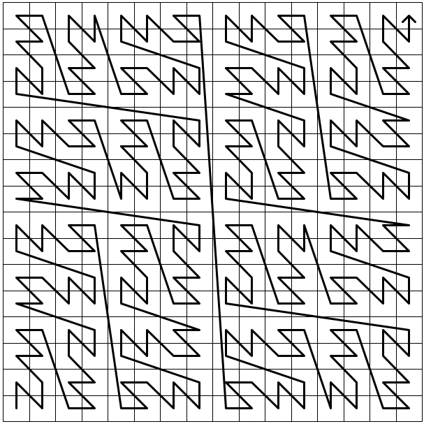
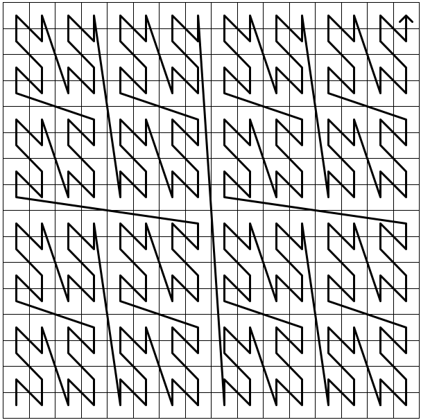
Figure 20: 4th approximants of $F_{tm}^{A}$ and the Lebesgue curve, respectively

Example 3.5 (Equithirds-variant).

Consider the substitution depicted in Figure 21. The substitution is a variation of Equithirds substitution [1]. It is defined over four tiles and their rotations, which are constructed by two different shapes, an equilateral triangle with side length $1$ and an isosceles triangle with side lengths $1,1,\sqrt{3}$. Its expansion factor is $\sqrt{3}$. The curves shown in Figure 22 describe total orders over its 1-supertiles. Let $F^{i}_{eq}$ denote the space-filling curve produced by the algorithm from the tile with label $i$ for $i\in\{A^{+},A^{-},B^{+},B^{-}\}$. First four approximants of $F^{A^{+}}_{eq}$ are shown in Figure 23 and first four approximants of $F^{B^{+}}_{eq}$ are shown in Figure 24. Observe that $F^{B^{+}}_{eq}(0)=F^{B^{+}}_{eq}(1)$. So, for illustration purposes, we modify the approximants of $F^{B^{+}}_{eq}$ to be closed curves. We connect the end points of its approximant curves with a straight line and fill the associated closed regions as demonstrated in Figure 25 and Figure 26.

Figure 21: Equithirds-variant

Figure 22: Total orders over the 1-supertiles of Equithirds-variant

Figure 23: First four approximants of $F^{A^{+}}_{eq}$

Figure 24: First four approximants of $F^{B^{+}}_{eq}$

Figure 25: 1st, 3rd, 5th and 7th approximants of $F^{B^{+}}_{eq}$ where the end points of the approximants are joined with a line and the associated closed regions are filled. The 7th approximant is scaled up for illustration purposes.

Figure 26: 2nd, 4th, 6th and 8th approximants of $F^{B^{+}}_{eq}$ where the end points of the approximants are joined with a line and the associated closed regions are filled. The 8th approximant is scaled up for illustration purposes.

Next we describe the geometry of approximants of $F^{A^{+}}_{eq}$. Notice that $F^{A^{+}}_{eq}(0)\neq F^{A^{+}}_{eq}(1)$. Let $p_{A^{+}}^{r}$ denote the rotated version of $p_{A^{+}}$ by $\pi$ such that their longer edges merge. Also, denote the space filling curves generated by these two tiles by $F^{A^{+}}_{eq},F^{A^{+}_{r}}_{eq}$. Since $F^{A^{+}}_{eq}(0)=F^{A^{+}_{r}}_{eq}(1)$ and $F^{A^{+}}_{eq}(1)=F^{A^{+}_{r}}_{eq}(0)$, we can concatenate $F^{A^{+}}_{eq}$ with $F^{A^{+}_{r}}_{eq}$ in order to define another space-filling curve $F^{A}_{eq}$ so that $F^{A}_{eq}(0)=F^{A}_{eq}(1)$. The geometry of approximants of $F^{A^{+}}_{eq}$ will be visualised through approximants of $F^{A}_{eq}$ since we can modify the approximants of $F^{A}_{eq}$ to be closed curves as shown in Figure 27. The associated filled regions of the first 8 approximant curves are shown in Figure 28 and Figure 29.

Figure 27: First four approximants of $F^{A}_{eq}$ where their end points are joined with a line.

Figure 28: Filled versions of 1st, 3rd, 5th and 7th approximants of $F^{A}_{eq}$. The 7th approximant is scaled up for demonstration purposes.

Figure 29: Filled versions of 2nd, 4th, 6th and 8th approximants of $F^{A}_{eq}$. The 8th approximant is scaled up for demonstration purposes.

For the following two substitution examples, we will use the algorithm (Theorem 3.1) to create space filling curves over patches instead of tiles, similar to the construction of $F_{eq}^{A}$, for demonstration purposes.

Example 3.6 (Pinwheel-variant).

The substitution in Figure 30 is defined over four tiles and their rotations. It is a variation of Pinwheel substitution [1]. Every tile in the substitution is a right triangle with side lengths $1,2,\sqrt{5}$. The expansion factor for this substitution is $\sqrt{5}$. The curves in Figure 31 define total orders over 1-supertiles of this substitution. Let $R_{1},R_{2}$ denote the regions, rhombus and rectangle, shown in Figure 32. Using the algorithm together with the defined total orders, we can produce two space-filling curves $F_{pin}^{1},F_{pin}^{2}$ over $R_{1},R_{2}$, respectively. Figure 33 indicates the first two approximants of $F_{pin}^{1}$ and $F_{pin}^{2}$. Observe that $F^{i}_{pin}(0)=F^{i}_{pin}(1)$ for $i=1,2$.

Figure 34 and Figure 35 demonstrates the first 5 approximants of $F_{pin}^{1}$, whereas Figure 36 and Figure 37 illustrates the first 6 approximants of $F_{pin}^{2}$.

Figure 30: Pinwheel-variant substitution

Figure 31: Total orders over 1-supertiles of the Pinwheel-variant substitution

Figure 32: The regions $R_{1}$ and $R_{2}$, from left to right respectively

Figure 33: First two approximants of $F^{1}_{pin}$ and $F^{2}_{pin}$

Figure 34: 1st, 3rd and 5th approximants of $F^{1}_{pin}$ - filled version. The 5th approximant is scaled up for illustration purposes.

Figure 35: 2nd and 4th approximants of $F^{1}_{pin}$ - filled version.

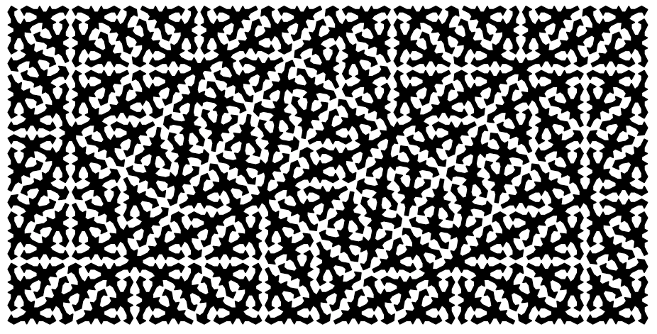
Figure 36: 1st, 3rd and 5th approximants of $F^{2}_{pin}$ - filled version. The 5th approximant is scaled up for illustration purposes.

Figure 37: 2nd, 4th and 6th approximants of $F^{2}_{pin}$ - filled version. The 6th approximant is scaled up for illustration purposes.

Example 3.7 (Penrose-Robinson-variant).

Start with the substitution given in Figure 38. Its domain consists of $12$ tiles and their rotations, which are congruent copy of two different shapes, an isosceles triangle with side lengths $1,1,(1+\sqrt{5})/2$ and an isosceles triangle with side lengths $1,1,(\sqrt{5}-1)/2$. The expansion factor for this substitution is the golden mean $(1+\sqrt{5})/2$. It is a variation of Penrose-Robinson substitution [1]. Define the total orders described in Figure 39. Using the described total orders we generate space filling curves $F_{star},F_{deca}$ that fill the supports of the patches shown in Figure 40, respectively, such that $F_{star}(0)=F_{star}(1)$ and $F_{deca}(0)=F_{deca}(1)$. The associated approximants of $F_{star}$ and $F_{deca}$ are shown in Figure 41, Figure 42 and Figure 43.

Figure 38: Penrose-Robinson-variant substitution. 1-supertiles are scaled down for demonstration.

Figure 39: Total orders over 1-supertiles of the Penrose-Robinson-variant substitution

Figure 40: A star and a decagon.

Figure 41: First four approximants of $F_{star}$ - filled version

Figure 42: First four approximants of $F_{deca}$ - filled version

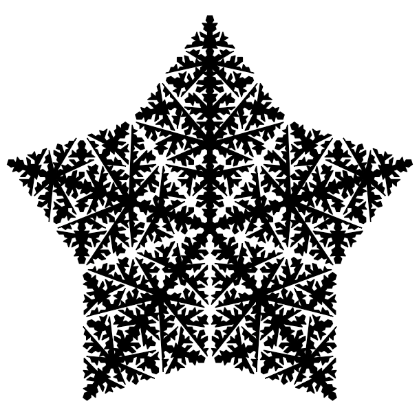
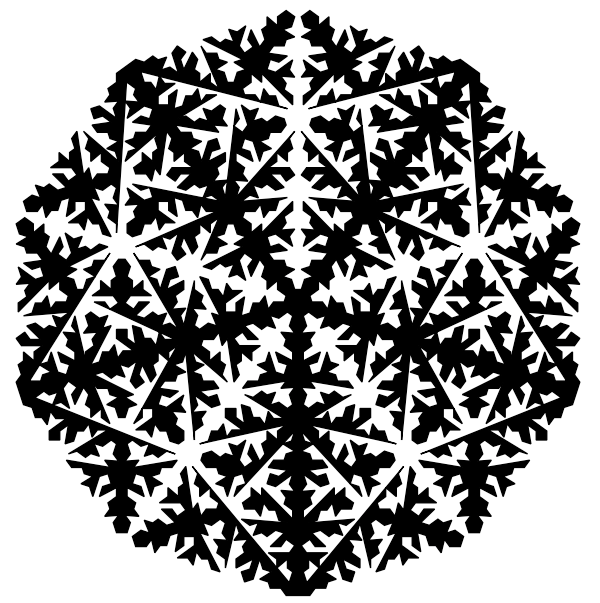
Figure 43: 6th approximants of $F_{star}$ and $F_{deca}$, from left to right.

4 Substitutions to Fractal-like Relatively Dense Sets

Definition 4.1.

A substitution $\omega:{\mathcal{P}}\mapsto{\mathcal{P}}^{*}$ is called primitive if there exists $k\in{\mathbb{Z}}^{+}$ such that $\omega^{k}(p)$ contains a copy of $q$ for every $p,q\in{\mathcal{P}}$.

Primitive substitutions induce coverings of the plane, called tilings, with tiles sharing at most their boundaries. The details of such construction can be found in [5, Theorem 1.4] or [4, P:12-13]. We inherit the same idea to produce fractal-like relatively dense sets in the plane.

Proposition 4.2.

Let $\omega:{\mathcal{P}}\mapsto{\mathcal{P}}^{*}$ be a given substitution defined over a finite collection ${\mathcal{P}}$ with an expansion factor $\lambda>1$ such that $\max\{diam(t):\ t\in\lambda^{-n}\omega^{n}(p),\ p\in{\mathcal{P}}\}\downarrow 0$ as $n\to\infty$, where $diam(t)$ denotes the diameter of ${\mathrm{supp\ }}t$. Suppose $F:[0,1]\mapsto{\mathrm{supp\ }}p$ is a Lebesgue-type space filling curve generated by the method explained in Theorem 3.1 and fills ${\mathrm{supp\ }}p$ for some $p\in{\mathcal{P}}$. Assume that $F(0)=F(1)$ and $\{F_{n}:\ n\in{\mathbb{Z}}^{+}\}$ is the collection of approximants of $F$ $($defined on $\lambda^{-n}\omega^{n}(p))$ generated by filling the associated closed regions $($i.e. $F_{n}$’s are sets in ${\mathbb{R}}^{2})$. Assume further there exists $x\in{\mathbb{R}}^{2}$ and $k\in{\mathbb{Z}}^{+}$ so that

1. $p+x\in\omega^{n}(p+x)$,

2. ${\mathrm{supp\ }}(p+x)\cap{\partial\mathrm{supp\ }}\omega^{n}(p+x)=\emptyset$,

3. $F_{1}+x\subseteq\lambda^{n}(F_{n+1}+x)$,

4. $F_{n}$ visits two $($scaled$)$ tiles in $\lambda^{-n}\omega^{n}(p)$ subsequently only if they share a common edge, for every $n\in{\mathbb{Z}}^{+}$.

Then

• $F_{k.n+1}+x\subseteq\lambda^{n}(F_{(k+1)n+1}+x)$ for every $k\in{\mathbb{Z}}^{+}$. In particular,

  $$F_{1}+x\subseteq\lambda^{n}(F_{n+1}+x)\subseteq\lambda^{2n}(F_{2n+1}+x)\subseteq\lambda^{3n}(F_{3n+1}+x)\subseteq\dots$$

• $F=\bigcup\limits_{i=0}^{\infty}\lambda^{in}(F_{in+1}+x)$ is a relatively dense set in the plane.

• There exists a collection of sets $\{A_{k}:k\in{\mathbb{Z}}^{+}\}$ so that

  • $\bigcup\limits_{k}A_{k}=F$,

  • $int(A_{i})\cap int(A_{j})=\emptyset$ whenever $i\neq j$, where $int(A_{i}),int(A_{j})$ are interiors of $A_{i}$ and $A_{j}$,respectively,

  • There are finite number of indices $k_{1},\dots k_{m}\in{\mathbb{Z}}^{+}$ for some $m\in{\mathbb{Z}}^{+}$ such that for each $k\in{\mathbb{Z}}^{+}$ there exists $n_{k}\in\{k_{1},\dots,k_{m}\}$ and $x_{k}\in{\mathbb{R}}^{2}$ with $A_{k}=A_{n_{k}}+x_{k}$.

Proof.

• We get $\{p+x\}\subseteq\omega^{n}(p+x)\subseteq\omega^{2n}(p+x)\subseteq\dots$, by $(1)$. So, we can conclude by $(3)$ that

  $$F_{1}+x\subseteq\lambda^{n}(F_{n+1}+x)\subseteq\lambda^{2n}(F_{2n+1}+x)\subseteq\lambda^{3n}(F_{3n+1}+x)\subseteq\dots.$$

• We have that the collection $T=\bigcup\limits_{i=1}\omega^{in}(p+x)$ is a covering of the plane by $(1)$ and $(2)$ [4, P:12-13]. Note that $F=\bigcup\limits_{i=0}^{\infty}\lambda^{in}(F_{in+1}+x)$ visits every tile in $T$. Thus, $F$ is relatively dense in ${\mathbb{R}}^{2}$ because there are only finitely many tiles in ${\mathcal{P}}$.

• For each $t\in T$, define $A_{t}=F\cap{\mathrm{supp\ }}t$. Then $F=\bigcup\limits_{t\in T}A_{t}$. Furthermore, $int(A_{t_{i}})\cap int(A_{t_{j}})=\emptyset$ whenever $t_{i}\neq t_{j}$, where $int(A_{t_{i}}),int(A_{t_{j}})$ are interiors of $A_{t_{i}},A_{t_{j}}$, respectively. By $(4)$ and the fact that $|{\mathcal{P}}|$ is finite, there are only finitely many indices $t_{1},\dots,t_{m}$ for some $m\in{\mathbb{Z}}^{+}$ such that for each $t\in T$, there exists $s_{t}\in\{t_{1},\dots,t_{m}\}$ and $x_{t}\in{\mathbb{R}}^{2}$ with $A_{t}=A_{s_{t}}+x_{t}$. ∎

Remark 4.3.

The condition $c$ in the proposition is akin to the definition of fractals by Mandelbrot [3]. In particular, condition $c$ assures that there are finite number dissections of $F$, whose collection is denoted as ${\mathcal{P}}$ (analogue to tile set ${\mathcal{P}}$), such that $F$ can be written as a countable union of sets, each of which is a translational copy of the defined dissections of $F$ (i.e. each of which is a congruent copy of a tile in ${\mathcal{P}}$).

An Example (Equithirds):

Consider the substitution $\omega_{eq}$ given in Figure 21. Let $p$ denote the prototile with label $B^{+}$. Observe that there exists $x\in{\mathbb{R}}^{2}$ such that $p_{B^{+}}+x\in\omega_{eq}^{4}(p_{B^{+}}+x)$ and ${\mathrm{supp\ }}p_{B^{+}}+x\cap{\partial\mathrm{supp\ }}\omega_{eq}^{4}(p_{B^{+}}+x)=\emptyset$. Let $\{F_{eq,k}^{B^{+}}:\ k\in{\mathbb{Z}}^{+}\}$ denote the set of approximants of $F_{eq}^{B^{+}}$, first 8 of which are depicted in Figure 25 and Figure 26. Note also that

$${\displaystyle F_{eq,1}^{B^{+}}+x\subseteq\sqrt{3}^{4}F_{eq,4}^{B^{+}}+x,}$$

as demonstrated in Figure 44. Hence,

$${\displaystyle F=\bigcup\limits_{i=0}^{\infty}\sqrt{3}^{4i}F_{eq,4i+1}^{B^{+}}+x}$$

is a relatively dense fractal-like set in the plane, by Proposition 4.2.

Figure 44:

Acknowledgements. This work was supported by the Ministry of National Education of Turkey.

Data Availability Statement. Data sharing not applicable to this article as no datasets were generated or analysed during the current study.

The Roslin Institute, The University of Edinburgh, Easter Bush Campus, EH25 9RG, Edinburgh, United Kingdom

E-mail address: iozkarac@ed.ac.uk

References

- [1] Frettlöh D., Harriss E., Gähler F.: Tilings encyclopedia, https://tilings.math.uni-bielefeld.de/
- [2] Lebesgue, H.: Leçons sur l’Intégration et la Recherche des Fonctions Primitives, 44-45. Gauthier-Villars, Paris (1904)
- [3] Mandelbrot, B.B., The Fractal Geometry of Nature, Macmillan (1983)
- [4] Ozkaraca, M.I., An application of space filling curves to substitution tilings, Doctoral dissertation, University of Glasgow (2021).
- [5] Sadun, L., Topology of Tiling Spaces, American Mathematical Society (2008)
- [6] Sagan, H.: Approximating Polygons for Lebesgue’s and Schoenberg’s Space-Filling Curves, American Mathematical Monthly, (5), 361-368 (1986)
- [7] Sagan, H.: A Geometrization of Lebesgue’s Space-filling Curve, Mathematical Intelligencer, (4), 37-43 (1993)
- [8] Sagan, H., Space-Filling Curves, Springer-Verlag, Berlin Heidelberg New York, (1994)
- [9] Wunderlich, W.: Über Peano-Kurven, Elemente der Mathematik, , 1-10 (1973)