Visual Attention Emerges from Recurrent Sparse Reconstruction

Abstract

Visual attention helps achieve robust perception under noise, corruption, and distribution shifts in human vision, which are areas where modern neural networks still fall short. We present VARS, Visual Attention from Recurrent Sparse reconstruction, a new attention formulation built on two prominent features of the human visual attention mechanism: recurrency and sparsity. Related features are grouped together via recurrent connections between neurons, with salient objects emerging via sparse regularization. VARS adopts an attractor network with recurrent connections that converges toward a stable pattern over time. Network layers are represented as ordinary differential equations (ODEs), formulating attention as a recurrent attractor network that equivalently optimizes the sparse reconstruction of input using a dictionary of “templates” encoding underlying patterns of data. We show that self-attention is a special case of VARS with a single-step optimization and no sparsity constraint. VARS can be readily used as a replacement for self-attention in popular vision transformers, consistently improving their robustness across various benchmarks. Code is released on GitHub (https://github.com/bfshi/VARS).

1 Introduction

One of the hallmarks of human visual perception is its robustness under severe noise, corruption, and distribution shifts (Biederman, 1987; Bisanz et al., 2012). Although having surpassed human performance on ImageNet (He et al., 2015), convolutional neural networks (CNNs) are still far behind the human visual systems on robustness (Dodge & Karam, 2017; Geirhos et al., 2017) – CNNs are vulnerable under random image corruption (Hendrycks & Dietterich, 2019), adversarial perturbation (Szegedy et al., 2013), and distribution shifts (Wang et al., 2019; Djolonga et al., 2021).

Vision transformers (Dosovitskiy et al., 2020) have been reported to be more robust to image corruption and distribution shifts than CNNs under certain conditions (Naseer et al., 2021; Paul & Chen, 2021). One hypothesis is that the self-attention module, a key component of vision transformers, helps improve robustness (Paul & Chen, 2021), achieving state-of-the-art performance on a variety of robustness benchmarks (Mao et al., 2021). Although the robustness of vision transformers still seems to be far behind human vision (Hendrycks et al., 2021a; Dodge & Karam, 2017), recent work suggests that attention is a key to achieving (perhaps human-level) robustness in computer vision.

The cognitive science literature has also suggested a close relationship between attention mechanisms and robustness in human vision (Kar et al., 2019; Wyatte et al., 2012). For example, visual attention in human vision has been shown to selectively amplify certain patterns in the input signal and repress others that are not desired or meaningful, leading to robust recognition under challenging conditions such as occlusion (Tang et al., 2018), clutter (Mnih et al., 2014; Walther et al., 2005), and severe corruptions (Wyatte et al., 2014). These findings motivate us to improve robustness of neural networks by designing attention inspired by the human visual attention. However, despite the existing computational models of human visual attention (e.g., Li (2014)), their concrete instantiation in DNNs is still missing, and the connection between human visual attention and existing attention designs is also vague (Sood et al., 2020).

In this work, we introduce VARS—Visual Attention from Recurrent Sparse reconstruction—a new attention formulation inspired by the recurrency and sparsity commonly observed in the human visual system. Human visual attention contains the process of grouping and selecting salient features while repressing irrelevant signals (Desimone & Duncan, 1995). One of its neural foundations is the recurrent connections between neurons in the same layer, as opposed to the feed-forward connections from lower to higher layers (Stettler et al., 2002; Gilbert & Wiesel, 1989; Bosking et al., 1997; Li, 1998; Lamme & Roelfsema, 2000). By iteratively connecting neurons, salient features with strong correlations are grouped and amplified (Roelfsema, 2006; O’Reilly et al., 2013). Sparsity, on the other hand, also plays an important role in visual attention, where distracting information is muted by the sparsity constraint and only the most salient parts of the input remains (Chaney et al., 2014; Wright et al., 2008). Sparsity is also a natural outcome of recurrent connections (Rozell et al., 2008), and the two together can be used to formulate visual attention.

Built upon this observation, VARS shows that visual attention naturally emerges from a recurrent sparse reconstruction of input signals in deep neural networks. We start from an ordinary differential equation (ODE) description of neural networks and adopt an attractor network (Grossberg & Mingolla, 1987; Zucker et al., 1989; Yen & Finkel, 1998) to describe the recurrently connected neurons that arrive at an equilibrium state over time. We then reformulate the computation model into an encoder-decoder style module and show that by adding inhibitory recurrent connections between the encoding neurons, the ODE is equivalent to optimizing the sparse reconstruction of the input using a learned dictionary of “templates” encoding underlying data patterns. In practice, the feed-forward pathway of our attention module only involves optimizing the sparse reconstruction, which can be efficiently solved by the iterative shrinkage-thresholding algorithm (Beck & Teboulle, 2009).

We present multiple variants of VARS by instantiating the learned dictionary in the sparse reconstruction as a static (input-independent), dynamic (input-dependent), or static+dynamic (combination of the two) set of templates. We show that the existing self-attention design (Vaswani et al., 2017), widely adopted in vision transformers, is a special case of VARS with a dynamic dictionary but only using a single step update of the ODE without sparsity constraints. VARS extends self-attention and exhibits higher robustness in practice.

We evaluate VARS on five large-scale robustness benchmarks of naturally corrupted, adversarially perturbed and out-of-distribution images on ImageNet, where VARS consistently outperforms previous methods. We also assess the quality of attention maps on human eye fixation and image segmentation datasets, and show that VARS produces higher quality attention maps than self-attention.

2 Related Work

Recurrency in vision. Recurrent connections are as ubiquitous as feed-forward connections in the human visual system (Felleman & Van Essen, 1991). Various phenomena in human vision are credited to recurrency, such as visual grouping and pattern completion (Roelfsema et al., 2002; O’Reilly et al., 2013), robust recognition and segmentation under clutter (Vecera & Farah, 1997), and even perceptual illusions (Mély et al., 2018).

In deep learning, Nayebi et al. (2018) find that convolutional recurrent models can better capture neural dynamics in the primate visual system. Other work has designed recurrent modules to help networks attend to salient features such as contours (Linsley et al., 2020), to group and segregate an object from its context (Kim et al., 2019; Darrell et al., 1990), or to conduct Bayesian inference of corrupted images (Huang et al., 2020).  Zoran et al. (2020) combine an LSTM (Hochreiter & Schmidhuber, 1997) and self-attention to improve adversarial robustness. However, the LSTM is only used to generate the queries of self-attention and does not affect the attention mechanism itself. Instead, we show visual attention emerges from recurrency and can be formulated as a recurrent contractor network, which is equivalent to optimizing sparse reconstruction of the input signals.

Sparsity in vision. It has long been hypothesized that the primary visual cortex (V1) encodes incoming stimuli in a sparse manner (Olshausen & Field, 1997). Olshausen & Field (1996) show that localized and oriented filters resembling the simple cells in the visual cortex can spontaneously emerge through dictionary learning via sparse coding. Some work has extended this hypothesis to the prestriate cortex such as V2 (Lee et al., 2007).  Rozell et al. (2008) propose Locally Competitive Algorithms (LCA) as a biologically-plausible neural mechanism for computing sparse representations in the visual cortex based on neural recurrency.

Recently there are studies on designing sparse neural networks, but they mostly focus on reducing the computational complexity via sparse weights or connections (Hoefler et al., 2021; Liu et al., 2019; Guo et al., 2018). Other work has exploited sparse data structure in neural networks  (Wu et al., 2019; Fan et al., 2020). In this work, we draw a connection between sparsity and recurrency as well as visual attention and build a new attention formulation on top of it to improve the robustness of deep neural networks.

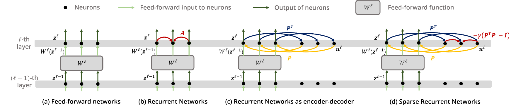
Figure 1: Illustrations on neural dynamics. (a) Feed-forward networks. The output $\mathbf{z}^{\ell-1}$ from the $(\ell-1)$-th layer’s neurons is processed by the feed-forward function $W^{\ell}$ into $W^{\ell}(\mathbf{z}^{\ell-1})$, used as the input to the $\ell$-th layer’s neurons. The $\ell$-th layer’s neuron output $\mathbf{z}^{\ell}$ is identical to the input. (b) Recurrent networks. When the $\ell$-th layer’s neurons are recurrently connected, the output $\mathbf{z}^{\ell}$ is wired back by weight matrix $\mathbf{A}$ serving as an additional input to the neurons. The final output is the steady state $\mathbf{z}^{\ell^{\ast}}=\mathbf{A}\mathbf{z}^{\ell^{\ast}}+W^{\ell}(\mathbf{z}^{\ell-1})$. (c) Recurrent networks as encoder-decoder. The neurons with recurrent connections in (b) have the same steady state as an encoder-decoder structure, where the auxiliary layer encodes $\mathbf{z}^{\ell}$ by $\mathbf{P}^{T}$ and its output is decoded by $\mathbf{P}$ and sent back. (d) Sparse recurrent networks. We adopt a sparse structure in the encoding by adding inhibitive recurrent connections $-\gamma(\mathbf{P}^{T}\mathbf{P}-\mathbf{I})$ between $\mathbf{u}^{\ell}$.

Visual attention and robustness. Attention widely exists in human brains (Scholl, 2001) and is adopted in machine learning models (Vaswani et al., 2017). A number of studies focus on object-based and bottom-up attention. Various computational models have been proposed for visual attention (Koch & Ullman, 1987; Itti & Koch, 2001; Li, 2014), where neural recurrency help highlight salient features.

In deep learning, the attention mechanism is widely used to process language or visual data (Vaswani et al., 2017; Dosovitskiy et al., 2020). The recently proposed self-attention based vision transformers (Dosovitskiy et al., 2020) can scale to large datasets better than conventional CNNs and achieve better robustness under distribution shifts (Mao et al., 2021; Naseer et al., 2021; Paul & Chen, 2021).

In a complementary line of work to address model robustness, researchers have shown that model robustness can be improved through data augmentation (Geirhos et al., 2018; Rebuffi et al., 2021), designing more robust model architectures (Dong et al., 2020) and training strategies (Madry et al., 2017; Wang et al., 2021b). Some other work (Machiraju et al., 2021; Shi et al., 2020) improves model robustness from a bio-inspired view. In this work, we propose a new attention design, (partially) inspired by human vision systems, which can be used as a replacement for self-attention in vision transformers to further improve model robustness.

3 VARS Formulation

In this section, we first formulate the neural recurrency based on an ODE description of neural dynamics (Section 3.1) and show its equivalence to optimizing the sparse reconstruction of the inputs (Section 3.2). Then we draw a connection between visual attention and recurrent sparse reconstruction and describe the design of VARS (Section 3.3). We find self-attention is a special case of VARS (Section 3.4) and give different model instantiations in Section 3.5.

3.1 Neural Recurrency

ODE descriptions of neural dynamics. We start with an ODE description of feed-forward neural networks (Dayan & Abbott, 2001). Let $\mathbf{z}^{\ell}\in\mathbb{R}^{d}$ denote the output of the $\ell$-th layer’s neurons in a neural network. In a feed-forward neural network, the output of the $\ell$-th layer is

$$\small\mathbf{z}^{\ell}=W^{\ell}(\mathbf{z}^{\ell-1}),$$ (1)

where $W^{\ell}(\cdot)$ is a feed-forward function (e.g., a convolutional or fully connected operator). This equation can be viewed as an equilibrium state ($\derivative{\mathbf{z}^{\ell}}{t}=0$) of the following differential equation:

$$\small\derivative{\mathbf{z}^{\ell}}{t}=-\mathbf{z}^{\ell}+W^{\ell}(\mathbf{z}^{\ell-1}),$$ (2)

which defines the neural dynamics of $\ell$-th layer’s neurons. This can be seen as the (simplified) dynamics of biological neurons: $\mathbf{z}^{\ell}$ is the membrane potential which is charged by the feed-forward input $W^{\ell}(\mathbf{z}^{\ell-1})$ and discharged by the self leakage $-\mathbf{z}^{\ell}$ (Dayan & Abbott, 2001). Note that in the feed-forward case, the output $\mathbf{z}^{\ell}$ of the neurons is identical to the input $W^{\ell}(\mathbf{z}^{\ell-1})$. Figure 1(a) provides an illustration.

Horizontal recurrent connections. In the feed-forward case, the input $W^{\ell}(\mathbf{z}^{\ell-1})$ to the $\ell$-th layer solely depends on the output $\mathbf{z}^{\ell-1}$ from the previous layer. However, when the neurons in the $\ell$-th layer are recurrently connected (illustrated in Figure 1(b)), the input also depends on the $\ell$-th layer’s output $\mathbf{z}^{\ell}$ itself, which we denote by $\widetilde{W}^{\ell}(\mathbf{z}^{\ell-1},\mathbf{z}^{\ell})$. Therefore, the output of a recurrently connected layer is the equilibrium state of an updated differential equation

$$\small\derivative{\mathbf{z}^{\ell}}{t}=-\mathbf{z}^{\ell}+\widetilde{W}^{\ell}(\mathbf{z}^{\ell-1},\mathbf{z}^{\ell}).$$ (3)

In this case, the equilibrium $\mathbf{z}^{\ell^{\ast}}=\widetilde{W}^{\ell}(\mathbf{z}^{\ell-1},\mathbf{z}^{\ell^{\ast}})$ typically does not have a closed-form solution, and in practice the differential equation is often solved by rolling out each step of updates as in recurrent neural networks (RNNs) (e.g., Hochreiter & Schmidhuber (1997)) or by using root-finding techniques (Bai et al., 2019).

Following the previous work by Li (2014), we decompose $\widetilde{W}^{\ell}(\mathbf{z}^{\ell-1},\mathbf{z}^{\ell})$ into a feed-forward input $W^{\ell}(\mathbf{z}^{\ell-1})$ and an additional recurrent input $\mathbf{A}^{\ell}\mathbf{z}^{\ell}$ and rewrite Equation 3 as

$$\small\derivative{\mathbf{z}^{\ell}}{t}=-\mathbf{z}^{\ell}+\mathbf{A}^{\ell}\mathbf{z}^{\ell}+\mathbf{x}^{\ell}$$ (4)

where $\mathbf{x}^{\ell}=W^{\ell}(\mathbf{z}^{\ell-1})$ is the feed-forward input of the neurons in the $\ell$-th layer and $\mathbf{A}^{\ell}\in\mathbb{R}^{d\times d}$, often assumed symmetric and positive semi-definite (Hopfield, 1984; Cohen & Grossberg, 1983), is the weight of horizontal recurrent connections of neurons in the $\ell$-th layer (Figure 1(b)). Note that Equation 4 is also a special case of the continuous attractor neural network (Wu et al., 2016), which is used as a computational model for various neural behaviors such as visual attention (Li, 2014). In what follows, for simplicity and without loss of generality, we only focus on a single-layer scenario and omit the superscript $\ell$.

3.2 Recurrency Entails Sparse Reconstruction

We have defined the neural recurrency in ODEs and now we build its connection to the optimization of sparse reconstruction to understand the functionality of recurrency.

We notice that Equation 4 can also be viewed as an encoder-decoder structure. Since $\{\mathbf{A}\ |\ \mathbf{A}\in\mathcal{S}^{d}_{+}\}=\{\mathbf{P}\mathbf{P}^{T}\ |\ \mathbf{P}\in\mathbb{R}^{d\times d^{\prime}},d^{\prime}\geq d\}$, we can reparameterize $\mathbf{A}$ as $\mathbf{P}\mathbf{P}^{T}$, and turn Equation 4 into

$$\small\derivative{\mathbf{z}}{t}=-\mathbf{z}+\mathbf{P}\mathbf{P}^{T}\mathbf{z}+\mathbf{x},$$ (5)

which has the same steady state solution as

$$\derivative{\mathbf{z}}{t}=-\mathbf{z}+\mathbf{P}\mathbf{u}+\mathbf{x},$$ (6)

$$\derivative{\mathbf{u}}{t}=-\mathbf{u}+\mathbf{P}^{T}\mathbf{z}.$$ (7)

Here, we introduce an auxiliary layer $\mathbf{u}\in\mathbb{R}^{d^{\prime}}$ that receives input $\mathbf{P}^{T}\mathbf{z}$ and converges to $\mathbf{u}^{\ast}=\mathbf{P}^{T}\mathbf{z}^{\ast}$. Meanwhile $\mathbf{z}$ converges to $\mathbf{z}^{\ast}=\mathbf{P}\mathbf{u}^{\ast}+\mathbf{x}$. We can view the steady state solution as an equilibrium between an encoder and a decoder, where the column vectors of $\mathbf{P}$ serve as atoms (or “templates”) of a dictionary, $\mathbf{u}^{\ast}$ is the encoding of $\mathbf{z}^{\ast}$ through the template matching $\mathbf{P}^{T}\mathbf{z}^{\ast}$, and $\mathbf{z}^{\ast}=\mathbf{P}\mathbf{u}^{\ast}+\mathbf{x}$ is the decoding of $\mathbf{u}^{\ast}$ plus a residual connection $\mathbf{x}$. (Figure 1(c)).

Next, we show that this encoder-decoder structure naturally connects with the hypothesis of sparse coding in V1, which states that the encoding of visual signals should be sparse (Olshausen & Field, 1997). Moreover, sparsity naturally emerges as we build the inhibitive recurrent connections between the encoding neurons ($\mathbf{u}$ in our case) (Rozell et al., 2008). To show this, we follow Rozell et al. (2008) and add recurrent connections between $\mathbf{u}$, modeled by the weight matrix $-\gamma(\mathbf{P}^{T}\mathbf{P}-\mathbf{I})$. In addition, we add hyperparameters $\alpha$ and $\beta$ to control the strength of self-leakage, and the element-wise activation functions $\mathit{g}(\cdot)$ to gate the output from the neurons (Dayan & Abbott, 2001). As a result, we update the dynamics of $\mathbf{z}$ and $\mathbf{u}$ as (see also Figure 1(d)):

$$\derivative{\mathbf{z}}{t}=-\alpha\mathbf{z}+\mathbf{P}\mathit{g}(\mathbf{u})+\mathbf{x},$$ (8)

$$\derivative{\mathbf{u}}{t}=-\beta\mathbf{u}-\gamma(\mathbf{P}^{T}\mathbf{P}-\mathbf{I})\mathit{g}(\mathbf{u})+\mathbf{P}^{T}\mathbf{z}.$$ (9)

By taking $\alpha=1$ and $\beta=\gamma=2$ and choosing $\mathit{g}$ as an element-wise thresholding function $\mathit{g}(\mathbf{u}_{i})=\mathit{sgn}(\mathbf{u}_{i})\cdot(\lvert\mathbf{u}_{i}\rvert-\frac{\lambda}{2})_{+}$, where $sgn(\cdot)$ is the sign function, $(\cdot)_{+}$ is ReLU, and $\lambda$ controls the sparse constraint (see Appendix for more details), Equation 8-9 have the equilibrium state as

$$\widetilde{\mathbf{u}}^{\ast} =\operatorname*{arg\,min}_{\widetilde{\mathbf{u}}\in\mathbb{R}^{d^{\prime}}}\frac{1}{2}||\mathbf{P}\widetilde{\mathbf{u}}-\mathbf{x}||^{2}_{2}+\lambda||\widetilde{\mathbf{u}}||_{1},$$ (10)

$$\mathbf{z}^{\ast} =\mathbf{P}\widetilde{\mathbf{u}}^{\ast}+\mathbf{x},$$ (11)

where $\widetilde{\mathbf{u}}=\mathit{g}(\mathbf{u})$ is the gated output of the encoding neurons. We can see that by adding the recurrent connections in $\mathbf{u}$ and the activation functions $\mathit{g}(\cdot)$, the output of $\ell$-th layer’s neurons is not only a simple “copy-paste” of the feed-forward input $\mathbf{x}$ (Equation 1) but also with a sparse reconstruction of the input $\mathbf{P}\widetilde{\mathbf{u}}^{\ast}$. This formulation also indicates that solving the dynamics of a sparse recurrent network is equivalent to sparse reconstruction of the input signal.

3.3 VARS: Attention from Sparse Reconstruction

The core design of VARS is based on the observation that visual attention is achieved through (i) grouping different features and different locations into separate objects and (ii) selecting the most salient objects and suppressing distracting or noisy ones (Desimone & Duncan, 1995). Note that the dynamics of sparse encoding $\mathbf{u}$ (Equation 9) contains a similar process, where the features in $\mathbf{z}$ are grouped by each template $\mathbf{P}^{\mu}$ through $(\mathbf{P}^{\mu})^{T}\mathbf{z}$ and fed into the encoding $\mathbf{u}_{\mu}$, meanwhile the recurrent term $-\gamma(\mathbf{P}^{T}\mathbf{P}-\mathbf{I})\mathit{g}(\mathbf{u})$ imposes a sparse structure on $\mathbf{u}$ so that only the $\mathbf{u}_{\mu}$ that encodes the most salient template objects will survive.

Here we introduce VARS, a module that achieves visual attention via sparse reconstruction following the formulation in Equation 10-11, i.e., VARS takes a feed-forward input $\mathbf{x}$ and outputs the sparse reconstruction $\mathbf{P}\widetilde{\mathbf{u}}^{\ast}$ of $\mathbf{x}$ and a residual term. The VARS module can be plugged into neural networks to help attend features.

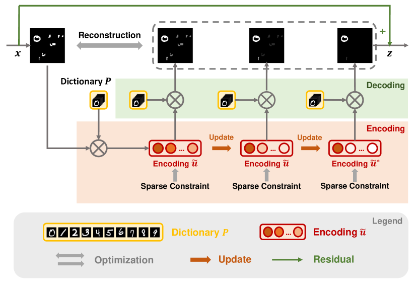
Figure 2: Overview of VARS. First, we initialize $\widetilde{\mathbf{u}}$ as $\mathbf{P}^{T}\mathbf{x}$, the encoding of the input. Then, for each iteration, we update $\widetilde{\mathbf{u}}$ to minimize the reconstruction error between $\mathbf{x}$ and the decoded $\mathbf{P}\widetilde{\mathbf{u}}$, as well as the sparsity constraint. After multiple steps, the converged $\widetilde{\mathbf{u}}^{\ast}$ is decoded and output together with a residual term.

In practice, VARS optimizes the sparse reconstruction (Equation 10) iteratively, as illustrated in Figure 2. First, we initialize $\widetilde{\mathbf{u}}$ as the encoding of input $\mathbf{x}$, i.e., $\widetilde{\mathbf{u}}\leftarrow\mathbf{P}^{T}\mathbf{x}$ (the red block in Figure 2). Then, for each iteration, we decode $\widetilde{\mathbf{u}}$ into $\mathbf{P}\widetilde{\mathbf{u}}$ (the green block in Figure 2) and update $\widetilde{\mathbf{u}}$ by minimizing the reconstruction error $\frac{1}{2}||\mathbf{P}\widetilde{\mathbf{u}}-\mathbf{x}||^{2}_{2}$ and the sparsity constraint $\lambda||\widetilde{\mathbf{u}}||_{1}$. We adopt the update rule in the Iterative Shrinkage Thresholding Algorithm (ISTA) (Beck & Teboulle, 2009), i.e., each update is

$$\small\widetilde{\mathbf{u}}\leftarrow\mathcal{S}_{\frac{\lambda}{L}}\left(\widetilde{\mathbf{u}}-\frac{1}{L}(\mathbf{P}^{T}\mathbf{P}\widetilde{\mathbf{u}}-\mathbf{P}^{T}\mathbf{x})\right),$$ (12)

where $\mathcal{S}_{\lambda}(x)=sgn(x)\cdot(\lvert x\rvert-\lambda)_{+}$ is an element-wise thresholding function, and $L$ is the largest singular value of $\mathbf{P}^{T}\mathbf{P}$. After multiple updates, we decode the converged $\widetilde{\mathbf{u}}^{\ast}$ into $\mathbf{P}\widetilde{\mathbf{u}}^{\ast}$ and output it together with a residual term.

Overall, VARS groups features of different objects in the input into different encoding neurons, and the most salient objects (e.g., “0” in the input in Figure 2) are preserved while other distractors are suppressed by sparse reconstruction. VARS can be easily plugged into any neural network and is computationally efficient thanks to the ISTA algorithm with fast convergence (see Section 4).

3.4 Self-Attention as a Special Case of VARS

Here we show that self-attention can be viewed as a special case of VARS using a dynamic instantiation of the dictionary with single step approximation and no sparsity constraint.

Self-attention formulation. In self-attention, the input $\mathbf{X}\in\mathbb{R}^{N\times C}$ contains $N$ tokens and $C$ channels. We use the superscript $\mu$ for the channel index and the subscript $i$ for the token index, e.g., $\mathbf{X}^{\mu}_{i}$ is the $\mu$-th channel in the $i$-th token. In each head, self-attention gives the output $\mathbf{Z}$ by

$$\small\mathbf{Z}^{\mu}_{i}=\sum_{j}\mathbf{K}(\mathbf{X},\mathbf{X})_{ij}\cdot\mathbf{X}^{\mu}_{j}+\mathbf{X}^{\mu}_{i},$$ (13)

where $\mathbf{K}(\mathbf{X},\mathbf{X})\in\mathbb{R}^{N\times N}$ measures the similarity between tokens in $\mathbf{X}$, i.e., $\mathbf{K}(\mathbf{X},\mathbf{X})_{ij}=e^{(\mathbf{W}\mathbf{X}_{i})^{T}(\mathbf{W}^{\prime}\mathbf{X}_{j})}$, with $\mathbf{W}$ and $\mathbf{W}^{\prime}$ as query and key projections. Self-attention is compute intensive given its quadratic computational complexity. Performer (Choromanski et al., 2020), a recently proposed variant of vision transformers, approximates the similarity kernel with the inner product of the feature maps, i.e., $\mathbf{K}(\mathbf{X},\mathbf{X})\approx\Phi(\mathbf{X})\Phi^{\prime}(\mathbf{X})^{T}$, where $\Phi(\mathbf{X}),\Phi^{\prime}(\mathbf{X})\in\mathbf{R}^{N\times C^{\prime}}$ are specific (random) feature maps of $\mathbf{X}$.

Connection between self-attention and VARS. Following the formulation in Performer, we can rewrite Equation 13 as

$$\small\mathbf{Z}^{\mu}=\Phi(\mathbf{X})\Phi(\mathbf{X})^{T}\mathbf{X}^{\mu}+\mathbf{X}^{\mu}.$$ (14)

Here we use a symmetric similarity kernel by setting $\mathbf{W}=\mathbf{W}^{\prime}$, which means $\Phi=\Phi^{\prime}$. This feed-forward computation is a single-step Euler update of the differential equation

$$\small\derivative{\mathbf{Z}^{\mu}}{t}=-\mathbf{Z}^{\mu}+\Phi(\mathbf{X})\Phi(\mathbf{X})^{T}\mathbf{Z}^{\mu}+\mathbf{X}^{\mu},$$ (15)

which has a similar form with the ODE description of a recurrent layer (Equation 5), except that Equation 15 uses $\Phi(\mathbf{X})$ as the dictionary which is dependent on the specific input $\mathbf{X}$ while Equation 5 uses a static dictionary $\mathbf{P}$ learned from the entire dataset. This shows self-attention is a variant of recurrent networks using a dynamic dictionary. See Appendix A.2 for the visualization of the dynamic dictionary.

However, compared to VARS (Equation 10-11), self-attention (Equation 15) does not have the inhibitive recurrent connections (Equation 9) to turn into sparse reconstruction, and updates the ODE (Equation 15) only via a single step. Therefore, we introduce VARS with a dynamic dictionary:

$$\widetilde{\mathbf{U}}^{\mu^{\ast}} =\operatorname*{arg\,min}_{\widetilde{\mathbf{U}}^{\mu}}\frac{1}{2}||\Phi(\mathbf{X})\widetilde{\mathbf{U}}^{\mu}-\mathbf{X}^{\mu}||^{2}_{2}+2\lambda||\widetilde{\mathbf{U}}^{\mu}||_{1}$$ (16)

$$\mathbf{Z}^{\mu^{\ast}} =\Phi(\mathbf{X})\widetilde{\mathbf{U}}^{\mu^{\ast}}+\mathbf{X}^{\mu},$$ (17)

which optimizes the sparse reconstruction of each channel $\mathbf{X}^{\mu}$ in the input. We refer VARS with a static dictionary to as VARS-S (Equation 10-11) and VARS with an dynamic dictionary as VARS-D (Equation 16-17).

3.5 VARS Instantiations

Dictionary designs. So far, we introduced two instantiations of VARS: VARS with a static dictionary $\mathbf{P}$ (VARS-S) (Equation 10-11) and VARS with a dynamic dictionary $\Phi(\mathbf{X})$ (VARS-D) (Equation 16-17). Both variants have their own merits as $\mathbf{P}$ learns a general pattern of the dataset while $\Phi(\mathbf{X})$ captures the specialized information on a per input basis. Therefore, we consider a third instantiation of VARS, VARS-SD to combine both the static and dynamic dictionaries as $[\mathbf{P};\Phi(\mathbf{X})]$, i.e., using the union of atoms in $\mathbf{P}$ and $\Phi(\mathbf{X})$. We test all three variants in our experiments.

Instantiation of $\mathbf{P}$. In theory, $\mathbf{P}$ can be any real matrix of the specific shape. However, since each column of $\mathbf{P}$ is a template which is a signal in the spatial feature domain, we may impose certain inductive biases such as translational symmetry when instantiating $\mathbf{P}$. To this end, we design $\mathbf{P}$ by making its templates kernels with different translations, which means $\mathbf{P}^{T}$ is a convolution layer, i.e., $(\mathbf{P}^{T}\mathbf{x})_{\uparrow}=\mathit{conv}(\mathbf{x}_{\uparrow})$ where $(\cdot)_{\uparrow}$ unflattens a vector into a 2D signal. Then $\mathbf{P}$ is a deconvolution layer with its kernel shared with the convolution layer, used in both static and static+dynamic dictionaries.

Table 1: Dataset overview. We evaluate VARS on five robustness benchmarks and perform evaluation in three additional settings.

Dataset Name Type Robustness ImageNet-C (IN-C) (Hendrycks & Dietterich, 2019) Natural corruption ImageNet-R (IN-R) (Hendrycks et al., 2021a) Out of distribution ImageNet-SK (IN-SK) (Wang et al., 2019) Out of distribution PGD (Madry et al., 2017) Adversarial attack ImageNet-A (IN-A) (Hendrycks et al., 2021b) Natural adv. example Others PACS (Li et al., 2017) Domain generalization PASCAL VOC (Everingham et al., 2010) Semantic segmentation MIT1003 (Judd et al., 2009) Human eye fixation

4 Experiments

We test VARS on five robustness benchmarks on the ImageNet dataset including naturally corrupted, out of distribution, and adversarial images (Section 4.1). We also evaluate our models on the following settings: domain generalization (Section 4.2), image segmentation, and human eye fixation predictions (Section 4.3). Finally, we analyze and ablate the design choices of VARS in Section 4.4.

Experimental Setup. We evaluate on multiple datasets (Table 1) and the models are pretrained on ImageNet-1K (Deng et al., 2009). For baselines, we consider DeiT (Touvron et al., 2021), a commonly-used vision transformer model, and RVT (Mao et al., 2021), the state-of-the-art vision transformer on various robustness benchmarks. For generality, we also test on GFNet (Rao et al., 2021) using a linear token-mixer instead of self-attention. We apply VARS in the baselines by replacing the global operators (self-attention or token mixer). For all the models, we adopt the convolutional patch-embedding  (Xiao et al., 2021) to facilitate training and also apply Performer approximation which VARS is also built on. We use $\ast$ to denote the modified baselines. Results of both original and modified baselines are reported.

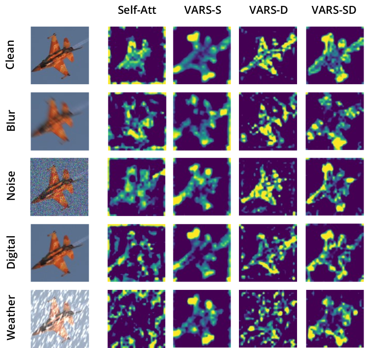
Figure 3: Attention maps under image corruption. We can see VARS consistently highlights the core parts of the object (airplane) while self-attention can miss them (e.g., weather). The attention maps of VARS-SD are most stable and sharp.

Table 2: Evaluation results on robustness benchmarks. We find that VARS consistently improves over the self-attention counterparts (DeiT^∗, GFNet^∗ and RVT^∗). VARS-SD outperforms or is on par with previous methods despite using a weaker initial model. The best performance of each vision transformer architecture is bold and the underlined values are the overall state-of-the-art performance.

Model GFLOPs Params.(M) Clean$\uparrow$ IN-C$\downarrow$ IN-R$\uparrow$ IN-SK$\uparrow$ PGD$\uparrow$ IN-A$\uparrow$ CNNs RegNetY-4GF (Radosavovic et al., 2020) 4.0 20.6 79.2 68.7 38.8 25.9 2.4 8.9 ResNet50 (He et al., 2016) 4.1 25.6 79.0 65.5 42.5 31.5 12.5 5.9 ResNeXt50-32x4d (Xie et al., 2017) 4.3 25.0 79.8 64.7 41.5 29.3 13.5 10.7 InceptionV3 (Szegedy et al., 2016) 5.7 27.2 77.4 80.6 38.9 27.6 3.1 10.0 Transformers PiT-Ti (Heo et al., 2021) 0.7 4.9 72.9 69.1 34.6 21.6 5.1 6.2 ConViT (d’Ascoli et al., 2021) 1.4 5.7 73.3 68.4 35.2 22.4 7.5 8.9 PVT (Wang et al., 2021a) 1.9 13.2 75.0 79.6 33.9 21.5 0.5 7.9 DeiT (Touvron et al., 2021) 1.3 5.7 72.2 71.1 32.6 20.2 6.2 7.3 GFNet (Rao et al., 2021) 1.3 7.5 74.6 65.9 40.4 27.0 7.6 6.3 RVT (Mao et al., 2021) 1.3 8.6 78.4 58.2 43.7 30.0 11.7 13.3 DeiT^∗ 1.3 5.7 74.7 67.0 34.5 21.7 11.9 9.4 w/ VARS-S 1.0 6.8 73.7 69.8 36.8 24.8 10.8 4.9 w/ VARS-D 1.4 5.4 75.6 64.9 39.6 27.5 13.7 10.2 w/ VARS-SD 1.4 5.8 76.5 62.5 40.2 27.5 13.4 11.5 GFNet-Ti^∗ 1.3 7.5 74.6 65.9 40.4 27.0 7.6 6.3 w/ VARS-S 1.3 7.5 74.1 63.5 40.8 28.6 9.5 5.8 w/ VARS-D 1.9 9.8 77.8 58.6 41.2 29.0 15.9 12.6 w/ VARS-SD 1.9 10.4 78.2 57.4 41.0 29.5 16.2 13.0 RVT^∗ 1.3 8.6 77.6 60.4 41.7 28.7 11.1 11.1 w/ VARS-S 1.0 9.2 76.8 61.8 43.2 30.1 7.6 9.1 w/ VARS-D 1.2 8.0 78.2 58.7 42.0 29.8 11.7 12.4 w/ VARS-SD 1.5 9.2 78.4 58.3 42.5 30.5 11.4 13.4

4.1 Evaluation on Robustness Benchmarks

We show the evaluation results on the robustness benchmarks in Table 2. First, we can see vision transformers are generally more robust than the CNN counterparts even with an order of magnitude smaller numbers of parameters and FLOPs. We can also observe that VARS consistently improves the baselines across different benchmarks. For example, compared to DeiT, VARS-SD reduces the error rate from 67% to 62.5% on IN-C and improves the accuracy from 34.5% to 40.2% on IN-R, from 21.7% to 27.5% on IN-SK, which are over 5 absolute points improvements. Similar results are observed with GFNet and RVT.

Moreover, when built on top of the RVT network design, VARS-SD outperforms or is on par with the previous methods across the five benchmarks. Note that VARS is built upon RVT^∗, the modified version of RVT (see Experimental Setup). As shown in Table 2, RVT^∗ has weaker initial performance than the vanilla RVT model, mainly due to the Performer approximation of the self-attention.

In Figure 3, we visualize the attention maps of self-attention and VARS-S,-D,-SD under different image corruption scenarios. We see that for a clean image, all the attention designs can roughly locate salient regions around the main object (airplane). However, self-attention only highlights the center part of the object while VARS-SD and VARS-D capture the contour of the object more clearly. For corrupted images, we observe that attention maps from vanilla self-attention tend to be noisier than VARS. For example, with severe weather corruption (the last row), self-attention misses the main object and rather highlights the snow effect, while VARS-SD still captures the object and suppresses the noise. We also notice that VARS-S tend to produce a blurrier attention map compared to the ones with a dynamic dictionary, which might be due to the weaker expressivity of static dictionary compared to the dynamic dictionary.

Table 3: Evaluation of domain generalization on PACS. Our VARS-SD outperforms the baseline RVT^∗ and other variants.

Target Photo Sketch Cartoon Art RVT^∗ 94.19 81.73 79.78 81.25 VARS-S 93.89 82.62 80.16 81.49 VARS-D 96.29 80.40 80.33 84.77 VARS-SD 96.47 82.78 80.98 86.08

4.2 Evaluation on Domain Generalization

Domain generalization is a related setting, which evaluates the models’ generalization to unseen domains at test time. Here we finetune the ImageNet-pretrained models on three source domains in PACS (Li et al., 2017) and test them on the left-out target domain.

Table 3 shows that VARS-SD outperforms the RVT baseline across all four target domains. Specifically, VARS-SD improves RVT^∗ from 81.25% to 86.08% on the Art domain and from 94.19% to 96.47% on the Photo domain. These results indicate that our attention module is more robust than self-attention when generalizing to unseen domains.

Table 4: Segmentation evaluation on PASCAL VOC using attention maps. Our VARS-SD improves the mean IOU score of the baseline RVT^∗ and is more selective (higher FN scores).

RVT* VARS-S VARS-D VARS-SD mIoU$\uparrow$ 39.92 43.33 42.03 44.15 FP$\downarrow$ 49.41 23.11 25.23 29.28 FN$\downarrow$ 3.95 12.08 11.77 8.76

4.3 Evaluation on Segmentation and Eye Fixation

Attention as coarse image segmentation. Recently, self-supervised vision transformers (Caron et al., 2021) have been shown to produce attention maps that are similar to the semantic segmentation of foreground objects. Following  Caron et al. (2021), we evaluate RVT^∗ with self-attention and VARS on the validation set of PASCAL VOC 2012 using the model trained on ImageNet-1K. To obtain a segmentation map, we normalize an attention map from the global average of tokens to [0, 1] and use a threshold 0.3 to distinguish foreground objects from the background (class agnostic). The main evaluation metric is mean IoU which evaluates the overlapping area between a predicted segmentation map and the ground truth. We also consider false positive (FP) and false negative (FN) rates as metrics.

Table 4 shows that all three variants of VARS achieve higher mean IoU compared to the self-attention counterpart RVT^∗, where VARS-SD improves the score from 39.92% to 44.15%. Also, the FP rate is substantially reduced by our attention framework, indicating that VARS can effectively filter out distracting information and preserve only the relevant information about the foreground objects. Another observation is that VARS has a higher FN rate, suggesting VARS is more selective than self-attention and emphasize more on the core parts of the objects.

Table 5: Evaluation on human eye fixations. Here our VARS-S achieves the highest score while all variants outperforms RVT^∗.

Metric RVT^∗ VARS-S VARS-D VARS-SD NSS 0.502 0.737 0.632 0.678

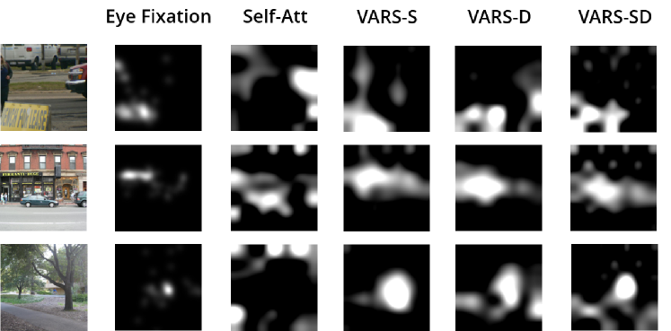
Figure 4: Visualization on eye fixation. VARS’ attention maps are more consistent with human eye fixation than self-attention’s.

Alignment with human eye fixations. Since human eye fixation is under the guidance of bottom-up attention (Li, 2014), here we investigate how close our attention maps are to the human eye fixation maps. Here we evaluate the ImageNet-pretrained RVT with self-attention and VARS on MIT1003 (Judd et al., 2009), containing 1K natural images with eye fixation maps collected from 15 human observers. We adopt the metric of normalized scanpath saliency (NSS) (Peters et al., 2005) that measures an average of normalized attention value at fixated positions.

Table 5 shows that RVT with VARS achieves higher NSS scores than RVT with self-attention (i.e., RVT^∗), aligning better with the human eye fixations data. Figure 4 shows the attention maps captured from humans and generated by the models. We notice that VARS predicts regions that are more closely aligned with human attention, while self-attention tend to highlight irrelevant background regions.

4.4 Analysis and Ablation Study

Recurrent refinement of attention. VARS performs recurrent sparse reconstruction of the inputs in an iterative manner. In Figure 5, we visualize the attention maps VARS-S on ImageNet validation samples at different updating steps. We can see that VARS refines the attention maps through recurrent updates, i.e., the attention maps become more focused on the core parts of the objects while suppressing the background and other distracting objects.

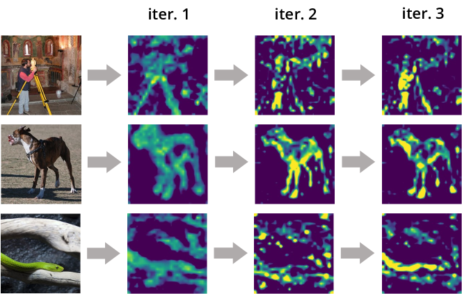
Figure 5: Recurrent refinement of attention maps. VARS refines the attention maps iteratively during the recurrent updates.

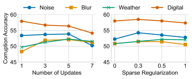
Figure 6: Hyperparameter analysis. We study the number of updates (left) and the level of sparse regularization (right) in sparse reconstruction. VARS performs similarly with 3 to 5 iteration steps and we choose 3 for better efficiency. VARS is not sensitive to the level of sparse regularization and we use 0.3 in the experiments.

Number of recurrent updates. Figure 6 (left) shows the accuracy on ImageNet-C over different number of updates $k$. We find that the model has a similar performance between $k=3$ and $5$ with a drop of performance at $k=1$ and $7$. We choose $k=3$ in our experiments for efficiency.

Strength of sparse constraints. Figure 6 (right) shows the accuracy over different $\lambda$ values that determine the level of sparse regularization during the reconstruction of input. We observe that the curves are relatively flat which indicates VARS is not very sensitive to the strength of the sparse regularization. We adopt $\lambda=0.3$ in our experiments which has a slightly better performance than the other values.

5 Conclusion

We introduced a new attention formulation—Visual Attention from Recurrent Sparse reconstruction (VARS)—which takes inspiration from the robustness characteristics of human vision. We observed a connection among visual attention, recurrency, and sparsity and showed that contemporary attention models can be derived from recurrent sparse reconstruction of input signals. VARS adopts an ODE based formulation to describe neural dynamics; equilibrium states are solved by iteratively optimizing the sparse reconstruction of input. We showed that self-attention is a special case of VARS with approximate neural dynamics and no sparsity constraints. VARS is a general attention module that can be plugged into vision transformers, replacing the self-attention module, offering improved performance. We conducted extensive evaluation on five robustness benchmarks and three additional datasets of related settings to understand the properties of VARS. We found VARS increases model robustness with improved quality of attention maps across various datasets and settings.

Appendix A Additional Qualitative Results

A.1 Evolution of Attention Maps during Recurrent Updates in VARS

In Figure 7 we show more examples of the evolution of attention maps in each step of the recurrent update in VARS. Here we choose VARS-D built upon the RVT baseline and visualize the attention map of the last layer in the first block. We can observe that the attention map is more sharp and concentrated on the salient objects after each iteration.

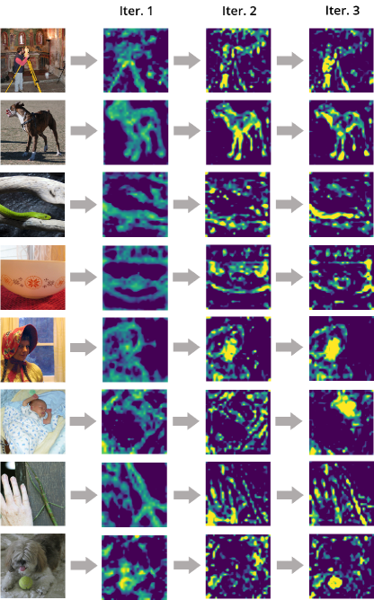
Figure 7: Visualization of the attention maps after each iteration of update in VARS. One can see that the attention will be more concentrated on the salient objects in the image after each update.

A.2 Visualization of Dynamic Dictionaries in VARS-D and VARS-SD

In VARS-D and VARS-SD, we use the input-dependent dictionary $\Phi(\mathbf{X})$ for sparse reconstruction. Here we visualize the dynamic dictionaries for a deeper understanding (Figure 8-10). We can see that most atoms in the dictionary are approximately uniform masks on either foreground or background regions. This is a direct consequence from the design of self-attention and random features (Choromanski et al., 2020).

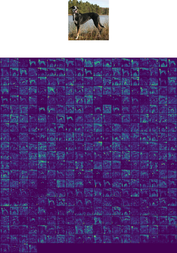
Figure 8: Visualization of the dynamic dictionary. The atoms are mostly masks on either foreground objects or backgrounds.

Figure 9: Visualization of the dynamic dictionary. The atoms are mostly masks on either foreground objects or backgrounds.

Figure 10: Visualization of the dynamic dictionary. The atoms are mostly masks on either foreground objects or backgrounds.

A.3 Visualization of Attention Maps under Different Image Corruptions

We show additional visualization of the attention maps under different image corruptions in Figure 11, where each block contains attention maps of clean images as well as images under noise, blur, digital, and weather corruptions (from top to down). We show the attention maps of RVT^∗, VARS-S, VARS-D, and VARS-SD (from left to right). One can see that the attention maps of self-attention baseline is more sensitive to image corruptions, while variants of VARS tend to output stable attention maps. Meanwhile, the attention maps of VARS-S are steady but not as sharp as VARS-D and VARS-SD.

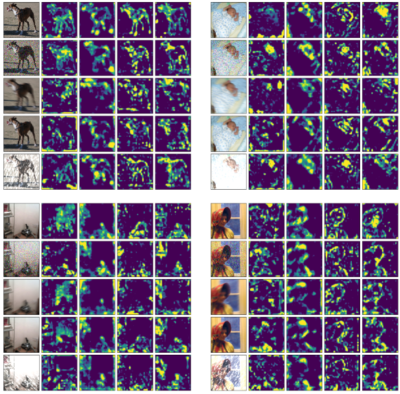
Figure 11: Visualization of the attention maps under image corruptions. Each block contains clean images as well as images under corruption of noise, blur, digital, and weather (from top to down). We visualize the attention map of RVT^∗, VARS-S, VARS-D, and VARS-SD (from left to right in each block). Across different images, self-attention is usually more unstable than the variants of VARS. Meanwhile, VARS-S has attention maps that are consistent under different corruptions but are not as sharp as those of VARS-D and VARS-SD.

A.4 Comparing Attention Maps with Human Eye Fixation

In Figure 12 we show addtional results on comparing the attention maps of different models with the human eye fixation data. We can see that, the attention maps of VARS are more consistent with human eye fixation than self-attention.

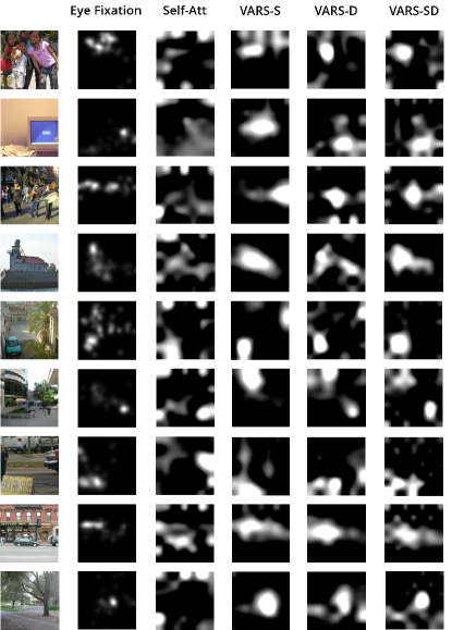
Figure 12: Comparison between attention maps of different models and human eye fixation probabilities. The variants of VARS have attention maps that are more consistent with human eye fixation.

Appendix B Details on Derivation of the Sparse Reconstruction Problem

We follow Rozell et al. (2008) and add recurrent connections between $\mathbf{u}$, modeled by the weight matrix $-\gamma(\mathbf{P}^{T}\mathbf{P}-\mathbf{I})$. We also add hyperparameters $\alpha$ and $\beta$ to control the strength of self-leakage and the element-wise activation functions $\mathit{g}(\cdot)$ to gate the output from the neurons (Dayan & Abbott, 2001). As a result, we fix the dynamics of the recurrent networks as:

$$\derivative{\mathbf{z}}{t}=-\alpha\mathbf{z}+\mathbf{P}\mathit{g}(\mathbf{u})+\mathbf{x},$$ (18)

$$\derivative{\mathbf{u}}{t}=-\beta\mathbf{u}-\gamma(\mathbf{P}^{T}\mathbf{P}-\mathbf{I})\mathit{g}(\mathbf{u})+\mathbf{P}^{T}\mathbf{z}.$$ (19)

By taking $\alpha=1$ and $\beta=\gamma=2$, it has the same steady state solution as

$$\derivative{\mathbf{u}}{t} =-2(\mathbf{u}-\widetilde{\mathbf{u}})-\mathbf{P}^{T}\mathbf{P}\widetilde{\mathbf{u}}+\mathbf{P}^{T}\mathbf{x},$$ (20)

$$\mathbf{z} =\mathbf{P}\widetilde{\mathbf{u}}+\mathbf{x},$$ (21)

where $\widetilde{\mathbf{u}}=\mathit{g}(\mathbf{u})$. Now we choose $\mathit{g}(\cdot)$ as the thresholding function $\mathit{g}(\mathbf{u}_{i})=\mathit{sgn}(\mathbf{u}_{i})\cdot(\lvert\mathbf{u}_{i}\rvert-\lambda)_{+}$, where $\mathit{sgn}(\cdot)$ is the sign function and $(\cdot)_{+}$ is ReLU. Under the assumption that $\mathit{g}(\cdot)$ is monotonically non-decreasing, Eq. 20 is actually minimizing the energy function

$$\small E(\widetilde{\mathbf{u}})=\frac{1}{2}||\mathbf{P}\widetilde{\mathbf{u}}-\mathbf{x}||^{2}+2\lambda||\widetilde{\mathbf{u}}||_{1}.$$ (22)

To see this, one can verify that when $\mathbf{u}$ evolves by Eq. 20, $E(\widetilde{\mathbf{u}})$ is non-increasing, i.e.,,

$$\small\derivative{E}{t}=-(2\lambda\cdot\mathit{sgn}(\mathbf{u})+\mathbf{P}^{T}\mathbf{P}\widetilde{\mathbf{u}}-\mathbf{P}^{T}\mathbf{x})^{T}\cdot\mathbf{K}(\mathbf{u})\cdot(2\lambda\cdot\mathit{sgn}(\mathbf{u})+\mathbf{P}^{T}\mathbf{P}\widetilde{\mathbf{u}}-\mathbf{P}^{T}\mathbf{x})=(\derivative{\mathbf{u}}{t})^{T}\mathbf{K}(\mathbf{u})\derivative{\mathbf{u}}{t},$$ (23)

where $\mathbf{K}(\mathbf{u})$ is a diagonal matrix with $\mathbf{K}(\mathbf{u})_{ii}=1$ when (i) $|\mathbf{u}_{i}|>1$, and (ii) $|\mathbf{u}_{i}|=1$ and $\derivative{\mathbf{u}_{i}}{t}\cdot\mathit{sgn}(\mathbf{u}_{i})>0$, otherwise $\mathbf{K}(\mathbf{u})_{ii}=0$. Since $\mathbf{K}(\mathbf{u})$ is positive semi-definite, Eq. 23 is non-positive, which means the energy is non-increasing. Then Eq. 20 equivalently optimizes the sparse reconstruction:

$$\widetilde{\mathbf{u}}^{\ast} =\operatorname*{arg\,min}_{\widetilde{\mathbf{u}}\in\mathbb{R}^{d^{\prime}}}\frac{1}{2}||\mathbf{P}\widetilde{\mathbf{u}}-\mathbf{x}||^{2}+2\lambda||\widetilde{\mathbf{u}}||_{1}$$ (24)

$$\mathbf{z}^{\ast} =\mathbf{P}\widetilde{\mathbf{u}}^{\ast}+\mathbf{x}.$$ (25)

References

- Bai et al. (2019) Bai, S., Kolter, J. Z., and Koltun, V. Deep equilibrium models. arXiv preprint arXiv:1909.01377, 2019.
- Beck & Teboulle (2009) Beck, A. and Teboulle, M. A fast iterative shrinkage-thresholding algorithm for linear inverse problems. SIAM journal on imaging sciences, 2(1):183–202, 2009.
- Biederman (1987) Biederman, I. Recognition-by-components: a theory of human image understanding. Psychological review, 94(2):115, 1987.
- Bisanz et al. (2012) Bisanz, J., Bisanz, G. L., and Kail, R. Learning in children: Progress in cognitive development research. Springer Science & Business Media, 2012.
- Bosking et al. (1997) Bosking, W. H., Zhang, Y., Schofield, B., and Fitzpatrick, D. Orientation selectivity and the arrangement of horizontal connections in tree shrew striate cortex. Journal of neuroscience, 17(6):2112–2127, 1997.
- Caron et al. (2021) Caron, M., Touvron, H., Misra, I., Jégou, H., Mairal, J., Bojanowski, P., and Joulin, A. Emerging properties in self-supervised vision transformers. arXiv preprint arXiv:2104.14294, 2021.
- Chaney et al. (2014) Chaney, W., Fischer, J., and Whitney, D. The hierarchical sparse selection model of visual crowding. Frontiers in integrative neuroscience, 8:73, 2014.
- Choromanski et al. (2020) Choromanski, K., Likhosherstov, V., Dohan, D., Song, X., Gane, A., Sarlos, T., Hawkins, P., Davis, J., Mohiuddin, A., Kaiser, L., et al. Rethinking attention with performers. arXiv preprint arXiv:2009.14794, 2020.
- Cohen & Grossberg (1983) Cohen, M. A. and Grossberg, S. Absolute stability of global pattern formation and parallel memory storage by competitive neural networks. IEEE transactions on systems, man, and cybernetics, (5):815–826, 1983.
- Darrell et al. (1990) Darrell, T., Sclaroff, S., and Pentland, A. Segmentation by minimal description. In Proceedings Third International Conference on Computer Vision, pp. 112–113. IEEE Computer Society, 1990.
- d’Ascoli et al. (2021) d’Ascoli, S., Touvron, H., Leavitt, M., Morcos, A., Biroli, G., and Sagun, L. Convit: Improving vision transformers with soft convolutional inductive biases. arXiv preprint arXiv:2103.10697, 2021.
- Dayan & Abbott (2001) Dayan, P. and Abbott, L. F. Theoretical neuroscience: computational and mathematical modeling of neural systems. Computational Neuroscience Series, 2001.
- Deng et al. (2009) Deng, J., Dong, W., Socher, R., Li, L.-J., Li, K., and Fei-Fei, L. Imagenet: A large-scale hierarchical image database. In IEEE conference on computer vision and pattern recognition, 2009.
- Desimone & Duncan (1995) Desimone, R. and Duncan, J. Neural mechanisms of selective visual attention. Annual review of neuroscience, 18(1):193–222, 1995.
- Djolonga et al. (2021) Djolonga, J., Yung, J., Tschannen, M., Romijnders, R., Beyer, L., Kolesnikov, A., Puigcerver, J., Minderer, M., D’Amour, A., Moldovan, D., et al. On robustness and transferability of convolutional neural networks. In Proceedings of the IEEE/CVF Conference on Computer Vision and Pattern Recognition, pp. 16458–16468, 2021.
- Dodge & Karam (2017) Dodge, S. and Karam, L. A study and comparison of human and deep learning recognition performance under visual distortions. In 2017 26th international conference on computer communication and networks (ICCCN), pp. 1–7. IEEE, 2017.
- Dong et al. (2020) Dong, M., Li, Y., Wang, Y., and Xu, C. Adversarially robust neural architectures. arXiv preprint arXiv:2009.00902, 2020.
- Dosovitskiy et al. (2020) Dosovitskiy, A., Beyer, L., Kolesnikov, A., Weissenborn, D., Zhai, X., Unterthiner, T., Dehghani, M., Minderer, M., Heigold, G., Gelly, S., et al. An image is worth 16x16 words: Transformers for image recognition at scale. arXiv preprint arXiv:2010.11929, 2020.
- Everingham et al. (2010) Everingham, M., Van Gool, L., Williams, C. K., Winn, J., and Zisserman, A. The pascal visual object classes (voc) challenge. IJCV, 88(2):303–338, 2010.
- Fan et al. (2020) Fan, Y., Yu, J., Mei, Y., Zhang, Y., Fu, Y., Liu, D., and Huang, T. S. Neural sparse representation for image restoration. arXiv preprint arXiv:2006.04357, 2020.
- Felleman & Van Essen (1991) Felleman, D. J. and Van Essen, D. C. Distributed hierarchical processing in the primate cerebral cortex. Cerebral cortex (New York, NY: 1991), 1(1):1–47, 1991.
- Geirhos et al. (2017) Geirhos, R., Janssen, D. H., Schütt, H. H., Rauber, J., Bethge, M., and Wichmann, F. A. Comparing deep neural networks against humans: object recognition when the signal gets weaker. arXiv preprint arXiv:1706.06969, 2017.
- Geirhos et al. (2018) Geirhos, R., Rubisch, P., Michaelis, C., Bethge, M., Wichmann, F. A., and Brendel, W. Imagenet-trained cnns are biased towards texture; increasing shape bias improves accuracy and robustness. arXiv preprint arXiv:1811.12231, 2018.
- Gilbert & Wiesel (1989) Gilbert, C. D. and Wiesel, T. N. Columnar specificity of intrinsic horizontal and corticocortical connections in cat visual cortex. Journal of Neuroscience, 9(7):2432–2442, 1989.
- Grossberg & Mingolla (1987) Grossberg, S. and Mingolla, E. Neural dynamics of perceptual grouping: Textures, boundaries, and emergent segmentations. In The adaptive brain II, pp. 143–210. Elsevier, 1987.
- Guo et al. (2018) Guo, Y., Zhang, C., Zhang, C., and Chen, Y. Sparse dnns with improved adversarial robustness. arXiv preprint arXiv:1810.09619, 2018.
- He et al. (2015) He, K., Zhang, X., Ren, S., and Sun, J. Delving deep into rectifiers: Surpassing human-level performance on imagenet classification. In Proceedings of the IEEE international conference on computer vision, pp. 1026–1034, 2015.
- He et al. (2016) He, K., Zhang, X., Ren, S., and Sun, J. Deep residual learning for image recognition. In Proceedings of the IEEE conference on computer vision and pattern recognition, pp. 770–778, 2016.
- Hendrycks & Dietterich (2019) Hendrycks, D. and Dietterich, T. Benchmarking neural network robustness to common corruptions and perturbations. arXiv preprint arXiv:1903.12261, 2019.
- Hendrycks et al. (2021a) Hendrycks, D., Basart, S., Mu, N., Kadavath, S., Wang, F., Dorundo, E., Desai, R., Zhu, T., Parajuli, S., Guo, M., et al. The many faces of robustness: A critical analysis of out-of-distribution generalization. In Proceedings of the IEEE/CVF International Conference on Computer Vision, pp. 8340–8349, 2021a.
- Hendrycks et al. (2021b) Hendrycks, D., Zhao, K., Basart, S., Steinhardt, J., and Song, D. Natural adversarial examples. In Proceedings of the IEEE/CVF Conference on Computer Vision and Pattern Recognition, pp. 15262–15271, 2021b.
- Heo et al. (2021) Heo, B., Yun, S., Han, D., Chun, S., Choe, J., and Oh, S. J. Rethinking spatial dimensions of vision transformers. arXiv preprint arXiv:2103.16302, 2021.
- Hochreiter & Schmidhuber (1997) Hochreiter, S. and Schmidhuber, J. Long short-term memory. Neural computation, 9(8):1735–1780, 1997.
- Hoefler et al. (2021) Hoefler, T., Alistarh, D., Ben-Nun, T., Dryden, N., and Peste, A. Sparsity in deep learning: Pruning and growth for efficient inference and training in neural networks. arXiv preprint arXiv:2102.00554, 2021.
- Hopfield (1984) Hopfield, J. J. Neurons with graded response have collective computational properties like those of two-state neurons. Proceedings of the national academy of sciences, 81(10):3088–3092, 1984.
- Huang et al. (2020) Huang, Y., Gornet, J., Dai, S., Yu, Z., Nguyen, T., Tsao, D. Y., and Anandkumar, A. Neural networks with recurrent generative feedback. arXiv preprint arXiv:2007.09200, 2020.
- Itti & Koch (2001) Itti, L. and Koch, C. Computational modelling of visual attention. Nature reviews neuroscience, 2(3):194–203, 2001.
- Judd et al. (2009) Judd, T., Ehinger, K., Durand, F., and Torralba, A. Learning to predict where humans look. In 2009 IEEE 12th international conference on computer vision, pp. 2106–2113. IEEE, 2009.
- Kar et al. (2019) Kar, K., Kubilius, J., Schmidt, K., Issa, E. B., and DiCarlo, J. J. Evidence that recurrent circuits are critical to the ventral stream’s execution of core object recognition behavior. Nature neuroscience, 22(6):974–983, 2019.
- Kim et al. (2019) Kim, J., Linsley, D., Thakkar, K., and Serre, T. Disentangling neural mechanisms for perceptual grouping. arXiv preprint arXiv:1906.01558, 2019.
- Koch & Ullman (1987) Koch, C. and Ullman, S. Shifts in selective visual attention: towards the underlying neural circuitry. In Matters of intelligence, pp. 115–141. Springer, 1987.
- Lamme & Roelfsema (2000) Lamme, V. A. and Roelfsema, P. R. The distinct modes of vision offered by feedforward and recurrent processing. Trends in neurosciences, 23(11):571–579, 2000.
- Lee et al. (2007) Lee, H., Ekanadham, C., and Ng, A. Sparse deep belief net model for visual area v2. Advances in neural information processing systems, 20:873–880, 2007.
- Li et al. (2017) Li, D., Yang, Y., Song, Y.-Z., and Hospedales, T. M. Deeper, broader and artier domain generalization. In Proceedings of the IEEE international conference on computer vision, pp. 5542–5550, 2017.
- Li (1998) Li, Z. A neural model of contour integration in the primary visual cortex. Neural computation, 10(4):903–940, 1998.
- Li (2014) Li, Z. Understanding vision: theory, models, and data. Oxford University Press, USA, 2014.
- Linsley et al. (2020) Linsley, D., Kim, J., Ashok, A., and Serre, T. Recurrent neural circuits for contour detection. arXiv preprint arXiv:2010.15314, 2020.
- Liu et al. (2019) Liu, S., Mocanu, D. C., and Pechenizkiy, M. On improving deep learning generalization with adaptive sparse connectivity. arXiv preprint arXiv:1906.11626, 2019.
- Machiraju et al. (2021) Machiraju, H., Choung, O.-H., Frossard, P., Herzog, M., et al. Bio-inspired robustness: A review. arXiv preprint arXiv:2103.09265, 2021.
- Madry et al. (2017) Madry, A., Makelov, A., Schmidt, L., Tsipras, D., and Vladu, A. Towards deep learning models resistant to adversarial attacks. arXiv preprint arXiv:1706.06083, 2017.
- Mao et al. (2021) Mao, X., Qi, G., Chen, Y., Li, X., Duan, R., Ye, S., He, Y., and Xue, H. Towards robust vision transformer. arXiv preprint arXiv:2105.07926, 2021.
- Mély et al. (2018) Mély, D. A., Linsley, D., and Serre, T. Complementary surrounds explain diverse contextual phenomena across visual modalities. Psychological review, 125(5):769, 2018.
- Mnih et al. (2014) Mnih, V., Heess, N., Graves, A., et al. Recurrent models of visual attention. In Advances in neural information processing systems, pp. 2204–2212, 2014.
- Naseer et al. (2021) Naseer, M., Ranasinghe, K., Khan, S., Hayat, M., Khan, F. S., and Yang, M.-H. Intriguing properties of vision transformers. arXiv preprint arXiv:2105.10497, 2021.
- Nayebi et al. (2018) Nayebi, A., Bear, D., Kubilius, J., Kar, K., Ganguli, S., Sussillo, D., DiCarlo, J. J., and Yamins, D. L. Task-driven convolutional recurrent models of the visual system. arXiv preprint arXiv:1807.00053, 2018.
- Olshausen & Field (1996) Olshausen, B. A. and Field, D. J. Emergence of simple-cell receptive field properties by learning a sparse code for natural images. Nature, 381(6583):607–609, 1996.
- Olshausen & Field (1997) Olshausen, B. A. and Field, D. J. Sparse coding with an overcomplete basis set: A strategy employed by v1? Vision research, 37(23):3311–3325, 1997.
- O’Reilly et al. (2013) O’Reilly, R. C., Wyatte, D., Herd, S., Mingus, B., and Jilk, D. J. Recurrent processing during object recognition. Frontiers in psychology, 4:124, 2013.
- Paul & Chen (2021) Paul, S. and Chen, P.-Y. Vision transformers are robust learners. arXiv preprint arXiv:2105.07581, 2021.
- Peters et al. (2005) Peters, R. J., Iyer, A., Itti, L., and Koch, C. Components of bottom-up gaze allocation in natural images. Vision research, 45(18):2397–2416, 2005.
- Radosavovic et al. (2020) Radosavovic, I., Kosaraju, R. P., Girshick, R., He, K., and Dollár, P. Designing network design spaces. In Proceedings of the IEEE/CVF Conference on Computer Vision and Pattern Recognition, pp. 10428–10436, 2020.
- Rao et al. (2021) Rao, Y., Zhao, W., Zhu, Z., Lu, J., and Zhou, J. Global filter networks for image classification. arXiv preprint arXiv:2107.00645, 2021.
- Rebuffi et al. (2021) Rebuffi, S.-A., Gowal, S., Calian, D. A., Stimberg, F., Wiles, O., and Mann, T. A. Data augmentation can improve robustness. Advances in Neural Information Processing Systems, 34, 2021.
- Roelfsema (2006) Roelfsema, P. R. Cortical algorithms for perceptual grouping. Annu. Rev. Neurosci., 29:203–227, 2006.
- Roelfsema et al. (2002) Roelfsema, P. R., Lamme, V. A., Spekreijse, H., and Bosch, H. Figure—ground segregation in a recurrent network architecture. Journal of cognitive neuroscience, 14(4):525–537, 2002.
- Rozell et al. (2008) Rozell, C. J., Johnson, D. H., Baraniuk, R. G., and Olshausen, B. A. Sparse coding via thresholding and local competition in neural circuits. Neural computation, 20(10):2526–2563, 2008.
- Scholl (2001) Scholl, B. J. Objects and attention: The state of the art. Cognition, 80(1-2):1–46, 2001.
- Shi et al. (2020) Shi, B., Zhang, D., Dai, Q., Zhu, Z., Mu, Y., and Wang, J. Informative dropout for robust representation learning: A shape-bias perspective. In International Conference on Machine Learning, pp. 8828–8839. PMLR, 2020.
- Sood et al. (2020) Sood, E., Tannert, S., Frassinelli, D., Bulling, A., and Vu, N. T. Interpreting attention models with human visual attention in machine reading comprehension. arXiv preprint arXiv:2010.06396, 2020.
- Stettler et al. (2002) Stettler, D. D., Das, A., Bennett, J., and Gilbert, C. D. Lateral connectivity and contextual interactions in macaque primary visual cortex. Neuron, 36(4):739–750, 2002.
- Szegedy et al. (2013) Szegedy, C., Zaremba, W., Sutskever, I., Bruna, J., Erhan, D., Goodfellow, I., and Fergus, R. Intriguing properties of neural networks. arXiv preprint arXiv:1312.6199, 2013.
- Szegedy et al. (2016) Szegedy, C., Vanhoucke, V., Ioffe, S., Shlens, J., and Wojna, Z. Rethinking the inception architecture for computer vision. In Proceedings of the IEEE conference on computer vision and pattern recognition, pp. 2818–2826, 2016.
- Tang et al. (2018) Tang, H., Schrimpf, M., Lotter, W., Moerman, C., Paredes, A., Caro, J. O., Hardesty, W., Cox, D., and Kreiman, G. Recurrent computations for visual pattern completion. Proceedings of the National Academy of Sciences, 115(35):8835–8840, 2018.
- Touvron et al. (2021) Touvron, H., Cord, M., Douze, M., Massa, F., Sablayrolles, A., and Jégou, H. Training data-efficient image transformers & distillation through attention. In International Conference on Machine Learning, pp. 10347–10357. PMLR, 2021.
- Vaswani et al. (2017) Vaswani, A., Shazeer, N., Parmar, N., Uszkoreit, J., Jones, L., Gomez, A. N., Kaiser, Ł., and Polosukhin, I. Attention is all you need. In Advances in neural information processing systems, pp. 5998–6008, 2017.
- Vecera & Farah (1997) Vecera, S. P. and Farah, M. J. Is visual image segmentation a bottom-up or an interactive process? Perception & Psychophysics, 59(8):1280–1296, 1997.
- Walther et al. (2005) Walther, D., Rutishauser, U., Koch, C., and Perona, P. Selective visual attention enables learning and recognition of multiple objects in cluttered scenes. Computer Vision and Image Understanding, 100(1-2):41–63, 2005.
- Wang et al. (2019) Wang, H., Ge, S., Xing, E. P., and Lipton, Z. C. Learning robust global representations by penalizing local predictive power. arXiv preprint arXiv:1905.13549, 2019.
- Wang et al. (2021a) Wang, W., Xie, E., Li, X., Fan, D.-P., Song, K., Liang, D., Lu, T., Luo, P., and Shao, L. Pyramid vision transformer: A versatile backbone for dense prediction without convolutions. arXiv preprint arXiv:2102.12122, 2021a.
- Wang et al. (2018) Wang, X., Girshick, R., Gupta, A., and He, K. Non-local neural networks. In Proceedings of the IEEE conference on computer vision and pattern recognition, pp. 7794–7803, 2018.
- Wang et al. (2021b) Wang, X., Huang, T. E., Liu, B., Yu, F., Wang, X., Gonzalez, J. E., and Darrell, T. Robust object detection via instance-level temporal cycle confusion. arXiv preprint arXiv:2104.08381, 2021b.
- Wright et al. (2008) Wright, J., Yang, A. Y., Ganesh, A., Sastry, S. S., and Ma, Y. Robust face recognition via sparse representation. IEEE transactions on pattern analysis and machine intelligence, 31(2):210–227, 2008.
- Wu et al. (2016) Wu, S., Wong, K. M., Fung, C. A., Mi, Y., and Zhang, W. Continuous attractor neural networks: candidate of a canonical model for neural information representation. F1000Research, 5, 2016.
- Wu et al. (2019) Wu, Y., Rosca, M., and Lillicrap, T. Deep compressed sensing. In International Conference on Machine Learning, pp. 6850–6860. PMLR, 2019.
- Wyatte et al. (2012) Wyatte, D., Curran, T., and O’Reilly, R. The limits of feedforward vision: Recurrent processing promotes robust object recognition when objects are degraded. Journal of Cognitive Neuroscience, 24(11):2248–2261, 2012.
- Wyatte et al. (2014) Wyatte, D., Jilk, D. J., and O’Reilly, R. C. Early recurrent feedback facilitates visual object recognition under challenging conditions. Frontiers in psychology, 5:674, 2014.
- Xiao et al. (2021) Xiao, T., Dollar, P., Singh, M., Mintun, E., Darrell, T., and Girshick, R. Early convolutions help transformers see better. Advances in Neural Information Processing Systems, 34, 2021.
- Xie et al. (2017) Xie, S., Girshick, R., Dollár, P., Tu, Z., and He, K. Aggregated residual transformations for deep neural networks. In Proceedings of the IEEE conference on computer vision and pattern recognition, pp. 1492–1500, 2017.
- Yen & Finkel (1998) Yen, S.-C. and Finkel, L. H. Extraction of perceptually salient contours by striate cortical networks. Vision research, 38(5):719–741, 1998.
- Zoran et al. (2020) Zoran, D., Chrzanowski, M., Huang, P.-S., Gowal, S., Mott, A., and Kohli, P. Towards robust image classification using sequential attention models. In Proceedings of the IEEE/CVF conference on computer vision and pattern recognition, pp. 9483–9492, 2020.
- Zucker et al. (1989) Zucker, S. W., Dobbins, A., and Iverson, L. Two stages of curve detection suggest two styles of visual computation. Neural computation, 1(1):68–81, 1989.