The Lack of Convexity of the Relevance-Compression Function

Abstract

In this paper we investigate the convexity of the relevance-compression function for the Information Bottleneck and the Information Distortion problems. This curve is an analog of the rate-distortion curve, which is convex. In the problems we discuss in this paper, the distortion function is not a linear function of the quantizer, and the relevance-compression function is not necessarily convex (concave), but can change its convexity. We relate this phenomena with existence of first order phase transitions in the corresponding Lagrangian as a function of the annealing parameter.

1 Introduction

In previous work [1, 2, 3] we have described the bifurcation structure for solutions to problems of the form

$$\begin{array}[]{c}\max_{q\in\Delta}G(q)\\ D(q)\geq D_{0}\end{array}$$ (3)

where $\Delta$ is a constraint space of valid conditional probabilities, $G$ and $D$ are continuous, real valued functions of $q$, smooth in the interior of $\Delta$, and the functions $G(q)$ and $D(q)$ are invariant under the group of symmetries $S_{N}$. This type of problem, which arises in Rate Distortion Theory [4, 5] and Deterministic Annealing [6], is $NP$ complete [7] when $D(q)$ is the mutual information $I(X;Y_{N})$ as in the Information Bottleneck [8, 9, 10] and the Information Distortion [11, 12, 13] methods. In this paper, we address the relationship between the bifurcation structure of solutions to (3) and the relevance compression function [10].

2 Preliminaries

2.1 Rate Distortion Theory

We assume that the random variable $X\in\{x_{1},x_{2},...,x_{K}\}$ is an input source, and that $Y\in\{y_{1},y_{2},...,y_{K}\}$ is an output source. In rate distortion theory [4], the random variable $Y$ is represented by using $N$ symbols or classes, which we call $Y_{N}$, where we assume without loss of generality that $Y_{N}\in\{1,2,...,N\}$. We denote a stochastic clustering or quantization, of the realizations of $Y$ to the classes of $Y_{N}$, by $q(Y_{N}|Y)$. To find the quantization that yields the minimum information rate $I(Y;Y_{N})$ at a given distortion, one can find points on the rate distortion curve for each value of $D_{0}\in[0,D_{\max}]$. The rate distortion curve is defined as [4, 5]

$$R(D_{0}):=\begin{array}[]{c}\min_{q\in\Delta}I(Y;Y_{N})\\ D(Y,Y_{N})\leq D_{0}\end{array},$$ (6)

where $D(q)$ is a distortion function. A quantization $q(Y_{N}|Y)$ that satisfies (6) yields an approximation of the probabilistic relationship, $p(X,Y)$, between $X$ and $Y$ [11, 8, 9]. The constraint space $\Delta$ is the space of valid finite conditional probabilities $q(Y_{N}|Y)$, where we will write $q(Y_{N}=\nu|Y=y_{k})=q_{\nu k}$.

The Information Bottleneck method [8, 9, 10] uses the information distortion function $D(q):=I(X;Y)-I(X;Y_{N})$. Since the spaces $X$ and $Y$ are fixed, then $I(X;Y)$ is fixed, and so the rate distortion problem (6) in the case of the Information Bottleneck problem can rewritten as

$$R_{I}(I_{0}):=\begin{array}[]{c}\max_{q\in\Delta}-I(Y;Y_{N})\\ I(X;Y_{N})\geq I_{0}\end{array}$$ (9)

where $I_{0}>0$ is some information rate. The function $R_{I}(I_{0})$ is referred to as the relevance-compression function in [10]. Observe that there is a one to one correspondence between $I_{0}$ and $D_{0}$ via $I_{0}=I(X;Y)-D_{0}$. To solve the neural coding problem, the Information Distortion method [11, 12, 13] considers a problem of the form

$$R_{H}(I_{0}):=\begin{array}[]{c}\max_{q\in\Delta}H(Y_{N}|Y)\\ I(X;Y_{N})\geq I_{0}\end{array}$$ (12)

where $H(Y_{N}|Y)$ is the conditional entropy.

2.2 Annealing

Using the method of Lagrange multipliers, an arbitrary problem of the form (3) is rewritten as

$$\max_{q\in\Delta}\left(G(q))+\beta(D(q)-D_{0})\right).$$ (13)

As we will see, solutions of (3) are not always solutions of (13). Similarly, the problem (9) can be rewritten [8, 9, 10] as

$$\max_{q\in\Delta}\left(-I(Y_{N},Y)+\beta I(X;Y_{N})\right),$$ (14)

and problem (12) can be rewritten [11, 12, 13], in analogy with Deterministic Annealing [6], as

$$\max_{q\in\Delta}\left(H(Y_{N}|Y)+\beta I(X;Y_{N})\right).$$ (15)

In (13), (14) and (15), the Lagrange multiplier $\beta$ can be viewed as an annealing parameter.

2.3 Bifurcation Structure of solutions

In [14], we presented an algorithm which can be used to determine the bifurcation structure of stationary points of (13) for each value of $\beta\in[0,\beta_{\max})$ for some $\beta_{\max}>0$. These stationary points are quantizers $q^{*}(\beta)\in\Re^{NK}$ where there exists a vector of Lagrange multipliers $\lambda^{*}\in\Re^{K}$ such that the gradient of the Lagrangian of (3) is a vector of 0’s,

$$\nabla_{q,\lambda}(G(q^{*})+\beta D(q^{*})+\sum_{k=1}^{K}\lambda^{*}_{k}(\sum_{\nu}q^{*}(\nu|y_{k})-1)=\boldsymbol{0}.$$

This condition is also known as the Karush-Kuhn-Tucker necessary condition for constrained optimality [15]. It is well known in optimization theory that a stationary point, i.e. the point satisfying (2.3), is a solution of (3) if the matrix of second derivatives, the Hessian $\Delta_{q}(G(q)+\beta D(q))$, is negative definite on the kernel of the Jacobian of the constraints [15]. We have the following results.

Theorem 1

[1] A stationary point $q^{*}$, is a solution of (13) if $\Delta_{q}(G(q^{*})+\beta D(q^{*}))$ is negative definite on $\ker\left(\begin{array}[]{c}I_{K}~{}~{}I_{K}~{}~{}...~{}~{}I_{K}\end{array}\right)$. A stationary point $q^{*}$ is a solution of (3) if $\Delta_{q}(G(q^{*})+\beta D(q^{*}))$ is negative definite on $\ker\left(\begin{array}[]{c}\nabla_{q}D(q^{*})^{T}\\ I_{K}~{}~{}I_{K}~{}~{}...~{}~{}I_{K}\end{array}\right)$.

From Theorem 1 we see that there may be solutions of (3) which are not solutions of (13). We illustrate this fact numerically. For the Information Distortion problem (12) [11, 12, 13], and the synthetic data set composed of a mixture of four Gaussians which the authors used in [11], we determined the bifurcation structure of solutions to (12) by annealing in $\beta$ and finding the corresponding stationary points to (15) (see Figure 1).

A	B

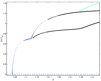
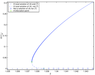
Figure 1: (A) The bifurcation structure of stationary points of the Information Distortion problem (12), a problem of the form (3). We found these points by annealing in $\beta$ and finding stationary points for the problem (15) using the algorithm which we presented in [14]. A square indicates where a bifurcation occurs. (B) A close up of the subcritical bifurcation at $\beta\approx 1.038706$, indicated by an square. Observe the subcritical bifurcating branch, and the subsequent saddle-node bifurcation at $\beta\approx 1.037479$, indicated by another square. We applied Theorem 1 to show that the subcritical bifurcating branch is composed of quantizers which are solutions of (12) but not of (15).

Similar to the results which we presented in [14], the close up of the bifurcation at $\beta\approx 1.038706$ in Figure 1(B) shows a subcritical bifurcating branch (a first order phase transition) which consists of stationary points of the problem (15). By projecting the Hessian $\Delta_{q}(G(q^{*})+\beta D(q^{*}))$ onto each of the kernels referenced in Theorem 1, we determined that the points on this subcritical branch are not solutions of (15), and yet they are solutions of (3).

Furthermore, observe that Figure 1(B) indicates that a saddle-node bifurcation occurs at $\beta\approx 1.037479$. That this is indeed the case was proved in [1]. In fact, for any problem of the form (13), there are only two types of bifurcations to be expected.

A	B

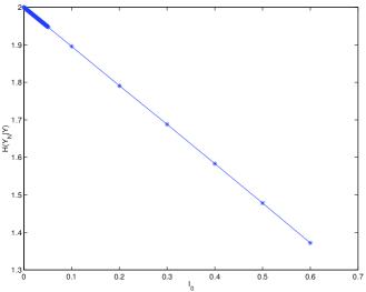
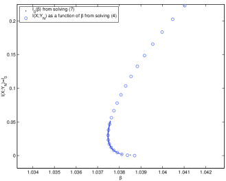
Figure 2: (A) The distortion curve $R_{H}(I_{0})$ defined in (17). For each value of $I_{0}$, we solved the problem (12) to ascertain $H(Y_{N}|Y)$. Observe that the quantizers which yield $I(X;Y_{N})\geq I_{0}$ for the values $I_{0}\in[0,.03]$ correspond to solutions on the subcritical bifurcating branch shown in Figure fig:bifstructure(B). (B) For each value of $I_{0}$, we solved (12), and found the corresponding Lagrange multiplier. This plot shows $I_{0}$ as function of this Lagrange multiplier. This plot is identical to the subcritical bifurcation shown in Figure 1(B), which shows $I(X;Y_{N})$ as a function of the annealing parameter $\beta$.

Theorem 2

[1] Generically, for problems of the form (3), only symmetry breaking pitchfork-like and saddle-node bifurcations occur.

Clearly, the existence of saddle-node bifurcation at $\beta\approx 1.037479$ is tied to the existence of subcritical bifurcation (first order phase transition) at $\beta\approx 1.038706$. We now investigate the connection between existence of subcritical bifurcations and the convexity of the relevance-compression function.

3 The Relevance-Compression Function

Given the generic existence of subcritical pitchfork-like and saddle-node bifurcations of solutions to problems of the form (3), a natural question arises: What are the implications for the rate distortion curve (6)? We examine this question for the information distortion $D(q)=I(X;Y)-I(X;Y_{N})$, used by the Information Bottleneck and the Information Distortion methods. Recall that the relevance-distortion function is

$$R_{I}(I_{0}):=\max_{\Delta\cap{\cal Q}_{I_{0}}}-I(Y_{N},Y).$$ (16)

where

$${\cal Q}_{I_{0}}:=\{q\in\Delta\>|\>I(X,Y_{N})\geq I_{0}\}.$$

For the Information Distortion problem the relevance-distortion function is

$$R_{H}(I_{0}):=\max_{\Delta\cap{\cal Q}_{I_{0}}}H(Y_{N}|Y).$$ (17)

In Figure 2(A), we present a plot of $R_{H}(I_{0})$, which was computed using the same data set of a mixture of four Gaussians which we used in Figures 1(A) and (B). The plot was obtained by solving the problem (12) for each value of $I_{0}$.

To make explicit the relationship between the bifurcation structure shown in Figure 1, which was obtained by annealing in $\beta$, and the distortion curve shown in Figure 2(A), which was obtained by annealing in $I_{0}$, we present Figure 2(B). When solving (12) for each $I_{0}$, we computed the corresponding Lagrange multiplier $\beta$. Thus, $\beta=\beta(I_{0})$, which is the curve we show in Figure 2(B). This plot is matches precisely the subcritical bifurcating branch from Figure 1(B), which we obtained by annealing in $\beta$.

Lemma 3

For a fixed value of $I_{0}>0$ the solution $q^{*}$ of (9) and (12) satisfies the equality constraint $I=I_{0}$.

Proof.      Assume $q^{*}$ is a maximizer of (12) and $I(q^{*})>I_{0}$. Then the constraint is not active and we must have $\nabla H(q^{*})=0$. Since $\nabla H(q^{*})=0$ implies $q^{*}=1/N$, we get $I(q^{*})=0$. This is a contradiction and thus $I(q^{*})=I_{0}$.

Now assume $q^{*}$ is a maximizer of (9) and $I(q^{*})>I_{0}$. Then again the constraint is not active and we must have $\nabla I(Y,Y_{N})=0$. Short computation shows that the condition $\nabla I(Y,Y_{N})=0$ implies $q^{*}=(q_{\nu k})$ is of the form $q_{\nu k}=a_{\nu}$, i.e. $q_{\nu k}$ does not depend on $k$. However, at such value of $q^{*}$ we get $I(q^{*})=0$. This is again a contradiction and thus $I(q^{*})=I_{0}$. $\Box$

As a consequence of the Lemma, for each $I_{0}>0$ there exists a Lagrange multiplier $\beta(I_{0})$. The existence of subcritical bifurcation branch implies that along this branch $\beta(I_{0})$ is not a one-to-one function of $I_{0}$, and therefore not invertible.

3.1 Properties of relevance-compression function

It is well known that if the distortion function $D(q)$ is linear in $q$, that $R(D_{0})$ is a non-increasing and convex [4, 5]. The proof of this result first establishes that the rate-distortion curve is monotone and that it is convex. These two properties together imply continuity and strict monotonicity of the rate distortion curve. Since the information distortion $D=I(X;Y)-I(X;Y_{N})$ is not a linear function of $q$, the convexity proof given in [4, 5] does not generalize to prove that either (16) or (17) is convex. Therefore we need to prove continuity of the relevance-compression function using other means.

Lemma 4

The curves $R_{H}$ and $R_{I}$ are non-increasing curves on $I_{0}\in[0,I_{\max}]$ and are continuous for $I_{0}\in(0,I_{\max})$.

Proof.      Observe that since $I(X,Y_{N})$ is convex [11] in quantizer $q$, we have that

$${\cal Q}_{I_{1}}\subset{\cal Q}_{I_{2}}\mbox{ whenever }I_{1}\geq I_{2}.$$

Therefore, if $I_{1}\geq I_{2}$, then the maximization at $I_{1}$ happens over a smaller set than in $\cal Q_{I_{2}}$, and so $R(I_{1})\leq R(I_{2})$.

Now we prove continuity. Take an arbitrary $I_{0}\in(0,I_{\max})$. Let

$$M_{I_{0}}:=\{y\>|\>y=H(q)\mbox{ where }q\in\Delta\cap{\cal Q}_{D_{0}}\}$$

be the range (in ${\rm I\kern-1.6pt{\rm R}}$) of the function $H(q)$ with the domain $\Delta\cap{\cal Q}_{I_{0}}$. Given an arbitrary $\epsilon>0$, let $M^{\epsilon}_{I_{0}}$ be an $\epsilon$ neighborhood of $M_{I_{0}}$ in ${\rm I\kern-1.6pt{\rm R}}$. A direct computation shows that $\nabla_{q}H(q)=\boldsymbol{0}$ if and only if $q$ is homogeneous, i.e. $qnuk=1/N$, where $N$ is the number of classes of $Y_{N}$. Since $H(q)$ is continuous on $\Delta$, then the set $H^{-1}(M^{\epsilon}_{I_{0}})$ is a relatively open set in $\Delta$. Because by definition $H(\Delta\cap{\cal Q}_{I_{0}})=M_{I_{0}}$, we see that

$${\cal Q}_{I_{0}}\cap\Delta\subset H^{-1}(M^{\epsilon}_{I_{0}}).$$ (18)

Furthermore, since $\nabla H(q)\neq 0$ for $q\in{\cal Q}_{I_{0}}$, then, by the Inverse Mapping Theorem, $H^{-1}(M^{\epsilon}_{I_{0}})$ is an open neighborhood of ${\cal Q}_{I_{0}}$.

The function $I(X;Y_{N})$ is also continuous in the interior of $\Delta$. Observe that

$${\cal Q}_{I_{0}}=I^{-1}([I_{0},I_{\max}])$$

is closed, and thus ${\cal Q}_{I_{0}}\cap\Delta$ is closed and hence compact. Thus, by (18) $H^{-1}(M^{\epsilon}_{I_{0}})$ is an relatively open neighborhood of a compact set ${\cal Q}_{I_{0}}\cap\Delta$. Therefore, since $I(X;Y_{N})$ is continuous, there exists a $\delta>0$ such that the set

$${\rm Int}{\cal Q}_{I_{0}+\delta}\cap\Delta=I^{-1}((I_{0}+\delta,D_{\max}])\cap\Delta$$

is a relatively open set in $\Delta$ such that

$${\cal Q}_{I_{0}}\cap\Delta\subset{\rm Int}{\cal Q}_{I_{0}+\delta}\subset H^{-1}(M^{\epsilon}_{I_{0}}).$$

It then follows that

$$|\max_{\Delta\cap{\cal Q}_{I_{0}+\delta}}H-\max_{\Delta\cap{\cal Q}_{I_{0}}}H|<\epsilon.$$

By definition of the rate distortion function, this means that

$$|R(I)-R(I_{0})|<\epsilon\mbox{ whenever }I-I_{0}<\delta.$$

Since $\epsilon$ was arbitrary, this implies continuity of $R(I)$ at $I=I_{0}$. $\Box$

3.2 The Derivative $\frac{\partial R}{\partial I_{0}}$

In [8, 10], using variational notation, it is shown that

$$\frac{\delta R_{I}}{\delta D}=-\beta.$$

For the sake of completeness, we will reprove this, acknowledging explicitly the fact that the problems (9) and (12) are constrained problems.

Theorem 5

If relevance-compression functions $R_{I}(I_{0})$ and $R_{H}(I_{0})$ are differentiable, then

$$\frac{dR}{dI_{0}}=-\beta(I_{0})\mbox{ and }\frac{d^{2}R}{dI_{0}^{2}}=-\frac{d\beta(I_{0})}{dI_{0}}$$ (19)

Corollary 6

Since $\frac{d\beta(I_{0})}{dI_{0}}$ changes sign at saddle-node bifurcation, then the relevance-compression functions $R_{I}(I_{0})$ and $R_{H}(I_{0})$ are neither concave, nor convex.

Proof of Theorem 5: We start with

$$\max_{q\in\Delta}R(q)+\beta D(q)+\sum_{k}\lambda_{k}(\sum_{\nu}q_{\nu k}-1),$$ (20)

where $R(q)$ is one of $R_{I}(q):=H(Y_{N}|Y),R_{H}(q):=-I(Y_{N},Y)$. We parameterize the solution $q^{*}$ locally by $\beta$. This can be done everywhere except if $q^{*}$ is at a saddle-node bifurcation. At $q^{*}(\beta)$,

$$\nabla_{q}R+\beta\nabla_{q}D+\vec{\lambda}=0.$$ (21)

Lemma 7

For $q\in\Delta$,

$$q\cdot\nabla_{q}R_{H}=R_{H}+1,~{}~{}q\cdot\nabla_{q}R_{I}=R_{I},\mbox{ and }q\cdot\nabla_{q}I=I.$$ (22)

Proof.      Direct calculation. $\Box$

Hence (21) implies

$$R(q^{*}(\beta))+c+\beta I(q^{*}(\beta))+q\cdot\vec{\lambda}=0$$ (23)

Here $c=1$ for $R_{H}$ and $c=0$ for $R_{I}$ is a constant. For $q\in\Delta$, we set

$$\Lambda(\beta):=q\cdot\vec{\lambda}=\sum_{k}\lambda_{k}.$$

The equation (23) defines a relation between $R$ and $I$. Recall, that we can always express $\beta=\beta(I_{0})$. Then the term $I(q^{*}(\beta(I_{0})))=I_{0}$ and we have a relationship

$$R(I_{0})+c+\beta(I_{0})I_{0}+\Lambda(I_{0})=0.$$ (24)

We differentiate (24):

$$\frac{dR}{dI_{0}}+\frac{d\beta}{dI_{0}}I_{0}+\beta(I_{0})+\frac{d\Lambda}{dI_{0}} = 0\Rightarrow$$ (25)

which shows that $\frac{dR}{dI_{0}}=-\frac{d\beta}{dI_{0}}(I_{0}+\frac{d\Lambda}{d\beta})-\beta(I_{0})$ since $\frac{d\Lambda}{dI_{0}}=\frac{d\Lambda}{d\beta}\frac{d\beta}{dI_{0}}$.

In [11](equation (10)) we have an explicit expression for $\lambda_{k}$ as a function of $\beta$:

$$\lambda_{k}=p_{k}(1-{\rm ln}\sum_{\nu}e^{\beta(\nabla I)_{\nu k}/p_{k}}).$$ (26)

Differentiating this with respect to $\beta$ yields

$$\frac{d\lambda_{k}}{d\beta}=-p_{k}\frac{\sum_{\nu}e^{\beta(\nabla I)_{\nu k}/p_{k}}(\nabla I)_{\nu k}/p_{k}}{\sum_{\nu}e^{\beta(\nabla I)_{\nu k}/p_{k}}}.$$

Since $\Lambda=\sum_{k}\lambda_{k}$, this implies that

$$\frac{d\Lambda}{d\beta} = \sum_{k}\frac{d\lambda_{k}}{d\beta}=-\sum_{\nu k}\frac{e^{\beta(\nabla I)_{\nu k}/p_{k}}}{\sum_{\mu}e^{\beta(\nabla I)_{\mu k}/p_{k}}}(\nabla I)_{\nu k}$$

For a solution $q^{*}$, $\frac{e^{\beta(\nabla I)_{\nu k}/p_{k}}}{\sum_{\mu}e^{\beta(\nabla I)_{\mu k}/p_{k}}}=q^{*}_{\nu k}$ ([11], (12)), hence

$$\frac{d\Lambda}{d\beta}|_{q^{*}}=-\sum_{\nu k}q^{*}_{\nu k}(\nabla I)_{\nu k}=-q^{*}\cdot\nabla I=-I$$

This shows that the term $I_{0}+\frac{d\Lambda}{d\beta}=0$ at $q^{*}$, hence from (25) we get the first part of (19). The second part follows immediately. $\Box$

Acknowledgments

This research is partially supported by NSF grants DGE 9972824, MRI 9871191, and EIA-0129895; and NIH Grant R01 MH57179.

References

- [1] Albert E. Parker and Tomas Gedeon. Bifurcations of a class of Sn-invariant constrained optimization problems. Journal of Dynamics and Differential Equations, 16(3):629–678, July 2004. Second special issue dedicated to Shui-Nee Chow.
- [2] A Parker, A Dimitrov, and T Gedeon. Symmetry breaking clusters in soft clustering decoding of neural codes. IEEE Trans. Inform. Theor., 56:901–927, 2010.
- [3] T. Gedeon, A. Parker, and A. Dimitrov. The mathematical structure of information bottleneck methods. Entropy: Special issue for the Information Bottleneck Method, 14:456–479, 2012.
- [4] Thomas Cover and Jay Thomas. Elements of Information Theory. Wiley Series in Communication, New York, 1991.
- [5] Robert M. Gray. Entropy and Information Theory. Springer-Verlag, 1990.
- [6] Kenneth Rose. Deteministic annealing for clustering, compression, classification, regression, and related optimization problems. Proc. IEEE, 86(11):2210–2239, 1998.
- [7] Brendan Mumey and Tomas Gedeon. Optimal mutual information quantization is np-complete. Neural Information Coding (NIC) workshop, Snowbird UT, 2003.
- [8] Noam Slonim and Naftali Tishby. Agglomerative information bottleneck. In S. A. Solla, T. K. Leen, and K.-R. Muller, editors, Advances in Neural Information Processing Systems, volume 12, pages 617–623. MIT Press, 2000.
- [9] Naftali Tishby, Fernando C. Pereira, and William Bialek. The information bottleneck method. The 37th annual Allerton Conference on Communication, Control, and Computing, 1999.
- [10] Noam Slonim. The information bottleneck: Theory and applications. Doctoral Thesis, Hebrew University, 2002.
- [11] Alexander G. Dimitrov and John P. Miller. Neural coding and decoding: communication channels and quantization. Network: Computation in Neural Systems, 12(4):441–472, 2001.
- [12] Alexander G. Dimitrov and John P. Miller. Analyzing sensory systems with the information distortion function. In Russ B Altman, editor, Pacific Symposium on Biocomputing 2001. World Scientific Publishing Co., 2000.
- [13] Tomas Gedeon, Albert E. Parker, and Alexander G. Dimitrov. Information distortion and neural coding. Canadian Applied Mathematics Quarterly, 10(1):33–70, 2003.
- [14] Albert Parker, Tomas Gedeon, and Alexander Dimitrov. Annealing and the rate distortion problem. In S. Thrun S. Becker and K. Obermayer, editors, Advances in Neural Information Processing Systems 15, volume 15, pages 969–976. MIT Press, Cambridge, MA, 2003.
- [15] J. Nocedal and S. J. Wright. Numerical Optimization. Springer, New York, 2000.