On the $f$-divergences between densities of a multivariate location or scale family

Abstract

We first extend the result of Ali and Silvey [Journal of the Royal Statistical Society: Series B, 28.1 (1966), 131-142] who first reported that any $f$-divergence between two isotropic multivariate Gaussian distributions amounts to a corresponding strictly increasing scalar function of their corresponding Mahalanobis distance. We report sufficient conditions on the standard probability density function generating a multivariate location family and the function generator $f$ in order to generalize this result. This property is useful in practice as it allows to compare exactly $f$-divergences between densities of these location families via their corresponding Mahalanobis distances, even when the $f$-divergences are not available in closed-form as it is the case, for example, for the Jensen-Shannon divergence or the total variation distance between densities of a normal location family. Second, we consider $f$-divergences between densities of multivariate scale families: We recall Ali and Silvey ’s result that for normal scale families we get matrix spectral divergences, and we extend this result to densities of a scale family.

Keywords: $f$-divergence; Jensen-Shannon divergence; multivariate location-scale family; spherical distribution; affine group; multivariate normal distributions; multivariate Cauchy distributions; matrix spectral divergence.

1 Introduction

Let $\mathbb{R}$ denote the real field and $\mathbb{R}_{++}$ the set of positive reals. The $f$-divergence [6, 1] induced by a convex generator $f:\mathbb{R}_{++}\rightarrow\mathbb{R}$ between two probability density functions (PDFs) $p(x)$ and $q(x)$ defined on the full support $\mathbb{R}^{d}$ is defined by

$$I_{f}(p:q):=\int p(x)\,f\left(\frac{q(x)}{p(x)}\right)\,\mathrm{d}x.$$

It follows from Jensen’s inequality that we have

$$I_{f}(p:q)\geq f\left(\int p(x)\frac{q(x)}{p(x)}\mathrm{d}x\right)=f(1).$$

Thus we shall consider convex generators $f(u)$ such that $f(1)=0$. Moreover, in order to ensure that $I_{f}(p:q)=0$ if and only if ${p(x)=q(x)}$ except at countably many points $x$, we need $f(u)$ to be strictly convex at $u=1$. The class of $f$-divergences include the total variation distance (the only $f$-divergence up to scaling which is a metric distance [11]), the Kullback-Leibler divergence (and its two common symmetrizations, namely, the Jeffreys divergence and the Jensen-Shannon divergence), the squared Hellinger divergence, the Pearson and Neyman $\chi^{2}$-divergences, etc. The formula for those statistical divergences with their corresponding generators are listed in Table 1.

$$\begin{array}[]{lll}\text{$f$-divergence }&\text{Formula $I_{f}(p:q)$}&\text{Generator $f(u)$ with $f(1)=0$}\\ \hline\cr\hline\cr\text{Total variation}&\frac{1}{2}\int\lvert p(x)-q(x)\rvert\mathrm{d}x&\frac{1}{2}\lvert u-1\rvert\\ \text{Squared Hellinger}&\int(\sqrt{p(x)}-\sqrt{q(x)})^{2}\mathrm{d}x&(\sqrt{u}-1)^{2}\\ \text{Pearson $\chi^{2}$}&\int\frac{(q(x)-p(x))^{2}}{p(x)}\mathrm{d}x&(u-1)^{2}\\ \text{Neyman $\chi^{2}$}&\int\frac{(p(x)-q(x))^{2}}{q(x)}\mathrm{d}x&\frac{(1-u)^{2}}{u}\\ \text{Kullback-Leibler}&\int p(x)\log\frac{p(x)}{q(x)}\mathrm{d}x&-\log u\\ \text{reverse Kullback-Leibler}&\int q(x)\log\frac{q(x)}{p(x)}\mathrm{d}x&u\log u\\ \text{Jeffreys}&\int(p(x)-q(x))\log\frac{p(x)}{q(x)}\mathrm{d}x&(u-1)\log u\\ \text{Jensen-Shannon}&h\left(\frac{p+q}{2}\right)-\frac{h(p)+h(q)}{2}&-(u+1)\log\frac{1+u}{2}+u\log u\\ &\lx@intercol\hfil\text{where\ }h(p)=\int p(x)\log\frac{1}{p(x)}\mathrm{d}x\text{\ is\ Shannon entropy}\hfil\lx@intercol\end{array}$$

Table 1: Some common statistical divergences expressed as $f$-divergences.

Let $N(\mu,\Sigma)\sim p_{\mu,\Sigma}(x)$ be a multivariate normal (MVN) distribution with mean $\mu\in\mathbb{R}^{d}$ and positive-definite covariance matrix $\Sigma\in\mathrm{Sym}_{++}(d)$ (where $\mathrm{Sym}_{++}(d)$ denotes the set of positive-definite matrices), where the PDF is defined by

$$p_{\mu,\Sigma}(x)=\frac{1}{\sqrt{\mathrm{det}(2\pi\Sigma)}}\,\exp\left(-\frac{1}{2}(x-\mu)^{\top}\Sigma^{-1}(x-\mu)\right).$$

In their landmark paper, Ali and Silvey [1] (Section 6 of  [1], pp. 141-142) mentioned the following two properties of $f$-divergences between MVN distributions:

1. The $f$-divergences $I_{f}(p_{\mu_{1},\Sigma}:p_{\mu_{2},\Sigma})$ between two MVN distributions $N(\mu_{1},\Sigma)$ and $N(\mu_{2},\Sigma)$ with prescribed covariance matrix $\Sigma$ is an increasing function of their Mahalanobis distance [15] $\Delta_{\Sigma}(\mu_{1},\mu_{2})$, where

   $$\Delta_{\Sigma}^{2}(\mu_{1},\mu_{2}):=(\mu_{2}-\mu_{1})^{\top}\,\Sigma^{-1}(\mu_{2}-\mu_{1}).$$

   Ali and Silvey briefly sketched a proof by considering the following property obtained from a change of variable $y=\frac{(x-\mu_{1})^{\top}\Sigma^{-1}(\mu_{2}-\mu_{1})}{\Delta_{\Sigma}(\mu_{1},\mu_{2})}\in\mathbb{R}$:

   $$I_{f}(p_{\mu_{1},\Sigma}:p_{\mu_{2},\Sigma})=I_{f}(p_{0,1}:p_{\Delta_{\Sigma}(\mu_{1},\mu_{2}),1}).$$

   That is, the $f$-divergences between multivariate normal distributions with prescribed covariance matrix (left-hand side) amount to corresponding $f$-divergences between the univariate normal distribution $N(0,1)$ and $N(\Delta_{\Sigma}(\mu_{1},\mu_{2}),1)$ (right-hand side).

2. The $f$-divergences $I_{f}(p_{\mu,\Sigma_{1}}:p_{\mu,\Sigma_{1}})$ between two $\mu$-centered MVN distributions $N(\mu,\Sigma_{1})$ and $N(\mu,\Sigma_{2})$ is an increasing function of the terms ${\lvert 1-\lambda_{i}\rvert}$’s, where the $\lambda_{i}$’s denote the eigenvalues of matrix $\Sigma_{2}\Sigma_{1}^{-1}$. That is, the $f$-divergences between $\mu$-centered MVN distributions are spectral matrix divergences [13].

In this paper, we investigate whether these two properties hold or not for multivariate location families and multivariate scale families which generalize the multivariate centered (same mean) normal families $N_{\mu}:=\{N(\mu,\Sigma)\ :\ \Sigma\in\mathrm{Sym}_{++}(d)\}$ and the multivariate isotropic (same covariance) normal distributions $N_{\Sigma}:=\{N(\mu,\Sigma)\ :\ \mu\in\mathbb{R}^{d}\}$, respectively.

We summarize our main contributions as follows:

• We extend property P1 to arbitrary multivariate location families in Theorem 1 under Assumption 1 (i.e., spherical distribution of the standard PDF with $f(u)\in C^{2}$).

• We illustrate property P1 for the multivariate location normal distributions and the multivariate location Cauchy distributions for various $f$-divergences, and discuss practical computational applications in Section 3.3.

• We then report the spectral matrix $f$-divergences (Property P2) for the multivariate scale normal distributions for the Kullback-Leibler divergence and the $\alpha$-divergences in Section 4, and generalize this property to densities of a scale family (Proposition 3).

The paper is organized as follows: We first describe generic multivariate location-scale families including the action of the affine group on $f$-divergences in Section 2. In Section 3, we present our main theorem which generalizes property P1, and illustrate the theorem with examples of $f$-divergences between multivariate location normal or location Cauchy families. Finally, we show that the $f$-divergences between densities of a scale family is always a spectral matrix divergence ( Proposition 3).

2 The $f$-divergences between multivariate location-scale families

2.1 Multivariate location-scale families

Let $p(x)$ be any arbitrary PDF defined on the full support $\mathbb{R}^{d}$. The multivariate location-scale family $\mathcal{P}$ is defined as the set of distributions with PDFs:

$$p_{l,P}(x):=\mathrm{det}(P)^{-1}\,p\left(P^{-1}(x-l)\right),x\in\mathbb{R}^{d}.$$

where the set of multivariate location-scale parameters $(l,P)$ belongs to $\mathbb{H}_{d}:=\mathbb{R}^{d}\times\mathrm{Sym}_{++}(d)$. PDF $p(x)$ is called the standard density since $p(x)=p_{0,I}(x)$ where $I$ denote the $d$-dimensional identity matrix.

By considering $P=(\Sigma^{\frac{1}{2}})^{2}$ where $\Sigma^{\frac{1}{2}}$ denotes the unique square root of the covariance matrix $\Sigma$, and letting $l=\mu$, we can express the PDFs of $\mathcal{P}$ as

$$p_{\mu,\Sigma}(x)=\frac{1}{\sqrt{\mathrm{det}(\Sigma)}}\,p\left(\Sigma^{-1/2}(x-\mu)\right),x\in\mathbb{R}^{d}.$$ (1)

The multivariate location-scale families generalize the univariate location-scale families with $\Sigma=\sigma^{2}$:

$$\mathcal{P}=\left\{\frac{1}{\sigma}p\left(\frac{x-\mu}{\sigma}\right)\ :\ (\mu,\sigma)\in\mathbb{R}\times\mathbb{R}_{++}\right\}.$$

In the reminder, we shall focus on the following two multivariate location-scale families:

1. MultiVariate Normal location families:

   $$p(x)=\frac{1}{(2\pi)^{d/2}}\exp\left(-\frac{x}{2}\right),\ x\geq 0.$$

   Notice that for $X\sim N(0,I_{d})$, we have $Y=PX+l\sim N(l,PP^{\top})$. Thus when $l=\mu$ and $P=\Sigma^{\frac{1}{2}}$, we get $Y\sim N(\mu,\Sigma)$.

2. MultiVariate Student location families with $\nu$ degree(s) of freedom:

   $$p(x)=\frac{\Gamma((\nu+d)/2)}{\Gamma(\nu/2)(\nu\pi)^{d/2}}\frac{1}{(1+x/\nu)^{(\nu+d)/2}},\ x\geq 0,$$

   where $\Gamma(t)$ is the Gamma function:

   $$\Gamma(t)=\int_{0}^{\infty}x^{t-1}e^{-x}\mathrm{d}x.$$

   The case of $\nu=1$ corresponds to the MultiVariate Cauchy (MVC) family. The probability density function of a MVC is

   $$p_{\mu,\Sigma}(x)=\frac{\Gamma\left(\frac{d+1}{2}\right)}{\pi^{\frac{d+1}{2}}\mathrm{det}\left(\Sigma\right)^{\frac{1}{2}}(1+\Delta_{\Sigma}(x,\mu))^{\frac{d+1}{2}}}.$$

   Let us note in passing that if random vector $X=(X_{1},\dots,X_{d})$ follows the standard MVC, then $X_{1},\dots,X_{d}$ are not statistically independent [17]. Thus the MVC family differs from the MVN family from that viewpoint.

Multivariate location-scale families also include the multivariate elliptical distributions [18, 12].

2.2 Action of the affine group

The family $\mathcal{P}=\{p_{l,P}\ :\ (l,P)\in\mathbb{H}\}$ can also be obtained by the action (denoted by the dot .) of the affine group $\mathrm{Aff}(\mathbb{R}^{d}):=\mathbb{R}^{d}\rtimes\mathrm{GL}_{d}(\mathbb{R})$ [10] (where $\mathrm{GL}_{d}(\mathbb{R})$ denotes the General Linear $d$-dimensional group) on the standard PDF: $\mathcal{P}=\{p_{l,P}(x)=(l,P).p(x),(l,P)\in\mathrm{Aff}(\mathbb{R}^{d})\}$, where the group is equipped with the following semidirect product:

$$(l_{1},A_{1}).(l_{2},A_{2}):=(l_{1}+A_{1}l_{2},A_{1}A_{2}).$$

The inverse element of $(l,A)$ is $(-A^{-1}l,A^{-1})$. One can check that $(l,A).(-A^{-1}l,A^{-1})=(-A^{-1}l,A^{-1}).(l,A)=(0,I_{d})$, where $I$ denotes the $d\times d$ identity matrix.

The affine group $\mathrm{Aff}(\mathbb{R}^{d})$ can be handled as a matrix group by mapping its elements $(l,A)$ to corresponding $(d+1)\times(d+1)$ matrices as follows:

$$(l,A)\leftrightarrow\left[\begin{array}[]{ll}A&l\cr 0&1\end{array}\right].$$

That is, $\mathrm{Aff}(\mathbb{R}^{d})$ can be interpreted as a subgroup of $\mathrm{GL}(d+1)$.

2.3 Affine group action on $f$-divergences

The $f$-divergences between two PDFs $p_{l_{1},P_{1}}$ and $p_{l_{2},P_{2}}$ of a multivariate location-scale family $\mathcal{P}$ are invariant under the action of the affine group [18]:

$$I_{f}\left((l,P).p_{l_{1},P_{1}}:(l,P).p_{l_{2},P_{2}}\right)=I_{f}\left(p_{l_{1},P_{1}}:p_{l_{2},P_{2}}\right).$$

Thus by choosing the inverse element $(-P_{1}^{-1}l_{1},P_{1}^{-1})$ of $(l_{1},P_{1})$, we get the following Proposition [18]:

Proposition 1.

We have

$$I_{f}\left(p_{l_{1},P_{1}}:p_{l_{2},P_{2}}\right) = I_{f}\left((-P^{-1}_{1}l,P_{1}^{-1}).p_{l_{1},P_{1}}:(-P_{1}^{-1}l_{1},P_{1}^{-1}).p_{l_{2},P_{2}}\right),$$

$$= I_{f}\left(p_{0,I}:p_{P_{1}^{-1}(l_{2}-l_{1}),P_{1}^{-1}P_{2}}\right).$$

Remark 1.

When $f(u)=-\log u$, we get the Kullback-Leiber divergence and we have:

$$D_{\mathrm{KL}}\left(p_{l_{1},P_{1}}:p_{l_{2},P_{2}}\right)=D_{\mathrm{KL}}\left(p_{0,I}:p_{P_{1}^{-1}(l_{2}-l_{1}),P_{1}^{-1}P_{2}}\right).$$

Since the KLD is the difference of the cross-entropy minus the entropy [5] (hence also called relative entropy), we have

$$D_{\mathrm{KL}}\left(p_{l_{1},P_{1}}:p_{l_{2},P_{2}}\right)=h\left(p_{0,I}:p_{P_{1}^{-1}(l_{2}-l_{1}),P_{1}^{-1}P_{2}}\right)-h(p_{0,I}),$$

where $h(p:q)=-\int p(x)\log q(x)\mathrm{d}x$ is the cross-entropy between $p(x)$ and $q(x)$, and $h(p)=h(p:q)$ is the differentiable entropy. When both $p(x)=p_{\mu_{1},\Sigma_{1}}(x)$ and $q(x)=p_{\mu_{2},\Sigma_{2}}(x)$ are $d$-variate normal distributions, the KLD can be decomposed as the sum a squared Mahalanobis distance $\Delta_{\Sigma_{2}^{-1}}(\mu_{1},\mu_{2})$ plus a matrix Burg divergence [7] $D_{B}(\Sigma_{1},\Sigma_{2})$:

$$D_{\mathrm{KL}}(p_{\mu_{1},\Sigma_{1}}:p_{\mu_{2},\Sigma_{2}})=\frac{1}{2}D_{B}(\Sigma_{1},\Sigma_{2})+\frac{1}{2}\Delta_{\Sigma_{2}^{-1}}(\mu_{1},\mu_{2}),$$

where the matrix Burg divergence is defined by

$$D_{B}(\Sigma_{1},\Sigma_{2})=\mathrm{tr}(\Sigma_{2}\Sigma_{1}^{-1})+\log\mathrm{det}\left(\Sigma_{2}\Sigma_{1}^{-1}\right)-d.$$

However, the KLD between two Cauchy distributions (viewed like normal distributions as a location-scale family) cannot be decomposed as the sum of a squared Mahalanobis distance and another divergence [21].

In particular, we have for PDFs with the same scale matrix $P$, the following identity:

$$I_{f}(p_{l_{1},P}:p_{l_{2},P})=I_{f}\left(p_{0,I}:p_{P(l_{2}-l_{1})}\right)=I_{f}\left(p_{P(l_{1}-l_{2})}:p_{0,I}\right).$$

Let $\Sigma:=PP^{\top}$ so that $P=\Sigma^{\frac{1}{2}}$. The mapping $P\leftrightarrow\Sigma^{\frac{1}{2}}$ is a diffeomorphism on the open cone $\mathrm{Sym}_{++}(d)$ of positive-definite matrices.

Thus we have

$$I_{f}(p_{\mu_{1},\Sigma}:p_{\mu_{2},\Sigma})=I_{f}\left(p_{0,I}:p_{\Sigma^{-\frac{1}{2}}(\mu_{2}-\mu_{1})}\right)=I_{f}\left(p_{\Sigma^{-\frac{1}{2}}(\mu_{1}-\mu_{2})}:p_{0,I}\right).$$

Note that in general, we have $\mu\not=E_{X\sim p_{\mu,\Sigma}}[X]$ and $\Sigma\not=\mathrm{Cov}_{X\sim p_{l,P}}[X]$. However, for the special case of multivariate normal family, we have both $\mu=E_{X\sim p_{\mu,\Sigma}}[X]$ and $\Sigma=\mathrm{Cov}_{X\sim p_{l,P}}[X]$.

3 The $f$-divergences between densities of a multivariate location family

Let us define the squared Mahalanobis distance [15] between two MVNs $N(\mu_{1},\Sigma)$ and $N(\mu_{2},\Sigma)$ as follows:

$$\Delta_{\Sigma}^{2}(\mu_{1},\mu_{2}):=(\mu_{2}-\mu_{1})^{\top}\,\Sigma^{-1}(\mu_{2}-\mu_{1}).$$

Since the covariance matrix $\Sigma$ is positive-definite, we have $\Delta_{\Sigma}^{2}(\mu_{1},\mu_{2})\geq 0$ and zero if and only if $\mu_{1}=\mu_{2}$. The squared Mahalanobis distance generalizes the squared Euclidean distance when $\Sigma=I$: $\Delta_{I}^{2}(\mu_{1},\mu_{2})=\|\mu_{1}-\mu_{2}\|^{2}$.

The Kullback-Leibler divergence [5] between two multivariate isotropic normal distributions corresponds to half the squared Mahalanobis distance:

$$D_{\mathrm{KL}}(p_{\mu_{1},\Sigma}:p_{\mu_{2},\Sigma})=\int_{x\in\mathbb{R}^{d}}p_{\mu_{1},\Sigma}(x)\log\frac{p_{\mu_{1},\Sigma}(x)}{p_{\mu_{2},\Sigma}(x)}\mathrm{d}x=\frac{1}{2}\Delta_{\Sigma}^{2}(\mu_{1},\mu_{2}),$$

where

$$D_{\mathrm{KL}}(p:q)=\int p(x)\log\left(\frac{p(x)}{q(x)}\right)\mathrm{d}\mu(x)=I_{f_{\mathrm{KL}}}(p:q)$$

for $f_{\mathrm{KL}}(u)=-\log u$.

Moreover, the PDD of a MVN with covariance matrix $\Sigma$ and mean $\mu$ can also be written using the squared Mahalanobis distance as follows:

$$p(x;\mu,\Sigma)=\frac{1}{\sqrt{\mathrm{det}(2\pi\Sigma)}}\,\exp\left(-\frac{1}{2}\Delta_{\Sigma}^{2}(x,\mu)\right).$$

This rewriting highlights the general duality between Bregman divergences (e.g., the squared Mahalanobis distance is a Bregman divergence) and the exponential families [3] (e.g., multivariate Gaussian distributions).

We shall make the following set of assumptions for the standard density $p(x)$ and $f(u)$:

Assumption 1.

(i) We assume that there exists a function $p:[0,\infty)\to(0,\infty)$ such that $p$ is in $C^{1}$ class, $p^{\prime}(x)<0,x\geq 0$, and furthermore $p(x)=\widetilde{p}(\|x\|^{2}),\ \ x\in\mathbb{R}^{d}$.
(ii) We assume that $f:(0,\infty)\to\mathbb{R}$ satisfies that it is in $C^{2}$ class, $f(1)=0$ and $f^{\prime\prime}(x)>0,x>0$.
(iii) For every $t\in\mathbb{R}^{d}$,

$$\int_{\mathbb{R}^{d}}\left\lvert f\left(\frac{\widetilde{p}(\|x+t\|^{2})}{\widetilde{p}(\|x\|^{2})}\right)\right\rvert\,\widetilde{p}(\|x\|^{2})\,dx<+\infty.$$

(iv) For every compact subset $K$ of $\mathbb{R}^{d}$,

$$\int_{\mathbb{R}^{d}}\sup_{t\in K}\left\rvert f^{\prime}\left(\frac{\widetilde{p}(\|y\|^{2})}{\widetilde{p}(\|y+t\|^{2})}\right)\right\lvert\left\lvert\widetilde{p}^{\,\prime}(\|y\|^{2})\right\rvert\|y\|\mathrm{d}y<+\infty.$$

Notice that using the assumption that the standard density $p(x)=\tilde{p}(\|x^{2}\|)$, we get

$$p_{\mu,\Sigma}(x) = \frac{1}{\sqrt{\mathrm{det}(\Sigma)}}\,p\left(\Sigma^{-1/2}(x-\mu)\right),$$

$$= \frac{1}{\sqrt{\mathrm{det}(\Sigma)}}\,\tilde{p}(\Delta_{\Sigma}^{2}(x,\mu)),$$

since $\lvert\Sigma^{-\frac{1}{2}}(x-\mu)\rvert^{2}=(\Sigma^{-\frac{1}{2}}(x-\mu))^{\top}\Sigma^{-\frac{1}{2}}(x-\mu)=\Delta_{\Sigma}^{2}(x,\mu)$. Thus the standard density $p(x)$ of the multivariate location-scale family $\mathcal{P}$ is the density of a spherical distribution [25] and $p_{\mu,\Sigma}(x)$ is the density of an elliptical symmetric distribution [22].

We let

$$I_{f}\left(p_{\mu_{1},\Sigma}:p_{\mu_{2},\Sigma}\right):=\int_{\mathbb{R}^{d}}f\left(\frac{p_{\mu_{2},\Sigma}(x)}{p_{\mu_{1},\Sigma}(x)}\right)p_{\mu_{1},\Sigma}(x)\mathrm{d}x.$$

This is well-defined due to Assumption 1 (iii).

We state the main theorem generalizing [1]:

Theorem 1 ($f$-divergence between location families).

Under Assumption 1, there exists a strictly increasing and differentiable function $h_{f}$ such that

$$I_{f}\left(p_{\mu_{1},\Sigma}:p_{\mu_{2},\Sigma}\right)=h_{f}\left(\Delta_{\Sigma}^{2}(\mu_{1},\mu_{2})\right),\ \ \mu_{1},\mu_{2}\in\mathbb{R}^{d}.$$ (2)

Proof.

Step 1.

We let $d=1$ and $\Sigma=1$.

$$I_{f}\left(p_{\mu_{1},1}:p_{\mu_{2},1}\right)=I_{f}\left(p_{0,\Sigma}:p_{\mu_{2}-\mu_{1},1}\right)=\int_{\mathbb{R}}f\left(\frac{\widetilde{p}((x-(\mu_{2}-\mu_{1}))^{2})}{\widetilde{p}(x^{2})}\right)\widetilde{p}(x^{2})dx.$$

Let

$$F(t):=I_{f}\left(p_{0,1}:p_{t,1}\right)=\int_{\mathbb{R}}f\left(\frac{\widetilde{p}((x-t)^{2})}{\widetilde{p}(x^{2})}\right)\widetilde{p}(x^{2})dx,\ \ t\in\mathbb{R}.$$

By Assumption 1 (i), $F(t)=F(-t),\ \ t\in\mathbb{R}$. Hence if we let $h_{f}(s):=F(\sqrt{s})$, then $h_{f}$ satisfies Eq. (2).

Now it suffices to show that $F$ is strictly increasing and differentiable. By Assumption 1 (iv),

$$F^{\prime}(t) =\int_{\mathbb{R}}\frac{d}{\mathrm{d}t}\left(f\left(\frac{\widetilde{p}((x-t)^{2})}{\widetilde{p}(x^{2})}\right)\right)\widetilde{p}(x^{2})dx$$

$$=2\int_{\mathbb{R}}f^{\prime}\left(\frac{\widetilde{p}((x-t)^{2})}{\widetilde{p}(x^{2})}\right)(t-x)\widetilde{p}^{\,\prime}((x-t)^{2})dx$$

$$=-2\int_{\mathbb{R}}f^{\prime}\left(\frac{\widetilde{p}(y^{2})}{\widetilde{p}((y+t)^{2})}\right)y\widetilde{p}^{\,\prime}(y^{2})dy$$

$$=-2\int_{0}^{\infty}\left(f^{\prime}\left(\frac{\widetilde{p}(y^{2})}{\widetilde{p}((y+t)^{2})}\right)-f^{\prime}\left(\frac{\widetilde{p}(y^{2})}{\widetilde{p}((y-t)^{2})}\right)\right)y\widetilde{p}^{\,\prime}(y^{2})dy.$$

By the mean-value theorem and Assumption 1 (i) and (ii),

$$f^{\prime}\left(\frac{\widetilde{p}(y^{2})}{\widetilde{p}((y+t)^{2})}\right)-f^{\prime}\left(\frac{\widetilde{p}(y^{2})}{\widetilde{p}((y-t)^{2})}\right)>0,\quad\widetilde{p}^{\,\prime}(y^{2})<0,$$

for every $y,t>0$. Hence $F^{\prime}(t)>0$ for every $t>0$.

Step 2.

We let $\Sigma=I$.

$$I_{f}\left(p_{\mu_{1},I_{d}}:p_{\mu_{2},I_{d}}\right)=I_{f}\left(p_{0,\Sigma}:p_{\mu_{2}-\mu_{1},I_{d}}\right)=\int_{\mathbb{R}^{d}}f\left(\frac{\widetilde{p}(\|x-(\mu_{2}-\mu_{1})\|^{2})}{\widetilde{p}(\|x\|^{2})}\right)\widetilde{p}(\|x\|^{2})dx.$$

Let

$$F(t):=I_{f}\left(p_{0,1}:p_{t,I_{d}}\right)=\int_{\mathbb{R}^{d}}f\left(\frac{\widetilde{p}(\|x-t\|^{2})}{\widetilde{p}(\|x\|^{2})}\right)\widetilde{p}(\|x\|^{2})dx,\ \ t\in\mathbb{R}^{d}.$$ (3)

By changing the variable $x$ by an orthogonal matrix, $F(s)=F(t)$ if $\|s\|=\|t\|$. Hence we can assume that $t=(t,0,\dots,0)^{\top}\in\mathbb{R}^{d},t>0$. For $x_{2},\dots,x_{d}\in\mathbb{R}$, let

$$F_{x_{2},\dots,x_{d}}(t):=\int_{\mathbb{R}}f\left(\frac{\widetilde{p}((x_{1}-t)^{2}+x_{2}^{2}+\cdots+x_{d}^{2})}{\widetilde{p}(\|x\|^{2})}\right)\widetilde{p}(\|x\|^{2})dx_{1},\ \ t\in\mathbb{R}.$$

Then, we can show that $F_{x_{2},\dots,x_{d}}^{\prime}(t)>0$ for every $t>0$ and every $x_{2},\dots,x_{d}\in\mathbb{R}$, in the same manner as in Step 1. By this and Assumption 1 (iv),

$$F^{\prime}(t)=\int_{\mathbb{R}^{d-1}}F_{x_{2},\dots,x_{d}}^{\prime}(t)dx_{2}\dots dx_{d}>0,\ \ t>0.$$

Hence if we let $h_{f}(s):=F(\sqrt{s})$, then $h_{f}$ satisfies Eq. (2).

Step 3.

Finally, we consider the general case. Let $\mu:=\Sigma^{-1/2}(\mu_{2}-\mu_{1})$. Then,

$$I_{f}\left(p_{\mu_{1},\Sigma}:p_{\mu_{2},\Sigma}\right)=\sqrt{\mathrm{det}\Sigma}\,I_{f}\left(p_{0,I_{d}}:p_{\mu,I_{d}}\right).$$

Hence this case is attributed to Step 2.

∎

We shall now illustrate this theorem with several examples.

3.1 The normal location families

3.1.1 The scalar functions $h_{f}$ for some common $f$-divergences

Table 2 lists some examples of $f$-divergences with their corresponding monotone increasing functions $h_{f}$. We consider the following $f$-divergences between two PDFs of MVNs with same covariance matrix:

• For the $\chi^{2}$ divergence with $f_{\chi,2}(u)=(u-1)^{2}$, we have $h_{\chi^{2}}(u)=h_{\chi,2}(u)=1-\exp\left(-\frac{1}{2}u\right)$, and more generally for the order-$k$ chi divergences ($f$-divergence generator $f_{\chi,k}(u)=(u-1)^{k}$) between $p_{\mu_{1},\Sigma}$ and $p_{\mu_{2},\Sigma}$, we get [20]:

  $$h_{\chi,k}(u)=\sum_{i=0}^{k}(-1)^{k-i}\binom{k}{i}\exp\left(\frac{1}{2}i(i-1)\,\Delta_{\Sigma}^{2}(\mu_{1},\mu_{2})\right).$$

  We observe that the order-$k$ $\chi$-divergence between isotropic MVNs diverges as $k$ increases. It is easy to check that we can compute $h_{f}$ in closed form for any convex polynomial $f$-divergence generator $f(u)$.

• For the Kullback-Leibler divergence, we have $D_{\mathrm{KL}}[p_{\mu_{1},\Sigma}:p_{\mu_{2},\Sigma}]=\frac{1}{2}\Delta_{\Sigma}^{2}(\mu_{1},\mu_{2})$ so $h_{\mathrm{KL}}(u)=\frac{1}{2}u$. Notice that because $f$-divergences between isotropic MVNs are symmetric, the Chernoff information coincides with the Bhattacharyya distance.

• The total variation divergence (a metric $f$-divergence obtained for $f_{\mathrm{TV}}(u)=\lvert u-1\rvert$ which is always upper bounded by $1$) between two multivariate Gaussians $p_{\mu_{1},\Sigma}$ and $p_{\mu_{2},\Sigma}$ with the same covariance matrix is reported indirectly in [24]: The probability of error $P_{e}$ (with $P_{e}\leq\frac{1}{2}$) in Bayesian binary hypothesis with equal prior is $P_{e}(p_{1},p_{2})=\frac{1}{2}(1-D_{\mathrm{TV}}[p_{1},p_{2}])=Q\left(\frac{1}{2}\|\Sigma^{-\frac{1}{2}}(\mu_{2}-\mu_{1})\|\right)$ (Eq. (2) in [24]) where $Q(x)=1-Q(-x)=1-\Phi(x)$ where $\Phi(x)$ denotes the cumulative distribution function of the standard normal distribution. So we get the function $h_{\mathrm{TV}}$ as a definite integral of a function of a squared Mahalanobis distance:

  $$D_{\mathrm{TV}}[p_{1},p_{2}]=1-2\,P_{e}(p_{1},p_{2})=1-2\,Q\left(\frac{1}{2}\sqrt{\Delta_{\Sigma}^{2}(\mu_{1},\mu_{2})}\right).$$

$f$-divergence	$f(u)$ and $h_{f}(u)$
$\chi$-squared divergence	$(u-1)^{2}$ and $1-\exp\left(-\frac{1}{2}u\right)$
Order-$k$ $\chi$ divergence	$(u-1)^{k}$ and $\sum_{i=0}^{k}(-1)^{k-i}\binom{k}{i}\exp\left(\frac{1}{2}i(i-1)u\right)$
Kullback-Leibler divergence	$-\log(u)$ and $\frac{1}{2}u$
squared Hellinger divergence	$(\sqrt{u}-1)^{2}$ and $1-\exp\left(-\frac{1}{8}u\right)$
Amari’s $\alpha$-divergence	$\frac{4}{1-\alpha^{2}}\left(1-u^{\frac{1+\alpha}{2}}\right)$ and $\frac{4}{1-\alpha^{2}}\left(1-\exp(-\frac{1-\alpha^{2}}{8}u)\right)$
Jensen-Shannon divergence	$u\log u-(1+u)\log\frac{1+u}{2}$ and $\frac{1}{4}{u}-I_{\mathrm{JS}}(u)$
Total variation distance	$\lvert u-1\rvert$ and $1-2Q(\frac{1}{2}\sqrt{u}):=1-2\int_{\frac{1}{2}\sqrt{u}}^{+\infty}\frac{1}{\sqrt{2\pi}}\exp(-\frac{1}{2}t^{2})\mathrm{d}t$

Table 2: The $f$-divergences between two normal distributions with identical covariance matrix can always be expressed as an increasing function of the squared Mahalanobis distance: $I_{f}(p_{\mu_{1},\Sigma}:p_{\mu_{2},\Sigma})=h_{f}(\Delta_{\Sigma}^{2}(\mu_{1},\mu_{2}))$.

Remark 2.

Notice that the Fisher-Rao distance between two multivariate normal distributions with the same covariance matrix is also a monotonic increasing function of their Mahalanobis distance [4]:

$$\rho(p_{\mu_{1},\Sigma},p_{\mu_{2},\Sigma})=\sqrt{2}\,\mathrm{arccosh}\left(1+\frac{\Delta_{\Sigma}^{2}(\mu_{1},\mu_{2})}{4}\right),$$

where $\mathrm{arccosh}(x)=\log(x+\sqrt{x^{2}-1})$ for $x\geq 1$. That is, we have $h_{\rho}(u)=\sqrt{2}\,\mathrm{arccosh}\left(1+\frac{u}{4}\right)$.

3.1.2 The special case of the Jensen-Shannon divergence

The Jensen-Shannon divergence [14] is a symmetrization of the Kullback-Leibler divergence:

$$D_{\mathrm{JS}}[p,q]=\frac{1}{2}\left(D_{\mathrm{KL}}\left[p:\frac{p+q}{2}\right]+D_{\mathrm{KL}}\left[q:\frac{p+q}{2}\right]\right).$$

The JSD is a $f$-divergence for the generator $f_{\mathrm{JS}}(u)=u\log u-(1+u)\log\frac{1+u}{2}$, is always upper bounded by $\log 2$, and can further be embedded into a Hilbert space [9]. The JSD can be interpreted in information theory as the transmission rate in a discrete memoryless channel [9].

Although we do not have a closed-form formula for the Jensen-Shannon divergence $D_{\mathrm{JS}}[p_{\mu_{1},\Sigma}:p_{\mu_{2},\Sigma}]$, knowing that $D_{\mathrm{JS}}[p_{\mu_{1},\Sigma}:p_{\mu_{2},\Sigma}]=h_{f_{\mathrm{JS}}}(\Delta^{2}_{\Sigma}(\mu_{1},\mu_{2}))$, allows one to compare exactly the JSDs since $f_{\mathrm{JS}}$ is a strictly increasing function. That is, we have the equivalence of following signs of the predicates:

$$D_{\mathrm{JS}}[p_{\mu_{1},\Sigma}:p_{\mu_{2},\Sigma}]>D_{\mathrm{JS}}[p_{\mu_{3},\Sigma}:p_{\mu_{4},\Sigma}]\Leftrightarrow\Delta^{2}_{\Sigma}(\mu_{1},\mu_{2})>\Delta^{2}_{\Sigma}(\mu_{3},\mu_{4}).$$

In [16], a formula for the differential entropy of the Gaussian mixture $m(x;\mu,\sigma)=\frac{1}{2}p_{-\mu,\sigma}(x)+\frac{1}{2}p_{-\mu,\sigma}(x)$ is reported using a definite integral which we translate using the squared Mahalanobis distance as follows:

$$h(m(x;\mu,\sigma))=\frac{1}{2}\log(2\pi e\sigma^{2})+\frac{1}{4}{\Delta_{\sigma^{2}}(-\mu,\mu)}-I_{\mathrm{JS}}(\Delta_{\sigma^{2}}(-\mu,\mu)),$$

where

$$I_{\mathrm{JS}}(\Delta^{2}):=\sqrt{\frac{8}{\pi\Delta^{2}}}\,\exp\left(-\frac{\Delta^{2}}{8}\right)\,\int_{0}^{\infty}e^{-\frac{2x}{\Delta^{2}}}\,\cosh(x)\,\log\cosh(x)\mathrm{d}x.$$

We have $I_{\mathrm{JS}}(0)=0$ and the function $I_{\mathrm{JS}}$ can be tabulated as in [16].

Since the Jensen-Shannon divergence between two distributions amounts to the differential entropy of the mixture minus the average of the mixture entropies, we get

$$D_{\mathrm{JS}}[p_{\mu_{1},\Sigma},p_{\mu_{2},\Sigma}]=D_{\mathrm{JS}}[p_{0,1},p_{\Delta^{2}_{\Sigma}(\mu_{1},\mu_{2}),1}]$$

$$= \frac{1}{2}\log\mathrm{det}(2\pi e\Sigma)+\frac{1}{4}{\Delta_{\Sigma^{2}}(\mu_{1},\mu_{2})}-I_{\mathrm{JS}}(\Delta_{\Sigma^{2}}(\mu_{1},\mu_{2}))-\frac{1}{2}\log\mathrm{det}(2\pi e\Sigma)$$

$$= \frac{1}{4}{\Delta_{\Sigma^{2}}(\mu_{1},\mu_{2})}-I_{\mathrm{JS}}(\Delta_{\Sigma^{2}}(\mu_{1},\mu_{2})),$$

since $h[p_{\mu_{1},\Sigma}]=h[p_{\mu_{2},\Sigma}]=\frac{1}{2}\log\mathrm{det}(2\pi e\Sigma)=\frac{d}{2}\log(2\pi e)+\frac{1}{2}\log|\Sigma\rvert$.

In Section 3.3, we graph the functions $h_{f}$ for the total variation distance and the Jensen-Shannon divergence.

3.2 Cauchy location family

Notice that for $d=1$, since the $\chi^{2}$-divergence (a $f$-divergence for $f(u)=(u-1)^{2}$) between two Cauchy location densities $p_{l_{1},s}$ and $p_{l_{2},s}$ with prescribed scale $s$ is [21]:

$$D_{\chi^{2}}(p_{l_{1},s}:p_{l_{2},s})=\frac{(l_{2}-l_{1})^{2}}{2s^{2}}:=\chi_{s}(l_{1},l_{2}),$$

we have

$$D_{\chi^{2}}(p_{l_{1},s}:p_{l_{2},s})=\frac{1}{2}\Delta^{2}_{s^{2}}(l_{1},l_{2}),$$

where $\Delta^{2}_{s^{2}}(l_{1},l_{2})=\frac{(l_{2}-l_{1})^{2}}{s^{2}}$. Thus it follows that $h_{f_{\chi}}(u)=\frac{1}{2}u^{2}$.

Now, since any $f$-divergence between any two Cauchy location densities $p_{l_{1},s}$ and $p_{l_{2},s}$ is a scalar function of the $\chi^{2}$-divergence [21]:

$$I_{f}(p_{l_{1},s}:p_{l_{2},s})=g_{f}(\chi_{s}(l_{1},l_{2})),$$

we have

$$I_{f}(p_{l_{1},s}:p_{l_{2},s})=g_{f}\left(\frac{1}{2}\Delta^{2}_{s^{2}}\right).$$

Therefore it follows that

$$h_{f}(u)=g_{f}\left(\frac{1}{2}u^{2}\right).$$

See Table 1 of [21] for several examples of scalar functions corresponding to $f$-divergences.

Now we let $d\geq 2$. Contrary to the normal case, it is in general difficult to obtain explicit expressions for $h_{f}$ in the Cauchy case. Here, we give one example to illustrate that difficulty. Let $f(u):=(u-1)^{2}$ (the corresponding divergence is the $\chi^{2}$ divergence), $d=3$, and $F$ as Eq. (3). Then,

$$F(t)=\int_{\mathbb{R}^{3}}\frac{p(\|x-t\|^{2})^{2}}{p(\|x\|^{2})}dx-1,\ \ t\in\mathbb{R}^{3}.$$

By calculations, we find that

$$\int_{\mathbb{R}}\frac{(1+x_{1}^{2}+x_{2}^{2}+x_{3}^{2})^{2}}{(1+(x_{1}-t)^{2}+x_{2}^{2}+x_{3}^{2})^{4}}\mathrm{d}x_{1}=$$

$$\frac{\pi}{16(1+x_{2}^{2}+x_{3}^{2})^{3/2}}\left(8+\frac{16t^{2}}{1+x_{2}^{2}+x_{3}^{2}}+\frac{5t^{4}}{(1+x_{2}^{2}+x_{3}^{2})^{2}}\right).$$

Therefore,

$$F(t) = \frac{1}{\pi}\int_{\mathbb{R}^{2}}\frac{\pi}{16(1+x_{2}^{2}+x_{3}^{2})^{3/2}}\left(8+\frac{16t^{2}}{1+x_{2}^{2}+x_{3}^{2}}+\frac{5t^{4}}{(1+x_{2}^{2}+x_{3}^{2})^{2}}\right)\mathrm{d}x_{2}\mathrm{d}x_{3}-1$$

$$= \frac{2}{3}t^{2}+\frac{t^{4}}{8}.$$

Hence,

$$h_{f}(s)=\frac{2}{3}s+\frac{s^{2}}{8},\ s\geq 0.$$

Contrary to the normal case (see Table 2), $h_{f}$ for the Cauchy family is a polynomial. This holds also true for the case that $d=5,7,\dots$.

3.3 Multivariate $f$-divergences as equivalent univariate $f$-divergences

Ali and Silvey [1] further showed how to replace a $d$-dimensional $f$-divergence by an equivalent $1$-dimensional $f$-divergence for the fixed covariance matrix normal distributions:

Proposition 2 ([1], Section 6).

Let $\Delta_{\Sigma}(\mu_{1},\mu_{2})$ denote the Mahalanobis distance. Then we have

$$I_{f}(p_{\mu_{1},\Sigma},p_{\mu_{2},\Sigma})=I_{f}\left(p_{0,1},p_{\Delta_{\Sigma}(\mu_{1},\mu_{2}),1}\right).$$

We can show this assertion by the change of variable $y=\frac{1}{\Delta_{\Sigma}(\mu_{1},\mu_{2})}(x-\mu_{1})^{\top}\Sigma^{-1}(\mu_{2}-\mu_{1})$. Notice that $\Delta_{\Sigma}(\mu_{1},\mu_{2})=\Delta_{1}(0,\Delta_{\Sigma}(\mu_{1},\mu_{2}))$, and therefore we can write:

$$I_{f}(p_{\mu_{1},\Sigma}:p_{\mu_{2},\Sigma}) = h_{f}(\Delta_{\Sigma}(\mu_{1},\mu_{2})),$$

$$= h_{f}(\Delta_{1}(0,\Delta_{\Sigma}(\mu_{1},\mu_{2}))),$$

$$= I_{f}\left(p_{0,1}:p_{\Delta_{\Sigma}(\mu_{1},\mu_{2}),1}\right).$$

Property 2 yields a computationally efficient method to calculate stochastically the $f$-divergences when not known in closed form (eg., the Jensen-Shannon divergence). We can estimate the $f$-divergence using $s$ samples $x_{1},\ldots,x_{s}$ independently and identically distributed from a propositional distribution $r(x)$ as:

$$\hat{I}_{f}[p:q]=\frac{1}{s}\sum_{i=1}^{s}\frac{1}{r(x_{i})}p(x_{i})f\left(\frac{q(x_{i})}{p(x_{i})}\right).$$

Using we take the propositional distribution $r(x)=p(x)$. Estimating $f$-divergences between isotropic Gaussians requires $O(sd)$ time. Thus Proposition 2 allows to shave a factor $d$.

Notice that when $h_{f}$ is not available in closed-form, We can tabulate the function using Monte Carlo stochastic estimations of $\hat{h}_{f}(\Delta^{2})$. Moreover, using symbolic regression software, we can fit a formula to the experimental tabulated data (see the plots in Figure 1): For example, for the JSD with $\Delta^{2}\in[\frac{1}{2},5]$, we find that the function $\tilde{h}_{f_{\mathrm{JS}}}(u)=\frac{2.06709u}{u+8.27508}$ approximates well the underlying intractable function $h_{f_{\mathrm{JS}}}(u)$ (relative mean error less than $0.1\%$). This techniques proves useful specially for bounded $f$-divergences like the total variation distance or the Jensen-Shannon divergence.

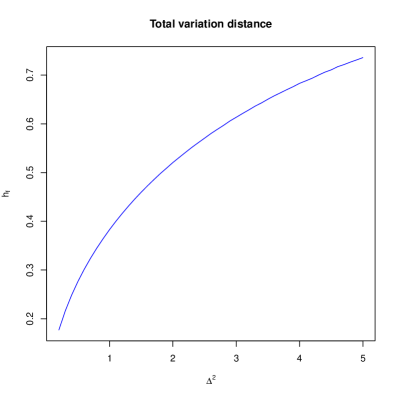
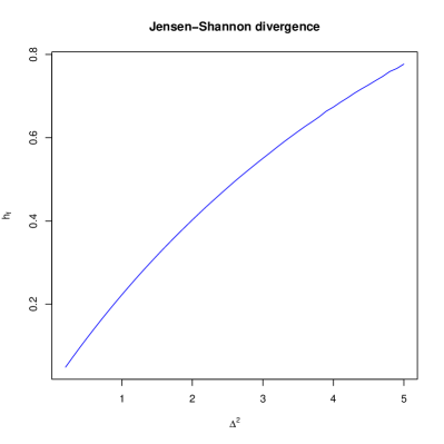
Figure 1: Estimating the functions $h_{f}(\Delta^{2})$ by Monte Carlo integration ($y$-axis is $\hat{h}_{f}(\Delta^{2})$ for $s=10^{8}$ MC samples) for the total variation distance (left) and the Jensen-Shannon divergence (right).

4 $f$-divergences in multivariate scale families

Consider the scale family $N_{\mu}=\{p_{\mu,\Sigma}\ :\ \Sigma\succ 0\}$ of $d$-variate MVNs with a prescribed location $\mu\in\mathbb{R}^{d}$. Ali and Silvey [1] proved that all $f$-divergences between any two multivariate normal distributions with prescribed mean is an increasing function of $\lvert 1-\lambda_{i}\rvert$’s, where the $\lambda_{i}$’s denote the eigenvalues of $\Sigma_{2}\Sigma_{1}^{-1}$. This property can be proven by using the definition of $f$-divergences of Eq. 1 and the fact that

$$\frac{p_{\mu,\Sigma_{2}\Sigma_{1}^{-1}}(x)}{p_{\mu,I}(x)}=\prod_{i=1}^{d}\frac{p_{0,\lambda_{i}(\Sigma_{2}\Sigma_{1}^{-1})}(x_{i})}{p_{0,1}(x_{i})}.$$

Thus we have

$$I_{f}(p_{\mu,\Sigma_{1}}:p_{\mu,\Sigma_{2}})=I_{f}\left(p_{\mu,I}:p_{\mu,\Sigma_{2}\Sigma_{1}^{-1}}\right)=E_{f}(\lvert 1-\lambda_{1}\rvert,\ldots,\lvert 1-\lambda_{d}\rvert),$$

where $E_{f}(\cdot)$ is a $d$-variate totally symmetric function (invariant to permutations of arguments). Therefore the $f$-divergences are spectral matrix divergences [13]. In particular, one interesting case is when $E_{f}(\cdot)$ is a separable function:

$$E_{f}(\lvert 1-\lambda_{1}\rvert,\ldots,\lvert 1-\lambda_{d}\rvert)=\sum_{i=1}^{d}e_{f}(\lvert 1-\lambda_{i}\rvert).$$

We shall illustrate these results with the Kullback-Leibler divergence and more generally with the $\alpha$-divergences [2] or $\alpha$-Bhattacharyya divergences [19] below:

• The Kullback-Leibler divergence: The well-known formula of the KLD between two same-mean MVNs is

  $$D_{\mathrm{KL}}(p_{\mu,\Sigma_{1}}:p_{\mu,\Sigma_{2}}) = \frac{1}{2}\left(\log\mathrm{det}(\Sigma_{2}\Sigma_{1}^{-1})+\mathrm{tr}(\Sigma_{2}\Sigma_{1}^{-1}-I)\right).$$

  This expression can be rewritten as $D_{\mathrm{KL}}(p_{\mu,\Sigma_{1}}:p_{\mu,\Sigma_{2}})=\sum_{i=1}^{d}e_{\mathrm{KL}}^{\prime}(\lambda_{i}(\Sigma_{2}\Sigma_{1}^{-1}))$ where

  $$e_{\mathrm{KL}}^{\prime}(v)=\frac{1}{2}\left(\log v+v-1\right),$$

  since $\mathrm{det}(\Sigma_{2}\Sigma_{1}^{-1})=\prod_{i=1}^{d}\lambda_{i}(\Sigma_{2}\Sigma_{1}^{-1})$ and $\mathrm{tr}(\Sigma_{2}\Sigma_{1}^{-1}-I)=\sum_{i=1}^{d}(\lambda_{i}(\Sigma_{2}\Sigma_{1}^{-1})-1)$. By a change of variable $v=1-u$, we get

  $$e_{f_{\mathrm{KL}}}(u)=\frac{1}{2}\left(\log(1-u)-u\right),$$ (4)

  and $E_{f_{\mathrm{KL}}}(u_{1},\ldots,u_{d})=\sum_{i=1}^{d}e_{f_{\mathrm{KL}}}(u_{i})$ (separable case). We check that the scalar function $e_{f_{\mathrm{KL}}}(u)$ is an increasing function of $u$.

• More generally, let us consider the family of $\alpha$-divergences [2]:

  $$D_{\alpha}(p:q)=\left\{\begin{array}[]{ll}\frac{4}{1-\alpha^{2}}\left(1-\rho_{\frac{1-\alpha}{2}}(p:q)\right),&\alpha\not\in\{-1,1\}\\ D_{\mathrm{KL}}(p:q),&\alpha=-1\\ D_{\mathrm{KL}}(q:p),&\alpha=1.\end{array}\right.,$$

  where

  $$\rho_{\beta}(p:q)=\int p^{\beta}(x)q^{1-\beta}(x)\mathrm{d}\mu(x),$$

  is the skew Bhattacharyya coefficient (a similarity measure also called an affinity measure). The skew Bhattacharyya distance [19] is $D_{\mathrm{Bhat}}(p:q)=-\log\rho_{\beta}(p:q)$. We have $D_{\alpha}(q:p)=D_{-\alpha}(p:q)$. We recover the squared Hellinger divergence when $\alpha=0$ and the Neyman $\chi^{2}$-divergence when $\alpha=3$ (and the Pearson $\chi^{2}$-divergence when $\alpha=-3$). The $\alpha$-divergences are $f$-divergences for the following family $f_{\alpha}(u)$ of generators:

  $$f_{\alpha}(u)=\left\{\begin{array}[]{ll}\frac{4}{1-\alpha^{2}}\left(u-u^{\frac{1+\alpha}{2}}\right),&\alpha\not\in\{-1,1\}\\ -\log u,&\alpha=-1\\ u\log u,&\alpha=1.\end{array}\right.$$

  We have the following closed-form formula between two scale normal distributions [23] (page 46):

  $$\rho_{\beta}(p_{\mu,\Sigma_{1}}:p_{\mu,\Sigma_{2}})=\frac{\mathrm{det}(\Sigma_{1})^{\frac{1-\beta}{2}}\,\mathrm{det}(\Sigma_{2})^{\frac{\beta}{2}}}{\mathrm{det}((1-\beta)\Sigma_{1}+\beta\Sigma_{2})^{\frac{1}{2}}}$$ (5)

  We can rewrite Eq. 5 as follows:

  $$\mathrm{det}((1-\beta)\Sigma_{1}+\beta\Sigma_{2})=\mathrm{det}(I+\beta(\Sigma_{2}\Sigma_{1}^{-1}-I))\,\mathrm{det}(\Sigma_{1}),$$

  so that

  $$\rho_{\beta}(p_{\mu,\Sigma_{1}}:p_{\mu,\Sigma_{2}})=\frac{\mathrm{det}(\Sigma_{2}\Sigma_{1}^{-1})^{\frac{\beta}{2}}}{\mathrm{det}(I+\beta(\Sigma_{2}\Sigma_{1}^{-1}-I))^{\frac{1}{2}}}.$$

  Using the eigenvalues $\lambda_{i}$’s for $i\in\{1,\ldots,d\}$ of $\Sigma_{2}\Sigma_{1}^{-1}$, we have

  $$\rho_{\beta}(p_{\mu,\Sigma_{1}}:p_{\mu,\Sigma_{2}})=\prod_{i=1}^{d}\sqrt{\frac{\lambda_{i}^{\beta}}{1+\beta(\lambda_{i}-1)}}.$$

  Indeed, consider the characteristic polynomial

  $$p_{\Sigma_{2}\Sigma_{1}^{-1}}(x)=\mathrm{det}\left(xI-\Sigma_{2}\Sigma_{1}^{-1}\right)=\prod_{i=1}^{d}(x-\lambda_{i}(\Sigma_{2}\Sigma_{1}^{-1})).$$

  We have $\mathrm{det}\left(\Sigma_{2}\Sigma_{1}^{-1}\right)=p_{\Sigma_{2}\Sigma_{1}^{-1}}(0)=(-1)^{d}\prod_{i=1}^{d}\lambda_{i}$ and

  $$\mathrm{det}\left(I+\beta(\Sigma_{2}\Sigma_{1}^{-1}-I)\right)=\beta^{d}\mathrm{det}\left(\left(\frac{1}{\beta}-1\right)\Sigma_{2}\Sigma_{1}^{-1}\right)=\beta^{d}p_{\Sigma_{2}\Sigma_{1}^{-1}}\left(\frac{1}{\beta}-1\right).$$

  Thus the $\alpha$-divergences or the Bhattacharyya divergences are increasing functions of the $\lvert 1-\lambda_{i}\rvert$’s as stated by Ali and Silvey [1].

Notice that the bounds on the total variation distance between two multivariate Gaussian distributions with same mean has been investigated in [8] but no closed-form formula is known.

Finally, we show that the $f$-divergences between two densities of a scale family are always spectral matrix divergences:

Proposition 3.

For location-scale families $\{p_{\mu,\Sigma}(x)=(\mathrm{det}\Sigma)^{-1/2}p(\Sigma^{-1/2}(x-\mu))\}_{\mu,\Sigma}$ where $p$ is the standard density such that $p(x)=\widetilde{p}(\lvert x\rvert^{2})$ for some $\widetilde{p}$, every $f$-divergence $I_{f}(p_{\mu,\Sigma_{1}}:p_{\mu,\Sigma_{2}})$ between scale family is a function of the eigenvalues of $\Sigma_{1}\Sigma_{2}^{-1}$.

Proof.

We can assume that $\mu=0$. By the change-of-variable $x=\Sigma_{1}^{1/2}y$,

$$I_{f}(p_{\mu,\Sigma_{1}}:p_{\mu,\Sigma_{2}})=\int_{\mathbb{R}^{d}}f\left(\left(\frac{\mathrm{det}\Sigma_{1}}{\mathrm{det}\Sigma_{2}}\right)^{1/2}\frac{\widetilde{p}(x^{\top}\Sigma_{2}^{-1}x)}{\widetilde{p}(x^{\top}\Sigma_{1}^{-1}x)}\right)dx$$

$$=\int_{\mathbb{R}^{d}}f\left(\left(\frac{\mathrm{det}\Sigma_{1}}{\mathrm{det}\Sigma_{2}}\right)^{1/2}\frac{\widetilde{p}\left(y^{\top}\Sigma_{1}^{1/2}\Sigma_{2}^{-1}\Sigma_{1}^{1/2}y\right)}{\widetilde{p}(\lvert y\rvert^{2})}\right)dy.$$

Since $\Sigma_{1}$ and $\Sigma_{2}$ are both symmetric matrices, $\Sigma_{1}^{1/2}$ and $\Sigma_{2}^{-1}$ are both symmetric, and hence, $\Sigma_{1}^{1/2}\Sigma_{2}^{-1}\Sigma_{1}^{1/2}$ is also symmetric. Hence it is diagonalizable by an orthogonal matrix and there exist real eigenvalues $\lambda_{1},\dots,\lambda_{d}$ and $\mathrm{det}(\Sigma_{1}^{1/2}\Sigma_{2}^{-1}\Sigma_{1}^{1/2})=\lambda_{1}\cdots\lambda_{d}$. Since $\Sigma_{2}$ is positive-definite, $\Sigma_{2}^{-1}$ is also positive-definite. By this and the fact that $\Sigma_{1}^{1/2}$ is symmetric, $\Sigma_{1}^{1/2}\Sigma_{2}^{-1}\Sigma_{1}^{1/2}$ is positive-definite, and hence, $\lambda_{1},\dots,\lambda_{d}$ are all positive. Now we recall that the set of eigenvalues of $\Sigma_{1}^{1/2}\Sigma_{2}^{-1}\Sigma_{1}^{1/2}$ is identical with the set of eigenvalues of $\Sigma_{1}^{1/2}\Sigma_{1}^{1/2}\Sigma_{2}^{-1}=\Sigma_{1}\Sigma_{2}^{-1}$, which is a well-known result in linear algebra. Hence,

$$\int_{\mathbb{R}^{d}}f\left(\left(\frac{\mathrm{det}\Sigma_{1}}{\mathrm{det}\Sigma_{2}}\right)^{1/2}\frac{\widetilde{p}\left(y^{\top}\Sigma_{1}^{1/2}\Sigma_{2}^{-1}\Sigma_{1}^{1/2}y\right)}{\widetilde{p}(\lvert y\rvert^{2})}\right)dy$$

$$=\int_{\mathbb{R}^{d}}f\left(\left(\lambda_{1}\cdots\lambda_{d}\right)^{1/2}\frac{\widetilde{p}\left(\lambda_{1}y_{1}^{2}+\cdots+\lambda_{d}y_{d}^{2}\right)}{\widetilde{p}(\lvert y\rvert^{2})}\right)dy_{1}\cdots dy_{d}.$$

∎

References

- [1] Syed Mumtaz Ali and Samuel D Silvey. A general class of coefficients of divergence of one distribution from another. Journal of the Royal Statistical Society: Series B (Methodological), 28(1):131–142, 1966.
- [2] Shun-Ichi Amari. Information Geometry and Its Applications. Applied Mathematical Sciences. Springer Japan, Tokyo, Japan, 2016.
- [3] Arindam Banerjee, Srujana Merugu, Inderjit S Dhillon, Joydeep Ghosh, and John Lafferty. Clustering with Bregman divergences. Journal of machine learning research, 6(10), 2005.
- [4] Miquel Calvo and Josep Maria Oller. An explicit solution of information geodesic equations for the multivariate normal model. Statistics & Risk Modeling, 9(1-2):119–138, 1991.
- [5] Thomas M Cover. Elements of information theory. John Wiley & Sons, Hoboken, NJ, USA, 1999.
- [6] Imre Csiszár. Eine informationstheoretische ungleichung und ihre anwendung auf beweis der ergodizitaet von markoffschen ketten. Magyer Tud. Akad. Mat. Kutato Int. Koezl., 8:85–108, 1964.
- [7] Jason Davis and Inderjit Dhillon. Differential entropic clustering of multivariate gaussians. Advances in Neural Information Processing Systems, 19, 2006.
- [8] Luc Devroye, Abbas Mehrabian, and Tommy Reddad. The total variation distance between high-dimensional Gaussians with the same mean. arXiv preprint arXiv:1810.08693, 2018.
- [9] Bent Fuglede and Flemming Topsoe. Jensen-Shannon divergence and Hilbert space embedding. In International Symposium onInformation Theory (ISIT), page 31. IEEE, 2004.
- [10] Wolfgang Globke and Raul Quiroga-Barranco. Information geometry and asymptotic geodesics on the space of normal distributions. Information Geometry, 4(1):131–153, 2021.
- [11] Mohammadali Khosravifard, Dariush Fooladivanda, and T Aaron Gulliver. Confliction of the convexity and metric properties in -divergences. IEICE Transactions on Fundamentals of Electronics, Communications and Computer Sciences, 90(9):1848–1853, 2007.
- [12] Tonu Kollo. Advanced multivariate statistics with matrices. Springer, Berlin/Heidelberg, Germany, 2005.
- [13] Brian Kulis, Mátyás A Sustik, and Inderjit S Dhillon. Low-Rank Kernel Learning with Bregman Matrix Divergences. Journal of Machine Learning Research, 10(2), 2009.
- [14] Jianhua Lin. Divergence measures based on the Shannon entropy. IEEE Transactions on Information theory, 37(1):145–151, 1991.
- [15] Prasanta Chandra Mahalanobis. On the generalized distance in statistics. Proceedings of the National Institute of Sciences (Calcutta), 2:49–55, 1936.
- [16] Joseph V Michalowicz, Jonathan M Nichols, and Frank Bucholtz. Calculation of differential entropy for a mixed Gaussian distribution. Entropy, 10(3):200–206, 2008.
- [17] Geert Molenberghs and Emmanuel Lesaffre. Non-linear integral equations to approximate bivariate densities with given marginals and dependence function. Statistica Sinica, pages 713–738, 1997.
- [18] Frank Nielsen. On information projections between multivariate elliptical and location-scale families. arXiv preprint arXiv:2101.03839, 2021.
- [19] Frank Nielsen and Sylvain Boltz. The Burbea-Rao and Bhattacharyya centroids. IEEE Transactions on Information Theory, 57(8):5455–5466, 2011.
- [20] Frank Nielsen and Richard Nock. On the chi square and higher-order chi distances for approximating -divergences. IEEE Signal Processing Letters, 21(1):10–13, 2013.
- [21] Frank Nielsen and Kazuki Okamura. On -divergences between Cauchy distributions. arXiv preprint arXiv:2101.12459, 2021.
- [22] Esa Ollila, David E Tyler, Visa Koivunen, and H Vincent Poor. Complex elliptically symmetric distributions: Survey, new results and applications. IEEE Transactions on signal processing, 60(11):5597–5625, 2012.
- [23] Leandro Pardo. Statistical inference based on divergence measures. Chapman and Hall/CRC, Boca Raton, Florida, 2018.
- [24] Mohammad H Rohban, Prakash Ishwar, Burkay Orten, William Clement Karl, and Venkatesh Saligrama. An impossibility result for high dimensional supervised learning. In 2013 IEEE Information Theory Workshop (ITW), pages 1–5. IEEE, 2013.
- [25] AGM Steerneman and F Van Perlo-Ten Kleij. Spherical distributions: Schoenberg (1938) revisited. Expositiones Mathematicae, 23(3):281–287, 2005.