Investigating $R_{D}$ and $R_{D^{*}}$ anomalies in a Left-Right model with an Inverse Seesaw

Abstract

We investigate $R_{D}$ and $R_{D^{*}}$ anomalies in a low scale left-right symmetric model based on $SU(3)_{C}\times SU(2)_{L}\times SU(2)_{R}\times U(1)_{B-L}\times Z_{2}$ with a simplified Higgs sector consisting of only one bidoublet and one $SU(2)_{R}$ doublet. The Wilson coefficients relevant to the transition $b\to c\tau\nu$ are derived by integrating out the charged Higgs $H^{\pm}$ boson, which gives the dominant contributions. We emphasize that the charged Higgs effects, with the complex right-handed quark mixing matrix, can account for both $R_{D}$ and $R_{D^{*}}$ anomalies simultaneously, while adhering to the constraints from ${\rm BR}(B^{-}_{c}\to\tau^{-}\bar{\nu}_{\tau})$.

I Introduction

In flavor physics, the two ratios $R_{D}$ and $R_{D^{*}}$ are among several long-term tensions between the Standard Model (SM) and the related experimental measurements. These ratios are defined by

$$R(\{D^{*},D\})\equiv\frac{\mathcal{B}(B_{q}\rightarrow\{D^{*},D\}\tau\nu)}{\mathcal{B}(B_{q}\rightarrow\{D^{*},D\}l\nu)}\,,$$ (1)

where $l=e,\mu$. The processes $B_{q}\rightarrow\{D^{*},D\}\ell\nu$ with $\ell=l,\tau$ arise at tree-level from the four fermion transition $b\rightarrow c\tau\nu$. Upon combining different experimental data by BaBar Collaboration Lees:2012xj ; Lees:2013uzd , Belle Collaboration Huschle:2015rga ; Hirose:2016wfn ; Hirose:2017dxl ; Belle:2019rba and LHCb Collaboration Aaij:2015yra ; Aaij:2017deq ; Aaij:2017uff , the Heavy Flavor Averaging Group (HFLAV) obtained the average of $R_{D}$ and $R_{D^{*}}$ for 2021 as HFLAV ,

$$R_{D} =0.339\pm 0.026\pm 0.014\,,$$ (2)

$$R_{D^{*}} =0.295\pm 0.010\pm 0.010\,.$$ (3)

The corresponding averages of SM predictions as reported by HFLAV HFLAV based on the predictions obtained in Refs.  Bigi:2016mdz ; Gambino:2019sif ; Bordone:2019vic are given by

$$R_{D}^{\mathrm{SM}} =0.298\pm 0.003\,,$$ (4)

$$R_{D^{*}}^{\mathrm{SM}} =0.252\pm 0.005\,.$$ (5)

Clearly, the listed results of $R_{D}$ and $R_{D^{*}}$ in Eqs.(2,3) exceed the SM predictions given above, by $1.4\sigma$ and $2.9\sigma$ respectively. Moreover, as reported by HFLAV HFLAV , the difference with the SM predictions reported above, corresponds to about $3.4\sigma[R_{D}-R_{D^{*}}]$ combination. This may serve as a hint for a violation of lepton-flavor universality.

In the literature, many theoretical models have been investigated aiming to explain the $R_{D}$ and $R_{D^{*}}$ anomalies. Based on the remark that the measured ratio $R_{D^{*}}$ is higher than its value in the SM, attempts in many models have focused on enhancing the rate of $b\to c\tau\nu$ transition through extra contributions arising from the new particles mediating the transition. This turns to be much easier than reducing the rate of $b\to c(e,\mu)\nu$ transitions, given the much more severe restraints on the couplings of new physics to muons and electrons Asadi:2018wea .

The new particles mediating the $b\to c\tau\nu$ can be spin-0 or spin-1. In addition, they can either carry baryon and lepton number (leptoquarks) or be $B/L$ neutral (charged Higgs and $W^{\prime}$). As reported in Ref. Asadi:2018wea , the existing models can be classified into three main categories :

• Models with charged Higgs Tanaka:2010se ; Fajfer:2012jt ; Crivellin:2012ye ; Celis:2012dk . In these class of models, integrating out the charged Higgs, that mediates $b\to c\tau\nu$ transition at tree-level results in scalar-scalar operators contributing to decay rates. The contributions of these additional operators can be constrained using the measured $B_{c}$ lifetime. This leads to the upper limits ${\rm BR}(B_{c}^{-}\to\tau^{-}\bar{\nu}_{\tau})\leq 40$ Celis:2016azn , ${\rm BR}(B_{c}^{-}\to\tau^{-}\bar{\nu}_{\tau})\leq 30$ Alonso:2016oyd and a much stronger bound ${\rm BR}(B_{c}^{-}\to\tau^{-}\bar{\nu}_{\tau})\leq 10\%$ was obtained from the LEP data taken at the $Z$ peak Akeroyd:2017mhr . Later on, the bounds using the measured $B_{c}$ lifetime had been critically investigated and relaxed upper limit of $\leq 39\%$ Bardhan:2019ljo and $\leq 60\%$ Blanke:2018yud ; Blanke:2019qrx were obtained.

• Models with Heavy charged vector bosons He:2012zp ; Boucenna:2016qad . In such class of models, integrating out $W^{\prime}$’s yields new contributions to the vector-vector operators. Simultaneous explanation of both $R_{D}$ and $R_{D^{*}}$ with left-handed neutrinos requires non zero values for the associated new contributions. It should be noted that, these class of models are subjected to constraints originating from the presence of an accompanying $Z^{\prime}$ mediator. Thus, the vertex $Z^{\prime}b_{L}s_{L}$ can be inferred from the $W^{\prime}b_{L}c_{L}$ vertex through the $SU(2)$ invariance. The $Z^{\prime}b_{L}s_{L}$ term in the Lagrangian can lead to tree-level flavor-changing neutral currents (FCNCs) and hence there is a need to some mechanism to subdue the contributions of this term. One way to do that is to assume minimal flavor violation (MFV) as considered in Refs. Greljo:2015mma ; Faroughy:2016osc . However, adopting this choice in general can not suppress $Z^{\prime}bb$ and $Z^{\prime}\tau\tau$ vertices. Consequently, LHC direct searches for $Z^{\prime}\to\tau\tau$ resonances can result in stringent restraints on the related parameters of the models. However, as shown in Refs. Faroughy:2016osc ; Crivellin:2017zlb , selecting unnaturally high $Z^{\prime}$ widths helps to avoid these severe constraints.

• Models with Leptoquarks Fajfer:2012jt ; Tanaka:2012nw . Either scalar and vector leptoquarks can be potentially favored as an explanations for the $R_{D^{(*)}}$ anomaly Crivellin:2017zlb ; Calibbi:2017qbu . These models are subjected also to many important constraints including those from $b\rightarrow s\nu\nu$ restraints Crivellin:2017zlb , searches at the LHC for $\tau\tau$ resonances Faroughy:2016osc ; Crivellin:2017zlb , and the measured $B_{c}$ life-time Alonso:2016oyd ; Akeroyd:2017mhr . However, these constraints turn to be weaker compared to the corresponding ones imposed on the alternative models described above Asadi:2018wea .

In this study, we aim to derive the effective Hamiltonian resulting from the four fermion transition $b\to c\tau\nu$ in the minimal left-right model with an inverse-seesaw (LRIS). At tree-level, the transition is mediated by the exchanging of the charged Higgs boson in the model. Having the effective Hamiltonian, we will proceed to show the dominant Wilson coefficients contributing to the ratios $R_{D}$ and $R_{D^{*}}$. Consequently, we will display the dependency of the ratios on the parameters of the model to determine the most relevant ones. Moreover, we reexamine the relation between the observable $R_{D^{*}}$ and ${\rm BR}(B_{c}\to\tau\bar{\nu}_{\tau})$, reported in Refs. Alonso:2016oyd ; Akeroyd:2017mhr , in light of Belle combination Belle:2019rba and LHCb Aaij:2017deq experimental results, and the projection at Belle II experiment with an integrated luminosity of 50 $\rm ab^{-1}$ Belle-II:2018jsg . This turns to be very important because the constraint on ${\rm BR}(B_{c}\to\tau\bar{\nu}_{\tau})$ affects substantially the contributions from scalar operators Bardhan:2019ljo ; Blanke:2018yud ; Blanke:2019qrx . Finally, we will also investigate the possibility of resolving the anomalies after including the new contributions to the Wilson coefficients of the total effective Hamiltonian in the presence of the LRIS model.

This paper is organized as follows. In Sec. II, we give a brief review of the Left-Right Model with inverse seesaw. In the review, we discuss the gauge structure and the particle content of the model. We also discuss the fermion interactions with charged Higgs and with the charged $W,W^{\prime}$ gauge bosons. These interactions are required to derive the effective Hamiltonian governs the processes contributing to $R_{D}$ and $R_{D^{*}}$.Then, in Sec. III, we present the effective Hamiltonian describing $b\to c\tau\nu$ transition in the presence of a general New Physics (NP) beyond the SM. Particularly, we derive the analytic expressions of the Wilson coefficients up to one loop level originating from the charged Higgs mediation in LRIS model under study in this paper. Based on the Hamiltonian, we show the total expressions of $R_{D}$ and $R_{D^{*}}$. In Sec. IV, we give our estimation of $R_{D}$ and $R_{D^{*}}$ and their dependency on the parameter space. Finally, in Sec. V, we give our conclusion.

II Left-Right Model with inverse seesaw (LRIS)

The gauge sector of the minimal left-right model with an inverse-seesaw (LRIS) is based on the symmetry $SU(3)_{C}\times SU(2)_{L}\times SU(2)_{R}\times U(1)_{B-L}$. The particle content of the model includes the usual particles in the SM in addition to extra fermions, scalars and gauge bosons. Regarding the fermion content of the model, it is the same as its counterpart in the conventional left-right models Mohapatra:1974gc ; Senjanovic:1975rk ; Mohapatra:1977mj ; Deshpande:1990ip ; Aulakh:1998nn ; Maiezza:2010ic ; Borah:2010zq ; Nemevsek:2012iq . The implementation of the IS mechanism for neutrino masses can be carried out via introducing three SM singlet fermions $S_{1}$ with $B-L$ charge $=+2$ and three singlet fermions $S_{2}$ with $B-L$ charge $=-2$. It should be remarked that, this particular choice of the $B-L$ charges of the pair $S_{1,2}$ assures that the $U(1)_{B-L}$ anomaly is free.

The scalar sector of the LRIS model contains the SM Higgs doublet, an extra new $SU(2)_{R}$ scalar doublet $\chi_{R}$ and a scalar bidoublet $\phi$. The extra doublet and bidoublet are essential for breaking the symmetries of the model upon having nonvanishing VEVs $\langle\zeta\rangle\neq 0$ for $\zeta=\phi,\chi_{R}$. We define $\langle\chi_{R}\rangle=v_{R}/\sqrt{2}$ and assume that $v_{R}$ of an order TeV to break the right-handed electroweak sector together with $B-L$. Regarding the VEV of the scalar bidoublet $\phi$, we use the parametrization $\langle\phi\rangle=\text{diag}(k_{1}/\sqrt{2},k_{2}/\sqrt{2})$ where $k_{1}=vs_{\beta},~{}k_{2}=vc_{\beta}$ and hence $v^{2}=k_{1}^{2}+k_{2}^{2}$ with $v$ of an order $\mathcal{O}(100)~{}\text{GeV}$ to break the electroweak symmetry of the SM. Here and after we use the definitions $s_{x}=\sin x,~{}c_{x}=\cos x$, $t_{x}=\tan x$ and $ct_{x}=\cot x$.

The scalar-fermion interactions in the LRIS model can be inferred from the left-right symmetric Yukawa Lagrangian which can be generally expressed as

$$\mathcal{L}_{\text{Y}}=\sum_{i,j=1}^{3}y_{ij}^{L}\bar{L}_{Li}\phi L_{Rj}+\tilde{y}_{ij}^{L}\bar{L}_{Li}\tilde{\phi}L_{Rj}+y_{ij}^{Q}\bar{Q}_{Li}\phi Q_{Rj}+\tilde{y}_{ij}^{Q}\bar{Q}_{Li}\tilde{\phi}Q_{Rj}+y^{s}_{ij}\bar{L}_{Ri}\tilde{\chi}_{R}S^{c}_{2j}+H.c.,$$ (6)

here $i$ and $j$ are family indices that run from $1\ldots 3$, $y^{Q}$ and $\tilde{y}^{Q}$ represent the quark Yukawa couplings while $y^{L}$ and $\tilde{y}^{L}$ stand for the lepton Yukawa couplings. It should be noted that a $Z_{2}$ discrete symmetry is implemented in order to forbid a mixing mass term $M\bar{S^{c}_{1}}S_{2}$ and thus preserving the IS mechanism, as discussed in Khalil:2010iu . Under this symmetry, only $S_{1}$ has an odd charge while the rest of other particles have even charges. The fields in Eq.(6) are defined as

$$\chi_{R}=\begin{pmatrix}\chi_{R}^{+}\\ \chi_{R}^{0}\\ \end{pmatrix},\,\,\,\,\phi=\begin{pmatrix}\phi_{1}^{0}&\phi_{1}^{+}\\ \phi_{2}^{-}&\phi_{2}^{0}\\ \end{pmatrix},\,\,\,\,Q_{A}=\begin{pmatrix}u_{A}\\ d_{A}\\ \end{pmatrix},\,\,\,L_{A}=\begin{pmatrix}\nu_{A}\\ e_{A}\\ \end{pmatrix},\,\,\,\,for\,\,\,A=L,R.$$ (7)

The dual bidoublet $\widetilde{\phi}$ and doublet $\widetilde{\chi}_{R}$ are defined as $\widetilde{\phi}=\tau_{2}\phi^{*}\tau_{2}$ and $\widetilde{\chi}_{R}=i\tau_{2}\chi^{*}_{R}$ respectively. Clearly, from the scalar sector of the model and before symmetry breaking, there are $12$ scalar degrees of freedom: $4$ of $\chi_{R}$ and $8$ of $\phi$. After symmetry breaking, six scalars out of these $12$ degrees of freedom remain as physical Higgs bosons while the other degrees of freedom are eaten by the neutral gauge bosons: $Z_{\mu}$ and $Z^{\prime}_{\mu}$ and the charged gauge bosons: $W^{\pm}_{\mu}$ and $W^{\prime\pm}_{\mu}$ to acquire their masses. The physical Higgs bosons are two charged Higgs bosons, one pseudoscalar Higgs boson, and the remaining three are $CP$-even neutral Higgs bosons. For a detailed discussion about the Higgs sector of the LRIS model we refer to Ref.Ezzat:2021bzs .

We turn now to the neutrino sector of LRIS model. After breaking the $B-L$ symmetry, a nonrenormalizable term of dimension seven $\propto\chi_{R}^{4}\bar{S^{c}_{2}}S_{2}/M^{3}$ yields a small mass term $\mu_{s}\bar{S^{c}_{2}}S_{2}$. In turn, this implies that $\mu_{s}=\lambda_{s}v_{R}^{4}/M^{3}\raise 1.29167pt\hbox{$\;<$\kern-7.5pt\raise-4.73611pt\hbox{$\sim\;$}}\mathcal{O}(1)~{}\text{KeV}$ Abdallah:2011ew . Here $\lambda_{s}$ stands for an interaction effective dimensionless coupling. With the adopted choice $v_{R}\sim\mathcal{O}(10^{3})~{}\text{GeV}$, one can see that $\mu_{s}\sim\mathcal{O}(10^{-7})~{}\text{GeV}$ corresponding to $\lambda_{s}/M^{3}\sim\mathcal{O}(10^{-19})~{}\text{GeV}$. For a choice $\lambda_{s}\sim\mathcal{O}(1)$, the nonrenormalizable scale $M$ is an intermediate scale, namely $M\sim\mathcal{O}(10^{3})~{}\text{TeV}$ whereas for $\lambda_{s}\sim\mathcal{O}(10^{-3})$, one obtains $M\sim\mathcal{O}(10)~{}\text{TeV}$. Consequently, the Lagrangian of neutrino masses can be expressed as

$${\cal L}_{m}^{\nu}=M_{D}\bar{\nu}_{L}\nu_{R}+M_{R}\bar{\nu}^{c}_{R}S_{2}+\mu_{s}\bar{S^{c}_{2}}S_{2}+H.c.,$$ (8)

where $M_{R}$ and $M_{D}$ are $3\times 3$ matrices related to $v_{R}$ and Dirac neutrino masses respectively via $M_{R}=y^{s}v_{R}/\sqrt{2}$ and $M_{D}=v(y^{L}s_{\beta}+\tilde{y}^{L}c_{\beta})/\sqrt{2}$ in the standard neutrino IS matrices Mohapatra:1986aw ; Mohapatra:1986bd ; GonzalezGarcia:1988rw ; Weiland:2013xia . In the flavor basis $\psi=(\nu_{L}^{c},\nu_{R},S_{2})$, we have a term $\bar{\psi}^{c}\mathcal{M}_{\nu}\psi$ where $\mathcal{M}_{\nu}$ is the $9\times 9$ neutrino mass matrix given by

$$\mathcal{M}_{\nu}=\begin{pmatrix}0&M_{D}&0\\ M_{D}^{T}&0&M_{R}\\ 0&M_{R}^{T}&\mu_{s}\end{pmatrix}.$$ (9)

Following the standard procedure, the diagonalization of $\mathcal{M}_{\nu}$ results in the light and heavy neutrino mass eigen states $\nu_{\ell_{i}},\nu_{h_{j}}$ with the mass eigenvalues given by:

$$m_{\nu_{\ell_{i}}} =M_{D}M_{R}^{-1}\mu_{s}(M_{R}^{T})^{-1}M_{D}^{T},\quad i=1\ldots 3,$$ (10)

$$m_{\nu_{h_{j}}}^{2} =M_{R}^{2}+M_{D}^{2},\quad j=1\ldots 6.$$ (11)

The light neutrino mass matrix in Eq.(10) must be diagonalized by the physical neutrino mixing matrix $U_{\!M\!N\!S}$ mns , i.e.,

$$U_{\!M\!N\!S}^{T}m_{\nu_{\ell_{i}}}U_{\!M\!N\!S}=m_{\nu_{\ell_{i}}}^{\rm d}\equiv{\rm diag}\{m_{\nu_{e}},m_{\nu_{\mu}},m_{\nu_{\tau}}\}.$$ (12)

Thus, one can easily show that the Dirac neutrino mass matrix can be defined as :

$$M_{D}=U_{\!M\!N\!S}\,\sqrt{m_{\nu_{\ell_{i}}}^{\rm d}}\,R\,\sqrt{\mu^{-1}_{s}}\,M_{R},$$ (13)

where $R$ is an arbitrary orthogonal matrix. Clearly, for $M_{R}$ at TeV scale and $\mu_{s}\ll M_{R}$ the light neutrino masses can be of order eV. The $9\times 9$ neutrino mass matrix ${\cal M}_{\nu}$, can be diagonalized with the help of the matrix $V$ satisfying $V^{T}{\cal M}_{\nu}V={\cal M}_{\nu}^{\rm diag}$. The matrix can be expressed as Dev:2009aw

$$V=\left(\begin{array}[]{cc}V_{3\times 3}&V_{3\times 6}\\ V_{6\times 3}&V_{6\times 6}\\ \end{array}\right).$$ (14)

As a good approximation, the matrix $V_{3\times 3}$ can be given a

$$V_{3\times 3}\simeq\left(1-\frac{1}{2}FF^{T}\right)U_{\!M\!N\!S}\,.$$ (15)

where $F=M_{D}M^{-1}_{R}$. Generally $F$, as one can see from the expression of $V_{3\times 3}$, is not unitary matrix. This unitarity violation, i.e., , the deviation from the standard $U_{\!M\!N\!S}$ matrix, depends on the size of $\frac{1}{2}FF^{T}$ Abdallah:2011ew . The matrix $V_{3\times 6}$ is given by

$$V_{3\times 6}=\left({\bf 0}_{3\times 3},F\right)V_{6\times 6}.$$ (16)

Finally, the matrix $V_{6\times 6}$ is the one that diagonalize the $\{\nu_{R},S_{2}\}$ mass matrix.

The process under study can receive dominant contributions from the charged Higgs mediation at tree level as we will show in the following. Thus, below, we list the relevant charged Higgs couplings related to our study following Ref.Ezzat:2021bzs . In the flavor basis $(\phi_{1}^{\pm},\phi_{2}^{\pm},\chi_{R}^{\pm})$, the charged Higgs bosons symmetric mass matrix takes the form

$$M_{H^{\pm}}^{2}=\frac{\alpha_{32}}{2}\begin{pmatrix}\frac{v_{R}^{2}s_{\beta}^{2}}{c_{2\beta}}&\frac{v_{R}^{2}s_{2\beta}}{2c_{2\beta}}&-vv_{R}s_{\beta}\\ .&\frac{v_{R}^{2}c_{\beta}^{2}}{c_{2\beta}}&-vv_{R}c_{\beta}\\ .&.&v^{2}c_{2\beta}\end{pmatrix}.$$ (17)

The above matrix can be diagonalized by the unitary matrix,

$$Z^{H^{\pm}}=\begin{pmatrix}\frac{vc_{2\beta}}{\sqrt{v^{2}c_{2\beta}^{2}+v_{R}^{2}s_{\beta}^{2}}}&0&\frac{v_{R}s_{\beta}}{\sqrt{v^{2}c_{2\beta}^{2}+v_{R}^{2}s_{\beta}^{2}}}\\ -\frac{\frac{1}{2}v_{R}^{2}s_{2\beta}}{\sqrt{(v^{2}c_{2\beta}^{2}+v_{R}^{2}s_{\beta}^{2})(v^{2}c_{2\beta}^{2}+v_{R}^{2})}}&\sqrt{\frac{v^{2}c_{2\beta}^{2}+v_{R}^{2}s_{\beta}^{2}}{v^{2}c_{2\beta}^{2}+v_{R}^{2}}}&\frac{vv_{R}c_{\beta}c_{2\beta}}{\sqrt{(v^{2}c_{2\beta}^{2}+v_{R}^{2}s_{\beta}^{2})(v^{2}c_{2\beta}^{2}+v_{R}^{2})}}\\ -\frac{v_{R}s_{\beta}}{\sqrt{v^{2}c_{2\beta}^{2}+v_{R}^{2}}}&-\frac{v_{R}c_{\beta}}{\sqrt{v^{2}c_{2\beta}^{2}+v_{R}^{2}}}&\frac{vc_{2\beta}}{\sqrt{v^{2}c_{2\beta}^{2}+v_{R}^{2}}}\end{pmatrix}.$$ (18)

The mass eigenstates basis can be obtained using the rotation $(\phi_{1}^{\pm},\phi_{2}^{\pm},\chi_{R}^{\pm})^{T}=Z^{H^{\pm}T}(G_{1}^{\pm},G_{2}^{\pm},H^{\pm})^{T}$ such that $Z^{H^{\pm}}M_{H^{\pm}}^{2}Z^{H^{\pm}T}=\text{diag}(0,0,m_{H^{\pm}}^{2})$. Here $G_{1}^{\pm}$ and $G_{2}^{\pm}$ represent the massless charged Goldstone bosons and $H^{\pm}$ is a massive physical charged Higgs boson. The massless Goldstone bosons are eaten by the charged gauge bosons $W_{\mu}$ and $W^{\prime}_{\mu}$ to acquire their masses via the familiar Higgs mechanism. On the other hand, the mass of the charged Higgs boson $H^{\pm}$ is given by:

$$m_{H^{\pm}}^{2}=\frac{\alpha_{32}}{2}\left(\frac{v_{R}^{2}}{c_{2\beta}}+v^{2}c_{2\beta}\right),$$ (19)

where $\alpha_{32}=\alpha_{3}-\alpha_{2}$. Clearly, the charged Higgs boson mass can be of the order of hundreds GeV if we pick out the values $v_{R}\sim\mathcal{O}(\text{TeV})$ and $\alpha_{32}\sim\mathcal{O}(10^{-2})$. It is clear to see that, the physical charged Higgs boson is a linear combination of the flavor basis fields $\phi_{1}^{\pm},\phi_{2}^{\pm},\chi_{R}^{\pm}$, namely given as

$$H^{\pm}=Z^{H^{\pm}}_{13}\phi_{1}^{\pm}+Z^{H^{\pm}}_{23}\phi_{2}^{\pm}+Z^{H^{\pm}}_{33}\chi_{R}^{\pm}.$$ (20)

The effective Lagrangian, in the LRIS model, describing the charged Higgs and the charged gauge bosons $W$ and $W^{\prime}$ couplings to quarks and leptons can be expressed as

$$\mathcal{L}_{eff}=\mathcal{L}^{\bar{q}q^{\prime}H^{\pm}}_{eff}+\mathcal{L}^{\bar{\nu}\ell H^{\pm}}_{eff}+\mathcal{L}^{W,W^{\prime}}_{eff}$$ (21)

The Lagrangians $\mathcal{L}^{\bar{q}q^{\prime}H^{\pm}}_{eff}$ and $\mathcal{L}^{\bar{\nu}\ell H^{\pm}}_{eff}$ can be obtained from expanding $\mathcal{L}_{\text{Y}}$, given in Eq.(6), and rotating the fields to their corresponding ones in the mass eigenstates basis. It is direct to obtain

$$\mathcal{L}^{\bar{q}q^{\prime}H^{\pm}}_{eff} = \bar{u}_{i}{\Gamma_{u_{i}d_{j}}^{H^{\pm}\,LR\,\rm{eff}}}P_{R}d_{j}H^{\pm}\,+\bar{u}_{i}{\Gamma_{u_{i}d_{j}}^{H^{\pm}\,RL\,\rm{eff}}}P_{L}d_{j}H^{\pm}+h.c.\,,$$ (22)

where

$${\Gamma_{u_{i}d_{j}}^{H^{\pm}\,LR\,\rm{eff}}} = \sum_{a=1}^{3}(V^{R}_{CKM})^{*}_{ja}y^{Q}_{ia}Z_{{32}}^{H^{\pm}}+\sum_{a=1}^{3}(V^{R}_{CKM})^{*}_{ja}\tilde{y}^{Q}_{ia}Z_{{31}}^{H^{\pm}}$$

$${\Gamma_{u_{i}d_{j}}^{H^{\pm}\,RL\,\rm{eff}}} = \sum_{a=1}^{3}(V^{L}_{CKM})^{*}_{ja}y^{Q^{*}}_{ai}Z_{{31}}^{H^{\pm}}+\sum_{a=1}^{3}(V^{L}_{CKM})^{*}_{ja}\tilde{y}^{Q^{*}}_{ai}Z_{{32}}^{H^{\pm}}.$$ (23)

In the LRIS model and after electroweak symmetry breaking, quarks and charged leptons acquire their masses via Higgs mechanism. Consequently, we can express the quark Yukawa couplings in terms of the quark masses and CKM matrices in the left and right sectors as

$$y^{Q} = \frac{1}{(t_{\beta}-ct_{\beta})}\bigg{(}\frac{M^{diag}_{u}V_{\text{CKM}}^{R{\dagger}}}{v_{d}}-\frac{V^{L}_{\text{CKM}}M^{diag}_{d}}{v_{u}}\bigg{)}$$

$$\tilde{y}^{Q} = \frac{1}{(ct_{\beta}-t_{\beta})}\bigg{(}\frac{M^{diag}_{u}V_{\text{CKM}}^{R{\dagger}}}{v_{u}}-\frac{V^{L}_{\text{CKM}}M^{diag}_{d}}{v_{d}}\bigg{)},$$ (24)

with $v=246$ GeV, $v_{u}=\frac{vs_{\beta}}{\sqrt{2}}$, $v_{d}=\frac{vc_{\beta}}{\sqrt{2}}$. In the above equation, $M^{diag}_{u}(M^{diag}_{d})$ is the diagonal up (down) quark mass matrix, $V^{L}_{\text{CKM}}$ and $V^{R}_{\text{CKM}}$ are the CKM matrices in the left and right sectors respectively. The mixing matrices for left and right quarks result in the CKM matrices in the left and right sectors $V_{\text{CKM}}^{L,R}=V^{u{\dagger}}_{L,R}V^{d}_{L,R}$. We can choose the bases where $V^{u}_{L}=I$ and as a result, in this basis, $V_{\text{CKM}}^{L}=V^{d}_{L}$. Turning now to the right sector, we follow Ref.Kiers:2002cz , where the matrix $V^{R}_{\text{CKM}}$ is given by

$$V^{R}_{\text{CKM}}=K~{}V^{L}_{\text{CKM}}\left(\theta^{R}_{12},\theta^{R}_{23},\theta^{R}_{13},\delta_{R}\right)~{}\tilde{K}^{+},$$ (25)

here the diagonal matrices $K$ and $\tilde{K}$ contain five of six non-removable phases in $V^{R}_{\text{CKM}}$. It was emphasized that CP violation and FCNC in the right-handed sector can be under control if the $V^{R}_{\text{CKM}}$ is of the form

$$V^{R}_{\text{CKM}}=\left(\begin{array}[]{ccc}1&0&0\\ 0&c_{\theta^{R}_{13}}&s_{\theta^{R}_{13}}e^{i\alpha}\\ 0&s_{\theta^{R}_{13}}&-c_{\theta^{R}_{13}}e^{i\alpha}\end{array}\right),$$ (26)

where $c_{\theta^{R}_{13}}=\cos(\theta^{R}_{13})$ and $s_{\theta^{R}_{13}}=\sin(\theta^{R}_{13})$ and as we will see that, in the following, the phase $\alpha$ in the third column plays an important role in increasing the values of $R_{D^{*}}$. It is also possible to have a non-vanishing phase in the second column, which turns out to be irrelevant and has no effect on the $R_{D}$ or $R_{D^{*}}$ results. Therefore, we set it to zero. We work in the bases where $V^{d}_{R}=I$ and thus $V_{\text{CKM}}^{R}=V^{u}_{R}$, similar to the left-handed quark sector.

We proceed now to the lepton-neutrinio charged Higgs interactions in the model under study. These interactions contribute to the effective Lagrangian $\mathcal{L}^{\bar{\nu}\ell H^{\pm}}_{eff}$ and generally, can be written as

$$\mathcal{L}^{\bar{\nu}\ell H^{\pm}}_{eff} = \bar{\nu}_{i}{\Gamma_{\nu_{i}\ell_{j}}^{H^{\pm}\,LR\,\rm{eff}}}P_{R}\ell_{j}H^{\pm}\,+\bar{\nu}_{i}{\Gamma_{\nu_{i}\ell_{j}}^{H^{\pm}\,RL\,\rm{eff}}}P_{L}\ell_{j}H^{\pm}+h.c.\,,$$ (27)

with

$${\Gamma_{\nu_{i}\ell_{j}}^{H^{\pm}\,LR\,\rm{eff}}} = \sum_{a=1}^{3}\tilde{y}^{L}_{aj}V_{{ia}}Z_{{31}}^{H^{\pm}}-\sum_{a=1}^{3}y^{L}_{aj}V_{{ia}}Z_{{32}}^{H^{\pm}}-\sum_{a=1}^{3}y^{s*}_{ja}V_{{i6+a}}Z_{{33}}^{H^{\pm}}$$

$${\Gamma_{\nu_{i}\ell_{j}}^{H^{\pm}\,RL\,\rm{eff}}} = -\sum_{a=1}^{3}V^{*}_{{i3+a}}y^{L*}_{ja}Z_{{31}}^{H^{\pm}}+\sum_{a=1}^{3}V^{*}_{{i3+a}}\tilde{y}^{L*}_{ja}Z_{{32}}^{H^{\pm}}.$$ (28)

The lepton Yukawa couplings $y^{L}$ and $\tilde{y}^{L}$ can be expressed as

$$y^{L} =\frac{t_{2\beta}}{\sqrt{2}\,v_{u}}\bigg{(}M_{\ell}-t_{\beta}M_{D}\bigg{)}\,,$$ (29)

$$\tilde{y}^{L} =\frac{t_{2\beta}}{\sqrt{2}\,v_{u}}\bigg{(}M_{D}-t_{\beta}M_{\ell}\bigg{)},$$ (30)

where $M_{\ell}$ is charged lepton diagonal mass matrix. Finally, the leptons and quarks gauge interactions related to our processes at tree-level can be deduced from the effective Lagrangian $\mathcal{L}^{W,W^{\prime}}_{eff}$ given by

$$\mathcal{L}^{W,W^{\prime}}_{eff} = \frac{1}{\sqrt{2}}g_{2}\cos\phi_{W}(V_{\text{CKM}}^{L})^{*}_{ji}W_{\mu}\bar{u}_{i}\gamma_{\mu}P_{L}d_{j}-\frac{1}{\sqrt{2}}g_{R}\sin\phi_{W}(V_{\text{CKM}}^{R})^{*}_{ji}W_{\mu}\bar{u}_{i}\gamma_{\mu}P_{R}d_{j}$$ (31)

$$+ \frac{1}{\sqrt{2}}g_{2}\sin\phi_{W}(V_{\text{CKM}}^{L})^{*}_{ji}W^{\prime}_{\mu}\bar{u}_{i}\gamma_{\mu}P_{L}d_{j}-\frac{1}{\sqrt{2}}g_{R}\cos\phi_{W}(V_{\text{CKM}}^{R})^{*}_{ji}W^{\prime}_{\mu}\bar{u}_{i}\gamma_{\mu}P_{R}d_{j}$$

$$+ \frac{1}{\sqrt{2}}g_{2}\cos\phi_{W}V_{{ij}}W_{\mu}\bar{\nu}_{i}\gamma_{\mu}P_{L}e_{j}-\frac{1}{\sqrt{2}}g_{R}\sin\phi_{W}V^{*}_{{i3+j}}W_{\mu}\bar{\nu}_{i}\gamma_{\mu}P_{R}e_{j}$$

$$+ \frac{1}{\sqrt{2}}g_{2}\sin\phi_{W}V_{{ij}}W^{\prime}_{\mu}\bar{\nu}_{i}\gamma_{\mu}P_{L}e_{j}-\frac{1}{\sqrt{2}}g_{R}\cos\phi_{W}V^{*}_{{i3+j}}W^{\prime}_{\mu}\bar{\nu}_{i}\gamma_{\mu}P_{R}e_{j}+h.c.\,,$$

where $\phi_{W}$ is the mixing angle between $W_{L}$ and $W_{R}$, which is of order $10^{-3}$. We have now all the ingredient required for deriving the effective Hamiltonian contributing to the transition $b\to c\tau\nu$. In next section, we derive this Hamiltonian and list the expressions of the Wilson coefficients corresponding to this Hamiltonian.

III The effective Hamiltonian relevant to the processes in the LRIS

In the presence of NP beyond SM, the effective Hamiltonian governs $|\Delta c|=1$ B decays transition relevant to our processes up to one-loop level derived from the diagrams in Fig.1, can be expressed as

$${\mathcal{H}}_{eff} = -\frac{4G_{F}}{\sqrt{2}}V_{cb}\bigg{(}(1+g_{V}^{LL})\,(\bar{c}\gamma_{\mu}P_{L}b)(\bar{\ell}_{j}\gamma^{\mu}P_{L}\nu_{i})+g_{V}^{RR}(\bar{c}\gamma_{\mu}P_{R}b)(\bar{\ell}_{j}\gamma^{\mu}P_{R}\nu_{i})+g_{V}^{LR}(\bar{c}\gamma_{\mu}P_{L}b)(\bar{\ell}_{j}\gamma^{\mu}P_{R}\nu_{i})$$ (32)

$$+ g_{V}^{RL}(\bar{c}\gamma_{\mu}P_{R}b)(\bar{\ell}_{j}\gamma^{\mu}P_{L}\nu_{i})+g_{S}^{LL}(\bar{c}P_{L}b)(\bar{\ell}_{j}P_{L}\nu_{i})+g_{S}^{RR}(\bar{c}P_{R}b)(\bar{\ell}_{j}P_{R}\nu_{i})+g_{S}^{LR}(\bar{c}P_{L}b)(\bar{\ell}_{j}P_{R}\nu_{i})$$

$$+ g_{S}^{RL}(\bar{c}P_{R}b)(\bar{\ell}_{j}P_{L}\nu_{i})+g_{T}^{LL}(\bar{c}\sigma_{\mu\nu}P_{L}b)(\bar{\ell}_{j}\sigma^{\mu\nu}P_{L}{\nu}_{i})+g_{T}^{RR}(\bar{c}\sigma_{\mu\nu}P_{R}b)(\bar{\ell}_{j}\sigma^{\mu\nu}P_{R}{\nu}_{i})\bigg{)},$$

where $V_{cb}$ is the $cb$ Cabibbo-Kobayashi-Maskawa (CKM) matrix element, $P_{L,R}=\frac{1}{2}(1\mp\gamma_{5})$, $\sigma_{\mu\nu}=\frac{i}{2}[\gamma_{\mu},\gamma_{\nu}]$ and as mentioned in Ref.Tanaka:2012nw the tensor operator with chirality $(\bar{c}\sigma_{\mu\nu}P_{R}b)(\bar{\ell}_{j}\sigma^{\mu\nu}P_{L}{\nu}_{i})$ vanishes. In case of $\ell=\tau$ we find that

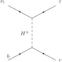
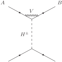
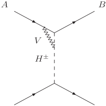
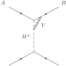
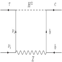
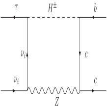
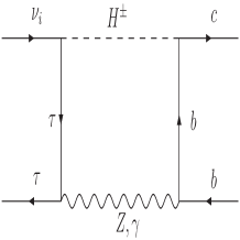
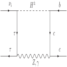
Figure 1: Diagrams contributing to ${\mathcal{H}}_{eff}$, in Eq.(32) up to one loop-level due to charged Higgs mediation with $V=Z,\gamma$.

$$g_{V}^{LL} = (\cos^{2}\phi_{W}+\frac{m^{2}_{W}}{m^{2}_{W^{\prime}}}\sin^{2}\phi_{W})Z_{M,{i3}}^{v},$$

$$g_{V}^{RR} = \frac{1}{V_{cb}}(\sin^{2}\phi_{W}+\frac{m^{2}_{W}}{m^{2}_{W^{\prime}}}\cos^{2}\phi_{W})(V_{\text{CKM}}^{R})^{*}_{32}Z^{v,*}_{M,{i6}},$$

$$g_{V}^{LR} = -(1+\frac{m^{2}_{W}}{m^{2}_{W^{\prime}}})Z^{v,*}_{M,{i6}}\cos\phi_{W}\sin\phi_{W},$$

$$g_{V}^{RL} = -\frac{1}{V_{cb}}(1+\frac{m^{2}_{W}}{m^{2}_{W^{\prime}}})(V_{\text{CKM}}^{R})^{*}_{32}Z_{M,{i3}}^{v}\cos\phi_{W}\sin\phi_{W},$$

$$g_{S}^{LL} = -\frac{\sqrt{2}}{4G_{F}V_{cb}m^{2}_{H^{\pm}}}{\Gamma_{u_{2}d_{3}}^{H^{\pm}\,RL\,\rm{eff}}}{(\Gamma_{\nu_{i}\ell_{3}}^{H^{\pm}\,LR\,\rm{eff}})^{*}},$$

$$g_{S}^{RR} = -\frac{\sqrt{2}}{4G_{F}V_{cb}m^{2}_{H^{\pm}}}{\Gamma_{u_{2}d_{3}}^{H^{\pm}\,LR\,\rm{eff}}}{(\Gamma_{\nu_{i}\ell_{3}}^{H^{\pm}\,RL\,\rm{eff}})^{*}},$$

$$g_{S}^{LR} = -\frac{\sqrt{2}}{4G_{F}V_{cb}m^{2}_{H^{\pm}}}{\Gamma_{u_{2}d_{3}}^{H^{\pm}\,RL\,\rm{eff}}}{(\Gamma_{\nu_{i}\ell_{3}}^{H^{\pm}\,RL\,\rm{eff}})^{*}},$$

$$g_{S}^{RL} = -\frac{\sqrt{2}}{4G_{F}V_{cb}m^{2}_{H^{\pm}}}{\Gamma_{u_{2}d_{3}}^{H^{\pm}\,LR\,\rm{eff}}}{(\Gamma_{\nu_{i}\ell_{3}}^{H^{\pm}\,LR\,\rm{eff}})^{*}},$$

$$g_{T}^{LL} = -\frac{\sqrt{2}\alpha_{E}}{96\pi G_{F}V_{cb}m^{2}_{H^{\pm}}}{\Gamma_{u_{2}d_{3}}^{H^{\pm}\,RL\,\rm{eff}}}{(\Gamma_{\nu_{i}\ell_{3}}^{H^{\pm}\,LR\,\rm{eff}})^{*}}\bigg{(}f(x_{c},x_{\tau})+\frac{1}{2}f(x_{b},x_{\tau})\bigg{)}+\Delta g^{LL\,Z,Z^{\prime}}_{{T}},$$

$$g_{T}^{RR} = -\frac{\sqrt{2}\alpha_{E}}{96\pi G_{F}V_{cb}m^{2}_{H^{\pm}}}{\Gamma_{u_{2}d_{3}}^{H^{\pm}\,LR\,\rm{eff}}}{(\Gamma_{\nu_{i}\ell_{3}}^{H^{\pm}\,RL\,\rm{eff}})^{*}}\bigg{(}f(x_{c},x_{\tau})+\frac{1}{2}f(x_{b},x_{\tau})\bigg{)}+\Delta g^{RR\,Z,Z^{\prime}}_{T},$$ (33)

where $i$ refers to the neutrino flavor, $x_{k}=\frac{m_{k}^{2}}{m^{2}_{H}}$ and $f(x_{i},x_{j})=\frac{1}{(x_{i}-x_{j})}\Big{(}\frac{x_{i}}{1-x_{i}}logx_{i}-(x_{i}\leftrightarrow x_{j})\Big{)}$.

As can be seen from Eq.(33), the coefficients $g_{S}^{LL}$ and $g_{S}^{RL}$ have the same lepton vertex $(\Gamma_{\nu_{i}\ell_{3}}^{H^{\pm}\,LR\,\rm{eff}})^{*}$. Therefore, they are expected to have different values due to receiving different contributions of the quark vertices $\Gamma_{u_{i}d_{j}}^{H^{\pm}\,RL\,\rm{eff}}$ and $\Gamma_{u_{i}d_{j}}^{H^{\pm}\,LR\,\rm{eff}}$ expressed in Eq.(23) in terms of $y^{Q}$ and $\tilde{y}^{Q}$. Furthermore, Eq.(24) shows that the contributions from the terms proportional to $V^{L}_{CKM}$ to both $y^{Q}$ and $\tilde{y}^{Q}$ are suppressed by the small down quark masses appear in the matrix $M^{diag}_{d}$.

In the processes under consideration, the corresponding Wilson coefficient $g_{S}^{LL}$ ($g_{S}^{RL}$) receives contributions only from the elements in the second column (row) of the matrix $M^{diag}_{u}V_{\text{CKM}}^{R{\dagger}}$, which are present in both of $y^{Q}$ and $\tilde{y}^{Q}$. With the texture of $V_{\text{CKM}}^{R}$ given previously, we find that

$$M^{diag}_{u}V_{\text{CKM}}^{R{\dagger}}=\left(\begin{array}[]{ccc}m_{u}&0&0\\ 0&m_{c}\,c_{\theta^{R}_{13}}&m_{c}\,s_{\theta^{R}_{13}}\\ 0&m_{t}\,s_{\theta^{R}_{13}}e^{-i\alpha}&m_{t}\,c_{\theta^{R}_{13}}e^{-i\alpha}\\ \end{array}\right).$$ (34)

In this regard, one can show that $R_{D}$, $R_{D^{*}}$ and ${\rm BR}(B^{-}_{c}\to\tau^{-}\bar{\nu}_{\tau})$ receive contributions from the terms proportional to $m_{t}\,s_{\theta^{R}_{13}}e^{-i\alpha}$ which originate from $g_{S}^{LL}$ only and not from $g_{S}^{RL}$. The other contributions generated from the Wilson coefficient $g_{S}^{RL}$ are proportional to the charm quark mass which is small compared to the top quark mass.

Finally in Eq.(33), the quantities $\Delta g^{LL(RR)\,Z,Z^{\prime}}_{T}$ refer to the suppressed contributions, comparing to photon ones, originating from $Z$ and $Z^{\prime}$ mediating the diagrams. Upon neglecting the small contributions $\Delta g^{LL,RR\,Z,Z^{\prime}}_{T}$ we find the following relations

$g_{T}^{LL}=-\frac{\alpha_{E}}{24\pi}\bigg{(}f(x_{c},x_{\tau})+\frac{1}{2}f(x_{b},x_{\tau})\bigg{)}g_{S}^{LL}$ and $g_{T}^{RR}=-\frac{\alpha_{E}}{24\pi}\bigg{(}f(x_{c},x_{\tau})+\frac{1}{2}f(x_{b},x_{\tau})\bigg{)}g_{S}^{RR}$. For a charged Higgs of a mass $430\,GeV$ we find that $g_{T}^{LL}\simeq 1.5\times 10^{-3}g_{S}^{LL}$ and $g_{T}^{RR}\simeq 1.5\times 10^{-3}g_{S}^{RR}$. Clearly the tensor contributions to the processes under study can be safely neglected.

We will assume that NP effects are only present in the third generation of leptons ($\tau,\nu_{\tau}$). This assumption is motivated by the absence of deviations from the SM for light lepton modes $\ell=e$ or $\mu$. The ratios $R(M)$ ($M=D,D^{\ast}$ can be written in terms of the scalar $g_{S}^{LL},g_{S}^{RL},C_{S}^{LR},$ and $C_{S}^{RR}$ Iguro:2018vqb ; Asadi:2018wea ; Asadi:2018sym . The numerical expressions for these contributions are Iguro:2018vqb ; Asadi:2018wea ; Asadi:2018sym :

$$R_{D} = R_{D}^{\rm SM}\Big{[}1+1.49\ \text{Re}(g_{S}^{RL}+g_{S}^{LL})^{\ast}+1.02\big{(}|g_{S}^{RL}+g_{S}^{LL}|^{2}+|g_{S}^{LR}+g_{S}^{RR}|^{2}\big{)}\Big{]},$$ (35)

$$R_{D^{*}} = R_{D^{*}}^{\rm SM}\Big{[}1+0.11\ \text{Re}(g_{S}^{RL}-g_{S}^{LL})^{\ast}+0.04\big{(}|g_{S}^{RL}-g_{S}^{LL}|^{2}+|g_{S}^{LR}-g_{S}^{RR}|^{2}\big{)}\Big{]}.$$ (36)

The tree-level charged Higgs boson exchange also modifies the branching ratio of the tauonic decay $B_{c}^{-}\to\tau^{-}\bar{\nu}_{\tau}$ as follows Iguro:2018vqb ; Asadi:2018wea ; Asadi:2018sym

$${\rm BR}(B_{c}^{-}\to\tau^{-}\bar{\nu}_{\tau}) = {\rm BR}(B_{c}^{-}\to\tau^{-}\bar{\nu}_{\tau})_{\text{SM}}\ \left[\bigg{|}1+\frac{m_{B_{c}}^{2}}{m_{\tau}(m_{b}+m_{c})}(g_{S}^{RL}-g_{S}^{LL})\bigg{|}^{2}+\bigg{|}\frac{m_{B_{c}}^{2}}{m_{\tau}(m_{b}+m_{c})}(g_{S}^{LR}-g_{S}^{RR})\bigg{|}^{2}\right],$$

where $m_{B_{c}}^{2}/m_{\tau}(m_{b}+m_{c})=4.065$ and

$${\rm BR}(B^{-}_{c}\to\tau^{-}\bar{\nu}_{\tau})_{\rm SM} = \tau_{B_{c}}\dfrac{G_{F}^{2}}{8\pi}|V_{cb}|^{2}f_{B_{c}}^{2}m_{B_{c}}m_{\tau}^{2}\Big{(}1-\dfrac{m_{\tau}^{2}}{m_{B_{c}}^{2}}\Big{)}^{2},$$ (38)

where $V_{cb}$ stands for the CKM matrix element, $\tau_{B_{c}}$ and $f_{B_{c}}$ denote the $B^{-}_{c}$ meson lifetime and decay constant, respectively. The SM prediction of ${\rm BR}(B^{-}_{c}\to\tau^{-}\bar{\nu}_{\tau})_{\rm SM}=(2.25\pm 0.21)\times 10^{-2}$ Fleischer:2021yjo . Unfortunately, no direct constraints from upper bounds on the leptonic $B_{c}$ branching ratios are available from the LHC. In view of this, an estimate of a bound on ${\rm BR}(B^{-}_{c}\to\tau^{-}\bar{\nu}_{\tau})$ has been derived from LEP data at the Z peak in Ref. Akeroyd:2017mhr . The bound turns to be strong ${\rm BR}(B_{c}^{-}\to\tau^{-}\bar{\nu}_{\tau})\leq 10\%$. Later on, the bounds using the measured $B_{c}$ lifetime had been critically investigated and relaxed upper limit of $\leq 39\%$ Bardhan:2019ljo and $\leq 60\%$ Blanke:2018yud ; Blanke:2019qrx were obtained. Thus we will follow Ref. Fleischer:2021yjo and take in our analysis the bound: ${\rm BR}(B^{-}_{c}\to\tau^{-}\bar{\nu}_{\tau})<60\%$

IV Numerical results and analysis

It is worth to recall that, due to the requirement of having light neutrino masses we found that the contributions of the right neutrino sector to the the corresponding Wilson coefficients $g_{S}^{RR}$ and $g_{S}^{LR}$ are very small and thus can be safely ignored, leaving us with only $g_{S}^{LL}$ and $g_{S}^{RL}$. Furthermore, $g_{S}^{RL}$ is about one order of magnitude smaller than $g_{S}^{LL}$; thus for real $g_{S}^{LL}$ and $g_{S}^{RL}$ (i.e., $Re(g_{S}^{AB})=g_{S}^{AB}$), one finds

$$R_{D} \simeq R_{D}^{\rm SM}\Big{[}1+1.49g_{S}^{LL}+1.02|g_{S}^{LL}|^{2}\Big{]},$$ (39)

$$R_{D^{*}} \simeq R_{D^{*}}^{\rm SM}\Big{[}1-0.11g_{S}^{LL}+0.04|g_{S}^{LL}|^{2}\Big{]}.$$ (40)

This expression clearly shows that enhancing the values of $R_{D^{*}}$ to be in the range of the given experimental results, while keeping the limit $-1\raise 1.29167pt\hbox{$\;<$\kern-7.5pt\raise-4.73611pt\hbox{$\sim\;$}}g_{S}^{LL}\raise 1.29167pt\hbox{$\;<$\kern-7.5pt\raise-4.73611pt\hbox{$\sim\;$}}1$ in mind is possible for a range of negative values of $g_{S}^{LL}$ as can be seen from the left plot in Fig.2. However, as can be remarked from the right plot in Fig.2, these negative values reduce $R_{D}$ below their allowed $2\sigma$ range of the experimental results shown by the horizontal orange and blue lines in the plot. Clearly, we deduce that the phase $\alpha$ of the mixing matrix $V^{R}_{CKM}$ is crucial to solve the concerned anomalies for the processes under consideration.

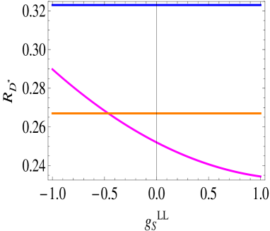
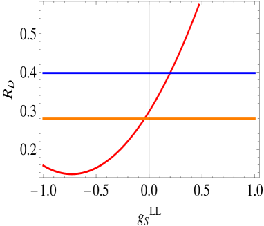
Figure 2: Left (right) $R_{D^{*}}$ ($R_{D}$) variation with $g_{S}^{LL}$ where the horizontal orange and blue lines represent the allowed $2\sigma$ range of their experimental values.

The attainable values of the Wilson coefficients $g_{S}^{LL}$ and $g_{S}^{RL}$ are affected by the charged Higgs mass. As a result, to enhance these coefficients and thus the values of $R_{D}$ and $R_{D^{*}}$ while adhering to direct search constraints, the charged Higgs masses should not be too heavy, namely of the order of hundreds GeV. According to Eq.(19), this can be accomplished by considering $v_{R}\sim\mathcal{O}(\text{TeV})$, $\alpha_{32}\sim\mathcal{O}(10^{-2})$ and $t_{\beta}$ less than one. Remarkably, from the pre factor $1/(t_{\beta}-ct_{\beta})$ in Eq.(24), it is direct to see that small $t_{\beta}$ values can enhance also the quark Yukawa couplings and hence together with the angle $\theta^{R}_{13}$ and the complex phase $\alpha$ of the right-quark mixing $V^{R}_{CKM}$, defined in Eq.(26), play crucial roles in increasing the values of $R_{D}$ and $R_{D^{*}}$, and allow them to take values that are compatible with the limit of the experiments at the same time. In our scan of the parameter space we take $\alpha_{32}\in[0.007,0.016]$, $t_{\beta}\in[0.15,0.25]$, $c_{\theta^{R}_{13}}\in[-1,1]$, $\alpha\in[0,\pi]$ and $v_{R}=6413$ GeV. With this in hand, we show below our results corresponding to the scanned points in the parameter space respecting the bound ${\rm BR}(B^{-}_{c}\to\tau^{-}\bar{\nu}_{\tau})<60\%$. Moreover, we have checked that, for these parameters in the chosen ranges and values, the contribution of the $g_{S}^{RL}$ are irrelevant and can be safely neglected. This confirms our previous conclusion that only the Wilson coefficient $g_{S}^{LL}$ plays the major role through the terms proportional to $m_{t}\,s_{\theta^{R}_{13}}e^{-i\alpha}$. In the following, we present a set of elucidative plots of $R_{D}$ and $R_{D^{*}}$ versus some selected relevant parameters of the model.

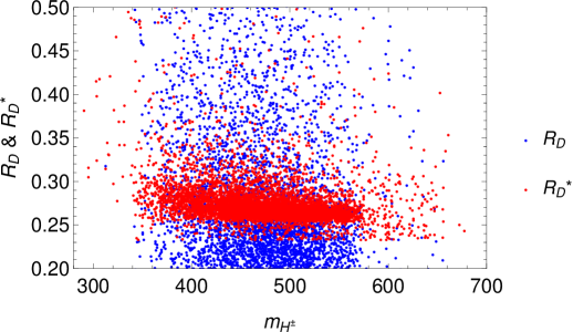
Figure 3: $R_{D}$ and $R_{D^{*}}$ as function of the charged Higgs mass where the parameters as stated in the text are chosen as follows: $c_{\theta^{R}_{13}}\in[-1,1]$, $\alpha\in[0,\pi]$, $\alpha_{32}\in[0.007,0.016]$ and $t_{\beta}\in[0.15,0.25]$.

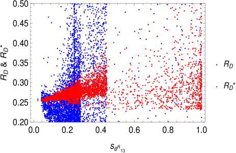
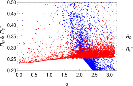
Figure 4: $R_{D}$ and $R_{D^{*}}$ as function of the sin of mixing angle $\theta^{R}_{13}$ left and the phase $\alpha$ of the $V^{R}_{CKM}$ matrix right and other parameters are fixed as in the previous figure. In the left plot we show the points corresponding to $\theta^{R}_{13}\in[0,\frac{\pi}{2}]$ as $\theta^{R}_{13}$ close to zero are favored for resolving the $R_{D}$ and $R_{D^{*}}$ anomalies.

In Fig. 3, we display the variation of $R_{D}$ and $R_{D^{*}}$ with the charged Higgs mass. As can be seen from the figure, it is possible to account for the experimental results of $R_{D}$ and $R_{D^{*}}$ within $2\sigma$ range while respecting the ${\rm BR}(B^{-}_{c}\to\tau^{-}\bar{\nu}_{\tau})$ constraints with charged Higgs masses $m_{H^{\pm}}$ can be chosen of order 500 GeV. On the other hand, the dependence of $R_{D}$ and $R_{D^{*}}$ on the sin of the mixing angle $\theta^{R}_{13}$ and the phase $\alpha$ of the $V^{R}_{CKM}$ matrix is depicted in Fig. 4. It is clear from left plot in the figure that, small values of $s_{\theta^{R}_{13}}$ are preferable to satisfy the experimental results of $R_{D}$ and $R_{D^{*}}$ within $2\sigma$ range while respecting the ${\rm BR}(B^{-}_{c}\to\tau^{-}\bar{\nu}_{\tau})$ constraints. However, this is not the case regarding the phase $\alpha$ as in this case large phases are favored as can be seen from the right plot in the figure.

We can obtain the regions in the $(\theta^{R}_{13},\alpha)$ parameter space in which the anomalies are satisfied through varying $\theta^{R}_{13}$ and $\alpha$ while assigning fixed values of the other parameters. As an example, we take the fixed values $t_{\beta}\simeq 0.21$, $\alpha_{32}=0.015$ which result in $m_{H^{\pm}}=580$ GeV and the other parameters are fixed as before. In Fig.5 left, we show the experimentally allowed $2\sigma$ regions in the $(\theta^{R}_{13},\alpha)$ plane of $R_{D^{*}}$ in blue and $R_{D}$ in red without imposing the constraints from ${\rm BR}(B^{-}_{c}\to\tau^{-}\bar{\nu}_{\tau})<60\%$. As shown in the plot, the regions in which the $R_{D^{*}}$ and $R_{D}$ anomalies are satisfied correspond to values of $\theta^{R}_{13}\in[1.9,\pi]$ and approximately $\alpha\in[0.35.0.9]$ or $\alpha\in[2.2.2.8]$. However, not all these ranges of $\theta^{R}_{13}$ and $\alpha$ survive if we impose the ${\rm BR}(B^{-}_{c}\to\tau^{-}\bar{\nu}_{\tau})<60\%$ constraint which is represented in yellow color in the right plot of Fig.5. In this case, the allowed ranges are $\theta^{R}_{13}\in[1.9.2.4]$ and approximately $\alpha\in[0.35.0.55]$ or $\alpha\in[2.6.2.8]$ as can be noted from the plot. Clearly, the ${\rm BR}(B^{-}_{c}\to\tau^{-}\bar{\nu}_{\tau})$ constraint has a sensible effect on the parameter space satisfying the anomalies.

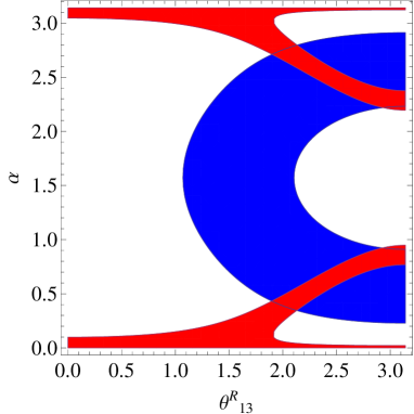
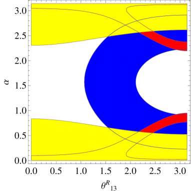
Figure 5: Left (right) the allowed regions in the ($(\theta^{R}_{13},\alpha)$) plane by the $2\sigma$ experimental results of $R_{D^{*}}$ in blue and $R_{D}$ in red without (with) imposing the constraints from ${\rm BR}(B^{-}_{c}\to\tau^{-}\bar{\nu}_{\tau})<60\%$ which is given in yellow color in the right plot for $m_{H^{\pm}}=580$ GeV for $t_{\beta}\simeq 0.21$, $\alpha_{32}=0.015$ which result in $m_{H^{\pm}}=580$ GeV and the other parameters are fixed as before.

Finally we present in Fig. 6 the correlation between $R_{D}$ and $R_{D^{*}}$ for the same set of the parameter space considered in the scan over the values and ranges mentioned in the beginning of this section. Only points that satisfy the ${\rm BR}(B^{-}_{c}\to\tau^{-}\bar{\nu}_{\tau})$ constraints are included here. It is remarkable from this figure that both $R_{D}$ and $R_{D^{*}}$ are satisfied for a larger region of parameter space, thanks to the complex mixing of right-handed quarks.

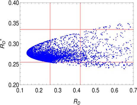
Figure 6: The correlation between $R_{D}$ and $R_{D^{*}}$ for the same set of parameter space considered in Fig. 3.

V Conclusion

In this work we have explored the possibility of resolving the tension between the SM prediction and the experimental results of the $R_{D}$ and $R_{D^{*}}$ ratios using a low scale left-right symmetric model based on $SU(3)_{C}\times SU(2)_{L}\times SU(2)_{R}\times U(1)_{B-L}\times Z_{2}$. The scalar sector of the model contains charged Higgs boson with masses that can be chosen in the order of hundreds GeV without any conflict with direct search constraints. We have shown that integrating out the charged Higgs mediating the tree-level diagrams generates a set of non vanishing scalar Wilson coefficients contributing to the effective Hamiltonian governing the transition $b\to c\tau\bar{\nu}$ and hence to the ratios $R_{D^{*}}$ and $R_{D}$.

The dependency of the scalar Wilson coefficients on the matrix elements of the quark mixing angle in the right sector turns to be important. We emphasized that the mixing element $(V^{R}_{CKM})_{23}$ should be complex in order to satisfy both $R_{D}$ and $R_{D^{*}}$. We have also shown the complex phase associated with this mixing element is essential to accommodate the experimental results of the ratios for charged Higgs masses of order 500 GeV while respecting the constraints from ${\rm BR}(B^{-}_{c}\to\tau^{-}\bar{\nu}_{\tau})$.

References

(1)
J. P. Lees et al. [BaBar Collaboration],
Evidence for an excess of decays,
Phys. Rev. Lett. 109, 101802 (2012)
[arXiv:1205.5442 [hep-ex]].
(2)
J. P. Lees et al. [BaBar Collaboration],
Measurement of an Excess of Decays and Implications for Charged Higgs Bosons,
Phys. Rev. D 88, no. 7, 072012 (2013)
[arXiv:1303.0571 [hep-ex]].
(3)
M. Huschle et al. [Belle Collaboration],
Measurement of the branching ratio of relative to decays with hadronic tagging at Belle,
Phys. Rev. D 92, no. 7, 072014 (2015)
[arXiv:1507.03233 [hep-ex]].
(4)
S. Hirose et al. [Belle Collaboration],
Measurement of the lepton polarization and in the decay ,
Phys. Rev. Lett. 118, no. 21, 211801 (2017)
[arXiv:1612.00529 [hep-ex]].
(5)
S. Hirose et al. [Belle Collaboration],
Measurement of the lepton polarization and in the decay with one-prong hadronic decays at Belle,
Phys. Rev. D 97, no. 1, 012004 (2018)
[arXiv:1709.00129 [hep-ex]].
(6)
G. Caria et al. [Belle],
Phys. Rev. Lett. 124, no.16, 161803 (2020)
doi:10.1103/PhysRevLett.124.161803 [arXiv:1910.05864 [hep-ex]].
(7)
R. Aaij et al. [LHCb Collaboration],
Measurement of the ratio of branching fractions ,
Phys. Rev. Lett. 115, no. 11, 111803 (2015)
Erratum: [Phys. Rev. Lett. 115, no. 15, 159901 (2015)]
[arXiv:1506.08614 [hep-ex]].
(8)
R. Aaij et al. [LHCb Collaboration],
Test of Lepton Flavor Universality by the measurement of the branching fraction using three-prong decays,
Phys. Rev. D 97, no. 7, 072013 (2018)
[arXiv:1711.02505 [hep-ex]].
(9)
R. Aaij et al. [LHCb Collaboration],
Measurement of the ratio of the and branching fractions using three-prong -lepton decays,
Phys. Rev. Lett. 120, no. 17, 171802 (2018)
[arXiv:1708.08856 [hep-ex]].
(10)
The updated averages of the HFLAV semileptonic group for the 2021 average,
https://hflav-eos.web.cern.ch/hflav-eos/semi/spring21/html/RDsDsstar/RDRDs.html
(12)
P. Gambino, M. Jung and S. Schacht, The puzzle: An
update, Phys. Lett. B 795, 386-390 (2019)
[arXiv:1905.08209 [hep-ph]].
(13)
M. Bordone, M. Jung and D. van Dyk,
Eur. Phys. J. C 80, no.2, 74 (2020)
doi:10.1140/epjc/s10052-020-7616-4 [arXiv:1908.09398 [hep-ph]].
(14)
P. Asadi, M. R. Buckley and D. Shih,
JHEP 09, 010 (2018) doi:10.1007/JHEP09(2018)010
[arXiv:1804.04135 [hep-ph]].
(15)
M. Tanaka and R. Watanabe,
Phys. Rev. D 82, 034027 (2010)
doi:10.1103/PhysRevD.82.034027 [arXiv:1005.4306 [hep-ph]].
(16)
S. Fajfer, J. F. Kamenik, I. Nisandzic and J. Zupan,
Phys. Rev. Lett. 109, 161801 (2012)
doi:10.1103/PhysRevLett.109.161801 [arXiv:1206.1872 [hep-ph]].
(17)
A. Crivellin, C. Greub and A. Kokulu,
Phys. Rev. D 86, 054014 (2012)
doi:10.1103/PhysRevD.86.054014 [arXiv:1206.2634 [hep-ph]].
(18)
A. Celis, M. Jung, X. Q. Li and A. Pich,
JHEP 01, 054 (2013) doi:10.1007/JHEP01(2013)054
[arXiv:1210.8443 [hep-ph]].
(19)
X. Q. Li, Y. D. Yang and X. Zhang,
JHEP 08, 054 (2016) doi:10.1007/JHEP08(2016)054
[arXiv:1605.09308 [hep-ph]].
(20)
A. Celis, M. Jung, X. Q. Li and A. Pich,
Phys. Lett. B 771, 168-179 (2017)
doi:10.1016/j.physletb.2017.05.037 [arXiv:1612.07757 [hep-ph]].
(21)
R. Alonso, B. Grinstein and J. Martin Camalich,
Phys. Rev. Lett. 118, no.8, 081802 (2017)
doi:10.1103/PhysRevLett.118.081802 [arXiv:1611.06676 [hep-ph]].
(22)
A. G. Akeroyd and C. H. Chen,
Phys. Rev. D 96, no.7, 075011 (2017)
doi:10.1103/PhysRevD.96.075011 [arXiv:1708.04072 [hep-ph]].
(23)
X. G. He and G. Valencia,
Phys. Rev. D 87, no.1, 014014 (2013)
doi:10.1103/PhysRevD.87.014014 [arXiv:1211.0348 [hep-ph]].
(24)
S. M. Boucenna, A. Celis, J. Fuentes-Martin, A. Vicente and
J. Virto,
JHEP 12, 059 (2016) doi:10.1007/JHEP12(2016)059
[arXiv:1608.01349 [hep-ph]].
(25)
A. Greljo, G. Isidori and D. Marzocca,
JHEP 07, 142 (2015) doi:10.1007/JHEP07(2015)142
[arXiv:1506.01705 [hep-ph]].
(26)
D. A. Faroughy, A. Greljo and J. F. Kamenik,
Phys. Lett. B 764, 126-134 (2017)
doi:10.1016/j.physletb.2016.11.011 [arXiv:1609.07138 [hep-ph]].
(27)
A. Crivellin, D. Müller and T. Ota,
JHEP 09, 040 (2017) doi:10.1007/JHEP09(2017)040
[arXiv:1703.09226 [hep-ph]].
(28)
M. Tanaka and R. Watanabe,
Phys. Rev. D 87, no.3, 034028 (2013)
doi:10.1103/PhysRevD.87.034028 [arXiv:1212.1878 [hep-ph]].
(29)
L. Calibbi, A. Crivellin and T. Li,
Phys. Rev. D 98, no.11, 115002 (2018)
doi:10.1103/PhysRevD.98.115002 [arXiv:1709.00692 [hep-ph]].
(30)
E. Kou et al. [Belle-II],
PTEP 2019, no.12, 123C01 (2019) [erratum: PTEP
2020, no.2, 029201 (2020)] doi:10.1093/ptep/ptz106
[arXiv:1808.10567 [hep-ex]].
(31)
D. Bardhan and D. Ghosh,
Phys. Rev. D 100, no.1, 011701 (2019)
doi:10.1103/PhysRevD.100.011701 [arXiv:1904.10432 [hep-ph]].
(32)
M. Blanke, A. Crivellin, S. de Boer, T. Kitahara, M. Moscati,
U. Nierste and I. Nišandžić,
Phys. Rev. D 99, no.7, 075006 (2019)
doi:10.1103/PhysRevD.99.075006 [arXiv:1811.09603 [hep-ph]].
(33)
M. Blanke, A. Crivellin, T. Kitahara, M. Moscati, U. Nierste and
I. Nišandžić,
doi:10.1103/PhysRevD.100.035035 [arXiv:1905.08253 [hep-ph]].
(34)
R. N. Mohapatra and J. C. Pati,
Phys. Rev. D 11, 2558 (1975) doi:10.1103/PhysRevD.11.2558
(35)
G. Senjanovic and R. N. Mohapatra,
Phys. Rev. D 12, 1502 (1975) doi:10.1103/PhysRevD.12.1502
(36)
R. N. Mohapatra, F. E. Paige and D. P. Sidhu,
Phys. Rev. D 17, 2462 (1978) doi:10.1103/PhysRevD.17.2462
(37)
N. G. Deshpande, J. F. Gunion, B. Kayser and F. I. Olness,
Phys. Rev. D 44, 837-858 (1991)
doi:10.1103/PhysRevD.44.837
(38)
C. S. Aulakh, A. Melfo and G. Senjanovic,
Phys. Rev. D 57, 4174-4178 (1998)
doi:10.1103/PhysRevD.57.4174 [arXiv:hep-ph/9707256 [hep-ph]].
(39)
A. Maiezza, M. Nemevsek, F. Nesti and G. Senjanovic,
Phys. Rev. D 82, 055022 (2010)
doi:10.1103/PhysRevD.82.055022
[arXiv:1005.5160 [hep-ph]].
(40)
D. Borah, S. Patra and U. Sarkar,
Phys. Rev. D 83, 035007 (2011)
doi:10.1103/PhysRevD.83.035007 [arXiv:1006.2245 [hep-ph]].
(41)
M. Nemevsek, G. Senjanovic and V. Tello,
Phys. Rev. Lett. 110, no.15, 151802 (2013)
doi:10.1103/PhysRevLett.110.151802 [arXiv:1211.2837 [hep-ph]].
(42)
S. Khalil,
Phys. Rev. D 82, 077702 (2010).
(43)
K. Ezzat, M. Ashry and S. Khalil,
Phys. Rev. D 104, no.1, 015016 (2021)
doi:10.1103/PhysRevD.104.015016 [arXiv:2101.08255 [hep-ph]].
(44)
W. Abdallah, A. Awad, S. Khalil and H. Okada,
Eur. Phys. J. C 72, 2108 (2012)
doi:10.1140/epjc/s10052-012-2108-9 [arXiv:1105.1047 [hep-ph]].
(45)
R. N. Mohapatra,
Phys. Rev. Lett. 56, 561-563 (1986)
doi:10.1103/PhysRevLett.56.561
(46)
R. N. Mohapatra and J. W. F. Valle,
Phys. Rev. D 34, 1642 (1986) doi:10.1103/PhysRevD.34.1642
(47)
M. C. Gonzalez-Garcia and J. W. F. Valle,
Phys. Lett. B 216, 360 (1989).
(48)
C. Weiland,
J. Phys. Conf. Ser. 447, 012037 (2013)
doi:10.1088/1742-6596/447/1/012037 [arXiv:1302.7260 [hep-ph]].
(49)
Z. Maki, M. Nakagawa and S. Sakata,
Prog. Theor. Phys. 28, 870 (1962).
(50)
P. S. B. Dev and R. N. Mohapatra,
Phys. Rev. D 81, 013001 (2010)
[arXiv:0910.3924 [hep-ph]].
(51)
K. Kiers, J. Kolb, J. Lee, A. Soni and G. H. Wu,
Phys. Rev. D 66, 095002 (2002)
doi:10.1103/PhysRevD.66.095002 [arXiv:hep-ph/0205082 [hep-ph]].
(52)
S. Iguro, T. Kitahara, Y. Omura, R. Watanabe and K. Yamamoto,
JHEP 02, 194 (2019) doi:10.1007/JHEP02(2019)194
[arXiv:1811.08899 [hep-ph]].
(53)
P. Asadi, M. R. Buckley and D. Shih,
Phys. Rev. D 99, no.3, 035015 (2019)
doi:10.1103/PhysRevD.99.035015 [arXiv:1810.06597 [hep-ph]].
(54)
R. Fleischer, R. Jaarsma and G. Tetlalmatzi-Xolocotzi,
Eur. Phys. J. C 81, no.7, 658 (2021)
doi:10.1140/epjc/s10052-021-09419-8 [arXiv:2104.04023 [hep-ph]].