Evaluating the jet/accretion coupling of Aql X-1: probing the contribution of accretion flow spectral components

Abstract

The coupling between radio and X-ray luminosity is an important diagnostic tool to study the connection between the accretion inflow and jet outflow for low-mass X-ray binaries (LMXBs). The radio/X-ray correlation for individual neutron star (NS) LMXBs is scattered, whereas for individual black hole (BH) LMXBs a more consistent correlation is generally found. Furthermore, jet quenching is observed for both types of LMXBs, but it is unclear whether jets in NS-LMXBs quench as strongly as those in BH-LMXBs. While additional soft X-ray spectral components can be detected in NS-LMXB spectra due to the presence of the neutron star’s surface, disentangling the individual X-ray spectral components has thus far not been considered when studying the radio/X-ray coupling. Here we present eleven epochs of Swift/XRT observations matched with quasi-simultaneous archival radio observations of the 2009 November outburst of Aql X-1. We decompose the thermal and Comptonised spectral components in the Swift/XRT spectra, with the aim of studying whether the presence of additional thermal emission affects the coupling of the radio/X-ray luminosity. We find that there is no evidence of a significant thermal contribution in Swift/XRT spectra that could cause scatter in the radio/X-ray coupling. To explore the role of potential spectral degeneracies in the X-ray models and consider the improvements from including hard X-rays, we perform joint fits with quasi-simultaneous RXTE/PCA spectra. Follow-up research using more sensitive, broad-band X-ray observations and densely-sampled near-simultaneous radio observations is required to study this in more detail.

1 Introduction

Coordinated, multi-wavelength observations of low mass X-ray binaries (LMXBs) allow one to probe the connection between the inflow and outflow for stellar-mass compact objects. LMXBs consist of a neutron star (NS) or a black hole (BH) and a < 1 M_⊙ companion star. In almost all LMXBs, material from the companion star is accreted onto the compact object through Roche-Lobe overflow. The material is transferred through the inner Lagrange point and forms an accretion disc around the compact object (Paczynski, 1971). Most systems show episodes of active accretion, which are proposed to be caused by instabilities in the disc (Shakura & Sunyaev, 1973; Cannizzo, 1993; Hameury et al., 2000; Lasota, 2001), alternated by quiescent periods. These episodes, or outbursts, are characterised by an increase in luminosity across the electromagnetic spectrum, driven by the increased mass accretion rate. The accretion flow emits photons from the infrared to the X-ray band, and jet outflows dominate in the radio band.

For the X-ray emission specifically, one identifies several spectral components. Firstly, the disc emits a thermal or soft component, as material in the disc is heated up during outburst. Secondly, a population of hot electrons, also often referred to as the corona, close to the compact object Compton up-scatters this thermal emission from the disc, emitting a Comptonised component. Lastly, up-scattered photons interact with the accretion disc, resulting in reflection components (Done et al., 2007; Gilfanov, 2010). These are the components that are identified in the spectra of both BH and NS-LMXBs. For NS-LMXBs, one expects to find additional spectral components. This concerns emission from the neutron star surface, and/or from the ‘boundary layer’. This boundary layer is a result of the rotating material in the accretion disc reaching the neutron star surface and decelerating (Sibgatullin & Sunyaev, 1998; Babkovskaia et al., 2008). Both of these components can be identified in soft X-ray emission, typically below 3 keV.

During outbursts of LMXBs, the ratio between the soft and hard spectral components varies over time, as the outburst progresses. Based on this ratio, combined with the timing properties of the X-ray binary, different accretion states can be distinguished. In the hard state, the Comptonised component is more prominent, while in the soft state, the thermal component is stronger (Fender et al., 2004; Done et al., 2007). The physical processes which underpin these states, and the evolution which probe the transitions, are still being debated. The transition from the hard to the soft state is often interpreted as a change in the inner-disc radius, as well as a weakening of the hot electron cloud (Done et al., 2007; Gilfanov, 2010).

Moreover, for NS-LMXBs, there is also debate on the appropriate X-ray spectral models to describe the spectra of different subtypes and/or spectral states. Some studies find degeneracies between thermal model component(s) and the Comptonised component when fitting spectra from both the hard and soft state (Lin et al., 2007). This currently presents different pictures of the structure and energetics of NS-LMXBs, further complicating the interpretation of the physical processes in these systems. Such issues may be exacerbated in X-ray observations of short exposure, limited bandpass and/or low flux, where such model degeneracies provide statistically equivalent descriptions of the data.

Classifying the spectral and timing properties of different LMXBs, allows one to track and study the transition between the hard, soft, and quiescent states. For BH-LMXBs, the evolution typically follows an increase in intensity from quiescence to the hard state, followed by a transition to the soft state through intermediate states at a somewhat constant intensity. Then the intensity decreases and the system transitions to the hard state and finally decays back to quiescence. In a hardness-intensity diagram (like presented in Fender et al., 2004), this follows a q-shape. For NS-LMXBs, the spectral behaviour is more complex. This behaviour can be identified both by the hardness-intensity diagram and the colour-colour diagram. For high accretion rates Z-shapes can be identified, and for lower accretion rates atoll-shapes can be identified in colour-colour diagrams. Comparing this to the properties of BH-LMXBs, the states identified for both these types of sources can be broadly interpreted as the equivalent of the hard, transitional/intermediate, and soft states respectively (Homan et al., 2010), and will be referred to as such in this work. During an outburst of a NS-LMXB, it will transition through these states, and often show hysteresis in the hardness-intensity diagram (Maccarone & Coppi, 2003).

When LMXB systems transition through the accretion states in the X-ray emission, one observes an evolution in the outflows seen for the radio emission as well. For BH-LMXBs, Fender et al. (2004) propose a model describing the coupling between the accretion and ejection (radio/X-ray coupling), where compact jets are observed in the hard state (Gallo et al., 2018). When the source transitions to the soft state, the radio emission of the compact jet is observed to quench (Hjellming & Wade, 1971; Harmon et al., 1995; Fender et al., 1999, 2004; Russell et al., 2011) and discrete ejecta are observed (Russell et al., 2019; Bright et al., 2020; Carotenuto et al., 2021a). For NS-LMXBs the inflow/outflow coupling is less well understood (Fender & Muñoz-Darias, 2016). Compact jets are observed during the hard state. Strongly reduced radio emission is also observed in some atoll NS-LMXBs (see e.g. Migliari et al., 2011; Miller-Jones et al., 2010; Gusinskaia et al., 2017; Díaz Trigo et al., 2018; Van den Eijnden et al., 2021), although other such systems do not appear to show clear quenching of the compact jets, remaining radio-bright following the transition to the soft state (see e.g. Migliari et al., 2003, 2004; Russell et al., 2021). It is currently unclear why only a subset of NS-LMXBs appear to show radio quenching.

To derive this inflow/outflow coupling in the hard state, one may use the correlation measured between the X-ray and radio luminosity (Hannikainen et al., 1998; Corbel et al., 2000; Corbel et al., 2003). One finds that the radio/X-ray luminosity relation for LMXBs often follow a power law relation $L_{\mathrm{R}}\propto L_{\mathrm{X}}^{\beta}$ (Corbel et al., 2002; Migliari & Fender, 2006) and that overall, when considering all sources for BH- and NS-LMXBs, both groups show approximately consistent power law slopes at the 2.5$\sigma$ level (Gallo et al., 2018). However, when considering individual sources in the BH- and NS-LMXB sample, the correlation is often more scattered (Gallo et al., 2018) with sources showing significant deviations from the general population (Carotenuto et al., 2021b) and sources showing different behaviours over different outbursts (Gusinskaia et al., 2020). Moreover, additional challenges are introduced when analysing NS-LMXB sources. These systems are systematically more faint in radio for the radio/X-ray luminosity relation, by $\approx$ 22 for similar values for the X-ray luminosity (Gallo et al., 2018). Therefore, it is more difficult to constrain the coupling between the radio and X-ray emission for individual sources, as most sources become undetectable at radio wavelengths for current observatories once their accretion rate decreases below $\sim 1$% of the Eddington luminosity.

1.1 Relation between jet and X-ray spectral components

For radio/X-ray coupling studies, the X-ray flux is typically obtained for the entire X-ray spectrum of each observation. Typically a simple absorbed power-law model is used to fit spectra of LMXB sources. However, more individual spectral components can be identified in the X-ray emission, which are shown to evolve during transitions in spectral states when LMXBs undergo outbursts. Currently, there is no decomposition of these different spectral components in analysing the radio/X-ray coupling for NS-LMXBs. The flux and luminosity for these individual spectral components could cause scatter for the coupling seen for individual systems, as these probe specific processes in the accretion flow morphology and spectral state of the system. Especially, NS-LMXBs show additional spectral components from the NS surface and/or the boundary layer as elaborated earlier. These components are not present in the spectra of BH-LMXBs, and might cause discrepancies when comparing the radio/X-ray coupling derived for both groups.

A promising source for studying individual spectral components of a NS-LMXB system, is the source Aquila X-1 (Aql X-1) because it exhibits frequent outbursts. This system is one of the first Galactic X-ray sources to be discovered (Friedman et al., 1967; Kunte et al., 1973). It is a transient LMXB (orbital period $\approx$ 19 hours, Chevalier & Ilovaisky, 1991) at a distance $d$ of around 4.5 kpc (Galloway et al., 2008). It consists of a NS (Koyama et al., 1981) and a low-mass K-type companion star (Thorstensen et al., 1978; Chevalier et al., 1999). The source is classified as an atoll source (Reig et al., 2000), and goes into outburst roughly every year (Campana et al., 2013; Güngör et al., 2017). Therefore, it is used for many studies on the radio/X-ray coupling.

Miller-Jones et al. (2010) analysed the disc-jet coupling for the 2009 outburst of Aql X-1 by triggering an observation campaign with the Karl G. Jansky Very Large Array (VLA), the Very Long Baseline Array (VLBA) and the European Very Long Baseline Interferometry Network (EVN) at 4.8 and 8.4 GHz. The X-ray data were obtained with the RXTE satellite, using the PCA (2-16 keV) and ASM (2-10 keV) count rates, as well as the count rates obtained by Swift/BAT (15-150 keV). Miller-Jones et al. (2010) found that the radio emission is consistent with being triggered during the state transition, and confirms radio quenching at X-ray luminosities of around 10 percent of the Eddington luminosity (for a 1.4 M_⊙ NS accretor this is around $L_{\mathrm{X}}\approx 10^{37}(d/5\text{kpc})^{2}$) erg/s at a distance $d$). The radio emission shows interesting behaviour during this outburst, this is discussed in more detail in Section 4. However, the analysis by Miller-Jones et al. (2010) used X-ray count rates and colors, measured above 2 keV, to study the X-ray/radio coupling. A full X-ray spectral analysis focusing on this outburst, including especially the soft X-rays, has not yet been performed. Interestingly, Swift/XRT observed this outburst and measured the X-ray spectra in the soft X-ray band (0.5-10 keV). These observations were performed in a similar time span to the radio observations, and can therefore be used to perform a radio/X-ray luminosity study.

In this paper, we use archival Swift/XRT data of the 2009 outburst of Aql X-1 to perform a detailed analysis on the X-ray spectral components. We obtain the X-ray emission and luminosity from these separate components after performing a careful consideration of the presence of the thermal component. We then use these measurements to constrain the thermal flux and its evolution during the outburst. We further evaluate the implications of model degeneracies by comparing our results with joint fits including data from RXTE. Furthermore, we use archival VLA and VLBA data from Miller-Jones et al. (2010) to analyse the radio/X-ray connection for this outburst. Using the X-ray flux obtained for the different spectral components, we evaluate the individual radio/X-ray coupling obtained for each, specifically investigating whether the presence of additional thermal emission in this NS-LMXB causes scatter in the X-ray/radio luminosity coupling. In Section 2 we present the observations and data analysis, in Section 3 the results, and we will discuss this work in Section 4.

2 Observations and Analysis

The Proportional Counter Array (PCA; Jahoda et al., 1996) onboard the RXTE satellite observed rising flux from Aql X-1 on November 1st, 2009 during an ongoing Galaxy bulge monitoring program (Markwardt et al., 2000). This rise in flux triggered multiple observing campaigns to monitor the outburst, among which the Swift telescope (Swift; Gehrels et al., 2004), the VLA and the VLBA.

The VLA and VLBA monitoring is presented by Miller-Jones et al. (2010). The outburst was observed at an observing frequency of 8.4 GHz for both observatories. More information on the calibration and reduction of the data can be found in the original paper. In this work we will use the VLA and VLBA radio flux densities reported by Miller-Jones et al. (2010) close in time to the Swift observations discussed below. We will also discuss the selection method later in this Section. The dates and radio flux densities for these observations are listed in Table 1.

Using Swift’s X-Ray Telescope (XRT) the outburst was observed within an energy range from 0.5 to 10 keV. Sixteen observations were taken in total. The first fifteen observations were obtained in Windowed Timing mode (WT) and the last observation was obtained in both WT and Photon Counting (PC) mode. We obtain the data from the Swift-XRT data products generator (Evans et al., 2007, 2009). We then fit the spectra using XSPEC (v12.11.0; Arnaud, 1996). We set the abundances and cross-sections based on Wilms et al. (2000) and Verner et al. (1996), respectively. To determine the goodness-of-fit and to estimate the best-fit spectral parameters we used the $\chi^{2}$ statistic. We also obtain the Swift/BAT (15-50 keV) light curve (Krimm et al., 2013) to illustrate the evolution of the 2009 outburst and to study the hard X-ray colour, we discuss this in Section 3. Finally, we include data from the RXTE/PCA instrument to assess potential model degeneracies. For this purpose, we download the standard-2 data products, including source and background spectra, for the RXTE observations presented in (Miller-Jones et al., 2010) and taken during the outburst phase observed by Swift. We apply the above approach to the PCA spectral analysis, and additionally include systematic errors of $0.8\%$ for PCA channels 0-39 and $2\%$ for channels 40-128 (Kreykenbohm et al., 2004; Jahoda et al., 1996). We also use the associated background spectra to determine the energy range to fit the source spectrum, corresponding to 2.6-23 keV.

Our research aims to distinguish the contribution of a black body component, probing the thermal emission of the accretion disc, neutron star surface and/or the boundary layer, and of the component induced by Comptonisation probing the corona. Therefore we used corresponding components in the model (diskbb and nthcomp, respectively), as well as a component (tbabs) to account for the absorption by the interstellar medium. The complete model is tbabs*(diskbb+nthcomp) in XSPEC syntax, and will be referred to as the composite model. We used an absorbed power-law model as well, tbabs*nthcomp, to test the significance of using a model containing a black body component. This model will be referred to as the Comptonised model. We determine the significance of the presence of a thermal component using ftest to calculate the F-statistic and its probability. Furthermore, we used cflux to calculate the flux of the total model, the diskbb component and the nthcomp component.

We only calculate the flux of the diskbb for observations where the composite model was statistically preferred over the Comptonised model. If the thermal component is not significantly present in the spectrum, we instead aimed to determine an upper limit of its flux to compare with the radio luminosity at that time. For this purpose, we used steppar to manually vary the flux parameter in the tbabs*(cflux*bbody + powerlaw) model (i.e. where the flux is only measured over the thermal component). The steppar task gradually increases the flux, at each step fixing it and subsequently fitting all other parameters, before saving the new fit statistic. Repeating this procedure for increasing fluxes, we determined the thermal flux where the fit statistic increased (i.e. worsened) by $\Delta\chi^{2}$ = 9, corresponding to 3$\sigma$ when varying a single parameter. We show an example in Figure 1, using observation X7 (see Table 1). In this Figure, the improvement in fit statistic at the best-fit diskbb flux, compared to the plateau in $\chi^{2}$ at a flux of zero (i.e. towards the right), is less than three sigma.

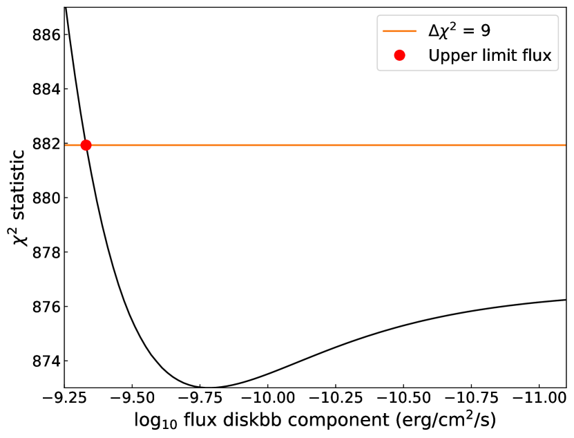
Figure 1: An example of using the steppar command to determine the 3$\sigma$ upper limit of the flux for the diskbb component for observation X7. We use steppar to manually vary the parameter around the best fitting value for the flux, i.e. where the $\chi^{2}$ statistic has the lowest value. We determine the 3$\sigma$ upper limit value where the $\chi^{2}$ statistic increased by $\Delta\chi^{2}$ = 9. The parameter value of the log₁₀ flux is shown in black, the line where $\Delta\chi^{2}$ = 9 as opposed to the minimum value for the $\chi^{2}$ statistic is shown in orange, and the obtained value for the 3$\sigma$ upper limit is indicated with a red dot.

We note that the flux in a black body spectrum scales with both normalisation (linearly) and temperature (to the fourth power), creating a parameter degeneracy; therefore, using the steppar approach on either of those parameters individually does not directly yield a flux upper limit. With the steppar approach, the best fitting combination of temperature and normalisation is found for the considered total flux in each step.

In order to determine the absorption column $n_{\mathrm{H}}$, we fit the Comptonised model to all spectra simultaneously with the tbabs parameter tied. The best fit was found for a value of $n_{\mathrm{H}}=0.355\times 10^{22}$ cm^-2 for the equivalent hydrogen column. As this is consistent with the value for $n_{\mathrm{H}}$ found in other studies (see e.g. Sakurai et al., 2012), we use this value for our analysis.

When fitting the Comptonised and composite model to the Swift/XRT spectra, we froze the value for $n_{\mathrm{H}}$ and fixed this to $0.355\times 10^{22}$ cm^-2. Furthermore, we linked the parameter corresponding to the temperature at the inner disc radius of the diskbb component, the parameter corresponding to the seed photon temperature of the nthcomp component ($kT_{\text{bb}}$). We link these parameters as they are believed to probe the same emission process, assuming that the seed-photons seen by the corona have a thermal origin. For both models, the nthcomp parameters inp_type and redshift are set to 0. inp_type is set to 0 assuming black body seed photons for the model, and the redshift is set to 0 based on the distance to Aql X-1.

We fitted the composite model to all WT mode spectra to obtain the parameter values. Photons between 0.7-10 keV were used for spectral fitting, as at lower energies, variable calibration residuals might be present which could affect our conclusions regarding the presence of a soft thermal component .

We also checked if thermonuclear (Type I) X-ray bursts are present in the light curves of the Swift/XRT observations. As the burst X-ray spectrum is generally consistent with a black body of $T_{\text{bb}}\approx$ 2-3 keV (Galloway et al., 2008), this could affect our conclusions regarding the presence of a soft thermal component as well. Therefore, we created a light curve of each of the observations using the Swift-XRT data products generator. We use time-bins of 1 second to create light curves of the WT observations, as Type-I bursts typically exhibit rise times between around one and ten seconds, and can last between tens to hundreds of seconds.

Lastly, we calculate the X-ray luminosity of each observation from the obtained flux using $L_{\mathrm{X}}=4\pi d^{2}F_{\mathrm{X}}$, with $d$ being the distance to Aql X-1. We used the distance of 4.5 kpc as determined by Galloway et al. (2008). To obtain the radio luminosity for the VLA and VLBA observations, we used $L_{\mathrm{R}}=4\pi d^{2}\nu S_{\nu}$, where $S_{\nu}$ is the radio flux density and $\nu$ is the frequency at which the flux has been observed. To be able to compare the X-ray and radio luminosity, we matched the X-ray and radio observations if they were measured $\la 1$ day from each other; we will discuss the effects of non-simultaneity explicitly where relevant.

3 Results

3.1 X-ray and Radio lightcurves

In Figure 2, we show the Swift/XRT and BAT X-ray light curves, as well as the VLA and VLBA radio light curves first recorded by Miller-Jones et al. (2010). The hard X-ray flux peaks first during the outburst as typically observed in Aql X-1 (Yu et al., 2003), around MJD 55150. The hard X-ray flux then decays as the soft X-ray flux rises at around MJD 55153. As noted by Miller-Jones et al. (2010), radio emission is first detected by the VLA during the softening of the X-ray spectrum. The radio emission then decays. Miller-Jones et al. (2010) note the source transitions from the hard to the intermediate state around MJD 55151, and from the intermediate to the soft state around MJD 55155, based on the RXTE observations. Finally, the soft X-ray emission peaks around MJD 55161. Miller-Jones et al. (2010) describe a second increase in radio emission once the spectrum hardens again around MJD 55179. However, the additional radio data and the BAT data after MJD 55164 are excluded from this analysis, as there are no available XRT observations to match the radio emission from the second rise due to Sun constraints.

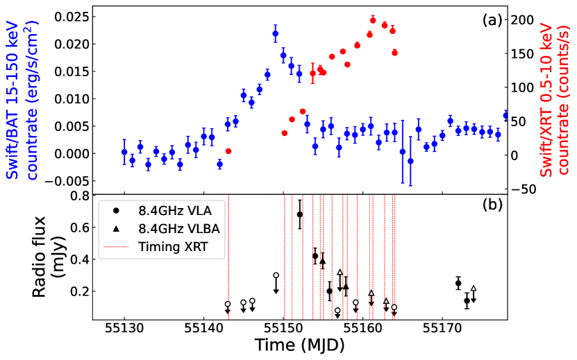
Figure 2: The radio and X-ray light curves of the 2009 outburst of Aql X-1. (a) The observed Swift/XRT and BAT count rates, indicated with red and blue markers respectively. (b) The radio flux densities as first recorded by Miller-Jones et al. (2010). VLA 8.4 GHz and VLBA 8.4 GHz observations are indicated by circles and triangles respectively. Filled markers indicate detections and the corresponding open markers the (3$\sigma$) upper limits. The red dotted lines indicate the timing of the XRT observations.

The aim of this study is to determine the radio/X-ray coupling during this outburst for individual X-ray spectral components. We show the corresponding pairing of observations in Table 1, where observations listed with $X$ and $R$ indicate Swift X-ray and VL(B)A radio observations, respectively. R13 is the only radio observation which was measured within one day of two X-ray observations, but could not be distinctly matched to either: the separation from both XRT observations is approximately equal. Moreover, we find that matching R13 to either X12 or X13 does not significantly impact our results or conclusions in the rest of this work. Therefore, observation R13 is excluded from the analysis. As a second test of the effect of sampling, we decided to combine Swift/XRT spectra to better match the VLA observations in time. We have combined observations X3 and X4 to match R5, X5, X6 and X7 to match R6, X8 and X9 to match R9, and X12, X13, X14 and X15 to match R15. However, this provided no additional insights for this work.

	X-ray	Date	MJD	Duration obs.	ObsID	Time difference	Radio	Date	MJD	Duration obs.	Instrument
	obs.	(2009)	(day)	(ks)		X-R (hour)	obs.	(2009)	(day)	(hour)
	X1	Nov 8	55143.09	2.52	30796036	2.43	R1	Nov 7	55142.99	0.4	VLA
	-	-	-	-	-	-	R2a	Nov 9	55144.97	0.35	VLA
	-	-	-	-	-	-	R3a	Nov 11	55146.09	0.34	VLA
	X2	Nov 15	55150.15	1.00	30796231	25.65	R4	Nov 14	55149.08	0.41	VLA
	X3a	Nov 16	55151.09	1.00	30796232	-	-	-	-	-	-
	X4	Nov 17	55152.44	1.56	30796234	8.82	R5	Nov 17	55152.07	0.39	VLA
	X5	Nov 18	55153.70	1.58	30796235	-7.17	R6	Nov 19	55154	0.82	VLA
	X6a	Nov 19	55154.64	1.52	30796236	-	-	-	-	-	-
	X7	Nov 20	55155.04	1.01	30796237	2.51	R7	Nov 19	55154.94	4.95	VLBA
	X8	Nov 21	55156.11	1.38	30796238	7.25	R8	Nov 20	55155.81	0.81	VLA
	-	-	-	-	-	-	R9a	Nov 21	55156.82	1.07	VLA
	X9	Nov 22	55157.48	0.85	30796239	8.66	R10	Nov 22	55157.12	1.75	VLBA
	X10	Nov 23	55158.05	1.32	30796240	4.62	R11	Nov 22	55157.86	2.26	VLBA
	X11	Nov 24	55159.29	1.33	30796241	4.66	R12	Nov 24	55159.1	0.91	VLA
	X12a	Nov 25	55160.86	1.19	30796242	-	-	-	-	-	-
	-	-	-	-	-	-	R13a	Nov 26	55161.06	3.84	VLBA
	X13a	Nov 26	55161.26	2.28	30796243	-	-	-	-	-	-
	X14	Nov 27	55162.74	1.54	30796244	-4.83	R14	Nov 27	55162.94	4.92	VLBA
	X15a	Nov 28	55163.74	1.27	30796245	-	-	-	-	-	-
	X16	Nov 29	55164.01	1.05	30796246	1.67	R15	Nov 28	55163.94	0.89	VLA

Table 1: Details of the Swift/XRT observations and the corresponding quasi-simultaneous VLA and VLBA 8.4-GHz radio detections and upper limits ($3\sigma$) of Aql X-1. We obtain the archival radio data from Miller-Jones et al. (2010). The MJD for the radio observations are provided for the middle of the observations, and the duration is calculated using the start and stop time for the scans of Aql X-1. The MJD for the X-ray observations are provided for the middle of the observations as well. All X-ray spectra are analysed as elaborated in Section 2. The X-ray and radio observations measured $\lesssim 1$ day apart are matched for the analysis of the radio/X-ray coupling. These data are indicated with red sequential colours from light to dark to indicate the evolution in time in later Figures. ^a These X-ray observations could not be matched to a Radio observation and are therefore excluded from this analysis.

3.2 X-ray spectral model fitting

To calculate the X-ray flux, we fit the Swift/XRT spectra using the composite model as elaborated in Section 2. We aim to determine if adding a black body model component is statistically significant for the XRT spectra, by comparing the models and calculating the F-statistic and its probability. Typically Swift/XRT spectra of NS-LMXBs can be fitted adequately with a power law model, especially at low luminosities (Wijnands et al., 2015). The $\chi^{2}$-statistic for both models and the resulting p-value per observation are shown in Table 2. For the parameter values obtained for the composite model, see Figure 8.

Obs	$\chi^{2}$ dual	$\chi^{2}$ single	p-value	Significance level
	model (d.o.f.)	model (d.o.f.)		p value ($\sigma$)
X1	933.33 (731)	938.59 (732)	4.27E-02	1.72
X2	845.07 (807)	853.86 (808)	3.87E-03	2.66
X3a	514.58 (567)	517.08 (568)	9.75E-02	1.30
X4	932.67 (872)	999.35 (873)	8.65E-15	7.67
X5	935.52 (859)	935.56 (860)	8.48E-01	1.03
X6a	1088.66 (896)	1088.66 (897)	1	-
X7	873.01 (881)	876.6 (882)	5.73E-02	1.58
X8	872.95 (845)	876.27 (846)	7.34E-02	1.45
X9	844.33 (806)	849.91 (807)	2.13E-02	2.03
X10	1386.74 (907)	1386.86 (908)	7.79E-01	0.77
X11	898.53 (856)	898.67 (857)	7.15E-01	0.57
X12a	825.33 (862)	825.33 (863)	1	-
X13a	930.36 (896)	950.14 (897)	1.42E-05	4.19
X14	904.7 (889)	912.83 (890)	4.81E-03	2.59
X15a	924.71 (842)	933.33 (843)	5.20E-03	2.56
X16	845.12 (871)	845.12 (872)	1	-

Table 2: Details of the X-ray spectral fits for the composite (tbabs*(nthcomp+diskbb)) and Comptonised model (tbabs*nthcomp) as elaborated in Section 2. The probability of the F-statistic, or p value, is obtained by comparing the $\chi^{2}$ values and degrees of freedom (d.o.f.) obtained for both models for each observation using ftest in XSPEC. The significance level is obtained using a standard normal distribution ($\mu$=0, $\sigma$=1) for the corresponding probability with a one-tailed test. If the p value exceeds a $2.5\sigma$ confidence level, we consider the contribution of the diskbb component to the model to be significant. See Section 3 for more details.
                                                                                                                                    ^a These X-ray observations could not be matched to a Radio observation and are therefore excluded from this analysis.

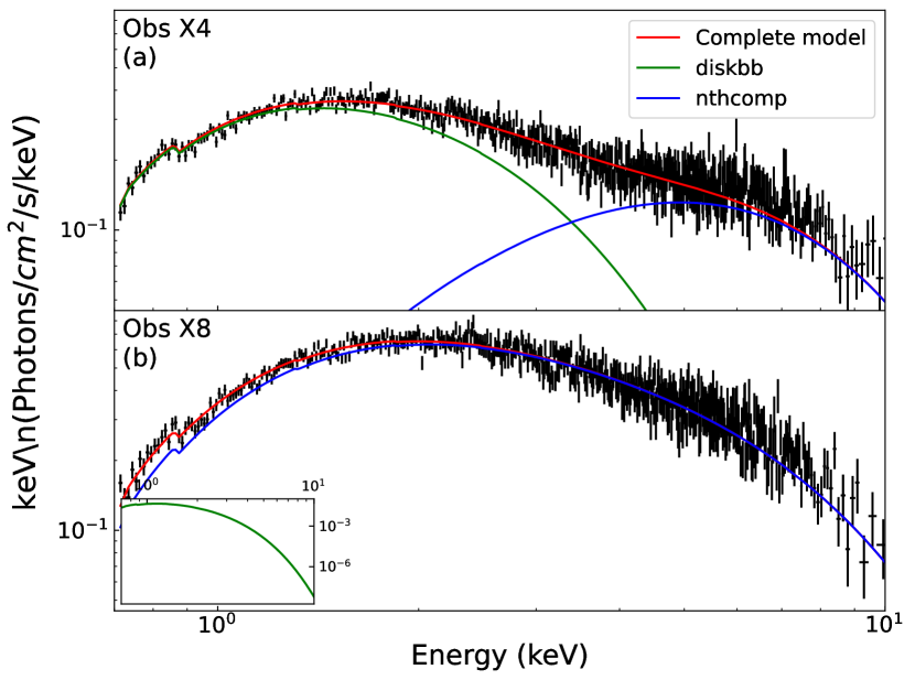
Figure 3: The spectra of observations X4 (Top panel a) and X8 (bottom panel b) plotted with the composite model and the individual model components. The data is shown in black, the complete model in red, and the diskbb and nthcomp model in green and blue, respectively. The data has been visually rebinned (at 5$\sigma$) for clarification. For observation X4 adding the black body component corresponds to a confidence level of 7.67$\sigma$ and is considered significant. For X8 adding the component corresponds to a confidence level of 1.58$\sigma$ and is not considered significant. For observations X8 the diskbb component is so weak compared to the nthcomp component, that we show the diskbb component in the inset for visual purposes, with the scale shown on the right axis.

Initially we consider spectra to have a detectable black body component if the probability of adding the diskbb model component (i.e. using the composite model instead of the Comptonised model) results in a confidence level exceeding $3\sigma$. This requirement is met for observations X4 and X13. However, for observations X2, X14 and X15, this confidence level of adding the thermal component is almost obtained and exceeds $2.5\sigma$, while it is not as significant ($\lesssim 2\sigma$) for the remaining observations. Therefore, for this analysis, we consider X2, X14 and X15 as having a detectable black body component as well. We will further discuss this assumption, and the effect of a broader energy band on these significances, in Section 4.

From our results, it appears that the thermal component intermittently contributes to the model when fitting the spectra. We note a significant contribution for observations X2 and X4 when the hard X-ray flux decays and the soft X-ray flux increases, around MJD 55150 to 55153. We later see a significant contribution for observations X13, X14 and X15, where the soft X-ray flux peaks for the recorded XRT data around MJD 55161 to 55164.

It is important to consider that this could be the result of degeneracies between the thermal and Comptonised model component. In previous studies using RXTE/PCA spectra, the soft state spectra could be fitted using a cool thermal component and a dominant Comptonised component (Gierliński & Done, 2002; Lin et al., 2007). In this case, it is difficult to constrain the temperature and normalisation of the thermal component, and sometimes the thermal component is not required to include in the model. Because of the degeneracies found between the thermal and Comptonised model component for NS-LMXBs, this might not be an accurate model for the spectra in the soft state, also considering other studies finding a strong thermal component in the soft state (e.g. Raichur et al., 2011).

To test whether these degeneracies play a role, we also attempted to first fix parameters to fit a strong thermal component in all observations, and later allowed them to vary, to determine if this changed our results. However, we found that this provided similar results as our earlier fits, which only requires a thermal component for observations X2, X4, X13, X14 and X15. In other words, the lack of detectable thermal component does not arise from initial guesses of parameters and the presence of local minima in the multi-dimensional parameter space.

We can further review the shape of the X-ray spectra. We show an example in Figure 3 comparing the spectra of observations X4 and X8, where X4 has a detectable thermal component and X8 does not. Here, there appears to be a distinction in shape between the two spectra, which could be attributed to the contribution of a strong thermal component in X4. However, since Swift/XRT spectra only cover energies up until 10 keV, this might be biased by the limited energy range over which the fits are performed. We will discuss this in Section 4.

We can also study the evolution in the X-ray colours, to evaluate whether the seemingly intermittent contribution of the thermal component could be related to spectral state transition(s). We define the soft X-ray colour as the ratio between the Swift/XRT countrate in the soft (0.5-2.5 keV) and hard (2.5-10 keV) bands. Secondly, we define the hard X-ray colour as the ratio between the Swift/XRT countrate in WT mode (0.5-10 keV) and the Swift/BAT countrate (15-150 keV). We show the evolution of the individual colours in Figure 4, and the colour-colour diagram is shown in Figure 5. We note that the soft colour initially increases until MJD 55153, after which it decreases again. The soft colour has the highest value for observation X4, where we note the most significant contribution of the black body component. As the soft colour roughly reflects the shape of the spectra measured with XRT between 0.5-10 keV, this result is expected. However, the remaining observations with a significant black body component show lower values for the soft colour. For the hard colour we initially see a decrease, and around MJD 55154 the hard colour levels out. This is reflected in the evolution of the BAT and XRT light curves shown in Figure 2 as well. Based on our results for the BAT and XRT lightcurves, as well as the results for the soft and hard X-ray colour, we conclude that Aql X-1 underwent a transition from a hard to a soft state before MJD 55153.7, and was in the soft state from MJD 55153.7 onward. As mentioned in Section 3.1, the XRT observations stopped after MJD 55164, so we missed the transition back to the hard state as reported by Miller-Jones et al. (2010).

We note that X2 and X4 both show a significant black body component in their spectra and occur during the softening of the soft and hard colour. However, this is not apparent for X13, X14 and X15, which occur after the X-ray colours appear levelled. Furthermore, no significant black body component has been identified for observation X3, which occurs during the spectral softening as well. Therefore, we cannot determine a connection between the transitions of the spectral state and the presence of a significant black body component in the XRT spectra. We return to this point in the Section 4.

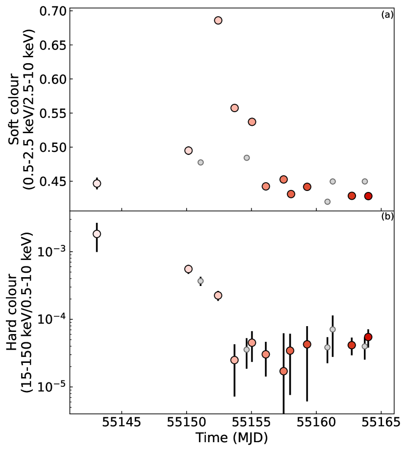
Figure 4: The evolution of Swift X-ray colours throughout the 2009 outburst of Aql X-1. The evolution in time is indicated with red sequential colours from light to dark. The large coloured points indicate the X-ray observations that could be linked to quasi-simultaneous radio observations. Small grey points indicate X-ray observations that could not be linked. (a) The soft X-ray colour, we define this as the ratio between the Swift/XRT count rates in the soft and hard bands. (b) The hard X-ray colour, we define this as the ratio between the Swift/XRT countrate in WT mode and the Swift/BAT orbital countrate.

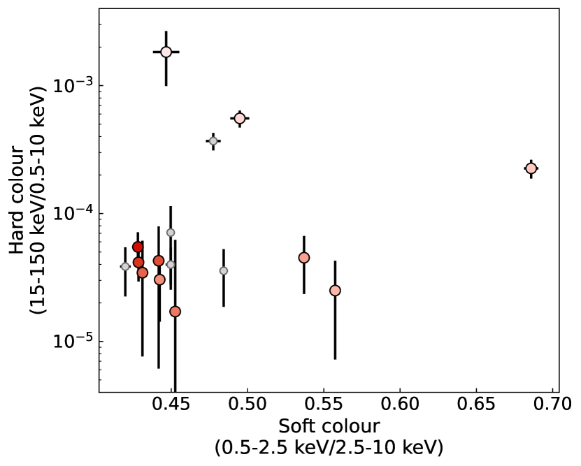
Figure 5: The colour-colour diagram for the 2009 outburst of Aql X-1. The colour coding of the data points and the definition of soft/hard colour used here is the same as in Figure 4.

As elaborated in Section 2, we checked the light curves of the individual X-ray observations for Type-I bursts. We find a Type-I burst in one of the observations, namely in observation X3. However, the thermal component is not detected in this observation with the burst included, and removing the burst does not affect the parameter values for the composite and Comptonised model significantly. For our analysis we have removed the burst in this observation using XSELECT and present the results accordingly.

For the observations where the composite model does not fit significantly better, we determine the $3\sigma$ upper limit of the black body flux as explained in Section 2, by determining the flux where the fit statistic increased (i.e. worsened) by $\Delta\chi^{2}$ = 9. We show the total flux in the composite model, the flux values for both components and the ratio between the thermal flux and the total flux in Figure 6.

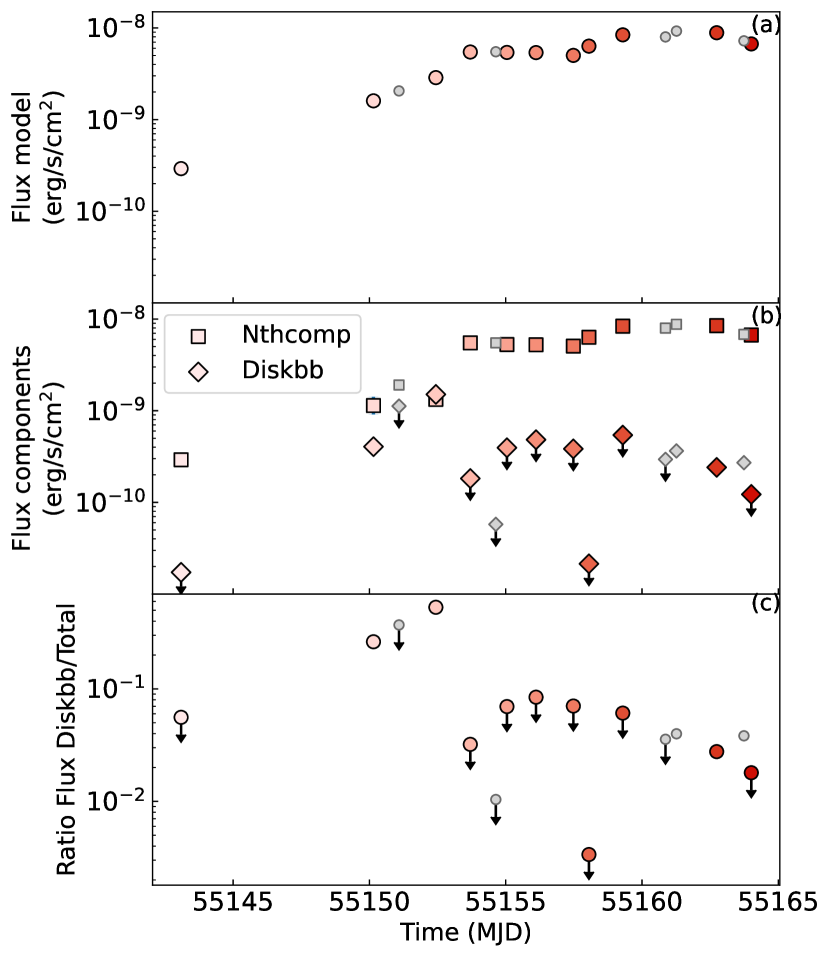
Figure 6: The X-ray flux values obtained for the composite model and the separate model components between 0.7-10 keV. The colour coding of the data points used here is the same as in Figure 4. (a) The X-ray flux calculated for the complete composite model. (b) The X-ray flux for the diskbb and nthcomp model components from 0.7-10 keV. The diskbb and nthcomp component are indicated using diamonds and squares, respectively. (c) The ratio between the X-ray flux for the diskbb component and the total flux.

We note that the total soft X-ray flux initially increases until MJD 55154. The contribution of the diskbb component to the total flux also increases, which coincides with the spectral softening we note in Figure 4. For observations X2 and X4, where the thermal component is detected, the X-ray flux calculated for the diskbb component is around 26.2 to 53.2 percent of the total X-ray flux, respectively. After MJD 55154, the total flux remains somewhat constant until around MJD 55157. The flux then increases again, reaching a peak around MJD 55161, with XRT observations stopping after MJD 55164 due to Sun constraints. Using the RXTE ASM count rate as presented in Miller-Jones et al. (2010), we confirm that the soft X-ray emission (2-10 keV) peaks around this time and decays afterwards. After MJD 55154, the diskbb component contributes considerably less to the total X-ray flux. The majority of XRT observations following MJD 55154 only have upper limits for the diskbb flux. For observations X13 to X15, where the thermal component is detected again, the diskbb component only contributes around 2.8 to 4.0 percent of the total X-ray flux. Therefore, the flux of the nthcomp component contributes substantially to the total flux overall. For most observations the flux for the nthcomp component is at least 91.6 to 99.7 percent of the total soft X-ray flux, considering the upper limit flux values for the diskbb component.

3.3 The radio/X-ray coupling

From our analysis, we find that fitting the composite model only intermittently provides a statistically improved fit to the Comptonised model. Moreover, we find that the flux of the nthcomp component contributes substantially to the total flux overall, and that the flux of the diskbb only contributes around 2.8 to 4.0 percent to the total flux, with the exception of observations X2 and X4. Based on previous work, we find that this could be the result of degeneracies between the thermal and Comptonised component in the composite model, which we will discuss in more detail in Section 4. As we aim to study if the presence of additional thermal emission affects the coupling of the radio/X-ray luminosity, we will explore what the radio/X-ray luminosity plane looks like for this work, keeping in mind that this could be affected by the aforementioned degeneracies. We calculate the X-ray luminosity using the flux from the entire spectrum and from the nthcomp and diskbb components in the composite model separately. We show the resulting radio/X-ray luminosity plane in Figure 7.

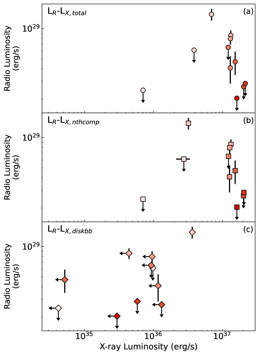
Figure 7: The coupling between the radio and X-ray luminosity, both expressed in erg/s, for the 2009 outburst of Aql X-1. The radio flux densities are obtained at 8.4 GHz and the X-ray flux is calculated between 0.7-10 keV. The evolution in time is indicated with red sequential colours from light to dark. (a) The coupling between the X-ray luminosity calculated for the complete composite model and the radio luminosity. (b) and (c) show this for the X-ray luminosity for the nthcomp and diskbb model components, respectively.

From MJD 55143 to 55151 we see the total X-ray flux increase, including the flux in the diskbb component, as we described in the previous section. This is reflected in Figure 7 as well for the first 2 data points, X1-R1 and X2-R4. During this period, we only measure upper limits for the radio emission. Then the first radio detection coincides with the XRT observation where the nthcomp and diskbb component contribute approximately equally to the total X-ray luminosity, this is data point X4-R5. This is also the observation where the diskbb component is the brightest, which clearly stands out in the Figure at $L_{\mathrm{R}}\approx 1.4\times 10^{29}(d/4.5\text{kpc})^{2}$ erg/s. During these observations, Aql X-1 is transitioning from a hard to a soft state. Once the source is in the soft state around MJD 55154, we note quenching in the radio emission as initially reported by Miller-Jones et al. (2010). Furthermore, we only have upper limits for the diskbb luminosity during this period, with the exception of X14-R14, around $L_{\mathrm{R}}\approx 2.9\times 10^{28}(d/4.5\text{kpc})^{2}$ erg/s.

Overall, we find that with the exception of data point X4-R5, the diskbb luminosity does not contribute substantially to the total X-ray luminosity, nor trends we see in the radio/X-ray coupling before or after the spectral softening. We conclude that separately analysing the component probing the black body emission from the disc, neutron star surface and/or boundary layer, does not reveal a significantly changed radio/X-ray luminosity behaviour for this outburst of Aql X-1.

4 Discussion

4.1 Behaviour of the thermal component

Using archival Swift/XRT data, we have performed a detailed spectral analysis on the X-ray observations obtained from the 2009 outburst of Aql X-1. We have performed this research to study the relative contributions of the thermal black body emission and the Comptonised emission to the radio/X-ray connection derived for this outburst. We find that for these observations, fitting a composite (tbabs*(diskbb+nthcomp)) model intermittently provides a statistically improved fit to a Comptonised (tbabs*nthcomp) model.

As mentioned in Section 3, the Swift/XRT observations cover the rise and apparent peak of soft X-rays during the outburst. We initially observe a spectral softening around MJD 55150 to 55154, where the hard X-ray flux decays and the soft X-ray flux rises, as shown in Figure 2. This softening is reflected in the soft (0.5-2.5 keV) and hard (2.5-10 keV) band of Swift/XRT as shown in Figure 4. For two observations during this transition, namely observations X2 and X4, we find that the thermal black body component diskbb is a significant addition to the model, and the flux calculated for this component contribute arounds 26.2 and 53.2 percent to the total X-ray flux for X2 and X4, respectively. However, this is not the case for observation X3, which is performed during the spectral softening as well. Considering the upper limit found for the diskbb flux, the contribution is less than 37 percent for this observation.

For the majority of the observations following MJD 55154, we can only constrain upper limits for the diskbb component. For the observations where the diskbb component is a significant addition to the model, namely observations X13, X14 and X15, the flux calculated for the thermal component only contributes around 2.8 to 4.0 percent to the total X-ray flux. These observations occur around the peak total flux for the available XRT observations. For the remaining observations the contribution is less then 0.3 to 8.4 percent of the total X-ray flux, considering the upper limit values for the diskbb flux. We show the ratio between the diskbb and total X-ray flux in Figure 6c. Moreover, in Section 3.3 we discuss the contribution of the diskbb luminosity, and conclude that separating the nthcomp and diskbb component does not reveal significantly changed radio/X-ray luminosity behaviour for this outburst.

To explore for the Swift/XRT spectra if the thermal component is present but too faint to detect in the individual observations, we tried to combine the data of observations X5 to X8 and X9 to X12 and fit the composite and Comptonised model to the spectra. The $p$ value of fitting the composite model instead of the Comptonised model is 0.44 for the combined spectrum of observations X5 to X8, corresponding to a significance level of 0.15. The $p$ value of fitting the composite model to the combined spectrum of observations X9 to X12 is 1. This means that during observations X5 to X12, no significant thermal emission is present in the Swift/XRT spectra. The upper limit of the flux in the diskbb component in these spectra is $f_{\rm th}<1.16\times 10^{-10}$ erg/s/cm² for the combined spectrum of observations X5 to X8 and $f_{\rm th}<3.72\times 10^{-11}$ erg/s/cm² for the combined spectrum of observations X9 to X12.

Based on these results, we find that the thermal component is rarely significant in fitting the XRT spectra, with the exception of a few observations. Furthermore, the flux of the thermal black body component contributes less than a few percent of the total X-ray flux in the soft X-ray band for most observations. We conclude that using a Comptonised model (tbabs*nthcomp) is mostly sufficient to fit Swift/XRT spectra for outbursts of Aql X-1. We find no evidence of a significant thermal black body contribution in the Swift/XRT spectra that could cause scatter in the radio/X-ray coupling of Aql X-1, neither in the soft nor in the hard state.

However, we note that we would nominally expect a strong thermal component in the X-ray spectra recorded in the soft state. As spectral degeneracies have been identified between the thermal and Comptonised component in the past (see e.g. Lin et al., 2007), this could be affecting our results with regard to the thermal component.

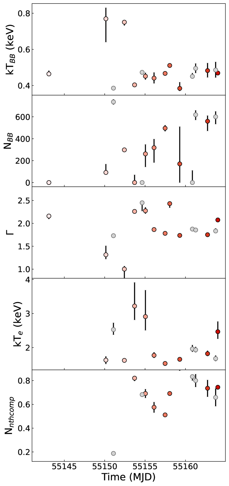
Figure 8: Parameter values of the composite model (tbabs*(diskbb+nthcomp)) for all Swift/XRT spectra. The tbabs model only has the parameter $n_{\mathrm{H}}$, which is fixed to $0.355\times 10^{22}$ cm² for all calculations and fits. Parameters $kT_{\text{bb}}$ (in keV) and $N_{\text{BB}}$ correspond to the diskbb model component. Parameters $\Gamma$, $kT_{\text{e}}$ (in keV) and $N_{\text{nthcomp}}$ (unity at 1 keV for a norm of 1) correspond to the nthcomp model component.

The colour coding of the data points used here is the same as in Figure 4.

One way we can check for degeneracies, is by evaluating the parameter values from our fits. In Figure 8 we show the parameter values for the composite model. For some observations the value for $kT_{\text{e}}$ is pegged at the maximum value for the parameter, around 999 keV. We expect that for these observations no reliable value for the $kT_{\text{e}}$ parameter could be found, possibly because the electron temperature exceeds 10 keV, i.e. outside the XRT passband. Therefore, these data points are not included in the $kT_{\text{e}}$ panel and are set to NaN. For one of the observations, X16, the $N_{\text{BB}}$ parameter is also set to NaN, as adding a diskbb component to the model resulted in a $p$ value of 1. Because the model component is not needed to fit the data properly, this appears to cause some degeneracy in the $N_{\text{BB}}$ parameter for this observation. Furthermore, we also note significant changes in parameter values between consecutive observations. For example, we see the $kT_{\text{bb}}$ and $N_{\text{BB}}$ parameter change significantly from observations X2 to X3 and X3 to X4. As we mentioned in Section 2, this is a known parameter degeneracy, which does not affect the calculations of the flux of the model component. Lastly, we find some degeneracy between the $kT_{\text{bb}}$ and $\Gamma$ parameters for observations X2 to X4 as well.

Based on these findings, we note degeneracies for some fits for the parameters of the diskbb and nthcomp component. However, these might also be indicative of degeneracies between the thermal and Comptonised component, as we note in Section 3.2. As the energy range in the Swift/XRT spectra is limited between 0.7-10 keV, this might affect our ability to constrain the significance of adding a thermal component to the Comptonised model.

To this end, it is important to consider that for our analysis of Swift/XRT, when considering a standard significance level of 3$\sigma$ to add an additional diskbb component to the Comptonised model, only observations X4 and X13 satisfy this requirement. For this analysis, we have considered X2, X14 and X15 to have a significant thermal black body component as well, while the significance level of adding this component ranges between 2.5$\sigma$ and 3$\sigma$. We chose to include these observations as we do not find a comparable significance level for the other observations. In this work we note, for example, that the upper limits we find are not always constraining. We show in Figure 7c that for some observations, the calculated value for the diskbb flux is lower than the upper limits determined for other observations. Consequently, we cannot establish if additional thermal emission is indeed not significant in the latter observations.

To test if adding higher energy coverage might resolve any degeneracies between the thermal and Comptonised component in the composite model, we perform joint fits with quasi-simultaneous RXTE data, which are also presented in (Miller-Jones et al., 2010).

4.2 Joint fits Swift and RXTE spectra

The RXTE/PCA observations are described in Section 2. We matched RXTE/PCA and Swift/XRT observations if they were measured $\la 1$ day from each other. The resulting matched observations are listed in Table 3, and we indicate these with lowercase x1 to x16. To perform the joint fits, we used the same methods as described in Section 2. We added a constant factor to both the RXTE and Swift spectra, and froze this factor for the Swift data at 1, to account for differences in sensitivity and calibration while fitting. Moreover, we also included a gauss model component to the model for the RXTE data, to account for an Fe-K reflection emission line around 6.7 keV (see e.g. Lin et al., 2007). We did not fit a gaussian to the Swift data, as the sensitivity around 6.7 keV is lower than for RXTE, and no gaussian was needed to fit the Swift data properly. The Swift/XRT spectra are fit over the range 0.7-10 keV, and the RXTE PCA spectra over the range 2.6-23 keV. Finally, we calculated the flux over the 0.7-10 keV range, to allow comparison of the joint fits to the results of only fitting the Swift/XRT data.

	X-ray	MJD RXTE	Time difference	MJD Swift
	obs	(day)	Swift-RXTE (hour)	(day)
	x1	55143.07	0.51	55143.09
	x2	55150.28	3.15	55150.15
	x3a	55151.19	2.51	55151.09
	x4	55152.17	6.42	55152.44
	x5	55153.08	14.9	55153.70
	x6a	55154.6	0.89	55154.64
	x7	55155.04	0.11	55155.04
	x8	55156.09	0.53	55156.11
	x9	55157.14	8.18	55157.48
	x10	55157.85	4.86	55158.05
	x11	55158.97	7.78	55159.29
	x12a	55160.15	17.1	55160.86
	x13a	55161.07	4.66	55161.26
	x14	55163.03	6.99	55162.74
	x15a	-	-	55163.74
	x16	55163.94	1.67	55164.01

Table 3: Details of the RXTE observations and the corresponding Swift observations. The MJD are provided for the middle of the X-ray observations. The X-ray observations measured $\la 1$ day apart are matched for the joint fits. These observations are indicated with a lowercase x, in contrast to the uppercase X indicated in Table 1. The data that can be matched with quasi-simultaneous radio data, as described in Table 1, are indicated with purple sequential colours from light to dark to indicate the evolution in time in later Figures.
                                                                                                                                    ^a These X-ray observations could not be matched to a Radio observation and are therefore excluded from this analysis.

We find that fitting the composite model provides a statistically improved fit to the Comptonised model for more observations than we find in our previous results, as shown in Table 4. The thermal component is significant for the joint fits to observations x2-x4, x8-x9 and x11-x16. Only for observations x1, x5-x7, and x10 is the Comptonised model statistically preferred. We note this in particular for observations x5 to x7, as these observations directly follow the transition from the intermediate to the soft state, as discussed in Section 3.2.

Obs	$\chi_{2}$ dual	$\chi_{2}$ single	p-value	Significance level
	model (d.o.f.)	model (d.o.f.)		p value ($\sigma$)
x1	1100.4 (772)	1100.4 (773)	1	-
x2	959.43 (850)	1047.37 (851)	6.06E-18	8.55
x3a	710.59 (609)	835.04 (610)	3.78E-23	9.84
x4	1117.11 (907)	1137.29 (908)	5.61E-05	3.86
x5	1103.4 (896)	1103.4 (897)	1	-
x6a	1171.13 (924)	1171.13 (925)	1	-
x7	907.46 (917)	914.24 (918)	9.00E-03	2.37
x8	951.79 (883)	1071.56 (884)	1.49E-24	10.2
x9	923.12 (849)	992.27 (850)	4.92E-15	7.74
x10	1533.6 (939)	1533.6 (940)	1	-
x11	1013.12 (892)	1140.99 (893)	7.50E-25	10.2
x12a	941.97 (899)	1007.55 (900)	7.46E-15	7.69
x13a	1111.92 (931)	1578.07 (932)	7.95E-73	18.0
x14	1055.74 (921)	1433.79 (922)	3.12E-63	16.7
x15a	-	-	-	-
x16	938.38 (906)	952.18 (907)	2.77E-04	3.45

Table 4: Details of the joint X-ray spectral fits to the Swift/XRT and RXTE/PCA spectra for the composite (tbabs*(nthcomp+diskbb)) and Comptonised model (tbabs*nthcomp). The probability of the F-statistic, or p value, is obtained by comparing the $\chi^{2}$ values and degrees of freedom (d.o.f.) obtained for both models for each observation using ftest in XSPEC. The significance level is obtained using a standard normal distribution ($\mu$=0, $\sigma$=1) for the corresponding probability with a one-tailed test.
                                                                                                                                    ^a These X-ray observations could not be matched to a Radio observation and are therefore excluded from this analysis.

We show the flux for the total model and the individual components in Figure 9, and the parameter values for the composite model in Figure 11. We note that the flux of the diskbb component increases in the soft state, but that at the start of the soft state (x5-x7) we only have upper limits for the thermal flux. We note that these fits can still be affected by spectral degeneracies between the thermal and Comptonised component as discussed previously. However, we also note that the upper limits found for the diskbb flux are more constraining than those for the Swift/XRT spectra. We also find that the ratio between the diskbb flux and the total flux is around $26\%$ at x2, after which the contribution decreases, and gradually increases again in the soft state, contributing around $26.1\%$ at the peak of the soft X-ray flux around x14.

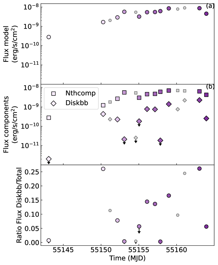
Figure 9: The X-ray flux values obtained for the joint fits to the Swift/XRT and RXTE/PCA spectra for composite model and the separate model components between 0.7-10 keV. The evolution in time is indicated with purple sequential colours from light to dark. The large coloured points indicate the X-ray observations that could be linked to quasi-simultaneous radio observations. Small grey points indicate X-ray observations that could not be linked. (a) The X-ray flux calculated for the complete composite model from 0.7-10 keV. (b) The X-ray flux for the diskbb and nthcomp model components. The diskbb and nthcomp component are indicated using diamonds and squares, respectively. (c) The ratio between the X-ray flux for the diskbb component and the total flux.

Putting the results of the joint fits in the context of the radio/X-ray luminosity plane in Figure 10, we see that the luminosity for the diskbb component increases as the radio luminosity quenches. However, we still find that the radio/X-ray coupling is not significantly changed when we separate emission from a thermal component.

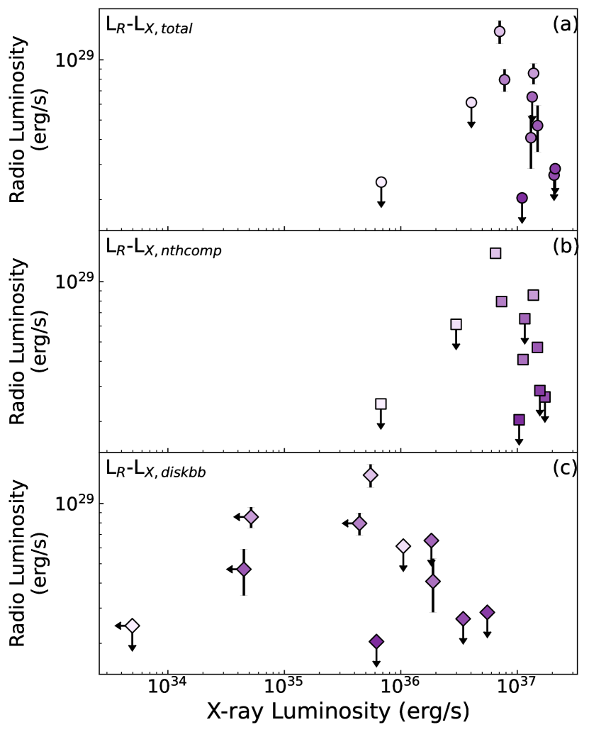
Figure 10: The coupling between the radio and X-ray luminosity, where the X-ray luminosity is obtained from the joint fits to the Swift/XRT and RXTE/PCA spectra. The radio flux densities are obtained at 8.4 GHz and the X-ray flux is calculated between 0.7-10 keV. The evolution in time is indicated with purple sequential colours from light to dark. (a) The coupling between the X-ray luminosity calculated for the complete composite model and the radio luminosity. (b) and (c) show this for the X-ray luminosity for the nthcomp and diskbb model components, respectively.

Overall, performing joint fits with Swift/XRT and RXTE/PCA appears to have resolved some of the spectral degeneracies that might have affected the fits to the Swift/XRT spectra. However, our conclusions regarding the radio/X-ray coupling remain unchanged. Moreover, we still find that the thermal component is not always a significant addition to modelling the X-ray spectra. Therefore, this analysis should be followed up with more sensitive, broad-band X-ray observations and densely-sampled near-simultaneous radio observations in the future (see Section 4.4).

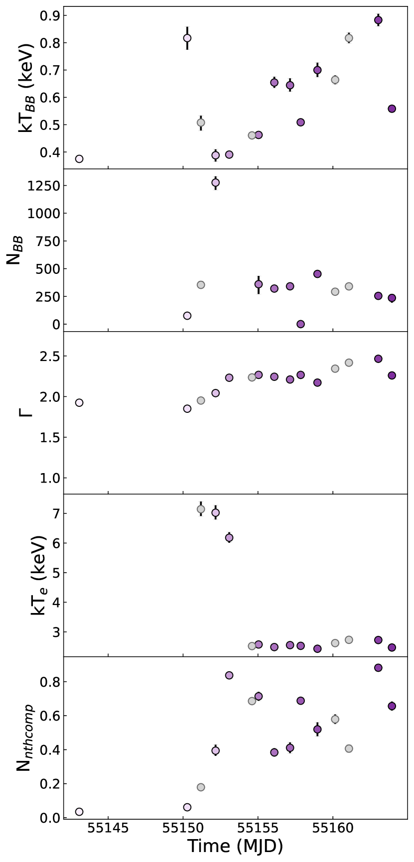
Figure 11: Parameter values obtained for the joint fits to the Swift/XRT and RXTE/PCA spectra for composite model. The tbabs model only has the parameter $n_{\mathrm{H}}$, which is fixed to $0.355\times 10^{22}$ cm² for all calculations and fits. Parameters $kT_{\text{bb}}$ (in keV) and $N_{\text{BB}}$ correspond to the diskbb model component. Parameters $\Gamma$, $kT_{\text{e}}$ (in keV) and $N_{\text{nthcomp}}$ (unity at 1 keV for a norm of 1) correspond to the nthcomp model component. The colour coding of the data points used here is the same as in Figure 9.

4.3 Interpretation jet/accretion behaviour

Since our results can be affected by degeneracies between the thermal and Comptonised component, there are issues in constraining the contribution of the thermal component in our X-ray spectra. Therefore, it is difficult to interpret the results to study the physical processes. However, we can consider the implications of our results to the radio/X-ray coupling, to discuss what this would mean for the jet/accretion behaviour if these degeneracies were not present.

In this case, our results seem to partially agree with the behaviour of the accretion flow and jets in some BH-LMXB sources. For transient outbursts of BH-LMXBs, one observes compact jets during the hard state, and the jets persist until the X-ray spectrum softens (Fender et al., 2004). Once the source transitions to the soft state, one notes quenching of the jet (see e.g. Gallo et al., 2003; Russell et al., 2011; Coriat et al., 2011). For some sources, radio emission has been detected with a negative spectral slope during the bright hard to soft state transition near the peak of the outburst. This is interpreted as being associated with the scenario where the core jet is suppressed once the accretion disc propagates inwards toward the innermost stable circular orbit (ISCO). In this scenario the optically thin radio emission is associated with jet ejecta probing the re-brightening at shocks from the jet propagating away from the BH-LMXB (Fender et al., 2004, 2009). When the source transitions back to the hard state, one observes compact jets again (see e.g. Kalemci et al., 2005, 2013).

For Aql X-1, some of these features have been observed as well. Díaz Trigo et al. (2018) reports radio to millimetre emission with a negative slope during the 2016 outburst of Aql X-1 after the transition to the soft state. Furthermore, Tudose et al. (2009) has studied the outbursts in 2002, 2004 and 2005 using multiwavelength data, and found that the radio emission quenched above a critical X-ray luminosity of around 10 percent of the Eddington luminosity. Tudose et al. (2009) suggest this could be similar behaviour as seen for BH-LMXBs like we mentioned previously.

For the 2009 outburst, only one constraint could be placed on the spectral slope of the radio emission. Using the 8.4 GHz VLBA observation (labelled R7 in this work) and the 5 GHz EVN observation between MJD 55154 and 55155, Miller-Jones et al. (2010) find a slightly inverted slope of $\alpha=0.40\pm 0.31$, which is detected after the transition to the soft state.

We are particularly interested in the radio observations during the bright transition from the hard to the soft state, to see if Aql X-1 could show transient jet ejecta like those observed for BH-LMXBs. Unfortunately, we have no constraints on the spectral slope of the radio emission in this period. However, we do find that the first and brightest detection of radio emission R5 coincides with X4/x4. Based on our spectral analysis of the Swift/XRT spectra, we find that X4 has the brightest thermal component. From our joint fits with the RXTE data, we find a significantly lower diskbb flux for x4. However, we also see that between X1 and X4 the soft colour for Swift/XRT increases, and peaks for observation X4. This could be indicative of the disc moving toward the ISCO during the transition from the hard and the soft state, i.e. between X1 and X4, causing the material in the disc to heat up and the thermal component to become brighter. This could potentially result in more flux in the soft X-ray band (0.5-2.5 keV) when compared to the hard X-ray band (2.5-10 keV).

Following radio observation R5, we note quenching in the radio emission, as initially reported by Miller-Jones et al. (2010). This happens at a total X-ray luminosity of around $L_{\mathrm{X}}=1.3\times 10^{37}(d/4.5\text{kpc})^{2}$ erg/s. This also fits the scenario seen for BH-LMXBs, where the radio emission quenches once the source transitions to the soft state. Once the source is in the soft state and the jet quenches, we mainly find upper limits for the luminosity of the diskbb component, with the exception of observations X13 to X15, when we only look at the results for the Swift/XRT spectra. For the joint fits with Swift/XRT and RXTE/PCA, we find that $kT_{\text{bb}}$ and the contribution of the thermal component increases in the soft state from x7 on. In both cases, the detected thermal emission could probe the disc heating up again, as it coincides with the apparent peak of the soft X-ray emission.

We also consider if the thermal emission in observations X2 to X4 probes another emission process than the thermal emission in later observations, as we only find a significant thermal component in X13 to X15 for the Swift/XRT spectra. For example, Wijnands et al. (2015) found that for the accretion flow of NS-LMXBs at low luminosities, the thermal emission from the neutron star surface can dominate the spectrum. To explore this scenario, we may study the parameter values obtained for the composite model, especially the $kT_{\text{bb}}$ parameter. However, due to parameter degeneracies as discussed in Section 4.1, we were unable to determine this for the Swift/XRT spectra. For the joint Swift/XRT and RXTE/PCA fits, we find that $kT_{\text{bb}}$ is around 0.77 keV at x2, then the temperature appears to decrease, and gradually increases again in the soft state. A similar pattern in seen for the contribution of the diskbb flux to the total flux. However, this could again be the result of the parameter degeneracy between $kT_{\text{bb}}$ and $N_{\text{BB}}$. For x4, we note a relatively low value for $kT_{\text{bb}}$, and a peak value for the $N_{\text{BB}}$ parameter. Therefore, we are unable to link these results for the thermal emission to a specific emission process.

Based on our results, we cannot confirm that the thermal emission detected in the Swift/XRT spectra nor the joint Swift/XRT and RXTE/PCA fits probe the accretion disc in particular. The scenario proposed for the jet/accretion coupling for some BH-LMXBs appears to match our results, where the disc moves toward the ISCO and bright transient jet ejecta are observed during the transition from the hard to the soft state, and later the radio emission from the jet quenches in the soft state. However, we need more information to unambiguously determine the jet/accretion behaviour for Aql X-1, and to be able to compare the behaviour of BH-LMXB and NS-LMXB sources.

4.4 Future research

More sensitive observations could allow us to identify separate spectral components probing the emission of the NS surface, boundary layer and accretion disc, while only one thermal component could be identified in this work. One telescope that we propose for follow-up research is the Neutron star Interior Composition Explorer (NICER, Gendreau et al., 2016). Simple spectral simulations, detailed in Appendix A, show how short NICER monitoring observations are able to establish the presence of a thermal component down to significantly lower thermal luminosities. An extension of this work using NICER and radio monitoring therefore allows for more detailed follow-up studies. However, we also stress that these simulations operate under the assumption that the input model is correct, i.e. that only statistical uncertainties play a role. That assumption implies that the complications with this analysis, such as model degeneracies in the absence of hard X-ray coverage, will remain for NICER as well.

These issues of parameter degeneracy and broad-band energy converage may be alleviated more effectively through future missions. For instance, the proposed Strobe-X mission (Ray et al., 2019) is planned to combine a soft (0.2-12 keV) instrument, the X-ray Concentrator Array, as well as a harder (2-30 keV) instrument, the Large Area Detector. Alternatively, the proposed HEX-P mission is planned to combine two detectors, the Low Energy Telescope and the High Energy Telescope, to provide simultaneous spectral coverage between 0.1 and 150 keV (Madsen et al., 2019). The broad-energy coverage of both observatories may remove the issues found in our work with model degeneracies, while syngergies with next generation radio observatories could allow for follow up studies at unprecedented sensitivity. An essential requirement, for this purpose, however is sufficient flexibility to allow for high cadence monitoring of an LMXB outburst, similar to RXTE, Swift, and NICER.

Data availability

The data underlying this article will be available in Zenodo at DOI: 10.5281/zenodo.6477045 upon publication. These astrophysical data sets were derived from archival radio data reported by Miller-Jones et al. (2010) and X-ray data from sources in the public domain: https://heasarc.gsfc.nasa.gov/cgi-bin/W3Browse/swift.pl.

Appendix A NICER simulations

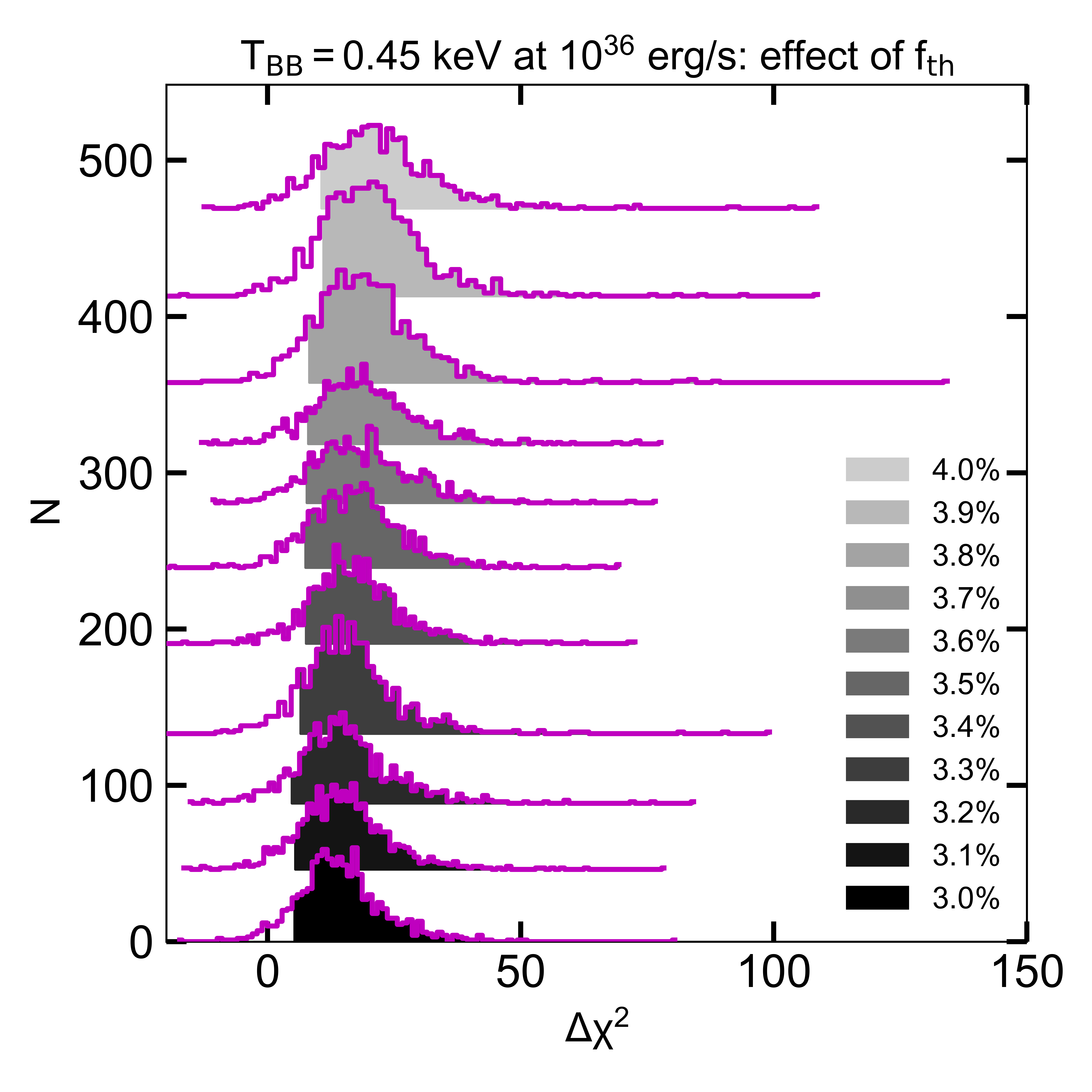
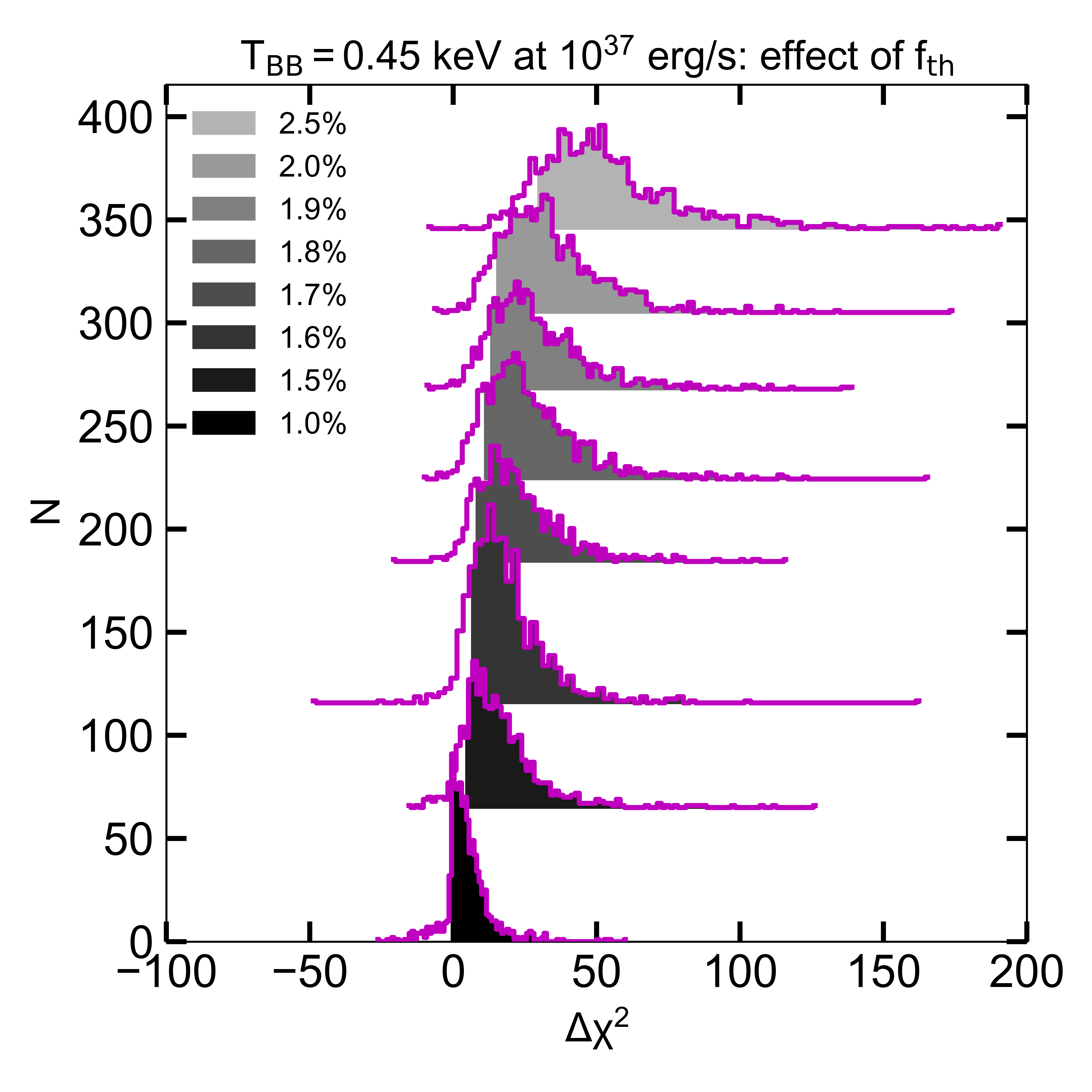
Figure A1: Histograms of the fit improvement $\Delta\chi^{2}$ when comparing fits of a synthetic NICER spectrum, simulated with the indicated $L_{\mathrm{X}}$ and $f_{\rm th}$, with both an absorbed nthcomp and the composite model. The histograms are vertically offset for clarity. The shaded region includes the highest $90$% of $\Delta\chi^{2}$ values.

In order to assess whether the Neutron star Interior Composition Explorer (NICER, Gendreau et al., 2016) could be used to established the presence of thermal emission to lower X-ray fluxes, we performed a suite of X-ray spectral simulations. Using the fakeit task in xspec, we simulated spectra following the tbabs*(diskbb+nthcomp) model used in this work. Each simulated spectrum was then fitted with both the full model, assuming the same constraints as in the main paper (i.e. fixed $n_{\mathrm{H}}=0.355\times 10^{22}$ cm^-2, linked disc and seed photon temperatures), and the simpler tbabs*nthcomp model. Linking the temperatures means that the composite model has one more free parameter, implying that a fit improvement of $\Delta\chi^{2}=9$ is significant at the $3\sigma$ level. With our simulations, we set out to find the minimum fractional flux in the thermal component, that would leave the thermal component $3\sigma$ detectable in at least $90\%$ of the simulated spectra.

As input for the simulated spectra, we assumed either $L_{\mathrm{X}}=10^{37}$ erg/s or $L_{\mathrm{X}}=10^{36}$ erg/s. We set $\Gamma=2$, $kT_{e}=1.8$ keV, and $kT_{\rm BB}=0.45$ keV, as typical values found in our analysis of Aql X-1. We also assumed $d=4.5$ kpc to convert luminosities to fluxes. The normalisations of the diskbb and nthcomp components were determined such that the thermal, unabsorbed flux equaled $f_{\rm th}\times L_{X}/4\pi d^{2}$, compared to a non-thermal unabsorbed flux of $(1-f_{\rm th})\times L_{\mathrm{X}}/4\pi d^{2}$. In the simulations, we used the NICER response and background files for an observation of Aql X-1 with an exposure of $\sim 1$ ks (ObsID 2050340127): after accessing the observation files, we ran nicerl2 to re-reduce the data and subsequently applied standard routines using nicerarf, nicerrmf, and the python package nicergof.bkg to generate the arf and rmf files, and background spectrum. Each spectrum was similated for an exposure time of $1$ ks; for each setup of input parameters ($L_{\mathrm{X}}$, $f_{\rm th}$) we performed 1000 runs, each run saving the fit improvement $\Delta\chi^{2}$.

In Figure A1, we show the histograms of the resulting $\Delta\chi^{2}$ values for each combination of $L_{\mathrm{X}}$ ($10^{36}$ erg/s left; $10^{37}$ erg/s right) and $f_{\rm th}$. The histograms are vertically offset for clarity. The shaded regions, corresponding to the $f_{\rm th}$ indicated in the legend, indicate $90$% of the $1000$ runs. As we define $\Delta\chi^{2}\geq 9$ as a significant detection of the thermal component, we search for the minimum $f_{\rm th}$ where the shaded region lies fully at $\Delta\chi^{2}\geq 9$. We find that at $L_{\mathrm{X}}=10^{36}$ erg/s, $f_{\rm th}\geq 3.9$% is detectable in $\geq 90$% of simulated spectra. For $L_{\mathrm{X}}=10^{37}$ erg/s, this limit drops to $f_{\rm th}\geq 1.8\%$. These limits are significantly lower than most of the Swift limits reported in the main paper (c.f. Figure 2, bottom panel; $L_{\mathrm{X}}=10^{37}$ erg/s corresponds to $\sim 4\times 10^{-9}$ erg/s/cm²), especially at the higher of the two luminosities.

These results are simplified, in terms of the other spectral parameters: the exact values of the other broadband parameters will influence the actual significance of a thermal component, especially close to the $3\sigma$ threshold. However, these simulations indicate the promise of using NICER monitoring of an extension of the main paper to other sources and outbursts.

References

- Arnaud (1996) Arnaud K. A., 1996, in Jacoby G. H., Barnes J., eds, Astronomical Society of the Pacific Conference Series Vol. 101, Astronomical Data Analysis Software and Systems V. p. 17
- Babkovskaia et al. (2008) Babkovskaia N., Brandenburg A., Poutanen J., 2008, MNRAS, 386, 1038
- Bright et al. (2020) Bright J. S., et al., 2020, Nature Astronomy, 4, 697
- Campana et al. (2013) Campana S., Coti Zelati F., D’Avanzo P., 2013, MNRAS, 432, 1695
- Cannizzo (1993) Cannizzo J. K., 1993, ApJ, 419, 318
- Carotenuto et al. (2021a) Carotenuto F., et al., 2021a, MNRAS, 504, 444
- Carotenuto et al. (2021b) Carotenuto F., et al., 2021b, MNRAS, 505, L58
- Chevalier & Ilovaisky (1991) Chevalier C., Ilovaisky S. A., 1991, A&A, 251, L11
- Chevalier et al. (1999) Chevalier C., Ilovaisky S. A., Leisy P., Patat F., 1999, A&A, 347, L51
- Corbel et al. (2000) Corbel S., Fender R. P., Tzioumis A. K., Nowak M., McIntyre V., Durouchoux P., Sood R., 2000, A&A, 359, 251
- Corbel et al. (2002) Corbel S., Fender R. P., Tzioumis A. K., Tomsick J. A., Orosz J. A., Miller J. M., Wijnands R., Kaaret P., 2002, Science, 298, 196
- Corbel et al. (2003) Corbel S., Nowak M. A., Fender R. P., Tzioumis A. K., Markoff S., 2003, A&A, 400, 1007
- Coriat et al. (2011) Coriat M., et al., 2011, MNRAS, 414, 677
- Díaz Trigo et al. (2018) Díaz Trigo M., et al., 2018, A&A, 616, A23
- Done et al. (2007) Done C., Gierliński M., Kubota A., 2007, A&ARv, 15, 1
- Evans et al. (2007) Evans P. A., et al., 2007, A&A, 469, 379
- Evans et al. (2009) Evans P. A., et al., 2009, MNRAS, 397, 1177
- Fender & Muñoz-Darias (2016) Fender R., Muñoz-Darias T., 2016, The Balance of Power: Accretion and Feedback in Stellar Mass Black Holes. p. 65, doi:10.1007/978-3-319-19416-5_3
- Fender et al. (1999) Fender R., et al., 1999, ApJ, 519, L165
- Fender et al. (2004) Fender R. P., Belloni T. M., Gallo E., 2004, MNRAS, 355, 1105
- Fender et al. (2009) Fender R. P., Homan J., Belloni T. M., 2009, MNRAS, 396, 1370
- Friedman et al. (1967) Friedman H., Byram E. T., Chubb T. A., 1967, Science, 156, 374
- Gallo et al. (2003) Gallo E., Fender R. P., Pooley G. G., 2003, MNRAS, 344, 60
- Gallo et al. (2018) Gallo E., Degenaar N., van den Eijnden J., 2018, MNRAS, 478, L132
- Galloway et al. (2008) Galloway D. K., Muno M. P., Hartman J. M., Psaltis D., Chakrabarty D., 2008, ApJS, 179, 360
- Gehrels et al. (2004) Gehrels N., et al., 2004, ApJ, 611, 1005
- Gendreau et al. (2016) Gendreau K. C., et al., 2016, in den Herder J.-W. A., Takahashi T., Bautz M., eds, Society of Photo-Optical Instrumentation Engineers (SPIE) Conference Series Vol. 9905, Space Telescopes and Instrumentation 2016: Ultraviolet to Gamma Ray. p. 99051H, doi:10.1117/12.2231304
- Gierliński & Done (2002) Gierliński M., Done C., 2002, MNRAS, 337, 1373
- Gilfanov (2010) Gilfanov M., 2010, X-Ray Emission from Black-Hole Binaries. p. 17, doi:10.1007/978-3-540-76937-8_2
- Güngör et al. (2017) Güngör C., Ekşi K. Y., Göğüş E., Güver T., 2017, ApJ, 848, 13
- Gusinskaia et al. (2017) Gusinskaia N. V., et al., 2017, MNRAS, 470, 1871
- Gusinskaia et al. (2020) Gusinskaia N. V., et al., 2020, MNRAS, 492, 2858
- Hameury et al. (2000) Hameury J.-M., Lasota J.-P., Warner B., 2000, A&A, 353, 244
- Hannikainen et al. (1998) Hannikainen D. C., Hunstead R. W., Campbell-Wilson D., Sood R. K., 1998, A&A, 337, 460
- Harmon et al. (1995) Harmon B. A., et al., 1995, Nature, 374, 703
- Hjellming & Wade (1971) Hjellming R. M., Wade C. M., 1971, ApJ, 164, L1
- Homan et al. (2010) Homan J., et al., 2010, ApJ, 719, 201
- Jahoda et al. (1996) Jahoda K., Swank J. H., Giles A. B., Stark M. J., Strohmayer T., Zhang W., Morgan E. H., 1996, in Siegmund O. H., Gummin M. A., eds, Society of Photo-Optical Instrumentation Engineers (SPIE) Conference Series Vol. 2808, EUV, X-Ray, and Gamma-Ray Instrumentation for Astronomy VII. pp 59–70, doi:10.1117/12.256034
- Kalemci et al. (2005) Kalemci E., Tomsick J. A., Buxton M. M., Rothschild R. E., Pottschmidt K., Corbel S., Brocksopp C., Kaaret P., 2005, ApJ, 622, 508
- Kalemci et al. (2013) Kalemci E., Dinçer T., Tomsick J. A., Buxton M. M., Bailyn C. D., Chun Y. Y., 2013, ApJ, 779, 95
- Koyama et al. (1981) Koyama K., et al., 1981, ApJ, 247, L27
- Kreykenbohm et al. (2004) Kreykenbohm I., Wilms J., Coburn W., Kuster M., Rothschild R. E., Heindl W. A., Kretschmar P., Staubert R., 2004, A&A, 427, 975
- Krimm et al. (2013) Krimm H. A., et al., 2013, ApJS, 209, 14
- Kunte et al. (1973) Kunte P. K., Durgaprasad N., Gokhale G. S., Iyengar V. S., Manchanda R. K., Sreekantan B. V., 1973, Nature Physical Science, 245, 37
- Lasota (2001) Lasota J.-P., 2001, New Astron. Rev., 45, 449
- Lin et al. (2007) Lin D., Remillard R. A., Homan J., 2007, ApJ, 667, 1073
- Maccarone & Coppi (2003) Maccarone T. J., Coppi P. S., 2003, MNRAS, 338, 189
- Madsen et al. (2019) Madsen K., et al., 2019, in Bulletin of the American Astronomical Society. p. 166
- Markwardt et al. (2000) Markwardt C. B., Swank J. H., Marshall F. E., in’t Zand J. J. M., 2000, in Strohmayer T. E., ed., Rossi2000: Astrophysics with the Rossi X-ray Timing Explorer. p. 7
- Migliari & Fender (2006) Migliari S., Fender R. P., 2006, MNRAS, 366, 79
- Migliari et al. (2003) Migliari S., Fender R. P., Rupen M., Jonker P. G., Klein-Wolt M., Hjellming R. M., van der Klis M., 2003, MNRAS, 342, L67
- Migliari et al. (2004) Migliari S., Fender R. P., Rupen M., Wachter S., Jonker P. G., Homan J., van der Klis M., 2004, MNRAS, 351, 186
- Migliari et al. (2011) Migliari S., Tudose V., Miller-Jones J. C. A., Kuulkers E., Nakajima M., Yamaoka K., 2011, The Astronomer’s Telegram, 3198, 1
- Miller-Jones et al. (2010) Miller-Jones J. C. A., et al., 2010, ApJ, 716, L109
- Paczynski (1971) Paczynski B., 1971, Annual Review of Astronomy and Astrophysics, 9, 183
- Raichur et al. (2011) Raichur H., Misra R., Dewangan G., 2011, MNRAS, 416, 637
- Ray et al. (2019) Ray P. S., et al., 2019, ] 10.48550/ARXIV.1903.03035
- Reig et al. (2000) Reig P., Méndez M., van der Klis M., Ford E. C., 2000, ApJ, 530, 916
- Russell et al. (2011) Russell D. M., Miller-Jones J. C. A., Maccarone T. J., Yang Y. J., Fender R. P., Lewis F., 2011, ApJ, 739, L19
- Russell et al. (2019) Russell T. D., et al., 2019, ApJ, 883, 198
- Russell et al. (2021) Russell T. D., et al., 2021, MNRAS, 508, L6
- Sakurai et al. (2012) Sakurai S., Yamada S., Torii S., Noda H., Nakazawa K., Makishima K., Takahashi H., 2012, PASJ, 64, 72
- Shakura & Sunyaev (1973) Shakura N. I., Sunyaev R. A., 1973, A&A, 500, 33
- Sibgatullin & Sunyaev (1998) Sibgatullin N. R., Sunyaev R. A., 1998, Astronomy Letters, 24, 774
- Thorstensen et al. (1978) Thorstensen J., Charles P., Bowyer S., 1978, ApJ, 220, L131
- Tudose et al. (2009) Tudose V., Fender R. P., Linares M., Maitra D., van der Klis M., 2009, MNRAS, 400, 2111
- Van den Eijnden et al. (2021) Van den Eijnden J., et al., 2021, MNRAS, 507, 3899
- Verner et al. (1996) Verner D. A., Ferland G. J., Korista K. T., Yakovlev D. G., 1996, ApJ, 465, 487
- Wijnands et al. (2015) Wijnands R., Degenaar N., Armas Padilla M., Altamirano D., Cavecchi Y., Linares M., Bahramian A., Heinke C. O., 2015, MNRAS, 454, 1371
- Wilms et al. (2000) Wilms J., Allen A., McCray R., 2000, ApJ, 542, 914
- Yu et al. (2003) Yu W., Klein-Wolt M., Fender R., van der Klis M., 2003, ApJ, 589, L33