Chirality distributions inside baryons in ${\rm QCD_{2}}$

Abstract

The connection between the spin distribution and the topological structure of the baryon is an open and important problem. Here we address it using QCD in $(1+1)$ spacetime dimensions, which is exactly solvable at large number of colors $N$. It is found that the distribution of chirality inside a baryon is drastically different from a chirality distribution inside states with zero baryon number, “mesons”. This difference is shown to arise from the topological structure of the baryon – at large $N$, all of the baryon’s chirality is concentrated near $x=0$, whereas in a meson state it vanishes in the small $x$ limit. Our results illustrate how the constituent features of the baryon reemerge and are tied to the topological features of the bosonized solitonic solution. Possible implications for QCD in $(3+1)$ dimensions and for deep inelastic scattering experiments are discussed.

I Introduction

Quantum chromodynamics (QCD) is the established fundamental theory of strong interactions. Nevertheless, the ways in which the properties of hadrons and their interactions emerge from this microscopic theory remain poorly understood. Two of the most interesting open problems are the confinement of quarks and the distribution of the baryon’s spin among its constituents. The latter is usually addressed within the parton model that does not fully take into account the nonperturbative structure of the baryon (which only enters through the initial conditions in the Dokshitzer–Gribov–Lipatov–Altarelli–Parisi (DGLAP) parton evolution equations). This lack of connection between the nonperturbative and perturbative sides of the problem may in fact be at the origin of the difficulties in theoretical understanding of the spin distribution inside the proton, or the “proton spin puzzle” (see [1, 2, 3, 4, 5, 6] for reviews).

In this paper, we address the connection between the nonperturbative structure of the baryon and the spin (or rather, chirality) distribution inside of it using QCD in $(1+1)$ dimensions, QCD₂. This model is exactly solvable in the limit of large number of colors $N$ and is known to share many properties with QCD₄, including confinement, mass gap generation, and spontaneous breaking of chiral symmetry [7, 8, 9, 10].

While the notion of spin is absent in one spatial dimension, what is often meant by the “spin” structure of the proton in high-energy interactions, even in four spacetime dimensions, is really its chirality content, which is perfectly well-defined in two spacetime dimensions. Furthermore, at high energy, dimensional reduction leads to the separation of transverse and longitudinal degrees of freedom, so that ($1+1$)-dimensional dynamics may be more relevant for understanding QCD₄ than naively expected. Crucially, large $N$ QCD₂ is an exactly solvable model, valid at all energy scales, which will allow us to address the effect of hadron topological structure on the chirality distribution.

Indeed, the internal topology of the baryon may affect the chirality distribution inside of it. It has long been known [11, 12] that baryons can be described as topological solitons. The importance of this topological structure for the spin distribution has already been addressed in the context of the Skyrme model [13]. It has been found that the chirality of valence quarks does not contribute to the spin of the baryon, and all of it arises from the topology of the Skyrmion solution. However in $(3+1)$ dimensions, the Skyrme model represents an effective low-energy description of QCD - therefore its validity at short distances, and thus the relevance for the interpretation of the data from deep inelastic scattering (DIS) can be questioned. In contrast, in QCD₂ the topological description applies at all energy scales, and will allow us to investigate the effect of baryon topology on its chirality distribution from first principles.

In the ’t Hooft limit ($N\to\infty$, $g^{2}N$ fixed), QCD₂ reduces to an interacting sine-Gordon model [14, 15, 16]. In this bosonic description, the baryon emerges as a topological soliton solution – a kink. In this work, we apply ideas from [17] to describe the quantum soliton state in terms of its constituents. This decomposition is analogous to the parton model in QCD₄, but fully takes account of the topological structure of the soliton. We then use this decomposition to evaluate the chirality distribution inside the soliton.

This paper is organized as follows. We motivate our calculation from the proton spin problem point of view in section II.1. We then review some properties of QCD₂ and of the sine-Gordon model in sections II.2 and II.3. Section III contains the original results of this work. In section III.1 we extend the results of [17] on quantum solitons to the sine-Gordon model. We then use these results in section III.2 to define and compute the matrix elements of axial current, representing a $(1+1)$ analog of the polarized structure function $g_{1}(x_{B})$ ($x_{B}$ is the Bjorken $x$). We conclude in section IV with a discussion of these results and their possible implications for the $(3+1)$-dimensional QCD and the spin structure of the baryons. For the sake of self-completeness, in appendix  A there is a pedagogical review of deep inelastic scattering and of the proton “spin crisis”.

II The proton spin, topology, and the Sine-Gordon model

II.1 Motivation

Before moving on to $(1+1)$ dimensions, let us briefly recall the role chirality distributions play in spin distributions. We refer the interested reader to Appendix A and references therein for more detailed information about $3+1$ spin physics.

The matrix elements describing the interaction of hadrons with the electromagnetic field are parametrized in terms of structure functions which need to be measured experimentally or evaluated in lattice simulations. Of its spin dependent parts, the proton polarized structure function $g_{1}(x_{B})$ is of particular interest [see eq. (A) for its definition and eq.(50) for the kinematic definition of the Bjorken $x_{B}$]. It is experimentally measured in polarized deep inelastic scattering. Moreover, perturbative QCD relates its first Mellin moment to the axial charges of the nucleon:

$$\int_{0}^{1}\mathrm{d}x_{B}g_{1}(x_{B})=\frac{1}{12}a^{3}+\frac{1}{36}a^{8}+\frac{1}{9}a^{0}\ ,$$ (1)

where the axial charges $a^{3},a^{8},a^{0}$ are related to the matrix elements of the corresponding QCD currents over the proton state:

$$2Ms^{\mu}a^{k}\propto\langle\mathrm{p},s|j_{5}^{\mu(k)}|\mathrm{p},s\rangle.$$ (2)

With $a^{3}$ and $a^{8}$ inferred from independent experiments, polarized DIS provides a measurement of the axial charge $a^{0}$ and polarized quark distributions. In other words, it probes the chirality distribution inside a hadron. It is yet unknown how the different internal structures of baryons and mesons affect their chirality distributions. To make progress toward answering this question, we will study this question in the (1+1) dimensional sine-Gordon model, which is exactly solvable.

II.2 QCD₂ in the ’t Hooft limit: The sine-Gordon model

In order to gain better knowledge about the chirality distribution inside hadrons, we will move on to $1+1$ dimensions and compute this distribution explicitly in QCD₂ in the ’t Hooft limit. In this section, we give a brief overview of the features of this model that are relevant for our computation. In particular, we recall that its bosonic representation is an interacting sine-Gordon model.

Consider a non-Abelian gauge field $A_{\mu}\in SU(N)$ minimally coupled to one flavor of fermion $q$ in the fundamental representation of $SU(N)$,

$$\mathcal{L}_{QCD_{2}}=-\frac{1}{4}\text{Tr}F_{\mu\nu}F^{\mu\nu}+i\bar{q}\gamma^{\mu}(\partial_{\mu}-igA_{\mu})q-m\bar{q}q\,,$$ (3)

with $F_{\mu\nu}$ the gluon field strength tensor and $m$ the mass of the fermion. The theory was first considered in the context of the large $N$ expansion [7]. It was later realized that this theory, as was already known for the Schwinger model [23], also admits a dualized bosonic form [24, 25]. We refer the interested reader to [26, 9, 27] and references therein for more details and reviews on QCD₂.

In this work, we will focus on the large $N$, weak coupling ’t Hooft limit defined by

$$N\to\infty,\ \ g\to 0,\ \ N\cdot g^{2}\equiv\lambda=\text{const}\ .$$ (4)

As shown in [25] and in agreement with the spectrum originally derived in [7], the leading order Lagrangian is nothing but the interacting sine-Gordon model

$$\mathcal{L}=\frac{1}{2}(\partial_{\mu}\phi)^{2}-m^{\prime 2}\cos\left(\frac{\phi}{f}\right)\ ,$$ (5)

with $f=\sqrt{\frac{N}{4\pi}}$. $m^{\prime}$ is a low-energy parameter which depends on $N,g$ and $m$; it vanishes when $m$ vanishes. Keeping in mind that its precise relation to the original parameters is renormalization-scheme dependent, we will use in this work the relation derived in [25]

$$m^{\prime 2}=\left[Nm\left(\frac{g}{\sqrt{\pi}}\right)^{(N-1)/N}\right]^{2N/(2N-1)}\ ,$$ (6)

which corresponds to renormalizing the Hamiltonian by normal ordering with respect to the new mass parameter $m^{\prime}$. As we shall clarify in the next section, for $1/f\neq 2\sqrt{\pi}$, the sine-Gordon model is equivalent to a model of interacting fermions.

From the bosonization perspective, each color of the original fermion is mapped onto a bosonic phase degree of freedom $\phi^{a}$. The bosonic field $\phi$ which dominates the physics at large $N$ is the sum of these different phases. Note that this mode $\phi$ is precisely the one associated with axial rotation of the original fermion. As remarked in [28], the Lagrangian (5) can be thought of as the low-energy chiral effective theory of (3). In this context, the specific value of $f$ (which corresponds to a specific interaction strength) is obtained through ’t Hooft anomaly matching; it is fixed by the anomaly coefficient of QCD₂.

Let us recall this argument, following [28]. Consider for simplicity QCD₂ with one flavor of massless quarks. In the low-energy effective theory there is a massless free bosonic field (the “pion field”). The theory is invariant under a shift symmetry of this field that corresponds to the axial symmetry of the fermionic theory. Explicitly,

$$\psi\rightarrow e^{i\alpha\gamma^{5}}\psi\Longleftrightarrow\phi\rightarrow\phi+2\alpha f\ .$$ (7)

The generator of this symmetry is $Q_{5}=\int j_{5}^{0}(x)dx$, so the axial current on the bosonic side is defined as

$$j_{5}^{\mu}=2f\partial^{\mu}\phi\ .$$ (8)

Anomaly matching is performed by evaluating a matrix element $\langle j_{5}^{\mu}(p)j_{5}^{\nu}(-p)\rangle$ both in the IR (free massless boson) and UV (massless quarks) theories. In the IR, the free massless boson theory gives

$$\langle j_{5}^{\mu}(p)j_{5}^{\nu}(-p)\rangle=4f^{2}\frac{p^{\mu}p^{\nu}}{p^{2}}\ .$$ (9)

In the UV, this matrix element gets a contribution from the anomalous quark loop. The result is proportional to the number of quarks’ colors $N$:

$$\langle j_{5}^{\mu}(p)j_{5}^{\nu}(-p)\rangle=\frac{N}{\pi}\frac{p^{\mu}p^{\nu}}{p^{2}}\ .$$ (10)

By matching the anomaly in the IR and UV limits we obtain $f=\sqrt{\frac{N}{4\pi}}$ which is indeed the value used above in the Sine-Gordon Lagrangian (5). It also matches the value obtained from bosonization [25], and agrees with the scaling of the pion decay constant in QCD₄.

II.3 Properties of the sine-Gordon model

The sine-Gordon model, given by the Largangian in eq. (5), is very well-studied due to its classical and quantum integrability; we refer the interested reader to [14, 29, 15] and references therein. One of the intriguing properties of the (bosonic) sine-Gordon model is that it is the bosonic dual of the massive Thirring model, given by the Lagrangian [14, 15]

$$\mathcal{L}=\bar{\psi}i\gamma^{\mu}\partial_{\mu}\psi-m_{T}\bar{\psi}\psi-\frac{1}{2}g_{T}(\bar{\psi}\gamma^{\mu}\psi)^{2}\ .$$ (11)

The coupling constant $g_{T}$ of the Thirring model is related to the period of the sine-Gordon boson, which is defined by $f$ in eq. (5):

$$1+\frac{g_{T}}{\pi}=4\pi f^{2}\ .$$ (12)

In particular, $f=\dfrac{1}{2\sqrt{\pi}}$ corresponds to $g_{T}=0$, namely a free fermion. In our case of large $N$, $f=\sqrt{\dfrac{N}{4\pi}}$ and it corresponds to a finite (large) coupling constant in the Thirring model.

Another relevant property of the sine-Gordon model is the appearance of topologically nontrivial classical solutions - kinks and antikinks. The solution to classical equations of motion of the Lagrangian (5) which describes a stationary kink located at the point $x=0$ is

$$\phi_{c}(x)=\sqrt{\frac{4N}{\pi}}\arctan e^{\sqrt{\frac{4\pi}{N}}m^{\prime}x}\ .$$ (13)

Classical mass of the kink is computed by calculating the energy of this solution. The Hamiltonian corresponding to our Lagrangian (5) is

$$H=\int dx\left[\frac{1}{2}(\partial_{t}\phi)^{2}+\frac{1}{2}(\partial_{x}\phi)^{2}+m^{\prime 2}\left(1-\cos\left[\sqrt{\frac{4\pi}{N}}\phi\right]\right)\right]\ .$$ (14)

Note that for convenience we added a constant term compared to the Lagrangian (5), which of course does not affect the physics but makes the vacuum energy set to zero, so the energy we are computing is just the mass of the kink. The classical kink profile satisfies a Bogomol’nyi–Prasad–Sommerfield (BPS) condition, which relates its gradient energy to its potential energy:

$$\frac{1}{2}(\partial_{x}\phi_{c})^{2}=m^{\prime 2}\left(1-\cos\left[\sqrt{\frac{4\pi}{N}}\phi_{c}\right]\right)\ .$$ (15)

The BPS condition arises from the fact that the stationary kink solution minimizes energy in the given topological sector. By plugging the solution (13) into the Hamiltonian (14) we obtain the classical mass of the kink:

$$M_{kink}=4\sqrt{\frac{N}{\pi}}m^{\prime}$$ (16)

It is also instructive to compute the vector charge of the kink. Using bosonization, the vector current reads

$$j^{\mu}=\sqrt{\frac{N}{\pi}}\epsilon^{\mu\nu}\partial_{\nu}\phi\ ,$$ (17)

and leads to the total vector charge

$$Q=\sqrt{\frac{N}{\pi}}\left[\phi(x\rightarrow\infty)-\phi(x\rightarrow-\infty)\right]\ .$$ (18)

We see that the fermionic vector charge is mapped onto a topological charge in the bosonic language. Moreover, for the kink solution (13) this gives charge $N$; this shows that the kink consists of $N$ quarks and represents a bosonic description of a baryon.

Note also that in 1+1 dimensions the axial and vector currents are related to each other

$$j^{\mu}_{5}=\epsilon^{\mu\nu}j_{\nu}\ .$$ (19)

In other words, the vector charge density is the axial current density. The vector charge in our model is the topological charge, which thus defines the axial current. We have seen that in (3+1) QCD, the axial current matrix element over a nucleon state is related to the nucleon’s spin. We see that in our model the role of spin is played by chirality which arises from the topology of the field configuration.

We have so far only discussed classical profiles. A legitimate question to ask is how quantum corrections affect these solutions. A remarkable property of the sine-Gordon model is that it is “one-loop exact” [29, 15]. In the case of the kink one-loop correction only amounts to shifting its mass (16), see [29]

$$M_{kink}^{1-loop}=\left(1-\frac{1}{2N}\right)M_{kink}\ .$$ (20)

In the limit $N\to\infty$ we are considering, it is thus enough to consider classical kinks.

III Chirality of topological solitons in the Sine-Gordon model: exact results

III.1 Solitons as quantum states

In order to consider the matrix element of axial current in a baryon state, we first need to define what a baryon state is. As explained in the previous section, on the bosonic side, the baryons are mapped onto classical topological solitons. In this section, we will quantize these solitons. Namely, we will construct quantum states whose expectation values are the classical soliton solutions. To achieve this, we follow the method of [17], where solitonic states and encoding of topology in these states were studied in a scalar $\phi^{4}$ theory.

Explicitly, we seek a state $\left|kink\right>$ such that

$$\langle kink|\hat{\phi}(x)|kink\rangle=\phi_{c}(x)$$ (21)

where $\hat{\phi}$ is the field operator and $\phi_{c}$ is the kink solution defined in (13). Consider the Fourier decomposition of $\phi_{c}(x)$

$$\phi_{c}(x)=\int\frac{dk}{2\pi}\frac{1}{\sqrt{2\omega(k)}}(\alpha_{k}e^{ikx}+\alpha^{*}_{k}e^{-ikx})\ ,$$ (22)

where $\alpha_{k}$ are Fourier coefficients and $\omega(k)$ is a yet unspecified function of $k$ that will play the role of a dispersion relation. This formula is introduced to mimic a free field expansion in Fourier space. Explicitly, taking the Fourier transform of (13), we have

$$\alpha_{k}=-\sqrt{2\pi N\omega(k)}\frac{i}{2k}\frac{1}{\cosh\left(\sqrt{\frac{N}{4\pi}}\frac{\pi k}{2m^{\prime}}\right)}\ .$$ (23)

This suggests the following decomposition of our field operator:

$$\hat{\phi}(x)=\int\frac{dk}{2\pi}\frac{1}{\sqrt{2\omega(k)}}(a^{sol}_{k}e^{ikx}+a^{sol\dagger}_{k}e^{-ikx}),\$$ (24)

with $a^{sol}_{k}$ an operator satisfying the property

$$\langle kink|a^{sol}_{k}|kink\rangle=\alpha_{k}\ .$$ (25)

As this expansion suggests, the operators $a^{sol}_{k},a^{sol\dagger}_{k}$ are a set of annihilation and creation operators. Indeed, we can define the momentum operator conjugate to $\hat{\phi}$ by

$$\hat{\pi}(x)=\int\frac{dk}{2\pi}(-i)\sqrt{\frac{\omega(k)}{2}}(a^{sol}_{k}e^{ikx}-a^{sol\dagger}_{k}e^{-ikx})$$ (26)

provided that

$$[a_{k}^{sol},a_{k^{\prime}}^{sol\dagger}]=2\pi\delta(k-k^{\prime})$$ (27)

so that the canonical commutation relation

$$[\hat{\phi}(x),\hat{\pi}(x^{\prime})]=i\delta(x-x^{\prime})$$ (28)

is satisfied.

It is important to emphasize that the operators $a^{sol}_{k},a^{sol\dagger}_{k}$ are not the creation and annihilation operators of the noninteracting theory. In particular, they do not diagonalize the Hamiltonian on their associated vacuum.

From equation (25), we see that the kink state we are looking for is nothing but a combination of coherent states of these creation and annihilation operators. Indeed, the state $|\alpha_{k}\rangle$

$$|\alpha_{k}\rangle =e^{-\frac{1}{2}|\alpha_{k}|^{2}}e^{\alpha_{k}a_{k}^{sol\dagger}}|0_{k}^{sol}\rangle$$ (29)

$$=e^{-\frac{1}{2}|\alpha_{k}|^{2}}\sum_{n_{k}=0}^{\infty}\frac{\alpha_{k}^{n_{k}}}{\sqrt{n_{k}!}}|n_{k}\rangle$$ (30)

is a coherent state associated with $a_{k}^{sol}$, $a_{k}^{sol}|\alpha_{k}\rangle=\alpha_{k}|\alpha_{k}\rangle$. The state $|0_{k}^{sol}\rangle$ is the vacuum state annihilated by $a_{k}^{sol}$. Correspondingly, $|n_{k}^{sol}\rangle=\frac{(a_{k}^{sol\dagger})^{n_{k}}}{\sqrt{n_{k}!}}|0_{k}^{sol}\rangle$ is the state with occupation number $n_{k}^{sol}$; the state of “$n$ solitonic constituents” with momentum $k$. We then easily see that the state

$$|kink\rangle=\bigotimes_{k}|\alpha_{k}\rangle$$ (31)

satisfies the sought-after property (21).

Before moving on, it will be instructive to study some properties of this kink state. First let us show that, upon imposing the correct dispersion relation $\omega(k)$, the energy of the kink is recovered by summing the energies of its constituents. The classical Hamiltonian of the sine-Gordon model is given by eq. (14). It consists of kinetic energy, gradient term and potential term. The potential term is nonquadratic and in general prevents from diagonalizing the Hamiltonian operator by introducing creation/annihilation operators. However, in the kink state, the BPS condition (15) is satisfied, and the potential term can be traded for another gradient term. We assume that the Hamiltonian is normal ordered with respect to the solitonic constituent creation-annihilation operators, so that the vacuum energy is zero. As a result, on the kink state, the BPS condition vastly simplifies the Hamiltonian:

$$\langle\hat{H}\rangle_{kink}=\langle kink|\hat{H}|kink\rangle=\langle kink|\int dx\left[\frac{1}{2}(\hat{\pi})^{2}+(\partial_{x}\hat{\phi})^{2}\right]|kink\rangle\ .$$ (32)

Note that this expression resembles a free Hamiltonian except for the coefficient of the gradient term. This difference can be traced back to the use of the BPS condition to convert the cosine term into the gradient term. Now using the expressions (24) and (26) we obtain an expression for the expectation value of the Hamiltonian over the kink state in terms of creation and annihilation operators:

$$\langle\hat{H}\rangle_{kink}=\left\langle\int\frac{dk}{2\pi}\left\{(a^{sol}_{k}a^{sol}_{-k}+a^{sol\dagger}_{k}a^{sol\dagger}_{-k})\left[\frac{k^{2}}{2\omega(k)}-\frac{\omega(k)}{4}\right]+2a^{sol\dagger}_{k}a^{sol}_{k}\left[\frac{k^{2}}{2\omega(k)}+\frac{\omega(k)}{4}\right]\right\}\right\rangle_{kink}\ .$$ (33)

We are now in a position to choose $\omega(k)$ such that the unwanted contributions cancel from the Hamiltonian. It leads to

$$\omega(k)=\sqrt{2}|k|.$$ (34)

This expression for the dispersion relation shows again that the excitations created by $a_{k}^{sol\dagger}$ are not free particle excitations. They are “corpuscular constituents” which make up coherently our quantum soliton state.

With this dispersion relation at hand, the Hamiltonian (33) can be rewritten in terms of occupation number operator $\hat{N}^{sol}_{k}=a^{sol\dagger}_{k}a^{sol}_{k}$. The kink mass (16) can therefore be calculated by summing the energies over all the constituents with the corresponding average occupation numbers $N_{k}=|\alpha_{k}|^{2}$

$$M_{kink}=\int\frac{dk}{2\pi}\omega(k)N_{k}=\int\frac{dk}{2\pi}\omega(k)\cdot|\alpha_{k}|^{2}\ .$$ (35)

Plugging in (23), we indeed recover the expression for the kink mass (16).

As first realized in [17], an interesting feature of expressing a kink as a quantum state is the possibility of understanding the appearance of topology at the corpuscular level. This is done by splitting the Fourier coefficients (23) into “topology” and “energy” parts (remember that a contact term in $\alpha_{k}$ is dropped, see the discussion under a footnote before eq. (23))

$$\alpha_{k}=t_{k}c_{k}~{}~{},~{}~{}t_{k}=\frac{i\sqrt{\omega(k)}}{k}~{}~{},~{}~{}c_{k}=-\sqrt{\frac{\pi N}{2}}\frac{1}{\cosh{\sqrt{\frac{N}{4\pi}}\frac{\pi k}{2m^{\prime}}}}\ .$$ (36)

Equivalently, the field configuration in position space is represented as a convolution of “topology” and “energy”

$$\phi_{c}(x)=\sqrt{\frac{N}{\pi}}(\text{sign}\ast\text{sech})\left(\sqrt{\frac{N}{4\pi}}m^{\prime}x\right)+\frac{\pi}{2}\ ,$$ (37)

where the sign function is defined as $\pm\frac{1}{2}$ depending on the sign of the argument. It is easy to verify that the presence of the sign function is crucial to get a nonzero topological charge. In Fourier space, it translates into a singularity at $k=0$. In this language, topology can be understood as a condensation of constituents in the zero mode. It reflects the global aspects of topological configuration and will play a crucial role in the rest of this work. The additional constant $\frac{\pi}{2}$ is at the origin of the contact term and is irrelevant for our computation.

We also note that, surprisingly, the energy part of our sine-Gordon soliton is made of a nontopological soliton of the inverted $\lambda\phi^{4}$ of [17]. In this theory, the soliton profile takes the form

$$\phi_{n-t}(x)=\frac{m}{\sqrt{\lambda}}\text{sech}(mx)\ ,$$ (38)

with $m$ the bare mass of the theory. This suggests that such a decomposition between energy and topology is indeed meaningful and may help shed some new light on the structure of topological states.

III.2 Axial current on the light cone

To make contact with the traditional parton model, let us now formulate our model in the infinite momentum frame. This will allow us to neglect the baryon mass, in accord with the parton model. To go to the infinite momentum frame, we will make a boost with $\beta\rightarrow 1$. The field profile becomes

$$\phi_{b}(x,t)=\sqrt{\frac{N}{4\pi}}4\arctan e^{\sqrt{\frac{4\pi}{N}}m^{\prime}\gamma(x+\beta t)}\xrightarrow[\beta\rightarrow\ 1]{}\sqrt{\frac{N}{4\pi}}4\arctan e^{\sqrt{\frac{4\pi}{N}}m^{\prime}\gamma\sqrt{2}x^{+}}$$ (39)

where we have defined light-cone coordinates $x^{\pm}=\dfrac{1}{\sqrt{2}}(t\pm x)$, and the $\gamma$ parameter is as usual $\gamma=\dfrac{1}{\sqrt{1-\beta^{2}}}$. For a proton on the light-cone we consider a decomposition of the field operator into light-cone constituents:

$$\hat{\phi}(x^{+})=\int\frac{dk_{+}}{2\pi}\frac{1}{\sqrt{2\sqrt{2}k_{+}}}(a_{k_{+}}e^{ik_{+}x^{+}}+a_{k_{+}}^{\dagger}e^{-ik_{+}x^{+}})$$ (40)

Following the same steps outlined above for a stationary kink, we could introduce a boosted kink state as a coherent state of such constituents with the corresponding coefficients $\alpha_{k_{+}}$. Similar to eq. (22) $\alpha_{k_{+}}$ could be calculated as the light-cone Fourier coefficients of the classical field configuration. As a result, we obtain

$$\alpha_{k_{+}}=\sqrt{2\sqrt{2}k_{+}N\pi}\frac{i}{2k_{+}}\frac{1}{\cosh\left(\sqrt{\frac{N}{4\pi}}\frac{\pi k_{+}}{2\sqrt{2}\gamma m^{\prime}}\right)}\ .$$ (41)

It is instructive to rewrite this expression using as a variable Bjorken $x_{B}$. Note that the + component of proton’s momentum is $p_{+}=\sqrt{2}\gamma M_{p}$ where $M_{p}$ is the proton mass given by the expression (16). Since solitonic constituents play the role of partons, $x_{B}=\dfrac{k_{+}}{p_{+}}$. Therefore, the light-cone Fourier coefficients can be rewritten in terms of $x_{B}$ as

$$\alpha_{k_{+}}=\sqrt{2\sqrt{2}Nx_{B}p_{+}\pi}\frac{i}{2x_{B}p_{+}}\frac{1}{\cosh\left[Nx_{B}\right]}\ .$$ (42)

We see that the constituent occupation number

$$N_{k_{+}}=|\alpha_{k_{+}}|^{2}=\frac{\pi N}{\sqrt{2}x_{B}p_{+}}\frac{1}{\cosh\left[Nx_{B}\right]^{2}}$$ (43)

has a logarithmic divergence at small $x_{B}$ due to the kink’s topological structure.

We are now ready to calculate the matrix element of the axial current in the state of an infinitely fast proton. Remembering from the bosonization dictionary that $j^{\mu}_{5}=\sqrt{\dfrac{N}{\pi}}\partial^{\mu}\phi$ and using properties of coherent states in position space we get

$$\langle kink|j_{5+}(x^{+})|kink\rangle=\sqrt{\frac{N}{\pi}}\frac{2\sqrt{2}m^{\prime}\gamma}{\cosh\left(\sqrt{\frac{8\pi}{N}}\gamma m^{\prime}x^{+}\right)}=\frac{p_{+}}{2\cosh\left(\frac{\pi p_{+}}{2N}x^{+}\right)}\ .$$ (44)

Going to the momentum space and expressing the results in terms of Bjorken $x_{B}$ we get from the above

$$\langle kink|j_{5+}(x_{B})|kink\rangle=N\frac{1}{\cosh\left[Nx_{B}\right]}\ .$$ (45)

This expression shows that the matrix element of the axial current is dominated by the low $x_{B}$ region, $x_{B}\sim\frac{1}{N}$. We illustrate this in Fig. (1). For large enough $N$ there is a strong suppression of the region $x_{B}\sim 1$ while at the same time the small $x_{B}$ region is enhanced.

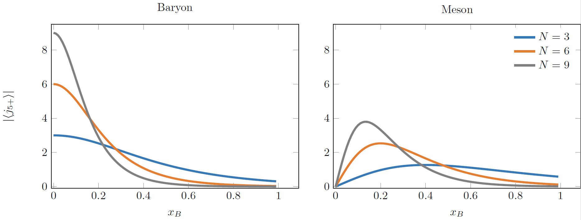
Figure 1: Left panel: The matrix element of the axial current inside a baryon as a function of Bjorken $x$ for different numbers of colors $N$. For large $N$, the $x_{B}\sim 1$ region is suppressed while the $x_{B}\rightarrow 0$ region is enhanced. Right panel: Same as left panel, but for a meson. The $x_{B}\rightarrow 0$ region contribution vanishes, reflecting the lack of baryon topology.

This behavior at low $x_{B}$ can be understood as arising from the nontrivial topology of the baryon. We can show this explicitly by considering the decomposition of our soliton state (37) into an energy component and a topological component. Rewriting it in the infinite momentum frame, we have

$$\phi_{b}(x^{+})=\sqrt{\frac{N}{\pi}}(\text{sign}\ast\text{sech})\left(\frac{\pi p_{+}x^{+}}{2N}\right)\ .$$ (46)

To mimic the meson wave function, we remove the baryon topology by replacing the sign function by a $\delta$-function and consider only the energy part

$$\phi_{b}^{n-t}(x^{+})=\sqrt{\frac{N}{\pi}}\frac{1}{\cosh\left(\frac{\pi p_{+}x^{+}}{2N}\right)}\ .$$ (47)

Of course, this solution is not a classical solution of the equation of motion; it is meant to provide a caricature of the meson wave function that does not possess the baryon topology.

Going through the steps outlined above, we find the axial current in the coherent state corresponding to this nontopological “mesonic” soliton:

$$\langle nontop.|j_{5+}(x_{B})|nontop.\rangle(x_{B})=\frac{2N^{2}x_{B}i}{\pi\cosh(Nx_{B})}.$$ (48)

We see that at small $x_{B}$ this expression vanishes, in stark contrast to the case of the baryon. Comparing the left and right panels of Fig. 1, we clearly see that the $x_{B}\rightarrow 0$ region contains only the topological contribution. The energy contribution vanishes at small $x_{B}$.

IV Discussion

In the traditional parton model, parton distributions are sensitive to the nonperturbative hadron structure only through the initial conditions for the evolution equations. The perturbative QCD evolution is then completely decoupled from the hadron structure, and is identical for baryons and mesons. There is, however, an important question about the role of nonperturbative effects, and in particular the effect of baryon topology on parton distributions. Addressing this question is very hard in real $(3+1)$-dimensional QCD, but we have solved the problem of parton distributions inside baryons exactly using ${\rm QCD}_{2}$ in the ’t Hooft limit.

In this limit, ${\rm QCD}_{2}$ reduces to the interacting sine-Gordon model. As we saw in the previous section, its topological solitons are dual to baryons. Moreover, they can be realized as quantum coherent states. We have evaluated the matrix element of the axial current on such states on the light cone. The soliton wave function can be exactly decomposed in a convolution of a topological and a nontopological contribution. We have shown that the main contribution (at leading order in $1/N$, where $N$ is the number of colors) to the “baryon” expectation value of $j_{5+}(x_{B})$ comes from the region $x_{B}<\frac{1}{N}$. We have also explicitly demonstrated that this enhancement at $x_{B}=0$ originates from the topology of the soliton.

These results provide new insights on the baryon structure at large $N$. Even though they have been obtained through bosonization, they are consistent with the picture of $N$ quarks moving in a mean field created by weak $\sim 1/N$ binary potentials, with $N^{2}$ quark pairs contributing to the average Hartree potential [12]. We find that this picture describes not only the mass of baryons at large $N$, but also their chirality distributions – namely, each quark carries $\sim 1/N$ fraction of the baryon’s chirality. Our results illustrate how the constituent quark picture of the baryon reemerges and is tied to the topological features of the bosonized solitonic solution.

One may wonder whether our results obtained in QCD₂ are relevant in the real $(3+1)$-dimensional world. The potential relevance of these results for spin physics follows from the operator product expansion (OPE) (60) that relates the hadronic tensor in polarized DIS to the expectation value of the axial current. However, the relation (19) between the axial and vector currents that locks the axial current to the vector charge, and many of the derivations in Section III linking the matrix element of the axial current to the topology of the baryon, are specific to $(1+1)$-dimensional theory. Nevertheless, we believe that our results may be relevant for the real QCD, for the following reasons. First, in (3+1) dimensions, there is also a linking of the UV and IR regions, through the chiral anomaly, with a corresponding anomaly matching; this is reminiscent of the anomaly matching in eqs. (9) and (10). Because of this, the polarized structure functions, even at large momentum transfer, are sensitive to the IR description of the hadron, and thus to its topology. Second, at high energies the transverse and longitudinal degrees of freedom factorize, so our $(1+1)$-dimensional treatment may be more relevant for high-energy interactions in the $(3+1)$-dimensional world than naively expected. One of the big differences between QCD₂ and QCD₄ is the absence of dynamical gluons in QCD₂. In the real $(3+1)$-dimensional QCD, the dynamical gluons are known to contribute to the polarized structure functions via the chiral anomaly [30, 31] that links the short and large distances [32]. As a result, the matrix element of the axial current measured in DIS becomes sensitive to the large distance, nonperturbative hadron structure [19, 18, 33, 20, 21, 22]. How would the topological structure of the baryon affect the gluon distributions in QCD₄? One possible mechanism is offered by the presence of “baryon junctions” in the wave functions of the baryons that are required by the gauge invariance [34]. These junctions have been found to provide an efficient non-perturbative mechanism for baryon stopping [35], but their implications for the polarized gluon distributions were never studied.

What are the phenomenological consequences of our results? Our main prediction is the dramatic difference between the spin distributions inside baryons and mesons. Since the singlet axial current contributes to the polarized structure function $g_{1}(x_{B})$, we expect that this structure function at small $x_{B}$ is enhanced for baryons and suppressed for mesons. This prediction can be tested in experiments, since meson structure functions can be accessed through the diffractive DIS with a baryon in the target fragmentation region separated by a rapidity gap from the inelastic final state. The polarized structure functions of baryons and mesons can also be measured in lattice QCD (see e.g. [36, 37, 38, 39, 40]).

Another interesting direction is suggested by the Gribov-Lipatov reciprocity relation [41] between the fragmentation functions and parton distributions. For quark fragmentation to protons, the corresponding fragmentation function $D_{p/q}(z)$ is softer than for mesons [42]. Through the reciprocity relation, this implies a softer quark distribution in Bjorken $x$ inside the proton, in accord with our findings. It would be interesting to extend the present study to spin-dependent quark fragmentation functions $\Delta D_{p/q}(z)$ into protons and vector mesons in semi-inclusive DIS.

Recently, the relation between the parton model and the hadron structure has been reexamined from the viewpoint of quantum information. Namely, the parton distributions were argued to arise from the reduced density matrix obtained from the pure density matrix of the hadron by tracing over the degrees of freedom that are unobservable in DIS. This approach predicts the emergence of the maximally entangled state at small $x$ [43, 44, 45] that can be viewed as an alternate picture of saturation [46, 47, 48] and is supported by the recent analyses [49, 50] of the DIS data from HERA [51]. From this viewpoint, the present work can be viewed as a first step in the extension of this approach to polarized structure functions, where the chiral anomaly plays a crucial role. It would be interesting to extend our study by explicitly evaluating the entanglement entropy and exploring its relation to the polarized structure functions. Another future direction would be to try and extend our approach to the $(3+1)$-dimensional QCD on the light cone; one way to proceed would be to use the $N_{f}=1$ baryon model proposed in [52]. Within QCD₂, it would be interesting to study the effect of $1/N$ corrections, and consider the theory with several quark flavors.

Appendix A Proton spin

This appendix contains a brief overview of the proton spin problem and its connection to gauge field topology, and the ways in which the proton spin distributions are measured in polarized deep inelastic scattering. Our notations follow [2].

The “proton spin” measured in DIS experiments is defined through the matrix element of the axial vector current:

$$2Ms^{\mu}=\langle\mathrm{p},s|\bar{\Pi}\gamma^{\mu}\gamma^{5}\Pi|\mathrm{p},s\rangle\ ,$$ (49)

where $|p,s\rangle$ is the proton state with spin $s$ and $\Pi$ is the fermionic proton operator; see also [53] for a more detailed discussion. In the experiment with polarized particles, a nonvanishing matrix element of the axial current manifests itself through the cross section dependence on polarization. The process most studied in this context is polarized deep inelastic scattering ${\vec{l}}+{\vec{\mathrm{p}}}\to{\vec{l}}+X$, where ${\vec{l}}$ is a polarized lepton and $X$ represents the sum over all possible channels. The corresponding cross section depends both on the polarization of the proton and of the initial lepton.

(a) Deep inelastic scattering.

(b) The photon-parton interaction vertex. $\xi\in[0,1]$ is the momentum fraction of the parton.

Figure 2:  

The leading contribution to DIS is shown in Fig. 2a. Given an incoming lepton with four-momentum $k$ and energy $E$ in the target rest frame, scattering off a hadron of mass $M$ with a momentum transfer $q=k-k^{\prime}$ and energy loss $\nu=E-E^{\prime}$, with $k^{\prime}$ and $E^{\prime}$ the four-momentum and energy of the outgoing lepton, one can define dimensionless Bjorken $x$ and inelasticity $y$ as

$$x_{B} =\frac{Q^{2}}{2M\nu}=\frac{Q^{2}}{2p\cdot q}\ ,$$ (50)

$$y =\frac{\nu}{E}\ ,$$ (51)

with $Q^{2}=-q^{2}$. The corresponding differential cross section can be expressed in terms of the leptonic and hadronic tensors, $l_{\mu\nu}$ and $W_{\mu\nu}$ (to be defined below), as

$$\frac{\mathrm{d}^{2}\sigma}{\mathrm{d}x_{B}\mathrm{d}y\mathrm{d}\phi}=\frac{e^{4}}{16\pi^{2}Q^{4}}l_{\mu\nu}W^{\mu\nu}_{\lambda\lambda}\ ,$$ (52)

where $\phi$ is the azimuthal angle of the scattered lepton.

The leptonic and hadronic tensors are defined in terms of the correlation functions of the electromagnetic current $j^{\mu}$ by computing the diagram 2a ( see [2] for a detailed derivation):

$$l^{\mu\nu} =\sum_{s_{f}}\langle k^{\prime},s_{f}|j^{\nu}_{l}(0)|k,s_{l}\rangle\langle k,s_{l}|j_{l}^{\mu}(0)|k^{\prime},s_{f}\rangle$$ (53)

$$W^{\mu\nu}_{\lambda\lambda^{\prime}} =\frac{1}{4\pi}\int\mathrm{d}^{4}xe^{iqx}\langle\mathrm{p},\lambda^{\prime}|[j^{\mu}(x),j^{\nu}(0)]|\mathrm{p},\lambda\rangle\ .$$ (54)

This decomposition fully splits the electromagnetic sector contribution from the QCD contribution. The tensor $l^{\mu\nu}$ can be directly computed in perturbation theory. On the other hand, the hadronic tensor $W^{\mu\nu}_{\lambda\lambda^{\prime}}$ is difficult to evaluate because of the nonperturbative nature of the strong interaction. To study it further, it is useful to decompose the hadronic tensor into an irreducible set of Lorentz structures, the so-called structure functions. In order to proceed, we first need to specify the polarization of the target proton. The most general polarization state for a spin $1/2$ target in its rest frame can be described by the following density matrix

$$\rho=\sum_{\lambda,\lambda^{\prime}=-1/2}^{1/2}A_{\lambda\lambda^{\prime}}|\lambda\rangle\langle\lambda^{\prime}|\ .$$ (55)

In this case, it is convenient to write the matrix $A$ in terms of Pauli operators

$$A=\frac{1}{2}\left(\mathbf{1}+\frac{1}{M}\vec{s}_{H}\cdot\vec{\sigma}\right)\ ,$$ (56)

where we used the fact that $\mathrm{Tr}(A)=1$ and the factor of $M$ is introduced for dimensional reasons.

The relation between the four-vector $s_{\mu}$ in (49) and $\vec{s}_{H}$ is established in the rest frame of the target through $s_{\mu}=(0,\frac{\vec{s}_{H}}{M})$; the polarization of the target is fully determined by this quantity. Assuming the polarization of the hadron is fixed, the hadronic tensor of interest becomes

$$W^{\mu\nu}=\sum_{\lambda\lambda^{\prime}}A_{\lambda\lambda^{\prime}}W^{\mu\nu}_{\lambda\lambda^{\prime}}\ .$$ (57)

We are now ready to define the structure functions. Taking into account current conservation $q_{\mu}W^{\mu\nu}=q_{\nu}W^{\mu\nu}=0$ together with the transformation properties of $W^{\mu\nu}$ under time reversal and parity transformations (which are derived from (54), see for instance [2]), the most general Lorentz covariant hadronic tensor for deep inelastic scattering on a polarized spin $1/2$ target is

$$W^{\mu\nu} =\left(-\eta_{\mu\nu}+\frac{q_{\mu}q_{\nu}}{q^{2}}\right)F_{1}+\frac{1}{p\cdot q}\left(p_{\mu}-\frac{p\cdot qq_{\mu}}{q^{2}}\right)\left(p_{\nu}-\frac{p\cdot qq_{\nu}}{q^{2}}\right)F_{2}$$

$$+\frac{i}{p\cdot q}\epsilon_{\mu\nu\rho\sigma}q^{\rho}s^{\sigma}g_{1}+\frac{i}{(p\cdot q)^{2}}\epsilon_{\mu\nu\rho\sigma}q^{\rho}\left(p\cdot qs^{\sigma}-s\cdot qp^{\sigma}\right)g_{2}\ .$$ (58)

The functions $F_{1},F_{2},g_{1},g_{2}$ are called the structure functions. They depend on the relativistic invariants $p^{2}=M^{2},p\cdot q,Q^{2}=-q^{2}$. It is conventional to express this dependence in terms of $Q^{2}$ and the dimensionless variable $x_{B}$. The functions $g_{1}$ and $g_{2}$ are sensitive to the polarization of the target and are often referred to as polarized structure functions.

When considering high energies and large momentum transfers, a particularly useful tool is the operator product expansion (OPE), which allows one to represent two point correlators, such as $W^{\mu\nu}$, as an expansion in local operators. The power counting for the expansion of $W^{\mu\nu}$ is done in terms of the “twist” of a given operator

$$t=\mathrm{dimension-spin}$$ (59)

and the leading order are twist two operators. In particular, the OPE allows us to understand the different structure functions in terms of contributions from local operators. In particular, at leading order, the part of the operator expansion of $W_{\mu\nu}$ contributing to $g_{1}$ (i.e. with the appropriate symmetries) is [53]

$$W^{\mu\nu}\underset{\begin{subarray}{c}Q^{2}\to\infty\end{subarray}}{\sim}2\epsilon^{\mu\nu\lambda\rho}\frac{p_{\lambda}}{Q^{2}}\left[C^{NS}\left(j_{\rho 5}^{3}+\frac{1}{\sqrt{3}}j_{\rho 5}^{8}\right)+\frac{2\sqrt{2}}{\sqrt{3}}C^{S}j^{0}_{\rho 5}\right]\ ,$$ (60)

where $j_{\mu 5}^{a}=\bar{q}\gamma_{\mu}\gamma_{5}T^{a}q$ is the QCD axial current with $T^{a}$ ($a=1,...,8$) being the generators of $SU(3)$, normalized so that $\text{Tr}\left(T^{a}T^{b}\right)=\frac{1}{2}\delta^{ab}$; $T^{0}=1/\sqrt{6}$. $C^{NS}$ and $C^{S}$ are Wilson coefficients which can be computed in perturbation theory. This relation provides a direct link between the structure function $g_{1}$ and the miscroscopic QCD axial current. In other words, measurements of $g_{1}$ can be interpreted as probing the axial charge content of the proton. This is also why measurements of $g_{1}$ are often referred to as probing the spin structure of the proton, as for free fields the axial charge is related to spin.

So far the discussion has been generic. We will now restrict ourselves to a particularly interesting limit in which DIS is often considered, the so-called Bjorken limit. In this case, the momentum transfer $Q^{2}$ is sent to infinity while keeping $x_{B}$ fixed. Asymptotic freedom then suggests that the physics can be described in terms of free quarks and gluons. This results in the structure functions depending only on $x_{B}$, a phenomenon known as “Bjorken scaling”. This is indeed the case at leading order, and the OPE and other perturbative QCD methods can be used to systematically compute corrections. Scaling, taken literally, leads to the “naive parton model”, where DIS cross sections are computed by considering a lepton scattering off a quark which carries a momentum fraction $\xi$ of the proton.

The parton model is usually formulated in a frame where the target nucleon has infinite momentum, the so-called infinite momentum frame (IMF). In this frame the target mass can be neglected, so that the nucleon has 4-momentum (assuming that it moves in the $z$-direction) $p^{\mu}=(p,0,0,p)$ and the parton has exactly a fraction $\xi$ of this momentum: $(\xi p,0,0,\xi p)$. By computing the scattering of a virtual photon and a free quark, represented in figure 2b (see for instance [2]), one can easily find the contribution of a single quark with momentum fraction $\xi$ to the distribution functions

$$F^{q,\xi}_{1}(x_{B}) =\frac{e_{q}^{2}}{2}\delta(\xi-x_{B})$$ (61)

$$F^{q,\xi}_{2}(x_{B}) =x_{B}e_{q}^{2}\delta(\xi-x_{B})=2x_{B}F^{q,\xi}_{1}(x_{B})$$ (62)

$$g^{q,\xi}_{1}(x_{B}) =\frac{e_{q}^{2}}{2}h_{q}h_{H}\delta(\xi-x_{B})$$ (63)

$$g^{q,\xi}_{2}(x_{B}) =0\ ,$$ (64)

where $e_{q}$ is the electric charge of the quark and $h_{q}$ is the helicity of the free quark. The quantity $h_{H}$ denotes the helicity of the target; in the IMF polarization of the target becomes $s_{H}=ph_{H}$. In this picture, the structure functions acquire an intuitive meaning. Defining $q_{\pm}(\xi)$ as being the probability distribution of a quark whose helicity is aligned/antialigned to the proton’s, integrating over the momentum fraction $\xi$ and summing over helicities, we obtain

$$F^{part.\ mod.}_{1}(x_{B}) =\sum_{q}\frac{e_{q}^{2}}{2}\left(q_{+}(x_{B})+q_{-}(x_{B})+\bar{q}_{+}(x_{B})+\bar{q}_{-}(x_{B})\right)$$ (65)

$$F^{part.\ mod.}_{2}(x_{B}) =2xF_{1}(x_{B})$$ (66)

$$g^{part.\ mod.}_{1}(x_{B}) =\sum_{q}\frac{e_{q}^{2}}{2}\left(q_{+}(x_{B})-q_{-}(x_{B})+\bar{q}_{+}(x_{B})-\bar{q}_{-}(x_{B})\right)$$ (67)

$$g^{part.\ mod.}_{2}(x_{B}) =0\ .$$ (68)

We see that in the Bjorken limit, $x_{B}$ can be interpreted as the momentum fraction of a proton that a constituent parton is carrying in the infinite momentum frame. The function $F_{1}(x_{B})$ is then simply the probability distribution of finding a given quark in the hadron with momentum fraction $x_{B}$. The function $g_{1}(x_{B})$ measures polarization asymmetries in the quark distributions.

The integral of $g_{1}$ over $x_{B}$ yields its first Mellin moment; plugging in the quark charges, we get

$$\int\mathrm{d}x_{B}g^{part.\ mod.}_{1}(x_{B}) =\frac{1}{2}\left[\frac{4}{9}\Delta u+\frac{1}{9}\Delta d+\frac{1}{9}\Delta s\right],$$ (69)

where we have defined $\Delta q=\int\mathrm{d}x_{B}\left(q_{+}(x_{B})-q_{-}(x_{B})\right)$. It is useful to further rewrite it in terms of axial currents that appear in eq. (60). The axial charges are defined as

$$2Ms^{\mu}g_{A}^{(a)}=\langle\mathrm{p},s|j_{5}^{\mu(a)}|\mathrm{p},s\rangle.$$ (70)

A frequently used convention is to reabsorb some of the $SU(3)$ normalization into the axial charges by defining [53]

$$a^{3}=2g_{A}^{3},\ \ \ \ a^{8}=2\sqrt{3}g_{A}^{8},\ \ \ \ a^{0}=\sqrt{6}g_{A}^{0}\ .$$ (71)

In these terms, the parton model prediction for the first moment of $g_{1}$ yields the Ellis-Jaffe sum rule

$$\int_{0}^{1}\mathrm{d}x_{B}g_{1}(x_{B})=\frac{1}{12}a^{3}+\frac{1}{36}a^{8}+\frac{1}{9}a^{0}\ ,$$ (72)

where the axial charges $a^{3}$ and $a^{8}$ can be independently inferred from low-energy data on neutron $\beta$-decay and hyperon decay (assuming $SU(3)$ symmetry) [55]. Assuming the validity of the parton model, a measurement of the first moment of $g_{1}$ is effectively a measurement of the singlet axial charge $a^{0}=\Delta u+\Delta d+\Delta s$.

The measurements of polarization asymmetries in the final states in polarized DIS give a value of $a_{0}|_{Q^{2}\to\infty}=0.33\pm 0.06$ [53]. This value is in sharp contradiction with the value predicted by the constituent quark model. As reviewed in [5], the most naïve nonrelativistic $SU(6)$ description of the proton yields $a^{0}=1$. More realistic relativistic “bag” models predict $a^{0}\approx 0.6$, still leaving a discrepancy of a factor of 2.

A major ingredient which has been missing in our discussion so far is how the gluons contribute to the proton axial charge. In the partonic description, the gluons are absent from the picture. This can be traced back to the OPE for $g_{1}$ (60), where no gluonic operators are present at leading order. Indeed, the only gluonic operator of twist two is the topological charge density

$$Q(x)=\frac{\alpha_{s}}{4\pi}\text{Tr}\left(G_{\mu\nu}\tilde{G}^{\mu\nu}\right)$$ (73)

where $\alpha_{s}$ is the QCD coupling constant. As is well known, this operator is a total derivative

$$Q(x) =2\partial_{\mu}K^{\mu}$$ (74)

$$K_{\mu} =\frac{\alpha_{s}}{8\pi}\epsilon_{\mu\nu\lambda\rho}\left[A^{\nu}_{a}\left(\partial^{\lambda}A^{\rho}_{a}-\frac{1}{3}gf_{abc}A^{\lambda}_{b}A^{\rho}_{c}\right)\right]\ ,$$ (75)

and as a result does not contribute in perturbation theory. It is also well known that topological charge is precisely the operator that nonperturbatively leads to an anomalous nonconservation of the axial vector

$$\partial_{\mu}j_{5}^{\mu}=N_{f}Q(x)$$ (76)

where $N_{f}=3$ is the number of flavors. As a result the operator $Q(x)$ is expected to give a substantial nonperturbative contribution to the axial charge. To describe this effect, we can rewrite the anomaly equation (76) as

$$\partial_{\mu}(j_{5}^{\mu}-2N_{f}K^{\mu})=0\ .$$ (77)

This form suggests to introduce a similar decomposition for the axial charge. In particular, we decompose $a^{0}$ as

$$a^{0}=\tilde{a}^{0}-\frac{\alpha_{s}}{2\pi}N_{f}\Delta g\ ,$$ (78)

with $\Delta g$ an explicit contribution from the topological gluonic operator and $\tilde{a}^{0}$ the remainder of the proton axial charge.

This decomposition was suggested early on as a solution to the “spin” crisis [56, 57, 18, 19, 20], and recently revisited in [21, 22]. Indeed, as suggested by this decomposition, the topological gluonic configuration can potentially screen the axial charge inside the proton. In this scenario, one expects that $\tilde{a}_{0}$ corresponds to the net axial charge carried by quarks inside the proton, in accord with the naïve quark model.

References

- Roberts [1990] R. G. Roberts, The Structure of the Proton: Deep Inelastic Scattering, Cambridge Monographs on Mathematical Physics (Cambridge University Press, 1990).
- Manohar [1992] A. V. Manohar, in Lake Louise Winter Institute: Symmetry and Spin in the Standard Model (1992) arXiv:hep-ph/9204208 .
- Anselmino et al. [1995] M. Anselmino, A. Efremov, and E. Leader, Phys. Rept. 261, 1 (1995), [Erratum: Phys.Rept. 281, 399–400 (1997)], arXiv:hep-ph/9501369 .
- Filippone and Ji [2001] B. W. Filippone and X.-D. Ji, Adv. Nucl. Phys. 26, 1 (2001), arXiv:hep-ph/0101224 .
- Bass [2005] S. D. Bass, Rev. Mod. Phys. 77, 1257 (2005), arXiv:hep-ph/0411005 .
- Aidala et al. [2013] C. A. Aidala, S. D. Bass, D. Hasch, and G. K. Mallot, Rev. Mod. Phys. 85, 655 (2013), arXiv:1209.2803 [hep-ph] .
- ’t Hooft [1974a] G. ’t Hooft, Nucl. Phys. B 75, 461 (1974a).
- Witten [1984] E. Witten, Commun. Math. Phys. 92, 455 (1984).
- Frishman and Sonnenschein [1993] Y. Frishman and J. Sonnenschein, Phys. Rept. 223, 309 (1993), arXiv:hep-th/9207017 .
- Gross et al. [1996] D. J. Gross, I. R. Klebanov, A. V. Matytsin, and A. V. Smilga, Nucl. Phys. B 461, 109 (1996), arXiv:hep-th/9511104 .
- Skyrme [1962] T. H. R. Skyrme, Nucl. Phys. 31, 556 (1962).
- Witten [1979] E. Witten, Nucl. Phys. B 160, 57 (1979).
- Brodsky et al. [1988] S. J. Brodsky, J. R. Ellis, and M. Karliner, Phys. Lett. B 206, 309 (1988).
- Coleman [1975] S. R. Coleman, Phys. Rev. D 11, 2088 (1975).
- Faddeev and Korepin [1978] L. D. Faddeev and V. E. Korepin, Phys. Rept. 42, 1 (1978).
- Zamolodchikov and Zamolodchikov [1979] A. B. Zamolodchikov and A. B. Zamolodchikov, Annals Phys. 120, 253 (1979).
- Dvali et al. [2015] G. Dvali, C. Gomez, L. Gruending, and T. Rug, Nucl. Phys. B 901, 338 (2015), arXiv:1508.03074 [hep-th] .
- Hatsuda and Zahed [1989] T. Hatsuda and I. Zahed, Phys. Lett. B 221, 173 (1989).
- Jaffe and Manohar [1990] R. L. Jaffe and A. Manohar, Nucl. Phys. B 337, 509 (1990).
- Shore and Veneziano [1990] G. M. Shore and G. Veneziano, Phys. Lett. B 244, 75 (1990).
- Tarasov and Venugopalan [2020] A. Tarasov and R. Venugopalan, Phys. Rev. D 102, 114022 (2020), arXiv:2008.08104 [hep-ph] .
- Tarasov and Venugopalan [2022] A. Tarasov and R. Venugopalan, Phys. Rev. D 105, 014020 (2022), arXiv:2109.10370 [hep-ph] .
- Schwinger [1962] J. S. Schwinger, Phys. Rev. 128, 2425 (1962).
- Baluni [1980] V. Baluni, Phys. Lett. B 90, 407 (1980).
- Steinhardt [1980] P. J. Steinhardt, Nucl. Phys. B 176, 100 (1980).
- Zhitnitsky [1985] A. R. Zhitnitsky, Phys. Lett. B 165, 405 (1985).
- Abdalla and Abdalla [1996] E. Abdalla and M. C. B. Abdalla, Phys. Rept. 265, 253 (1996), arXiv:hep-th/9503002 .
- Anand et al. [2021] N. Anand, A. L. Fitzpatrick, E. Katz, and Y. Xin, (2021), arXiv:2111.00021 [hep-th] .
- Dashen et al. [1975] R. F. Dashen, B. Hasslacher, and A. Neveu, Phys. Rev. D 11, 3424 (1975).
- Adler [1969] S. L. Adler, Phys. Rev. 177, 2426 (1969).
- Bell and Jackiw [1969] J. S. Bell and R. Jackiw, Nuovo Cim. A 60, 47 (1969).
- Dolgov and Zakharov [1971] A. D. Dolgov and V. I. Zakharov, Nucl. Phys. B 27, 525 (1971).
- Efremov et al. [1990] A. V. Efremov, J. Soffer, and O. V. Teryaev, Nucl. Phys. B 346, 97 (1990).
- Rossi and Veneziano [1977] G. C. Rossi and G. Veneziano, Nucl. Phys. B 123, 507 (1977).
- Kharzeev [1996] D. Kharzeev, Phys. Lett. B 378, 238 (1996), arXiv:nucl-th/9602027 .
- Göckeler et al. [1996] M. Göckeler, R. Horsley, E.-M. Ilgenfritz, H. Perlt, P. Rakow, G. Schierholz, and A. Schiller, Physical Review D 53, 2317 (1996).
- Best et al. [1997] C. Best, M. Göckeler, R. Horsley, E.-M. Ilgenfritz, H. Perlt, P. Rakow, A. Schäfer, G. Schierholz, A. Schiller, and S. Schramm, Physical Review D 56, 2743 (1997).
- Green et al. [2014] J. Green, M. Engelhardt, S. Krieg, J. Negele, A. Pochinsky, and S. Syritsyn, Physics Letters B 734, 290 (2014).
- Chen et al. [2016] J.-W. Chen, S. D. Cohen, X. Ji, H.-W. Lin, and J.-H. Zhang, Nuclear Physics B 911, 246 (2016).
- Lin et al. [2018] H.-W. Lin, E. R. Nocera, F. Olness, K. Orginos, J. Rojo, A. Accardi, C. Alexandrou, A. Bacchetta, G. Bozzi, J.-W. Chen, et al., Progress in Particle and Nuclear Physics 100, 107 (2018).
- Gribov and Lipatov [1971] V. Gribov and L. Lipatov, Physics Letters B 37, 78 (1971).
- Group et al. [2020] P. D. Group, P. Zyla, R. Barnett, J. Beringer, O. Dahl, D. Dwyer, D. Groom, C.-J. Lin, K. Lugovsky, E. Pianori, et al., Progress of Theoretical and Experimental Physics 2020, 083C01 (2020).
- Kharzeev and Levin [2017] D. E. Kharzeev and E. M. Levin, Phys. Rev. D 95, 114008 (2017), arXiv:1702.03489 [hep-ph] .
- Kharzeev [2021] D. E. Kharzeev, Phil. Trans. A. Math. Phys. Eng. Sci. 380, 20210063 (2021), arXiv:2108.08792 [hep-ph] .
- Zhang et al. [2022] K. Zhang, K. Hao, D. Kharzeev, and V. Korepin, Phys. Rev. D 105, 014002 (2022), arXiv:2110.04881 [quant-ph] .
- Dvali and Venugopalan [2022] G. Dvali and R. Venugopalan, Phys. Rev. D 105, 056026 (2022), arXiv:2106.11989 [hep-th] .
- Liu et al. [2022a] Y. Liu, M. A. Nowak, and I. Zahed, (2022a), Phys. Rev. D 105, 114027 (2022), arXiv:2202.02612 [hep-ph] .
- Liu et al. [2022b] Y. Liu, M. A. Nowak, and I. Zahed, (2022b), Phys. Rev. D 105, 114028 (2022), arXiv:2203.00739 [hep-ph] .
- Kharzeev and Levin [2021] D. E. Kharzeev and E. Levin, Phys. Rev. D 104, L031503 (2021), arXiv:2102.09773 [hep-ph] .
- Hentschinski and Kutak [2022] M. Hentschinski and K. Kutak, Eur. Phys. J. C 82, 111 (2022), arXiv:2110.06156 [hep-ph] .
- Andreev et al. [2021] V. Andreev et al. (H1), Eur. Phys. J. C 81, 212 (2021), arXiv:2011.01812 [hep-ex] .
- Komargodski [2018] Z. Komargodski, (2018), arXiv:1812.09253 [hep-th] .
- Shore [2008] G. M. Shore, Lect. Notes Phys. 737, 235 (2008), arXiv:hep-ph/0701171 .
- Sterman [1995] G. F. Sterman, in Theoretical Advanced Study Institute in Elementary Particle Physics (TASI 95): QCD and Beyond (1995) pp. 327–408, arXiv:hep-ph/9606312 .
- Ellis and Jaffe [1974] J. R. Ellis and R. L. Jaffe, Phys. Rev. D 9, 1444 (1974), [Erratum: Phys.Rev.D 10, 1669 (1974)].
- Carlitz et al. [1988] R. D. Carlitz, J. C. Collins, and A. H. Mueller, Phys. Lett. B 214, 229 (1988).
- Altarelli and Ross [1988] G. Altarelli and G. G. Ross, Phys. Lett. B 212, 391 (1988).