Dynamical relaxation of cosmological constant

Abstract

A special class of conformal gravity theories is proposed to solve the long standing problem of the fine-tuned cosmological constant. In the proposed model time evolution of the inflaton field leaves behind a nearly vanishing, but finite value of dark energy density of order (a few meV)⁴ to explain the late-time accelerating universe. A multiple scalar inflaton field is assumed to have a conformal coupling to the Ricci scalar curvature in the lagrantian, which results in, after a Weyl rescaling to the Einstein metric frame, modification of inflaton kinetic and potential terms along with its coupling to Higgs fields in the standard model. One may define an effective cosmological $\Lambda$ function in the Einstein metric frame, which controls, when the potential is added, a slow-roll inflation and subsequent oscillation at the potential minimum of a spontaneous symmetry breaking phase. The inflaton oscillation accompanies particle production towards thermalized hot big-bang universe. At the same time zero-point quantum fluctuation of second inflaton field is generated, and its accumulated fluctuation gives rise to a symmetry restoration, pushing back the inflaton field towards the infinity. This gives a dynamical relaxation of vanishing effective cosmological constant. Both inhomogeneous inflaton modes and their collapsed black holes of primordial origin are good candidates of cold dark matter.

I Introduction

There exist a vast literature of proposals, [1], [2], [3], [4], [5], to resolve the fine-tuned cosmological constant problem. We would like to add a new idea to this list. If our idea is correct, it requires a flesh view of the early universe, as explained in the present and subsequent works.

We need to combine a few concepts in order to construct our framework, hence we first explain how they come about.

(1) In order to regard the cosmological constant as dynamical, we introduce conformal coupling to the Ricci scalar curvature $R$ in the form, $-M_{\rm P}^{2}F(\chi)R$, in the lagrangian density. Here $\chi$ is the inflaton field and $M_{\rm P}\approx 10^{18}$GeV is the Planck energy. After the Weyl rescaling of the metric tensor to eliminate $F(\chi)$, the cosmological constant $\Lambda$ is changed to a functional variable $\Lambda_{\rm eff}=\Lambda/F^{2}(\chi)$. With a choice of appropriate polynomial for $F(\chi)$, this dynamical cosmological constant becomes null at $\chi\rightarrow\infty$.

(2) Slow-roll inflation is realized giving a right amount of spectral index and tensor-to-scalar mode ratio consistent with observations. Inflation ends with Higgs boson production followed by quick thermalization among standard model particles by their coupling to Higgs boson. The particle production is described as a parametric amplification of time dependent harmonic oscillator system. Besides interaction term of the form, $\chi^{2}H^{2}$ to the Higgs boson $H$, the inflaton $\chi$ also couples to another scalar field $\phi$. $\chi$ field oscillation occurs around a potential minimum of $V(\chi)$ away from the origin at $\chi=0$ in which Nambu-Goldstone kinetic repulsion dominates [6]. It is driven by a Higgs-like potential $V(\chi)=g(\chi^{2}+\phi^{2}-v^{2})^{2}/4\,,g>0$. $\phi$ production is necessarily accompanied by quantum zero-point fluctuation $\langle\phi^{2}\rangle$. This induces a positive contribution to $\chi$ mass like $g\langle\phi^{2}\rangle$, adding to the original negative term $-gv^{2}\equiv-m_{\chi}^{2}<0$.

(3) The leading behavior of the effective potential contains a piece $(-m_{\chi}^{2}+g\langle\phi^{2}\rangle)/\chi^{2}$. Hence the potential minimum disappears at a critical point, $g\langle\phi^{2}\rangle=m_{\chi}^{2}$, signaling a kind of phase transition. Some time after this critical fluctuation is reached, the $\chi$ field leave the potential minimum, and rolls to the field infinity governed by $-\ln\chi$ potential, giving essentially the vanishing cosmological constant.

(4) Spatially homogeneous part constitutes dark energy whose energy density at present becomes of order $(H_{0}M_{\rm P})^{2}\sim({\rm a\;few\;meV})^{4}$. At the same time field quanta of inhomogeneous modes are thermally produced from ambient medium, and shortly after the electroweak phase transition they behave as non-relativistic cold dark matter (CDM). Gravitationally collapsed clumps of inhomogeneous modes are another good candidate of cold dark matter.

The rest of this paper is organized as shown in the following table of contents.

=============================

II. Conformal coupling to gravity and dynamical cosmological “constant”

A. Conformal gravity

B. Choice of conformal coupling function and potential

C. Spontaneous symmetry breaking and Nambu-Goldstone kinetic modes

D. Inflaton coupling to Higgs boson

III. Time evolution at inflationary epoch

A. Field and Einstein equations

B. Slow-roll inflation

C. Spectral index and tensor-to-scalar ratio

D. Oscillation at the end of inflation

IV. Particle production and symmetry restoration

A. Particle production and quantum fluctuation due to inflaton oscillation

B. Radiation dominated epoch

V. Late time acceleration

A. Differential equations and its solutions

B. Equation-of-state factor

VI. Inhomogeneous inflaton modes and candidate cold dark matter

A. Inhomogeneous inflaton modes

B. Time variation of CDM energy density

VII. Summary

VIII. Appendix: Production rate and decay freeze-out of inhomogeneous inflaton modes

============================= We use the natural unit of $\hbar=c=1$ and the Boltzmann constant $k_{B}=1$ throughout the present work unless otherwise stated. The cosmic scale factor $a(t)$ is introduced in the flat Friedman-Robertson-Walker metric, $ds^{2}=dt^{2}-a^{2}(t)(d\vec{x})^{2}$ [7].

II Conformal coupling to gravity and dynamical cosmological “constant”

II.1 Conformal gravity

We would like to treat the cosmological constant $\Lambda$ as a dynamical variable $\Lambda_{\rm eff}(t)$. Let us explore for this purpose conformal coupling to gravity in which $\Lambda$ term is multiplied by a function of inflaton field after a Weyl rescaling.

The simplest conformal gravity scheme uses a single real inflaton field $\chi$, and the next simplest scheme for our purpose uses two complex fields, the inflaton and an additional scalar field $\phi$. In this subsection we shall deal with the first case. In the Jordan metric frame [8] the lagrangian density has a generic form,

$${\cal L}={\cal L}_{\chi g}^{(J)}+{\cal L}_{\rm SM}\,,\hskip 14.22636pt{\cal L}_{\chi g}^{(J)}=\sqrt{-g}\times$$

$$\left(-M_{\rm P}^{2}F(\chi)R(g_{\mu\nu})-2M_{\rm P}^{2}\,\Lambda+\frac{1}{2}(\partial\chi)^{2}-V(\chi)\right)\,,$$ (1)

$${\cal L}_{\rm SM}=\sqrt{-g}L_{\rm SM}(\psi,g_{\mu\nu})\,,$$ (2)

$$M_{\rm P}^{2}=\frac{1}{16\pi G_{N}}\sim(1.72\times 10^{18}\,{\rm GeV})^{2}\,,\hskip 14.22636pt\Lambda>0\,.$$ (3)

$L_{\rm SM}(\psi,g_{\mu\nu})$ is the standard model lagrangian density with $\psi$ fields of standard theory; gauge bosons, Higgs boson, and fermions (quarks and leptons), generically. There are two functional degrees of freedom; $F(\chi)$ and $V(\chi)$ in the scalar-tensor gravity given by ${\cal L}_{\chi g}^{(J)}$. These are called the conformal couping function and the potential function. We restrict these to polynomial forms, and assume a reflection symmetry $F(-\chi)=F(\chi)$ and $V(-\chi)=V(\chi)$, hence they are even polynomial functions of $\chi^{2}$. The Jordan frame is useful if four dimensional conformal gravity descends from higher dimensional theories such as Kaluza-Klein unification [9], [10] and superstring theories.

It is physically more transparent in cosmological applications to transform the lagrangian density in the Jordan frame to that in the Einstein metric frame by a Weyl-rescaling, $\bar{g}_{\mu\nu}=F(\chi)g_{\mu\nu}$. To simplify our notation, we replace the new metric $\bar{g}_{\mu\nu}$ by $g_{\mu\nu}$. The lagrangian density in the new Einstein frame is then

$${\cal L}_{\chi g}^{(E)}=\sqrt{-g}\left(-M_{\rm P}^{2}R(g_{\mu\nu})+\frac{5}{2F(\chi)}(\partial\chi)^{2}\right.$$

$$\left.-\frac{1}{F^{2}(\chi)}(2M_{\rm P}^{2}\,\Lambda+V(\chi)\right)\,.$$ (4)

The metric is transformed as well according to $ds^{2}=F^{-1}(dt^{2}-a^{2}(d\vec{x})^{2})$. One can re-define field variable to $\bar{\chi}$, though not necessary, to obtain the standard, normalized form of kinetic term, $5(\partial\chi)^{2}/(2F)=(\partial\bar{\chi})^{2}/2$, leaving a complicated potential function. But we keep the original form above.

We may define a dynamical cosmological variable $\Lambda_{\rm eff}(\chi)$ by

$$V_{\chi g}^{(E)}=2M_{\rm P}^{2}\Lambda_{\rm eff}(\chi)+\frac{V(\chi)}{F^{2}(\chi)}\,,$$ (5)

$$\Lambda_{\rm eff}(\chi)=\frac{\Lambda}{F^{2}(\chi)}\,.$$ (6)

which appears in (4). It should be clear that $\Lambda_{\rm eff}(\chi)$, and not $\Lambda$, should vanish when the problem of cosmological constant is solved. It is found later that cosmological evolution drives $\chi$ towards the infinity. It is then clear that the maximum power of polynomial ratio $V(\chi)/F^{2}(\chi)$ becomes important. Suppose that the maximum powers of the two functions, $V\,,F$ are $2n$ and $2l$ such that $V(\chi)/F^{2}(\chi)\rightarrow\chi^{2n-4l}$. It is found that $l=n$ case gives a positive force term $\propto 1/\chi$ to the inflaton field equation, and a dynamical cosmological constant $\propto 1/\chi^{2l}$. We shall work out most extensively the case of $l=n=2$, quartic conformal and potential functions denoted by $(F_{4},V_{4})$.

II.2 Choice of conformal coupling function and potential

We parametrize the conformal coupling function and the potential as

$$V=V_{4}(\chi)=-\frac{m_{\chi}^{2}}{2}\chi^{2}+\frac{g}{4}\chi^{4}\,,$$ (7)

$$F=F_{4}(\chi)=1+\xi_{2}(\frac{\chi}{M_{\rm P}})^{2}+\xi_{4}(\frac{\chi}{M_{\rm P}})^{4}\,.$$ (8)

We arranged parameters of $m_{\chi}^{2}>0$ such that a spontaneous breaking of a discrete symmetry occurs at $\chi^{2}=m_{\chi}^{2}/g$. All other constant parameters are taken positive.

It would be useful to record limiting behaviors of the effective cosmological constant $\Lambda_{\rm eff}(\chi)$ in the $(F_{4},V_{4})$ model, at small and large fields:

$$V_{\chi g}^{(E)}\rightarrow\Lambda-\frac{m_{\chi}^{2}+8\xi_{2}\Lambda}{4M_{\rm P}^{2}}\chi^{2}+O(\chi^{4})\,,\hskip 8.5359pt{\rm as}\;\chi\rightarrow 0\,,$$ (9)

$$V_{\chi g}^{(E)}\rightarrow\frac{g}{8\xi_{4}^{2}}\frac{M_{\rm P}^{6}}{\chi^{4}}+O(\chi^{-6})\,,\hskip 8.5359pt{\rm as}\;\chi\rightarrow\infty\,.$$ (10)

Note that the original cosmological constant disappears in the infinite field limit.

II.3 Spontaneous symmetry breaking and Nambu-Goldstone kinetic modes

So far we considered a discrete reflection symmetry of a real inflaton field. What is important in resolution of the cosmological constant problem is, however, a spontaneously broken continuous symmetry, which gives rise to Nambu-Goldstone modes. But if the inflaton field after inflation is permanently trapped in the potential minimum implied by the broken phase, there may exist an unacceptably large cosmological constant. To avoid this catastrophe, the potential minimum must change towards the vanishing effective cosmological constant at the field infinity. This is made possible if a higher continuous symmetry exists and a quantum fluctuation of another inflaton field develops such that symmetry restoration becomes possible. The simplest realization of this scenario is to choose O(4) symmetry breaking.

We shall start from the simplest O(2) symmetric model from a pedagogical reason. In two-component field space of $(\chi_{1},\chi_{2})$ an abstract angular momentum may be defined by $\chi^{2}\dot{\theta}$ where $(\chi_{1},\chi_{2})=\chi(\cos\theta\,,\sin\theta)$. The angular field equation of this inflaton system gives $\partial_{t}(a^{3}\chi^{2}\dot{\theta})=0$. This equation has a trivial solution; $\chi^{2}\dot{\theta}=c_{\chi}/a^{3}$ with $c_{\chi}$ a constant of integration. This solution may be incorporated as a centrifugal repulsion term in an effective potential, $c_{\chi}^{2}/(2a^{6}\chi^{2})$ [6].

In O(3) extension the invariant angular momentum operator is uniquely defined, and this single operator is not sufficient to ensure symmetry restoration for resolution of the cosmological constant problem. The next extension to O(4) symmetry introduces two invariant angular momenta, since this group is locally isomorphic to O₊(3) $\times$ O_-(3). The generators of this maximal subgroup are $(L_{41}\pm L_{23})/2\,,(L_{42}\pm L_{31})/2\,,(L_{43}\pm L_{12})/2$. Using four real inflaton fields, $\chi_{i}\,,i=1\sim 4$, one finds that two invariant squared fields denoted by $\chi^{2},\phi^{2}$ exist:

$$(\chi^{2}\,,\phi^{2})=3\sum_{i=1}^{4}\chi_{i}^{2}\pm 2(\chi_{1}\chi_{2}+\chi_{2}\chi_{3}+\chi_{3}\chi_{1})\,.$$ (11)

We shall assume $\chi^{2}>\phi^{2}$, calling them large and small components. Using these, one derives the centrifugal repulsive potential in O(4) symmetric model:

$$\frac{c_{+}^{2}}{2a^{6}\chi^{2}}+\frac{c_{-}^{2}}{2a^{6}\phi^{2}}\,.$$ (12)

Our new potential for two inflaton fields is, in the Jordan frame,

$$\hskip 28.45274ptV^{(J)}(\chi,\phi)=$$

$$\frac{c_{+}^{2}}{2a^{6}\chi^{2}}+\frac{c_{-}^{2}}{2a^{6}\phi^{2}}+\frac{g}{4}(\chi^{2}+\phi^{2}-\frac{m_{\chi}^{2}}{g})^{2}+2M_{\rm P}^{2}\Lambda\,.$$ (13)

The centrifugal repulsion acts as a potential wall at field zero, and its effect becomes important at late times.

II.4 Inflaton coupling to Higgs boson

An appealing feature of $F-$factor is that it automatically introduces inflaton coupling to standard model particles, in particular to the Higgs doublet $H$:

$$V_{H}^{(E)}=\frac{\lambda_{H}}{4}\,F^{-2}(|H|^{2}-v^{2})^{2}\,.$$ (14)

With extended two $(\chi,\phi)$ real fields of O(4) scheme a reduced O(2) symmetric field combination $\bar{\chi}^{2}=\chi^{2}+\phi^{2}$ appears in the variable function, $F(\bar{\chi}^{2})$. Both Higgs boson mass and inflaton coupling to Higgs boson are determined by eq.(14), and they are dynamical, meaning that these quantities are dependent on cosmic times, or the redshift factor $z+1=a(t_{0})/a(t)$.

We need to separate particle quantum field parts, $\chi\,,\phi$, from the c-number background field denoted by $\chi_{b}(t)$. This separation leads to

$$\bar{\chi}^{2}=\chi_{b}^{2}+2\chi_{b}\chi+\chi^{2}+\phi^{2}\,,\hskip 8.5359pt\chi_{b}\gg\sqrt{\chi^{2}+\phi^{2}}\,,$$ (15)

$$F^{-2}=\left(\xi_{4}\frac{\chi_{b}^{4}}{M_{\rm P}^{4}}\right)^{-2}\left(1-8\frac{\chi}{\chi_{b}}+O(\frac{\chi^{2}}{\chi_{b}^{2}}\,,\frac{\phi^{2}}{\chi_{b}^{2}})\right)\,.$$ (16)

The physical Higgs field $H_{0}$ is identified after the electroweak phase transition by $H=(H_{0}+v\,,0)$, the rest of doublet components being absorbed as longitudinal parts of electroweak gauge bosons. Hence, when the separation of inflaton field is applied to (14), the potential relevant to the Higgs boson mass is

$$m_{H}=125\,{\rm GeV}\,\left(\xi_{4}(\frac{\chi_{b}}{M_{\rm P}})^{4}\right)^{-1}\,.$$ (17)

The large field limit formula was used here. Note that the last factor in (17) is caused by the metric change due to $F$ entailing the spacetime coordinate change. This further modifies the unit change of energy and mass, hence it is not really a change of physical mass.

Three-point vertexes of $\chi\phi\phi\,,\chi H_{0}H_{0}$ are derived from the same equation (14);

$$V_{\chi\phi H}^{(E)}=c_{\phi}\chi\phi^{2}+c_{H}\chi H_{0}^{2}\,,$$ (18)

$$c_{\phi}=g\chi_{b}\,,\hskip 8.5359ptc_{H}=-8\lambda_{H}\frac{v^{2}}{\chi_{b}}(\xi_{4}\frac{\chi_{b}^{4}}{M_{\rm P}^{4}})^{-2}\,.$$ (19)

This lagrangian density can describe $\chi$ production processes via virtual Higgs-exchange diagram, $ll\rightarrow ll\chi\,,qq\rightarrow qq\chi$ with $l\,,q$ being leptons and quarks, and $\chi$ decay process, $\chi\rightarrow\phi\phi\,,\chi\rightarrow H_{0}H_{0}\,,H_{0}l\bar{l}\,,H_{0}q\bar{q}$, depending on the mutual mass relation between $\chi$ and $H_{0}$. Redshift dependence of background $\chi_{b}-$field shall be calculated to give production and decay rates in subsequent sections.

III Time evolution at inflationary epoch

III.1 Field and Einstein equations

For discussion of inflationary epoch only $\chi$ field is important, and we shall retain relevant parts alone. Thus, inflaton coupling to the Higgs field can be neglected.

The general form of the inflaton field equation is derived using the variational principle applied to ${\cal L}_{\chi g}^{(E)}$ of eq.(4):

$$5\left(\partial_{t}\frac{\partial_{t}\chi}{F(\chi)}+3\frac{\dot{a}}{a}\frac{\partial_{t}\chi}{F(\chi)}-\frac{1}{a^{2}}\vec{\nabla}\frac{\vec{\nabla}\chi}{F(\chi)}\right)=-\frac{\partial}{\partial\chi}V_{\chi g}^{(E)}(\chi)\,.$$

We shall first discuss the spatially homogeneous mode, assuming $\chi$ field depending on time alone. Using time derivative $d(1/F)/dt=-\dot{\chi}\partial_{\chi}F/F^{2}$, the field equation is

$$\ddot{\chi}+3\frac{\dot{a}}{a}\dot{\chi}-\frac{\partial_{\chi}F}{F}\dot{\chi}^{2}=-\frac{1}{5}F\,\frac{\partial}{\partial\chi}V_{\chi g}^{(E)}(\chi)\,,$$ (21)

$$F\,\frac{\partial}{\partial\chi}V_{\chi g}^{(E)}(\chi)=\frac{1}{F}\left(\partial_{\chi}V-2(V+2M_{\rm P}^{2}\Lambda)\frac{\partial_{\chi}F}{F}\right)\,.$$ (22)

In $(F_{4},V_{4})$ model, the leading asymptotic behavior of the right-hand side of field equation (21) is

$$\frac{g}{5\xi_{4}}\frac{M_{\rm P}^{4}}{\chi}+O(\chi^{-3})\,.$$ (23)

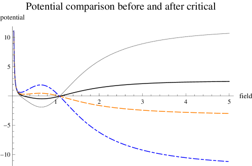
Figure 1: Effective potentials adding a centrifugal repulsion $0.01/\chi^{2}$ after and before critical point of quantum fluctuation in $(F_{4},V_{4})$ model. Common parameters are $(M_{\rm P},\Lambda,\xi_{2},\xi_{4},g)=(1,0.1,1,1,1)$ in the Planck unit: effective potential before critical turning point of $\sqrt{m_{\chi}^{2}-g\langle\phi^{2}\rangle}=5$ in solid black, of $\sqrt{m_{\chi}^{2}-g\langle\phi^{2}\rangle}=10$ in dotted black, and after critical turning point of $\sqrt{g\langle\phi^{2}\rangle-m_{\chi}^{2}}=5$ in dashed orange, and 10 in dash-dotted blue. All potentials decreases in proportion to a negative coefficient $\times\ln\chi$ at field infinity, but existence of potential minimum depends on the next leading term $\propto 1/\chi^{2}$, with coefficients changing with quantum fluctuation.

One may define an effective potential $V_{\rm eff}$ by rewriting the right-hand side of equation for $\ddot{\chi}$ as $-\partial_{\chi}V_{\rm eff}$, to give

$$V_{\rm eff}^{(E)}(\chi)=\frac{1}{5}\int_{\chi_{*}}^{\chi}d\chi F(\chi)\partial_{\chi}V_{\chi g}^{(E)}(\chi)\,,$$ (24)

where $\chi_{*}$ is a few times the Planck mass $M_{\rm P}$. This potential at late times is illustrated for $(F_{4},V_{4})$ models in Fig(1). They have a feature of having a maximum beyond which the derived force pushes the field towards the infinity. The Einstein equation is given, using this effective potential, by

$$(\frac{\dot{a}}{a})^{2}=\frac{1}{6M_{\rm P}^{2}}\left(\frac{5}{2F}\dot{\chi}^{2}+\frac{5}{2F}\frac{(\vec{\nabla}\chi)^{2}}{a^{2}}+V_{\rm eff}^{(E)}(\chi)\right)\,,$$ (25)

while the right-hand side of field equation (21) is given by $-\partial_{\chi}V_{\rm eff}^{(E)}(\chi)$

The effective potential is approximately

$$V_{\rm eff}^{(E)}(\chi)\approx\frac{M_{\rm P}^{4}}{5}\left((\frac{\xi_{2}}{\xi_{4}}+\frac{3m_{\chi}^{2}}{2gM_{\rm P}^{2}})(\frac{M_{\rm P}^{2}}{\chi_{*}^{2}}-\frac{M_{\rm P}^{2}}{\chi^{2}})-\frac{g}{\xi_{4}}\ln\frac{\chi}{\chi_{*}}\right)\,,$$

(26)

to the leading and the next leading orders. $\chi_{*}$ is of order $M_{\rm P}$ taken as an effective starting point of inflation. Its precise value is not important. The asymptotic form of field equation in $(F_{4},V_{4})$ model reduces to

$$\ddot{\chi}+3\frac{\dot{a}}{a}\dot{\chi}-4\frac{\dot{\chi}^{2}}{\chi}=\frac{g}{5\xi_{4}}\frac{M_{\rm P}^{4}}{\chi}\,.$$ (27)

A closed differential equation for the inflaton field after inserting the Hubble rate $\dot{a}/a$ derived from the Einstein equation may be useful for numerical computations, giving the scale factor by a subsequent integration. These equations, (27) and (25), shall be used when we discuss late-time evolution.

III.2 Slow-roll inflation

The de Sitter spacetime characterized by a constant cosmological constant is not eternal in scalar-tensor gravity, and we need to identify the epoch that realizes an approximate de Sitter spacetime. In order to determine this epoch, it is useful to notice a good criterion given by the slow-roll conditions, which place bounds on the slope of potential [13], [7]:

$$|\frac{\partial_{\chi}V_{\rm eff}^{(E)}}{V_{\rm eff}^{(E)}}|\ll\frac{1}{M_{\rm P}}\,,\hskip 14.22636pt|\frac{\partial_{\chi}^{2}V_{\rm eff}^{(E)}}{V_{\rm eff}^{(E)}}|\ll\frac{3}{2M_{\rm P}^{2}}\,.$$ (28)

The potential $V_{\rm eff}^{(E)}$ is nearly a constant and one can take its value $M_{\rm P}^{4}(\xi_{2}/\xi_{4}+3m_{\chi}^{2}/(2gM_{\rm P}^{2}))/5$ in (26). The slow-role conditions above give

$$\chi\gg kM_{\rm P}\;{\rm and}\;\sqrt{\frac{2k}{3}}M_{\rm P}\,,\hskip 8.5359ptk=\frac{\xi_{2}}{\xi_{4}}+\frac{3m_{\chi}^{2}}{2gM_{\rm P}^{2}}\,.$$ (29)

There is no difficulty to impose these conditions.

III.3 Spectral index and tensor-to-scalar ratio

Potential slopes actually give more than this. When inflaton exits horizon and re-enters after inflation, inflaton quantum fluctuations give seeds for the structure formation at late universe. Two important quantities arising from this consideration are the spectral index of density perturbation $n_{s}$ and the ratio of tensor-to-scalar modes $r$. These quantities are given in terms of potential slope parameters [14].

$$n_{s}=1+2M_{\rm P}^{2}\left(2\frac{V_{\rm eff}^{\prime\prime}}{V_{\rm eff}}-3(\frac{V_{\rm eff}^{\prime}}{V_{\rm eff}})^{2}\right)\,,$$ (30)

$$r=16M_{\rm P}^{2}(\frac{V_{\rm eff}^{\prime}}{V_{\rm eff}})^{2}\,.$$ (31)

These simple formulas are valid for single inflaton model defined by a single potential. Our model during inflationary epoch is well approximated by a potential of a single inflaton field, and gives

$$\frac{V_{\rm eff}^{\prime}}{V_{\rm eff}}\approx-\frac{g}{k\xi_{4}}\frac{1}{\xi_{*}}\,,\hskip 8.5359pt\frac{V_{\rm eff}^{\prime\prime}}{V_{\rm eff}}\approx\frac{g}{k\xi_{4}}\left(\frac{1}{\xi_{*}^{2}}-\frac{6k\xi_{4}}{g}\frac{M_{\rm P}^{2}}{\xi_{*}^{4}}\right)\,.$$ (32)

To leading large field approximation, the spectral index and the tensor-to-scalar ratio are related by

$$n_{s}-1+\frac{3}{8}r\approx 4M_{\rm P}^{2}\frac{V_{\rm eff}^{\prime\prime}}{V_{\rm eff}}\,.$$ (33)

Observations have given us $n_{s}\sim 0.965\pm 0.01$ and $r\leq 0.036$ [15], [16]. Our predictions for $n_{s}-1\,,r$ computed using accurate potential and derivative functions are illustrated in Fig(2). Similar plots in other two-parameter planes may also be depicted. There are good chances that observed values are well reproduced in our model if initial $\chi$ values at inflation are within a slow-roll range of $(7\sim 8)M_{\rm P}$.

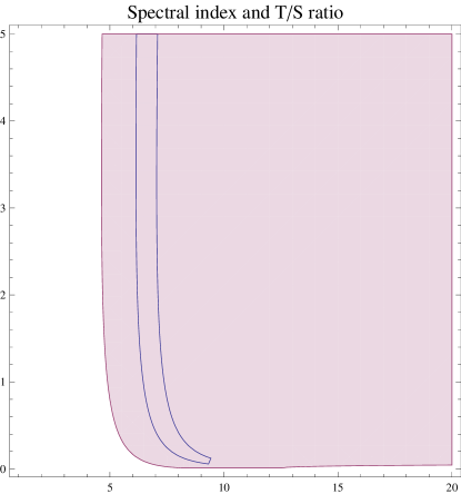
Figure 2: Region of spectral index in the range, $n_{s}-1=0.965\pm 0.01$ (given by a thin region surrounded by two curves) and tensor-to-scalar ratio in $r\leq 0.036$ plotted in $(\chi/M_{\rm P}\,,\xi_{4})$ plane. Other parameters are fixed at $\xi_{2}=1\,,g=2\,,M_{\rm P}=1\,,|m_{\chi}|=7\,,\Lambda=0.1M_{\rm P}^{2}\,,c_{+}=5$.

III.4 Oscillation at the end of inflation

The presence of potential minimum in $V_{\rm eff}^{(E)}(\chi)$ with spontaneously broken Nambu-Goldstone centrifugal force provides a shifted potential minimum away from the origin. The field equation has an approximate form in $(F_{4},V_{4})$ model,

$$\ddot{\chi}+3\frac{\dot{a}}{a}\dot{\chi}-4\frac{\dot{\chi}^{2}}{\chi}=-\partial_{\chi}V_{\rm eff}^{(E)}\,,$$ (34)

$$-\partial_{\chi}V_{\rm eff}^{(E)}\approx M_{\rm P}^{4}\left(\frac{c_{1}}{\chi}-\frac{c_{3}}{\chi^{3}}\right)\,,$$ (35)

$$c_{1}=\frac{g}{5\xi_{4}}\,,\hskip 8.5359ptc_{3}=\frac{3\xi_{4}m_{\chi}^{2}+2g\xi_{2}M_{\rm P}^{2}}{5\xi_{4}^{2}}\,.$$ (36)

The potential form with $m_{\chi}\neq 0$ is qualitatively the same as for the massless $\chi$ field of purely quartic coupling, namely the case of $m_{\chi}=0$. The precise value of parameter $m_{\chi}$ is not important in $c_{3}$.

Oscillation period is characterized by the minimum field point, $\chi_{b}=\chi_{e}$(a constant) and oscillation frequency $\omega$,

$$\chi_{e}=\sqrt{\frac{c_{3}}{c_{1}}}\,,\hskip 14.22636pt\omega^{2}=4M_{\rm P}^{4}\frac{c_{1}^{2}}{c_{3}}\,.$$ (37)

During this phase the anti-friction is

$$\frac{\partial_{\chi}F}{F}\dot{\chi}^{2}\sim 4\frac{\dot{\chi}^{2}}{\chi_{e}}\,,$$ (38)

giving the field equation,

$$\ddot{\chi}+3\frac{\dot{a}}{a}\dot{\chi}-4\frac{\dot{\chi}^{2}}{\chi_{e}}\approx-\omega^{2}(\chi-\chi_{e})\,.$$ (39)

If the potential curvature $\omega^{2}$ is large enough, one can neglect the anti-friction $\propto-\dot{\chi}^{2}/\chi_{e}$.

IV Particle production and symmetry restoration

Inflationary epoch ends with Higgs boson production followed by thermalizing interaction among Higgs boson and other standard model particles, as outlined in [17], [18]. We discuss in the present section another problem related to the second inflaton.

IV.1 Particle production and quantum fluctuation due to inflaton oscillation

We shall discuss $\phi$ quantum production, which occurs for a larger $\chi$ mass than a $\phi$ mass. The quantum $\phi$ system consists of harmonic oscillator aggregates of its frequencies periodically oscillating synchronous to the $\chi$ field oscillation around the potential minimum at $m_{\chi}/\sqrt{g}$. The field equation is linear in $\phi$ field and its Fourier $\vec{q}$ modes $\phi_{q}$ satisfy

$$\ddot{\phi_{q}}+3\frac{\dot{a}}{a}\dot{\phi_{q}}+\frac{q^{2}}{a^{2}}\phi_{q}=-\frac{1}{5}\frac{m_{\phi}^{2}+2g\chi_{e}\chi(t)}{F}\phi_{q}\,.$$ (40)

A large-amplitude oscillating $\chi(t)$ leads to parametric amplification generally characterized as a Floquet-system, which produces $\phi$ quanta, as described in [17], [18].

Particle production is necessarily accompanied by quantum fluctuation due to fluctuation-dissipation theorem. In [18] a formalism is developed to relate quantum fluctuation to dissipation, namely particle production. Their relation is given by

$$\frac{\omega_{q}}{2}\langle\phi_{q}^{2}\rangle=\langle N_{q}\rangle\frac{d^{3}q}{(2\pi)^{3}}\,.$$ (41)

Thus, the zero-point fluctuation $\langle\phi_{q}^{2}\rangle$ of fields is directly related to the produced number of particles $\langle N_{q}\rangle$.

A precise condition for symmetry restoration is formulated by calculating quantum zero-point fluctuation in terms of effective time-dependent $\chi$ mass $M_{\chi}$,

$$\langle\phi^{2}\rangle=\frac{2}{\pi^{2}}\int_{m_{\phi}}^{M_{\chi}/2}d\omega_{q}\sqrt{\omega_{q}^{2}-m_{\phi}^{2}}\sim\frac{M_{\chi}^{2}}{4\pi^{2}}\,,$$ (42)

$$M_{\chi}^{2}=-\partial_{\chi}^{2}V_{\rm eff}\approx\frac{g}{5\xi_{4}}\frac{M_{\rm P}^{4}}{\chi_{b}^{2}}\,.$$ (43)

The condition $M_{\chi}^{2}\geq 0$ is imposed. In this formula we assumed the massless $\phi$ for simplicity. The condition of symmetry restoration is

$$g\langle\phi^{2}\rangle-m_{\chi}^{2}\geq 0\,,\;{\rm or}\;\frac{g}{4\pi^{2}}M_{\chi}^{2}-m_{\chi}^{2}\geq 0\,.$$ (44)

In Fig(3) we illustrate field region in which the symmetry is restored. The symmetry is restored to give quantum fluctuation only when large amplitude $\chi$ oscillation is at work, namely during copious production of $\phi$. If accumulated amount of quantum fluctuation exceeds the negative mass square originally set up, inflaton starts to roll to the field infinity.

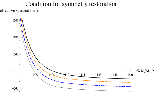
Figure 3: Left-hand side of eq.(44) for a few choices of parameters: common parameters are $\xi_{2}=1,\xi_{4}=1,\Lambda=0.1,g=5,M_{\rm P}=1,c_{+}=5$, and $|m_{\chi}|=$ 5 in solid black, 6 in dashed orange, 7 in dash-dotted blue, and 8 in dotted black. The small field region of positive values gives symmetry restoration.

Let us work out the critical point of quantum fluctuation for symmetry restoration. The next leading term, the term $c_{3}/(2\chi^{2})$, to the leading potential term of $-c_{1}\ln\chi$ at the field infinity (see equations in (36), is shifted as $c_{3}\rightarrow\bar{c}_{3}$;

$$\bar{c}_{3}\sim\frac{1}{5\xi_{4}^{2}}\left(2g\xi_{2}M_{\rm P}^{2}+3\xi_{4}(m_{\chi}^{2}-g\langle\phi^{2}\rangle)\right)\,.$$ (45)

Hence the field can roll down to infinity when quantum fluctuation grows beyond $\langle\phi^{2}\rangle_{\rm cr}$ given by $\bar{c}_{3}=0$:

$$\langle\phi^{2}\rangle_{\rm cr}=\frac{m_{\chi}^{2}}{g}+\frac{2\xi_{2}M_{\rm P}^{2}}{3\xi_{4}}\,.$$ (46)

We may call this critical fluctuation. We illustrate solutions of exact solutions prior to critical fluctuation in Fig(4).

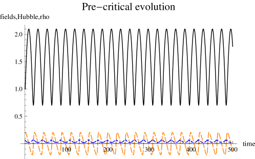
Figure 4: Solution of exact coupled field and Einstein equation taking an effective $\chi$ mass of SSB prior to critical fluctuation: assumed parameters are $\sqrt{m_{\chi}^{2}-g\langle\phi^{2}\rangle}=1/5,g=1,\xi_{2}=5,\xi_{4}=1,\Lambda=0.1$ in the Planck unit $M_{\rm P}=1$. Centrifugal repulsive term in the potential $0.1/\chi^{2}$ is added. $\chi$ field in black, its derivative in dashed orange, Hubble rate in dash-dotted blue, and effective $\Lambda$ in dotted black.

As discussed in more detail below, the inflaton mass $M_{\chi}\propto 1/\chi$ defined in (43) varies with time, ultimately decreasing with redshifts as $\propto(z+1)^{2}$. With decreasing $M_{\chi}$, the equilibrium potential minimum is then recovered again at $m_{\chi}/\sqrt{g}$, violating the condition of symmetry restoration given by (44). This does not pose any problem to the scenario of vanishing cosmological constant just presented, because once the inflaton field passes over a local potential barrier right to $m_{\chi}/\sqrt{g}$, the potential monotonically decreases behaving like $-\ln\chi$ towards the field infinity. What matters is a temporary change of potential shape around the electroweak phase transition, and a later shape change in this region is irrelevant to the cosmological constant problem.

IV.2 Radiation dominated epoch

Time evolution in the radiation-dominated universe of thermalized particles after inflation is described by inflaton field equation,

$$\ddot{\chi}+\frac{3}{2t}\dot{\chi}=\frac{g}{5\xi_{4}}\frac{M_{\rm P}^{4}}{\chi}\,,$$ (47)

where the Hubble rate $H=\dot{a}/a=1/2t$, since the inflaton contribution is negligible at this epoch. Solutions are searched for by assuming an ansatz, $\chi(t)=At(\ln t)^{p}$, and one arrives at approximate solutions,

$$\chi(t)=\sqrt{\frac{2g}{15\xi_{4}}}M_{\rm P}^{2}t\,.$$ (48)

Namely, the first term $\ddot{\chi}$ is negligible compared to the second of right-hand side of eq.(47). Since the redshift factor is defined by $z+1=a(t_{0})/a(t)$ with $t_{0}$ the present cosmic time, this gives a simple relation,

$$\frac{\chi(t)}{\chi(t_{0})}=\frac{t}{t_{0}}=(z+1)^{-2}\,,$$ (49)

$$\chi(t_{0})\approx\sqrt{\frac{1}{30}}\sqrt{\frac{g}{\xi_{4}}}\frac{M_{\rm P}^{2}}{H_{0}}\sim 0.31\times 10^{60}\sqrt{\frac{g}{\xi_{4}}}M_{\rm P}\,,$$ (50)

extrapolating, to the present epoch, the formula $H=1/(2t)$ valid in the radiation dominated epoch, $t_{0}\approx 1/(2H_{0})$. This crude approximation is sufficient for our purpose.

We summarize the potential of entire scalar system consisting of O(4) symmetric real inflaton fields having no quantum number of the electroweak theory and Higgs doublet. In the rolling phase towards the field infinity the Einstein frame potential of these fields is given by

$$V_{\chi H}=-c_{1}M_{\rm P}^{4}\ln\frac{\chi}{M_{\rm P}}+\frac{\lambda_{H}}{4}\,F^{-2}(|H|^{2}-v^{2})^{2}\,.$$ (51)

In the $\chi\rightarrow\infty$ limit the first term in the right-hand side dominates over all other terms.

The $F-$factor is a quartic function of $\chi$, and at the field infinity the factor here is approximately

$$F^{-2}\approx(\xi_{4}(\frac{\chi}{M_{\rm P}})^{4})^{-2}\propto(z+1)^{16}\,.$$ (52)

This contribution at earlier epochs is lots larger than at present. The Higgs boson mass given by (17) thus follows the rule, $\propto F^{-1}\propto(z+1)^{8}$ in radiation-dominated universe.

V Late time acceleration

V.1 Differential equations and its solutions

Basic equations have been already derived in (27) and (25) with the effective potential (26). To recapitulate, the equations for spatially homogeneous mode read as

$$\ddot{\chi}+3\frac{\dot{a}}{a}\dot{\chi}-4\frac{\dot{\chi}^{2}}{\chi}=c_{0}\frac{M_{\rm P}^{4}}{\chi}\,,\hskip 8.5359ptc_{0}=\frac{g}{5\xi_{4}}>0\,,$$ (53)

$$(\frac{\dot{a}}{a})^{2}=\frac{\rho_{\rm DE}}{6M_{\rm P}^{2}}\,,\hskip 8.5359pt\rho_{\rm DE}\approx\frac{M_{\rm P}^{6}}{5\chi_{*}^{2}}(\frac{\xi_{2}}{\xi_{4}}+\frac{3m_{\chi}^{2}}{2gM_{\rm P}^{2}})\,.$$ (54)

We took the leading term for $\rho_{\rm DE}$ in the right-hand side of Einstein equation. The next sub-leading terms shall be discussed shortly.

There is an important relation that holds irrespective of detailed inflaton evolutionary behavior: the Einstein equation immediately tells that the universe is accelerating, and the present value of dark energy density is given by

$$\rho_{\rm DE}(t_{0})=6H_{0}^{2}M_{\rm P}^{2}\sim(2.1\,{\rm meV})^{4}\,.$$ (55)

In the accelerating late-time universe the inflaton field equation reads as

$$\ddot{\chi}+3H_{0}\dot{\chi}-4\frac{\dot{\chi}^{2}}{\chi}=c_{0}\frac{M_{\rm P}^{4}}{\chi}\,,$$ (56)

with a constant Hubble rate $\dot{a}/a\sim H_{0}$. One can readily understand the behavior of time evolution by guessing solutions for the field and verifying its consistency. The ansatz of solution is a power law, $\chi=At^{\alpha}$: the choice of $\alpha=1/2$ gives a balance of the Hubble and the potential terms, to give

$$\chi\approx\sqrt{\frac{2c_{0}}{3H_{0}}}M_{\rm P}^{2}t^{1/2}\,.$$ (57)

Neglected terms are found to be of order $t^{-3/2}$, smaller than the retained term of order $t^{-1/2}$. The validity of potential dominance is illustrated in Fig(5).

A more accurate closed form of inflaton field equation is

$$\ddot{\chi}+\frac{3}{\sqrt{6}M_{\rm P}}\sqrt{\rho_{\rm DE}+\delta\rho}\,\dot{\chi}-4\frac{\dot{\chi}^{2}}{\chi}=c_{0}\frac{M_{\rm P}^{4}}{\chi}\,,$$ (58)

$$\delta\rho=\frac{M_{\rm P}^{4}}{\xi_{4}}\left(\frac{5}{2}\frac{\dot{\chi}^{2}}{\chi^{4}}-\frac{g}{5}\ln\frac{\chi}{\chi_{*}}\right)\,.$$ (59)

It is difficult to numerically solve this equation, but one can conjecture that the solution approaches (57).

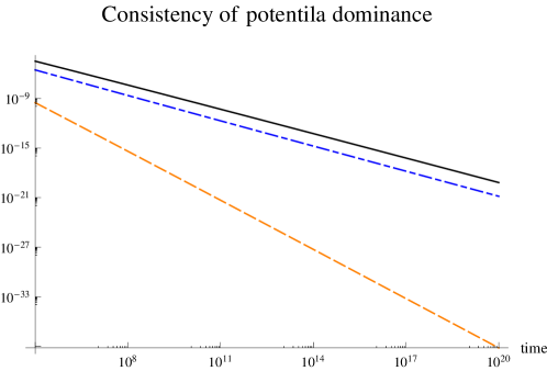
Figure 5: Potential dominance solution is used to compare three terms in the field equation: the force term derived from the potential in solid black, the Hubble term in dashed orange, and the friction term $\propto-\dot{\chi}^{2}/\chi$ in dash-dotted blue. Minor parameter dependences are ignored, taking $c_{0}=1,M_{\rm P}=1$.

V.2 Equation-of-state factor

It may be useful to define the equation-of-state factor $w_{\chi}$ for the inflaton field,

$$w_{\chi}^{(E)}=\frac{\frac{5}{2F}(\dot{\chi}^{2}-\frac{(\vec{\nabla}\chi)^{2}}{3a^{2}})-V_{\rm eff}^{(E)}(\chi)}{\frac{5}{2F}(\dot{\chi}^{2}+\frac{(\vec{\nabla}\chi)^{2}}{a^{2}})+V_{\rm eff}^{(E)}(\chi)}\,.$$ (60)

The energy conservation law for inflaton in conformal gravity is

$$\dot{\rho_{\chi}}=-(3\frac{\dot{a}}{a}+4\frac{\dot{\chi}}{\chi})\frac{5}{F}\rho_{\chi}(1+w_{\chi}^{(E)})\,,$$ (61)

replacing $\dot{\rho_{\chi}}=-3\frac{\dot{a}}{a}\rho(1+w_{\chi})$ in general relativity (GR). This equation was derived by using the field contribution to the energy-momentum tensor in the Einstein frame,

$$T^{(\chi)}_{\mu\nu}=\frac{5}{F}(\partial_{\mu}\chi\partial_{\nu}\chi-\frac{1}{2}g_{\mu\nu}\partial_{\alpha}\chi\partial^{\alpha}\chi)+\frac{1}{F^{2}}V(\chi)g_{\mu\nu}\,.$$ (62)

In GR there is a cancellation between a part of kinetic term $\dot{\chi}^{2}/2$ and potential $V$, to give the pressure $p=w\rho=\frac{(\vec{\nabla}\chi)^{2}}{6a^{2}}$. This cancellation does not work in conformal gravity due to the presence of $F-$factors. It would be instructive to calculate the energy density and the pressure for inflaton field in conformal gravity.

The potential was calculated at field infinity and is given in (26). Three terms in the energy density are given by

$$\rho_{\chi}=\frac{5}{2\xi_{4}}\frac{M_{\rm P}^{4}}{\chi^{4}}(\dot{\chi}^{2}+\frac{(\vec{\nabla}\chi)^{2}}{a^{2}})$$

$$+\frac{M_{\rm P}^{4}}{5}\left((\frac{\xi_{2}}{\xi_{4}}+\frac{3m_{\chi}^{2}}{2gM_{\rm P}^{2}})\frac{M_{\rm P}^{2}}{\chi_{*}^{2}}-\frac{g}{\xi_{4}}\ln\frac{\chi}{\chi_{*}}\right)\,.$$ (63)

With the redshift dependences $\chi\approx 10^{60}\,M_{\rm P}(z+1)^{-2}$, of (49) and (50), and $\xi_{*}=O(M_{\rm P})$, the energy density is dominated by the potential term, and the pressure term given by the second term is completely negligible at moderate redshifts. We thus arrive at the conclusion of effective $w$ factor being $-$1.

Observational data of cosmology is analyzed using $\Omega_{i}=\rho_{i}8\pi G_{N}/(3H^{2})$ for each component $i$, dark energy, cold dark matter, baryon, and radiation, that contributes to the energy density and $w-$factor: $-1,0,0,1/3$, respectively. In our model the energy and the mass density contain the unit factor $F^{-1/2}$ for dark energy and dark matter, and $F^{-\epsilon}$ for baryon and radiation as explained in the next section. There is no problem to interpret data in terms of $\Lambda$ CDM model provided a promising candidate of cold dark matter is identified. The only subtle problem that may arise is derivation of the cosmological bound of neutrino mass, which should be analyzed with great care.

VI Inhomogeneous inflaton modes and candidate cold dark matter

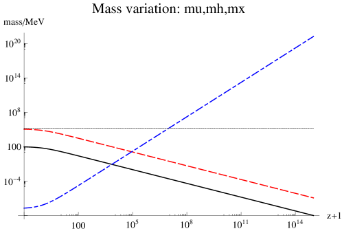
Figure 6: Mass variation: muon mass in solid black, Higgs boson mass in dashed orange, and $\chi$ inflaton mass in dash-dotted blue, plotted against the redshift factor $z+1$, assuming $\epsilon=-0.1$. For a reference the line $v=250GeV/\sqrt{2}$ is shown in dotted black. This variation includes the scale change by $1/F$, hence physically relevant is inflaton mass variation relative to masses of standard model particles.

VI.1 Inhomogeneous inflaton modes

The field equation for spatially inhomogeneous modes of inflaton can be derived by Fourier-decomposing linearized general partial differential equation. This becomes possible by exploiting the space translational invariance under the background field $\chi_{b}(t)$. The linearized equation in terms of deviation $\delta\chi_{q}=\chi-\chi_{b}(t)\propto e^{i\vec{q}\cdot\vec{x}}$ is given by

$$\ddot{\delta{\chi}_{q}}+3\frac{\dot{a}}{a}\dot{\delta{\chi}_{q}}+\frac{q^{2}}{a^{2}}\delta{\chi}_{q}=-M_{\chi}^{2}(z)\delta{\chi}_{q}\,,$$ (64)

$$M_{\chi}(z)=\left(\partial^{2}_{\chi}V_{\rm eff}^{(E)}\right)_{\chi=\chi_{b}}=M_{\chi}(0)(z+1)^{2}\,,$$ (65)

$$M_{\chi}(0)=\sqrt{6}H_{0}\sim 2\times 10^{-33}{\rm eV}\,,$$ (66)

in the radiation-dominated era.

Using $z+1=\sqrt{t_{0}/t}$ valid in the radiation-dominated era, one can analytically solve (64) in terms of cylindrical functions $Z_{\nu}(w)$:

$$\delta\chi_{q}={\cal A}_{q}w^{-1/4}Z_{\nu}(w)\,,$$ (67)

$$w=2q\sqrt{t_{0}t}\,,\hskip 8.5359pt\nu=\frac{\sqrt{1-16(M_{\chi}(0)t_{0})^{2}}}{2}\,.$$ (68)

The value $4M_{\chi}(0)t_{0}=4\sqrt{6}H_{0}t_{0}\sim 100$ gives a purely imaginary $\nu$, the order of cylindrical function. The solution in the $t\rightarrow 0^{+}$ limit is $O(t^{-1/8})\times$ sinusoidally oscillating function of argument $\Im\nu\ln t/2$.

At large times inflaton amplitudes approach the behavior of damped oscillation,

$$\delta\chi_{q}(w=2q\sqrt{t_{0}t})\approx{\cal A}_{q}\sqrt{\frac{2}{\pi}}w^{-3/4}\cos\left(w-\frac{2\nu+1}{4}\pi\right)\,,$$

(69)

for $Z_{\nu}=J_{\nu}$, the Bessel function. A time average of the squared field amplitude over a time span $T>\pi/(q^{2}t_{0})$ is

$$\overline{\delta\chi_{q}^{2}}\approx\frac{{\cal A}_{q}^{2}}{4\pi}(2q\sqrt{t_{0}t})^{-3/2}e^{\pi\Im\nu}\propto t^{-3/4}\,.$$ (70)

This slow decrease behavior differs from the naive expectation $\propto 1/a^{3}\propto t^{-3/2}$ for ordinary cold dark matter in radiation-dominated era. See below on more of this.

In Appendix, we argue that inhomogeneous modes are thermally produced from ambient particles. The amplitude ${\cal A}_{q}$ can then be determined by taking thermal distribution,

$${\cal A}_{q}=\frac{\delta\chi_{q}(z_{EW})}{e^{\sqrt{M_{\chi}^{2}+q^{2}/a^{2}(t_{EW})}/T_{EW}}-1}\,,$$ (71)

when inflatons are produced at the electroweak epoch $t=t_{EM}$. $\delta\chi_{q}(z_{EW})$ is of order $T_{EW}$. One can use the small time limit formula of Bessel function traced back from late times

$$\delta\chi_{q}\approx 2^{-\nu}{\cal A}_{q}w^{\nu-1/4}\,.$$ (72)

After their production, decay of inhomogeneous modes is frozen, and shortly after the electroweak epoch they decouple from the rest of thermal medium. The epoch when they become non-relativistic is estimated by equating the average momentum to the mass ($\sim 2$ meV at the electroweak epoch), which gives the redshift factor,

$$z_{NR}+1=\frac{\pi^{4}}{30\zeta(3)\sqrt{6}}\frac{T_{EW}}{H_{0}(z_{EW}+1)^{2}}\approx 1\times 10^{14}\,.$$ (73)

Thus, it is likely that inhomogeneous inflaton modes become cold dark matter (CDM) shortly after the electroweak phase transition.

VI.2 Time variation of CDM energy density

The formula of inhomogeneous mode energy density is written in terms of field and field derivative;

$$\rho_{\rm CDM}=M_{\rm P}^{4}\left(\frac{5}{2\xi_{4}}\frac{(\dot{\delta\chi})^{2}}{\chi_{b}^{4}}+\frac{5}{2\xi_{4}}\frac{(\vec{\nabla}\delta\chi)^{2}}{a^{2}\chi_{b}^{4}}+\frac{g}{10\xi_{4}}\frac{(\delta\chi)^{2}}{\chi_{b}^{2}}\right)\,.$$

(74)

Redshift dependences of the three terms in the right-hand side are $(z+1)^{13.5}\,,(z+1)^{11.5}\,,(z+1)^{5.5}$, respectively. At latest epochs the last potential term is dominant. We can estimate CDM energy density after the epoch of the radiation-matter equality:

$$\rho_{\rm CDM}(z)\approx\rho_{\rm CDM}(0)(z+1)^{5.5}\,,$$ (75)

$$\rho_{\rm CDM}(0)=\frac{g}{10\xi_{4}}M_{\rm P}^{4}\frac{(\delta\chi_{0})^{2}}{\chi_{0}^{2}}\,,$$ (76)

$$M_{\rm P}^{4}\frac{(\delta\chi_{0})^{2}}{\chi_{0}^{2}}\approx\frac{\pi^{2}T_{EW}^{4}}{15}(z_{EW}+1)^{-3/2}\sim 2\times 10^{21}{\rm eV}^{4}\,,$$

(77)

$$\rho_{\rm CDM}(0)\approx(0.8\,{\rm meV})^{4}\,.$$ (78)

The estimated present CDM energy density $\rho_{\rm CDM}(0)$ falls in an interesting range, and is consistent with the observed dark matter energy density.

A possible problem against identifying inhomogeneous modes as cold dark matter might be in the decrease rate of the energy density, $(z+1)^{5.5/2}$, or $a^{-11/4}$ in terms of scale factor of radiation dominance. This is slightly slower than the usual CDM $a^{-3}$ behavior. This does not seem to be a real problem in analysis of observational data in terms of $\Lambda$ CDM model.

There is another candidate of cold dark matter in our model. It is $\phi-$inflaton. This field satisfies a non-linear equation of the form,

$$\ddot{\phi}+3\frac{\dot{a}}{a}\dot{\phi}-\frac{\partial_{\chi}F}{F}\dot{\phi}-\frac{\vec{\nabla}^{2}\phi}{a^{2}}=\frac{c_{-}^{2}}{a^{6}\phi^{3}}-m_{\phi}^{2}\phi\,.$$ (79)

The potential minimum $\phi_{*}$ is determined by balancing the centrifugal repulsion and the ordinary quadratic mass term in the right-hand side. Around this minimum given by

$$\phi_{*}=a^{-3/2}\sqrt{\frac{c_{-}}{\xi_{4}m_{\phi}(z)}}(\frac{M_{\rm P}}{\chi_{b}})^{2}\,,$$ (80)

$$m_{\phi}(z)=m_{\phi}(0)(z+1)^{2}\,,$$ (81)

$$m_{\phi}(0)\sim\sqrt{30g}H_{0}\sim 5\times 10^{-33}{\rm eV}\,,$$ (82)

one can analyze dumped oscillation in terms of linearized deviation $\delta\phi=\phi-\phi_{*}$. The Fourier mode decomposition $\delta\phi=\sum_{\vec{q}}\delta\phi_{q}e^{i\vec{q}\cdot\vec{x}}$ gives

$$\ddot{\delta\phi_{q}}+(3\frac{\dot{a}}{a}-4\frac{\dot{\chi_{b}}}{\chi_{b}})\dot{\delta\phi_{q}}+\frac{q^{2}}{a^{2}}\delta\phi_{q}=-4m_{\phi}^{2}\delta\phi_{q}\,.$$ (83)

The $\phi-$field equation is essentially similar to the $\chi-$inflaton inhomogeneous mode equation, and $\phi$ quanta are thermally produced in similar fashions to $\chi$ CDM.

Presumably, a more attractive candidate is gravitationally collapsed clumps made of inhomogeneous modes; primordial black holes. As discussed in [19] and briefly mentioned in Appendix, gravity effects measured by $G_{N}M_{\rm clump}^{2}\propto(z+1)^{8}$ grows towards early epochs of our universe if the clump mass $M_{\rm clump}$ is dominated by inhomogeneous inflaton modes. Primordial black holes of mass $\sim 10^{23}$ gr within the horizon at the end of inflation may be copiously produced. They do not over-close the universe due to the present upper bound of energy density $\approx(0.8{\rm meV})^{4}$ of (78).

VII Summary

It is striking that a class of conformal scalar-tensor gravity theories have a rich variety of physics in the early universe, and has a potential of solving the long-standing problem of fine-tuned cosmological constant along with a slow-roll inflation, late-time accelerating universe and cold dark matter. We shall summarize what we have achieved in our model.

In our class of models there are, in addition to standard model lagrangian functionals, two polynomial functions, for which we took quartic polynomials for a simplest successful model. They are conformal and potential functions, and these are functions of four real fields both having O(4) symmetry. The conformal function $F(\chi)$ is positive definite and is a function of inflaton field $\chi$, coupled to the Ricci scalar of metric field in the lagrangian density. The potential function has a O(4) symmetric wine bottle shape and has a minimum away from the field zero origin. A bare cosmological constant may be present in the Jordan metric frame, but in the Einstein frame it is multiplied by $F^{-2}(\chi)$, which may be regarded as an effective cosmological constant variable.

Suppose that the universe started with an inflaton field value larger than $O(5M_{\rm P})$. The effective potential derived by integrating the force term in the inflaton field equation is found to decrease towards a smaller O(4) symmetry breaking point. The slow-roll inflation producing a right amount of the spectral index and satisfying a constraint of the tensor-to-scalar mode ratio consistent with observations is realized by choosing parameters within a wide range.

Towards the end of inflation the inflaton field oscillates around the potential minimum. Two things happen during this oscillation phase; firstly, copious particle production including standard model Higgs boson, and secondly growing accumulated quantum fluctuation. These two are related by the fluctuation-dissipation theorem. Copiously produced particles quickly thermalize among their own interactions, giving a hot big-bang universe. Accumulated quantum fluctuation ultimately restores O(4) symmetry, with inflaton field being pushed back towards the field infinity under a negative logarithmic potential slope. Inflaton field rolls ultimately to the infinity, roughly proportional to the elapsed time, while the energy density stored in inflaton decreases much more slowly, behaving effectively as a constant.

Inhomogeneous mode of inflaton field is shown to have a quantum mass around the Hubble constant $\sim 10^{-33}$eV at present, and they act as a cold dark matter, becoming temporarily dominant after radiation dominance. Finally, the inflaton field takes over and late time accelerating universe begins and lasts till the present, leaving the dark energy density of order, (a few meV)⁴.

Another attractive candidate of the dark matter is primordial black hole due to stronger gravity effects in the early universe.

Baryo-genesis or lepto-genesis can be accommodated in a number of ways, with additional physics input beyond the standard model.

Clearly, many details have to be worked out, but it would be exciting to be able to discuss the entire history of early universe without worrying about the fine-tuning of cosmological constant.

VIII Appendix: Production rate and decay freeze-out of inhomogeneous inflaton modes

In order to discuss production and a possibility of inflaton decay, it is necessary to precisely understand the mass relation of standard model particles, Higgs boson, fermions (quarks and leptons), and the inflaton. A candidate of inflaton cold dark matter (CDM) is identified as the spatially inhomogeneous mode of inflaton field $\chi$, and its time evolution is fully discussed in the text. We mention here that the inflaton mass $M_{\chi}$ is defined by the square root of potential derivative, $\partial_{\chi}^{2}V_{\rm eff}$ in (43), and that it dynamically changes with the cosmic expansion, being proportional to the square redshift, $(z+1)^{2}$. This time dependence is different from those of standard model particles. According to the Weyl scaling to the Einstein metric frame, fermion masses and other boson (Higgs scalar and gauge vector bosons) masses have different redshift differences, $(z+1)^{16}$ and $(z+1)^{8}$, respectively.

But this weird time dependence can be modified and a new rule may be set up such that all standard model particle masses are changed according to the same rule, $(z+1)^{8\epsilon}$. The derivation of modification shall be given separately in a companion paper [19]. We adopt this modification, since it may drastically change time evolution of cold dark matter. At the Feynman rule level, the factor,

$$F^{-2\epsilon}(\chi_{b})\approx\left(\xi_{4}(\frac{\chi_{0}}{M_{\rm P}})^{4}\right)^{-2\epsilon}(z+1)^{16\epsilon}\,,$$ (84)

is attached to all interaction vertexes. With the anticipated numerical estimate of $\chi_{0}(z+1)^{-2}/M_{\rm P}\approx 10^{30}$, the $\epsilon$ factor must be negative to avoid a large suppression. If the inflaton mass is in the denominator of probability amplitude, a further factor $\propto(z+1)^{2}$ is present.

We illustrate mass relations assuming a small negative $\epsilon$ value in Fig(6). From this illustration we arrive at a conclusion that significant inflaton production occurs via high energy collision of fermions such as lepton scattering, $l_{1}+l_{2}\rightarrow l_{3}+l_{4}+\chi$ that arises from Higgs $H_{0}$ exchange in the t-channel emitting $\chi$ by $\chi H_{0}H_{0}$ vertex in the middle. The probability amplitude of this process is product of external wave functions $\bar{\psi}_{3}\psi_{1}\,\bar{\psi}_{4}\psi_{2}\,\varphi_{\chi}$ times

$$\frac{-i\,y_{l}^{2}c_{H}F^{-6\epsilon}(\chi_{b})}{\left((p_{1}-p_{3})-m_{H}^{2}\right)\left((p_{2}-p_{4})-m_{H}^{2}\right)}\,,$$ (85)

where $y_{l}$ is Yukawa coupling constant to lepton, and $c_{H}$ is given in (19).

We shall be content with an order of magnitudes estimate of production cross section instead of calculating that in detail. From dimensional grounds we expect that the cross section is of order,

$$\sigma_{\chi}=\frac{y_{l}^{4}c_{H}^{2}\,F^{-12\epsilon}(\chi_{b})}{(T^{2}+m_{H}^{2})^{2}}\,,$$ (86)

expecting larger values of the incident energy given by the temperature $T$ and the Higgs boson mass to dominate in the denominator. Production rate $\Gamma_{ll\rightarrow\chi}$ is given by $\sigma_{\chi}n_{l}$ where $n_{l}=3\zeta(3)T^{3}/(2\pi^{2})\sim 0.18\,T^{3}$ is the number density of lepton $l$. The ratio of production rate to the Hubble rate is then estimated as

$$\frac{\Gamma_{ll\rightarrow\chi}}{H}\approx 0.01(\frac{m_{l}}{100{\rm MeV}})^{4}(\xi_{4})^{6\epsilon+3/2}g^{-12\epsilon-3/2}$$

$$\cdot\left(0.31\times 10^{30}(\frac{10^{15}}{z+1})^{2}\right)^{-24\epsilon-2}\frac{(T/m_{H})^{3}}{\left(1+(T/m_{H})^{2}\right)^{2}}\,.$$ (87)

For instance, the prefactor becomes $\sim 0.8\times 10^{10}$ if $\epsilon=-1/10$. Decoupling occurs at a redshift $0.1\times$ the electroweak value for this choice of $\epsilon$. For a larger $-\epsilon$ the decoupling redshift becomes closer to the electroweak value. Thus, a range of parameters $\epsilon\leq-0.1$ gives production rates strong enough for thermalized inflaton CDM.

On the other hand, the main inflaton $\chi\rightarrow H_{0}H_{0}$ decay rate compared to the Hubble rate

$$\frac{8\lambda_{H}^{2}}{\pi}(\frac{v^{2}}{\chi_{0}})^{2}\frac{1}{H_{0}}(\xi_{4}\frac{\chi_{0}}{M_{\rm P}})^{-8\epsilon}(z+1)^{16\epsilon+2}\,,$$ (88)

is too small with the same choice of $\epsilon=-1/10$ as before and around the electroweak scale: the $\chi$ CDM decay is essentially frozen despite that it is kinematically allowed.

- [1] S. Weinberg, Rev. Mod. Phys. 61, 1 (1989), and references therein. There are many other proposals for solving the cosmological constant problem. Only an incomplete partial list after this review is given in [2], [3], [4] [5].
- [2] C. Armendaritz-Picon, V. Mukhanov, and P.J. Steinhardt, Phys.Rev.Lett.85, 4438 (2000). Phys.Rev.D63, 103510(2001); Essentials of k-Essence, arXiv: astro-ph/0006373v1 (2000).
- [3] R. Bousso and J. Polchinski, JHEP 6, 006 (2000); “Quantization of four-form fluxes and dynamical neutralization of the cosmological constant”, arXiv: hep-th/0004134 (2000).
- [4] E. Witten: “The cosmological constant from the viewpoint of string theory”, hep-ph/0002297 (2000).
- [5] A.M. Polyakov, Nucl. Phys. B797, 199 (2008).
- [6] M. Yoshimura, “Bifurcated symmetry breaking in scalar-tensor gravity” arXiv: 2112.02835v2 (2021); Accepted for publication in PRD.
- [7] A standard textbook of modern cosmology is S. Weinberg, Cosmology, Oxford University Press, New York (2008).
- [8] Historically, the conformal coupling to Ricci scalar was introduced by the following references, however without the potential term . P. Jordan, Z. Phys. 157, 112 (1959). C. Brans and H. Dicke, Phys. Rev. 124, 925(1961).
- [9] Th. Kaluza, Sitzungber. Preuss. Akad. Wiss. (1920), 966. O. Klein, Z. Phys. 37 (1926), 895.
- [10] N. Manton, Nucl. Phys. B158 (1979) 141. D.B. Fairlie, Phys. Lett. B82 (1979) 97; J. Phys. G5 (1979) L55. P. Forgacs and N. Manton, Comm. Math. Phys. 72 (1980) 15.
- [11] R.A. Malaneya and G. J. Mathews, Physics Reports 229, 145 (1993); “Probing the early universe: a review of primordial nucleosynthesis beyond the standard big bang”
- [12] C.M. Will, Pramana 63, 731 (2004); The Confrontation between General Relativity and Experiment, arXiv:gr-qc/0103036v1 (2002).
- [13] A. Linde, Phys. Lett. B108, 389 (1982); B114, 431 (1982). A. Albrecht and P. Steinhardt, Phys.Rev.Lett. 48, 1220(1982).
- [14] M. Kamionkowski and E.D. Kovetz, Annual Review of Astronomy and Astrophysics, 54, 227 (2016), arXiv:1510.06042.
- [15] Planck Collaboration 2018 VI, Astron. Astrophys. 641, A6 (2020); arXiv:1807.06209.
- [16] BICEP/Keck Collaboration, P.A.R. Ade et al, Phys. Rev. Lett. 127, 151301 (2021); arXiv:2110.00483 (2021).
- [17] L. Kofman, A. Linde, and A.A. Starobinsky, Phys. Rev. Lett. 73, 3195(1994). Phys. Rev. D 56, 3258(1997).
- [18] M. Yoshimura, Progr. Theor. Phys. 94, 873 (1995). This paper discusses explosive particle production caused by external oscillators like periodic inflaton oscillation, leading to parametric amplification, and was applied to the reheating problem after inflation. The formalism developed there may actually be applied to oscillators of general time dependent frequency such as the present model. H. Fujisaki, K. Kumekawa, M. Yamaguchi, and M. Yoshimura, Phys. Rev. D53, 6805 (1996). M. Yoshimura, hep-ph/9605246.
- [19] M. Yoshimura, “Stronger gravity in the early universe”, to be updated to arXiv as a companion paper with the present work. A resolution is proposed there to modify the mass relation in conformal gravity theories by a consistent formulation based on the first principles of quantum field theory. Resulting consequences show that mass ratios among standard model particles do not evolve with time, while the mass ratio of inflaton to standard model particles necessarily evolve.