Analogous Hawking radiation and quantum entanglement in two-component Bose-Einstein condensates: The gapped excitations

Abstract

The condensates of cold atoms at zero temperature in the tunable binary Bose-Einstein condensate system are studied with the Rabi transition between atomic hyperfine states where the system can be represented by a coupled two-field model of gapless excitations and gapped excitations. We set up the configuration of the supersonic and subsonic regimes with the acoustic horizon between them in the elongated two-component Bose-Einstein condensates, trying to mimic Hawking radiations, in particular due to the gapped excitations. The simplified steplike sound speed change is adopted for the subsonic-supersonic transition so that the model can be analytically treatable. The effective-energy gap term in the dispersion relation of the gapped excitations introduces the threshold frequency $\omega_{\text{min}}$ in the subsonic regime, below which the propagating modes do not exist. Thus, the particle spectrum of the Hawking modes significantly deviates from that of the gapless cases near the threshold frequency due to the modified gray-body factor, which vanishes as the mode frequency is below $\omega_{\text{min}}$. The influence from the gapped excitations to the quantum entanglement of the Hawking mode and its partner of the gapless excitations is also studied according to the Peres-Horodecki-Simon (PHS) criterion. It is found that the presence of the gapped excitations will deteriorate the quantumness of the pair modes of the gapless excitations when the frequency of the pair modes in particular is around $\omega\sim\omega_{\text{min}}$. On top of that, when the coupling constant between the gapless and gapped excitations becomes large enough, the huge particle density of the gapped excitations in the small $\omega$ regime will significantly disentangle the pair modes of the gapless excitations. The detailed time-dependent PHS criterion will be discussed.

I Introduction

The program of the analog models of gravity is an attempt to implement laboratory systems to mimic various phenomena that happen in the interplay between general relativity and quantum field theory such as in black holes and the early Universe. The aim is to devise experiments of real laboratory tests that provide insights in the phenomena and further probe the structure of curved-space quantum field theory. The beginning of analog gravity dates back to the pioneering work of Unruh Unruh (1981), who used the sound waves in a moving fluid as an analogue to light waves in curved spacetime and further showed that supersonic fluid can generate a “dumb hole”, an acoustic analogue of a “black hole”. From there, the existence of analog photonic Hawking radiations due to the presence of the acoustic horizon can be theoretically demonstrated. Since its development, the analog gravity program has received much attention to explore fundamental physics through interdisciplinary research among particle/astrophysicists and condensed matter physicists (for a review see Visser and Weinfurtner (2005)). Despite the early start of theoretic investigations, great progress has also been made recently in experimental analog gravity to advance its technologies for realizing the Hawking effects. One of the most successful systems is the Bose-Einstein condensations (BECs). The work of Muñoz de Nova et al. (2019) is a first experimental observation of Hawking radiation extracted from the correlations of the collective excitations that agree with a thermal spectrum with the temperature estimated from analog surface gravity. Also, the time dependence of the Hawking radiation in an analogue black hole is observed in Kolobov et al. (2021).

Most of the works for BEC analogous black holes consider the Hawking radiations due to the gapless excitations analogous to the massless scalar particles. As the Hawking temperature rises to the order of the mass scale of some massive particles, the production of these massive particles also becomes significant Diatlyk (2021). The aspects of the analogue models of the gapped excitations of the BECs have been explored in Jannes et al. (2011); Coutant et al. (2012); Dudley et al. (2018), where the energy-gap term is either induced from the transverse wave number inversely proportional to the size in the perpendicular direction in elongated quasi-one-dimensional system or added by hand as a toy model. One of the main features for the gapped excitations includes the existence of the minimum frequency $\omega_{\rm min}$, below which in the subsonic regime the propagating modes do not survive resulting in the total reflection of radiation coming from the supersonic regime at the horizon. The other feature is that solving the dispersion relation can find the nonvanishing zero-frequency mode where their density-density correlation functions reveal the undulation phenomenon in the supersonic regime. In this work, we will focus on the gapped excitations created from the binary BECs. Two-component BECs have been experimentally studied using the mixture of atoms with two hyperfine states of ${}^{87}\text{Rb}$ Tojo et al. (2010) or the mixture of two different species of atoms Modugno et al. (2002); Thalhammer et al. (2008); Papp et al. (2008); McCarron et al. (2011); Cipriani and Nitta (2013). In the analogue gravity program, the class of two-component BECs subject to laser- or radio-wave induced Rabi transition between different atomic hyperfine states has been proposed to serve as an “emergent” spacetime model, which provides very rich spacetime geometries, such as a specific class of pseudo-Finsler geometries, and both bimetric pseudo-Riemannian geometries and single-metric pseudo-Riemannian geometries of interest in cosmology and general relativity Fischer and Schützhold (2004); Visser and Weinfurtner (2005); Liberati et al. (2006a, b); Weinfurtner et al. (2007). In fact, this class of the two-component BEC systems with the Rabi interaction exhibits two types of excitations on condensates: the gapless excitations due to the “in phase” oscillations between two respective density waves of the binary system and the gapped excitation stemming from the “out-of-phase” oscillations of the density waves in the presence of the Rabi transition, which are respectively analogous of the Goldstone modes and the Higgs modes in particle physics. In addition, in Syu et al. (2020) the dynamics of collective atomic motion by choosing tunable scattering lengths through Feshbach resonances has been studied with the introduced effective parameter characterizing the miscible or immiscible regime of binary condensates and their stabilities.

In this system, we plan to set up the configuration of the supersonic and subsonic regimes with the acoustic horizon between them. We consider the simplified steplike sound speed profile to implement the subsonic-supersonic transition in the elongated two-component Bose-Einstein condensates using the tunable couplings between the atoms through the Feshbach resonances Hamner et al. (2011, 2013) so that the configuration can be analytically treatable. Although the problem of this sudden transition gives the infinity acoustic surface gravity, the corresponding Hawking temperature still can be read off from the obtained spectrum of the Hawking modes. More realistic transitions can be considered in the waterfall configuration that relies on full numerical studies to explore its physics. The experimentally spatial variation of the interaction strengths to fit into the configuration is challenged but feasible Clark et al. (2015); Arunkumar et al. (2019); Di Carli et al. (2020). We first find the dispersion relation of the gapped excitations and identify the various modes in both supersonic and subsonic regimes. The energy-gap term is governed by the Rabi-coupling constant $\Omega$ between two hyperfine states of Bose-Einstein condensates Visser and Weinfurtner (2005), $m_{\text{eff}}\propto\sqrt{\Omega}$, which is tunable experimentally. In addition, a spatial varying of the Rabi-coupling constant is also doable experimentally Arunkumar et al. (2019), which allows to design two different effective-energy gaps on the subsonic and supersonic regimes. The matching between two sets of the wave functions in sub/supersonic regimes allows to define the $S$-matrix, whose elements can be experimentally determined from the density-density correlation functions Muñoz de Nova et al. (2019). One of the main results in this paper then comes from the study of the quantum entanglement between the Hawking mode and its partner of the gapped excitations by employing the Peres-Horodecki-Simon (PHS) criterion Horodecki et al. (1996); Horodecki (1997); Simon (2000). On top of that, to this binary Bose-Einstein condensate system, it provides the opportunity to study the analogue gravity phenomena in the open quantum system, where the gapless excitations are treated as the system and the gapped excitations as an environment. The same idea has been employed to examine the effect of quantum fluctuations due to the gapped excitations on phonon propagation in the binary BECs system to build up an analogous model of the light cone fluctuations induced by quantum gravitational effects in Syu et al. (2019). Here we study the entanglement between the Hawking mode and its partner of the gapless excitations under the influence of the environment of the gapped excitations.

We organize this paper as follows. In Sec. II, we introduce the model of interest and construct the gapped excitations in the supersonic/subsonic configuration where the acoustic horizon is present between them in a binary BECs system. In Sec. III, the matching of the mode functions of two sides of the acoustic horizon is carried out to obtain the scattering coefficients for three outgoing channels. In Sec. IV, we study density-density correlation functions. Section V is devoted to the study of the nonseparability of the gapless excitations influenced by the gapped excitations. We conclude the work in Sec. VI.

II The model

II.1 The Bogoliubov-de Gennes equations in coupled Bose condensates

We consider the binary BECs of the same atoms in two different internal hyperfine states. We then assume that a strong cigar-shape trap potential is used where the size of the trap $L_{x}$ along the axial direction, say in the $x$-direction is much larger than the size of $L_{r}$ along the radial direction. Therefore, the system (in units of $\hbar=k_{B}=1$) can be treated in the pseudo-one-dimension with the Lagrangian given by

$$L_{\text{1D}}= \int dx\Bigg{\{}\sum_{a=A,B}\left[\frac{i}{2}\left(\hat{\Psi}_{a}^{\dagger}{\partial_{t}\hat{\Psi}_{a}}-\hat{\Psi}_{a}{\partial_{t}\hat{\Psi}_{a}^{\dagger}}\right)-\left(\frac{1}{2m}\partial_{x}\hat{\Psi}_{a}^{\dagger}\partial_{x}\hat{\Psi}_{a}+V_{a}\hat{\Psi}_{a}^{\dagger}\hat{\Psi}_{a}+\frac{U_{aa}}{2}\hat{\Psi}_{a}^{\dagger}\hat{\Psi}_{a}^{\dagger}\hat{\Psi}_{a}\hat{\Psi}_{a}\right)\right]$$

$$\qquad\qquad\qquad-\,U_{AB}\hat{\Psi}_{A}^{\dagger}\hat{\Psi}_{B}^{\dagger}\hat{\Psi}_{A}\hat{\Psi}_{B}+\frac{\Omega}{2}(\hat{\Psi}_{A}\hat{\Psi}_{B}^{\dagger}+\hat{\Psi}_{A}^{\dagger}\hat{\Psi}_{B})\Bigg{\}}\;,$$ (1)

where $m$ is atomic mass and $V_{A},\,V_{B}$ are the external potential along the axial direction on the hyperfine states $A$ and $B$. The field operators obey the equal-time commutation relations

$$[\hat{\Psi}_{a}(x,t),\hat{\Psi}_{b}^{\dagger}(x^{\prime},t)]=\delta_{ab}\delta(x-x^{\prime})\,.$$ (2)

The interaction strengths of atoms between the same hyperfine states and different hyperfine states are given by $U_{AA},\,U_{BB}$ and $U_{AB}$, respectively. The coupling strengths are related with the scattering lengths $a$ as $U=2{a}/mL_{r}^{2}$. Experimentally, the values of scattering lengths can be tuned using Feshbach resonances such as two hyperfine states of ${}^{87}\text{Rb}$ Thalhammer et al. (2008); Tojo et al. (2010). In addition, we introduce a Rabi-coupling term by shining the laser field or applying the radio wave with the strength given by the Rabi frequency $\Omega$.

The corresponding time-dependent equations of motion are obtained as

$$i\partial_{t}\hat{\Psi}_{A}=\left[-\frac{1}{2m}\partial_{x}^{2}+V_{A}(x)+U_{AA}\hat{\Psi}_{A}^{\dagger}\hat{\Psi}_{A}+U_{AB}\hat{\Psi}_{B}^{\dagger}\hat{\Psi}_{B}\right]\hat{\Psi}_{A}-\frac{\Omega}{2}\hat{\Psi}_{B}\,,$$ (3a)

$$i\partial_{t}\hat{\Psi}_{B}=\left[-\frac{1}{2m}\partial_{x}^{2}+V_{B}(x)+U_{BB}\hat{\Psi}_{B}^{\dagger}\hat{\Psi}_{B}+U_{AB}\hat{\Psi}_{A}^{\dagger}\hat{\Psi}_{A}\right]\hat{\Psi}_{B}-\frac{\Omega}{2}\hat{\Psi}_{A}\,.$$ (3b)

The condensate wave functions are given by the expectation value of the field operator $\langle\hat{\Psi}_{a}\rangle=\psi_{a}e^{-i\mu t}$, where they are governed by the stationary Gross-Pitaevskii (GP) equations Pethick and Smith (2008)

$$\mu{\psi}_{A}=\left[-\frac{1}{2m}\partial_{x}^{2}+V_{A}(x)+U_{AA}|{\psi}_{A}|^{2}+U_{AB}|{\psi}_{B}|^{2}\right]{\psi}_{A}-\frac{\Omega}{2}{\psi}_{B}\,,$$ (4a)

$$\mu{\psi}_{B}=\left[-\frac{1}{2m}\partial_{x}^{2}+V_{B}(x)+U_{BB}|{\psi}_{B}|^{2}+U_{AB}|{\psi}_{A}|^{2}\right]{\psi}_{B}-\frac{\Omega}{2}{\psi}_{A}\,,$$ (4b)

with the chemical potential $\mu$. The condensate wave functions define the density $\rho_{a}$ and the phase $\theta_{a}$

$$\psi_{a}(x)=\sqrt{\rho_{a}(x)}e^{i\theta_{a}(x)}.$$ (5)

Meanwhile, the continuity equation gives the relations

$$v_{a}(x)\rho_{a}(x)=\text{constant}$$ (6)

with the condensate-flow velocities $\partial_{x}\theta_{a}(x)/m=v_{a}(x)$.

Here we choose the scattering parameters in this binary systems so as to have a stable and miscible state of the background condensates where $\rho_{A}=\rho_{B}=\rho$ and $\theta_{A}=\theta_{B}=\theta$, and also $U_{AA}=U_{BB}=U$ Hamner et al. (2011, 2013). The detailed analysis of the choice of the parameters can be found in our previous work Syu et al. (2019). We further assume that $\rho=\rho_{0}$ is a constant across the whole condensate. We also consider the constant condensate-flow velocity $v_{A}=v_{B}=-v\,(v>0)$ from the positive $x$ to the negative $x$. For the interaction strengths, we consider the steplike change for $U(x)$, namely

$$U(x)=\left\{\begin{array}[]{ll}U_{l}\,,\qquad x<0,\\ U_{r}\,,\qquad x\geq 0,\\ \end{array}\right.$$ (9)

giving the steplike change of the sound speed across $x=0$ while keeping $U_{AB}$ and $\Omega$ uniform across the condensate. The experimentally spatial variation of the interaction strengths is challenging but feasible Clark et al. (2015); Arunkumar et al. (2019); Di Carli et al. (2020). Additionally, the external potential is chosen to satisfy Carusotto et al. (2008); Recati et al. (2009)

$$V_{l}+(U_{l}+U_{AB})\rho_{0}-\Omega/2=V_{r}+(U_{r}+U_{AB})\rho_{0}-\Omega/2\,.$$ (10)

The perturbations around the stationary wave function are defined through

$$\hat{\Psi}_{a}=\langle\hat{\Psi}_{a}\rangle(1+\hat{\phi}_{a})\,,$$ (11)

where the perturbed fields $\hat{\phi}_{a}$ obey the equal-time commutation relations

$$\left[\hat{\phi}_{a}(x,t),\hat{\phi}^{\dagger}_{b}(x^{\prime},t)\right]=\frac{1}{\rho_{0}}\delta_{ab}\delta(x-x^{\prime})$$ (12)

with $a=A,B$. Substituting (11) into (3) and using the GP equations we found the Bogoliubov-de Gennes equations

$$i\partial_{t}{\hat{\phi}}_{A}= -\frac{1}{2m}\partial_{x}^{2}\hat{\phi}_{A}-\frac{i}{m}\partial_{x}\theta\partial_{x}\hat{\phi}_{A}+U\rho_{0}(\hat{\phi}_{A}+\hat{\phi}_{A}^{\dagger})+U_{AB}\rho_{0}(\hat{\phi}_{B}+\hat{\phi}_{B}^{\dagger})+\frac{\Omega}{2}(\hat{\phi}_{A}-\hat{\phi}_{B}),$$ (13a)

$$i\partial_{t}{\hat{\phi}}_{B}= -\frac{1}{2m}\partial_{x}^{2}\hat{\phi}_{B}-\frac{i}{m}\partial_{x}\theta\partial_{x}\hat{\phi}_{B}+U\rho_{0}(\hat{\phi}_{B}+\hat{\phi}_{B}^{\dagger})+U_{AB}\rho_{0}(\hat{\phi}_{A}+\hat{\phi}_{A}^{\dagger})+\frac{\Omega}{2}(\hat{\phi}_{B}-\hat{\phi}_{A})\,,$$ (13b)

where $U$ has a steplike form across $x=0$.

The system of equations (13) can be further decoupled by means of the field transformation

$$\hat{\phi}_{d}=\frac{1}{\sqrt{2}}(\hat{\phi}_{A}+\hat{\phi}_{B})\,,$$ (14a)

$$\hat{\phi}_{p}=\frac{1}{\sqrt{2}}(\hat{\phi}_{A}-\hat{\phi}_{B})\,,$$ (14b)

where the fields $\hat{\phi}_{d}$ and $\hat{\phi}_{p}$ are due to the density and polarization fluctuations, respectively. It will be seen that the field $\hat{\phi}_{d}$ of the gapless excitations and the field $\hat{\phi}_{p}$ of the gapped excitations are analogous to the Goldstone and Higgs modes in particle physics.

In this time-translational invariant system, the field operators $\hat{\phi}_{d}$ and $\hat{\phi}_{p}$ can be decomposed in the frequency domain

$$\hat{\phi}_{d}(x,t)=\sum_{j}\int d\omega\left[\hat{a}_{\omega j}\phi_{d\,\omega j}(x)e^{-i\omega t}+\hat{a}^{\dagger}_{\omega j}\varphi^{\ast}_{d\,\omega j}(x)e^{i\omega t}\right],$$ (15a)

$$\hat{\phi}_{p}(x,t)=\sum_{j}\int d\omega\left[\hat{b}_{\omega j}\phi_{p\,\omega j}(x)e^{-i\omega t}+\hat{b}^{\dagger}_{\omega j}\varphi^{\ast}_{p\,\omega j}(x)e^{i\omega t}\right]\,.$$ (15b)

Apart from the integration over the various frequencies $\omega$, for each $\omega$, there exist either the outgoing channels or incoming channels $j$ to be summed over that will be discussed later. Notice that in the above decomposition, the propagating modes are involved where the range of the frequency for each channel $j$ of the gapless and gapped excitations for having the propagating modes can be different and relies on the dispersion of relation to be seen next. The detailed expansions will be shown in a precise manner below when all the modes in each side of $x$ are determined. In (15), the creation and annihilation operators satisfy the canonical commutation relations, namely

$$\left[\hat{a}_{\omega j},\hat{a}^{\dagger}_{\omega^{\prime}j^{\prime}}\right]=\left[\hat{b}_{\omega j},\hat{b}^{\dagger}_{\omega^{\prime}j^{\prime}}\right]=\delta_{jj^{\prime}}\delta(\omega-\omega^{\prime}).$$ (16)

Substituting (14) into (13), one obtains the wave equations for the mode functions $\phi_{\omega}(x)$ and $\varphi_{\omega}(x)$

$$\left[\left(\omega-iv\partial_{x}\right)+\frac{1}{2m\rho_{0}}\rho_{0}\partial^{2}_{x}\right]\,{\phi}_{d\,\omega}-\left[\left({U}+{U}_{AB}\right)\rho_{0}\right]\left({\phi}_{d\,\omega}+{\varphi}_{d\,\omega}\right)=0,$$ (17a)

$$\left[\left(\omega-iv\partial_{x}\right)-\frac{1}{2m\rho_{0}}\rho_{0}\partial^{2}_{x}\right]\,{\varphi}_{d\,\omega}+\left[\left({U}+{U}_{AB}\right)\rho_{0}\right]\left({\phi}_{d\,\omega}+{\varphi}_{d\,\omega}\right)=0,$$ (17b)

and

$$\left[\left(\omega-iv\partial_{x}\right)+\frac{1}{2m\rho_{0}}\rho_{0}\partial_{x}^{2}\right]\,{\phi}_{p\,\omega}-\left[\left({U}-{U}_{AB}\right)\rho_{0}+\frac{{\Omega}}{2}\right]\left(\phi_{p\,\omega}+\varphi_{p\,\omega}\right)-\frac{\Omega}{2}\left(\phi_{p,\omega}-\varphi_{p\,\omega}\right)=0,$$ (18a)

$$\left[\left(\omega-iv\partial_{x}\right)-\frac{1}{2m\rho_{0}}\rho_{0}\partial_{x}^{2}\right]\,\varphi_{p\,\omega}+\left[\left({U}-{U}_{AB}\right)\rho_{0}+\frac{{\Omega}}{2}\right]\left(\phi_{p,\omega}+\varphi_{p\,\omega}\right)-\frac{\Omega}{2}\left(\phi_{p,\omega}-\varphi_{p\,\omega}\right)=0\,.$$ (18b)

Together with (12), the normalization of the mode functions is given by

$$\int dx\,[\phi_{s\,\omega j}(x)\phi^{*}_{s\,\omega^{\prime}j^{\prime}}(x)-\varphi^{\ast}_{s\,\omega j}(x)\varphi_{s\,\omega^{\prime}j^{\prime}}(x)]=\frac{\delta_{jj^{\prime}}\delta(\omega-\omega^{\prime})}{\rho_{0}}\,$$ (19)

with $s=d,p$.

II.2 Plane wave solutions and dispersion relations

Assuming the plane wave solutions for each side of $x=0$ in the background of the homogenous condensate given by

$$\phi_{s\,\omega}(x,t)=A_{s\,k}e^{-i\omega t+ikx},$$ (20a)

$$\varphi_{s\,\omega}(x,t)=B_{s\,k}e^{-i\omega t+ikx},$$ (20b)

we obtain the dispersion relation for the gapless excitations

$$(\omega+vk)^{2}=c_{d}^{2}k^{2}+\frac{k^{4}}{4m^{2}}\,$$ (21)

with the sound velocity

$$c_{d}=\sqrt{\frac{\left({U}+{U}_{AB}\right)\rho_{0}}{m}}\,.$$ (22)

Also the dispersion relation for the gapped excitations are found to be

$$(\omega+vk)^{2}=c_{p}^{2}k^{2}+\frac{k^{4}}{4m^{2}}+m_{\text{eff}}^{2}$$ (23)

with the speed of the excitations

$$c_{p}=\sqrt{\frac{\left({U}-{U}_{AB}\right)\rho_{0}+\Omega}{m}}$$ (24)

and the effective-energy gap term

$$m_{\text{eff}}=\sqrt{2\left({U}-{U}_{AB}\right)\rho_{0}\Omega+\Omega^{2}}\,,$$ (25)

due to the Rabi-coupling effects Cominotti et al. (2022). The healing length of two types of the excitations is given respectively by

$$\xi_{s}=\frac{1}{mc_{s}}\;,\;\;\;s=d,p\;.$$ (26)

The steplike change of the parameters in (9) reflects in the sudden change of sound speeds  (22), (24) and effective-energy gap in (25) at $x=0$.

Figure 1: The schematic plot depicts two sides of $x=0$. The supersonic region $x<0$ has the sound speed $c_{l}<v$, while the subsonic region $x>0$ has the sound speed $c_{r}>v$. This setting is achieved by tuning the intraspecies interaction as $U_{r}>U_{l}$ in (9). This works for both gapless and gapped excitations.

The mode amplitudes are obtained from the wave equations (17)-(18). According to the normalization conditions (19), the coefficients of the plane wave solutions in (20) follow the relation

$$|A_{s\,k}|^{2}-|B_{s\,k}|^{2}=\pm\frac{1}{2\pi\rho_{0}}\left|\frac{dk}{d\omega}\right|.$$ (27)

After some algebra we find

$$A_{d\,k}=\frac{\omega+vk+k^{2}/2m}{\sqrt{8\pi\rho_{0}(k^{2}/2m)v_{g}(\omega+vk)}},\qquad B_{d\,k}=\frac{-(\omega+vk)+k^{2}/2m}{\sqrt{8\pi\rho_{0}(k^{2}/2m)v_{g}(\omega+vk)}},$$ (28)

$$A_{p\,k}=\frac{\omega+vk+k^{2}/2m+\Omega}{\sqrt{8\pi\rho_{0}(k^{2}/2m+\Omega)v_{g}(\omega+vk)}},\qquad B_{p\,k}=\frac{-(\omega+vk)+k^{2}/2m+\Omega}{\sqrt{8\pi\rho_{0}(k^{2}/2m+\Omega)v_{g}(\omega+vk)}},$$ (29)

where $v_{g}$ is the group velocity $v_{g}=d\omega/dk$. In (27), the positive(negative) sign corresponds to positive(negative) norm branch.

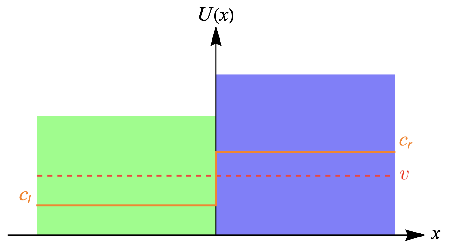
In order to create Hawking radiations, one needs the supersonic and subsonic configuration such that

$$c_{d,l}<v<c_{d,r},$$ (30a)

$$c_{p,l}<v<c_{p,r},$$ (30b)

through the choice of $U_{l}<U_{r}$ in each side of $x=0$ while keeping the flow velocity of the condensates a constant. The schematic plot of the setup is in Fig. 1. The Mach numbers are defined as Larré et al. (2012); Michel et al. (2016)

$$m_{s,l}=\frac{v}{c_{s,l}},\qquad\text{and}\qquad m_{s,r}=\frac{v}{c_{s,r}}\;,\qquad s=d,p\,.$$ (31)

The requirement $m_{s,r}<1<m_{s,l}$ leads to the subsonic region ($x>0$) and the supersonic region ($x<0$) separated by a sudden change of the speed at $x=0$ so that the acoustic horizon emerges. Analogous Hawking radiations given by the gapless excitations have been studied extensively Mayoral et al. (2011). Here we would like to focus on the gapped excitations instead, which themselves can create analogous Hawking radiations. Additionally, turning on the interaction between the gapless and gapped excitations opens the possibility to study how the gapped excitations influence the analogous Hawking radiations from the gapless excitations.

II.3 Gapped excitation modes

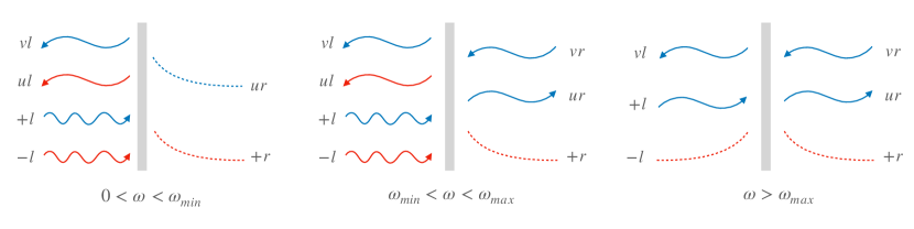
We now investigate the wave numbers of gapped excitations with a fixed frequency $\omega$ from solving the dispersion relation (23). Dispersive effects of the system lead to four solutions for the wave numbers. In the supersonic region or downstream region in $x<0$ with $c_{p,l}<v$, the solutions are qualitatively illustrated in Fig. 2. Two of the solutions $k_{+l},k_{vl}$ are from the dispersion of the relation of the positive comoving frequencies branches and the other two $k_{-l},k_{ul}$ are from the negative comoving frequencies branches when $\omega<\omega_{\text{max}}$. When $\omega>\omega_{\text{max}}$, the solutions of the wave numbers $k_{-l},k_{ul}$ will change to complex values, leaving two real-number solutions $k_{+l},k_{vl}$ only. The wave number $k_{\text{max}}$ and the frequency $\omega_{\text{max}}$ are determined by requiring $\frac{d\omega}{dk}|_{k=k_{\text{max}}}=0$, from the dispersion of relation in the negative comoving frequencies branch, namely

$$\omega=-vk-\sqrt{c_{p,l}^{2}k^{2}+\frac{k^{4}}{4m^{2}}+m_{\text{eff},l}^{2}}\;\;.$$ (32)

Figure 2: The frequency $\omega$ varies with wave number $k$ according to the dispersion relation of gapped excitation (23) (solid line with lighter color) and gapless excitation (21) (dashed line with darker color). In the left panel, a given $\omega$ gives four real-valued roots when $\omega<\omega_{\text{max}}$. However, in the right panel two real-valued roots exist only for $\omega\geq\omega_{\text{min}}$. We consider the single-metric geometry $c_{p}=c_{d}$.

To have analytical expression of $\omega_{\text{max}}$ and $k_{\text{max}}$, we consider small $m_{\text{eff},l}$ limit, where $mc^{2}_{p,l}\approx mv^{2}\gg m_{\text{eff},l}$, leading to $U\rho_{0}\gg\Omega$. Then, to order $m^{2}_{\text{eff},l}$, the solution of $k_{\text{max}}$ can be expressed as $k_{\text{max}}=k_{\text{max}}^{\scriptscriptstyle(0)}+k_{\text{max}}^{\scriptscriptstyle(1)}$, where

$$k_{\text{max}}^{\scriptscriptstyle(0)}=-\frac{m\sqrt{v\sqrt{8c_{p,l}^{2}+v^{2}}-4c_{p,l}^{2}+v^{2}}}{\sqrt{2}},$$ (33)

corresponds to the gapless case Mayoral et al. (2011), and the correction due to $m_{\rm eff}$ is obtained as

$$k^{\scriptscriptstyle(1)}_{\max}=\frac{2m^{2}\left[2c_{p,l}^{2}m^{2}+(k_{\text{max}}^{\scriptscriptstyle(0)})^{2}\right]}{(k_{\text{max}}^{\scriptscriptstyle(0)})^{3}\left[6c_{p,l}^{2}m^{2}+(k_{\text{max}}^{\scriptscriptstyle(0)})^{2}\right]}m_{\text{eff},l}^{2}+\mathcal{O}(m_{\text{eff},l}^{3})\,.$$ (34)

The resulting $\omega_{\text{max}}$ can be then approximated by $\omega_{\text{max}}=\omega_{\text{max}}^{\scriptscriptstyle(0)}+\omega_{\text{max}}^{\scriptscriptstyle(1)}$ with

$$\omega_{\text{max}}^{\scriptscriptstyle(0)}=-vk_{\text{max}}^{\scriptscriptstyle(0)}-\sqrt{c_{p,l}^{2}(k_{\text{max}}^{\scriptscriptstyle(0)})^{2}+\frac{(k_{\text{max}}^{\scriptscriptstyle(0)})^{4}}{4m^{2}}}\,,$$ (35)

$$\omega_{\text{max}}^{\scriptscriptstyle(1)}=\frac{2m^{2}[2c_{p,l}^{2}m^{2}\omega_{\text{max}}^{\scriptscriptstyle(0)}+2(k_{\text{max}}^{\scriptscriptstyle(0)})^{3}v+3(k_{\text{max}}^{\scriptscriptstyle(0)})^{2}\omega_{\text{max}}^{\scriptscriptstyle(0)}]}{(k_{\text{max}}^{\scriptscriptstyle(0)})^{4}[6c_{p,l}^{2}m^{2}+(k_{\text{max}}^{\scriptscriptstyle(0)})^{2}]}m_{\text{eff},l}^{2}+\mathcal{O}(m_{\text{eff},l}^{3})\,.$$ (36)

As long as $c_{p,l}<v$, $\omega_{\text{max}}^{\scriptscriptstyle(1)}$ is negative, leading to a smaller value of $\omega_{\text{max}}$ due to the effective-energy gap term $m_{\text{eff},l}$ as compared with $\omega_{\text{max}}^{\scriptscriptstyle(0)}$ corresponding to the gapless cases. The existence of the two real-number solutions of the wave numbers in the negative comoving frequencies branch allows the quantum states with negative norm that open a window to trigger the subsequent analogous Hawking radiation. Roughly speaking, the above analytical results can provide an estimate of the value of $\omega_{\text{max}}$.

In the subsonic region ($c_{p,r}>v$) and also in the upstream for $x>0$, when $\omega>\omega_{\text{min}}$, there are two solutions $k_{ur},k_{vr}$ of the real numbers obtained from the positive comoving frequencies branch and the other two wave numbers $k_{\pm r}$ of the complex numbers from the negative comoving frequencies branch. See Figs. 2 and 3 for more details.

In fact, from the supersonic to subsonic region, the solution of $k_{u}$ shifts from the negative comoving frequencies branch to the positive comoving frequencies branch whereas the solution $k_{+}$ shifts in stead from the positive comoving frequencies branch to the negative comoving frequencies branch, then becoming complex valued in the subsonic region. On the contrary, the solutions of $k_{v}$ and $k_{-}$ remain in the positive and negative comoving frequencies branches on both regions, but $k_{-}$ becomes complex valued in the subsonic region. The minimum frequency $\omega_{\text{min}}$ can be obtained, when two real wave number solutions merge, with the approximate value in the small $m_{\text{eff}}$ limit, namely $mc^{2}_{p}\approx mv^{2}\gg m_{\text{eff}}$ as Coutant et al. (2012); Balbinot et al. (2019)

$$\omega_{\text{min}}\simeq\sqrt{\frac{c_{p,r}^{2}-v^{2}}{c_{p,r}^{2}}}m_{\text{eff},r}.$$ (37)

For $\omega<\omega_{\text{min}}$, all four wave numbers are complex values, where two of them are the decaying modes and the other two are growing modes. The propagating modes together with the decaying modes will be taken into account on the matching at $x=0$ between two sides of the modes. Here we assume that the growing modes will not be excited. In Fig. 3, we draw the corresponding moving direction of each mode according to the sign of the group velocity $v_{g}$.

Figure 3: Schematic representation of the scattering modes and the decaying modes. In the downstream (supersonic) region, there are four plane wave modes, while in the upstream (subsonic) region, there are only two plane wave modes and one decaying mode. The amplitudes for each mode can be solved by the matching conditions in (49).

The analytical solutions of the wave numbers can only be explored in the limits of small frequency $\omega$ and the effective-energy gap $m_{\text{eff}}$ when $\mu\equiv m_{\text{eff}}/mc_{p}^{2}\ll 1$ and $\nu\equiv\omega/mc_{p}^{2}\ll 1$. In the case of the supersonic wave, for $\omega<\omega_{\text{max}}$, two of the solutions with small wave numbers of order much smaller than $1/\xi_{p}$ in (26) are obtained by treating the term $k^{4}/4m^{2}$ in the dispersion relation (23) perturbatively to yield

$$k_{v}=\frac{v\,\omega+\sqrt{(v^{2}-c_{p}^{2})m_{\text{eff}}^{2}+\omega^{2}c_{p}^{2}}}{c_{p}^{2}-v^{2}}\Bigg{\{}1-\frac{c_{p}^{4}\left[v\,\nu+\sqrt{(v^{2}-c_{p}^{2})\mu^{2}+\nu^{2}c_{p}^{2}}\right]^{3}}{8(c_{p}^{2}-v^{2})^{3}\sqrt{(v^{2}-c_{p}^{2})\mu^{2}+\nu^{2}c_{p}^{2}}}+\mathcal{O}{(\nu^{4},\mu^{4})}\Bigg{\}},$$ (38)

$$k_{u}=\frac{v\,\omega-\sqrt{(v^{2}-c_{p}^{2})m_{\text{eff}}^{2}+\omega^{2}c_{p}^{2}}}{c_{p}^{2}-v^{2}}\Bigg{\{}1+\frac{c_{p}^{4}\left[v\,\nu-\sqrt{(v^{2}-c_{p}^{2})\mu^{2}+\nu^{2}c_{p}^{2}}\right]^{3}}{8(c_{p}^{2}-v^{2})^{3}\sqrt{(v^{2}-c_{p}^{2})\mu^{2}+\nu^{2}c_{p}^{2}}}+\mathcal{O}{(\nu^{4},\mu^{4})}\Bigg{\}}.$$ (39)

The other two solutions with large wave numbers of the order of $1/\xi_{p}$, where the dispersive term in the dispersion relation is dominant, are approximated by

$$k_{\pm}= \frac{v\,\omega}{v^{2}-c_{p}^{2}}\Bigg{\{}1+\frac{c_{p}^{4}\mu^{2}}{2(v^{2}-c_{p}^{2})^{2}}+\frac{(v^{2}+c_{p}^{2})c_{p}^{4}\nu^{2}}{2(v^{2}-c_{p}^{2})^{3}}+\mathcal{O}{(\nu^{4},\mu^{4})}\Bigg{\}}$$

$$\pm 2m\sqrt{v^{2}-c_{p}^{2}}\Bigg{\{}1-\frac{c_{p}^{4}\mu^{2}}{8(v^{2}-c_{p}^{2})^{2}}-\frac{(2v^{2}+c_{p}^{2})c_{p}^{4}\nu^{2}}{8(v^{2}-c_{p}^{2})^{3}}+\mathcal{O}{(\nu^{4},\mu^{4})}\Bigg{\}}\,.$$ (40)

In the subsonic region, both $k_{\pm}$ become complex values. Notice that the nonzero zero-frequency modes will play an important role in forming the undulations in the density-density correlation functions to be discussed later.

If we switch off the Rabi frequency $\Omega=0$ ($m_{\text{eff}}=0$), and replace $c_{p}$ by $c_{d}$, the resulting  (38)-(40) are identical to the wave numbers obtained in Mayoral et al. (2011) for the gapless excitations. For $c_{p}<v$ of the supersonic region, and in the case of $c_{p}\approx v$ under consideration, $k_{\text{max}}\sim mc_{p}$ in (33) gives the value $\omega_{\text{max}}\sim mc_{p}^{2}$ obtained from (35). Thus the above approximate solutions in (38)-(40) valid in particular for $\omega\ll mc_{p}^{2}$ fail to give the value of $\omega_{\text{max}}$. Nevertheless, for $c_{p}>v$ of the subsonic region, the value of $\omega_{\text{min}}$ in (37), below which all four solutions become complex valued, can be obtained by setting $k_{u}=k_{v}$ using the above approximate expressions.

III Mode functions and scattering matrices

III.1 Matching of mode functions

We proceed by considering the matching of the wave functions at $x=0$, in which both wave functions at $x>0$ and $x<0$ must change smoothly

$$\phi^{j}(0^{-},t)=\phi^{j}(0^{+},t),\quad\varphi^{j}(0^{-},t)=\varphi^{j}(0^{+},t),$$

$$\partial_{x}{\phi^{j}}(0^{-},t)=\partial_{x}\phi^{j}(0^{+},t),\quad\partial_{x}\varphi^{j}(0^{-},t)=\partial_{x}\varphi^{j}(0^{+},t)\,,$$ (41)

where again $j$ denotes outgoing or incoming channels. According to the dispersion relation of the gapped excitation, for a given frequency there exist four wave numbers for each side of $x=0$ (23).

For each channel $j$, the general solution is a linear superposition of the four solutions

$$\phi(t,x)=\Bigg{\{}\begin{array}[]{ll}C_{ul}\phi^{{ul}}+C_{vl}\phi^{{vl}}+C_{+l}\phi^{{+l}}+C_{-l}\phi^{{-l}}\qquad\text{for}\quad x<0\\ C_{ur}\phi^{{ur}}+C_{vr}\phi^{{vr}}+C_{+r}\phi^{{+r}}+C_{-r}\phi^{{-r}}\qquad\text{for}\quad x>0\\ \end{array}.$$ (44)

Similarly we have

$$\varphi(t,x)=\Bigg{\{}\begin{array}[]{ll}C_{ul}\varphi^{{ul}}+C_{vl}\varphi^{{vl}}+C_{+l}\varphi^{{+l}}+C_{-l}\varphi^{{-l}}\qquad\text{for}\quad x<0\\ C_{ur}\varphi^{{ur}}+C_{vr}\varphi^{{vr}}+C_{+r}\varphi^{{+r}}+C_{-r}\varphi^{{-r}}\qquad\text{for}\quad x>0\\ \end{array}.$$ (47)

Using (44) and (47) together with (20) in the matching condition  (41), one can write the result in the following matrix form

$$\begin{pmatrix}C_{ul}\\ C_{vl}\\ C_{+l}\\ C_{-l}\end{pmatrix}=M_{\text{scat}}\begin{pmatrix}C_{ur}\\ C_{vr}\\ C_{+r}\\ C_{-r}\end{pmatrix},$$ (48)

where

$$M_{\text{scat}}=W_{l}^{-1}W_{r}$$ (49)

with $W_{l}$ and $W_{r}$ given by

$$W_{h}=\begin{pmatrix}A^{uh}&A^{vh}&A^{+h}&A^{-h}\\ B^{uh}&B^{vh}&B^{+h}&B^{-h}\\ ik_{uh}A^{uh}&ik_{vh}A^{vh}&ik_{+h}A^{+h}&ik_{-h}A^{-h}\\ ik_{uh}B^{uh}&ik_{vh}B^{vh}&ik_{+h}B^{+h}&ik_{-h}B^{-h}\end{pmatrix},\qquad h=l,\,r.$$ (50)

To figure out $M_{\text{scat}}$, we adopt the results of the mode functions as well as their wave numbers in the small $\omega$ expansion and consider the leading terms only. The coefficients $C^{\prime}s$ will be connected to the elements of the $S$-matrix to be determined later.

III.2 Construction of the $S$-matrix

The density fluctuation field operator for the gapped excitation are then decomposed in terms of the in or the out-basis. In this paper, we mainly focus on the effects of the modes from the negative comoving frequencies branch with $\omega<\omega_{\text{max}}$. In the region $\omega_{\text{min}}\leq\omega\leq\omega_{\text{max}}$, as shown in Fig. 3, three modes with the wave functions $\phi_{p}^{vr},\phi_{p}^{\pm l}$ move toward $x=0$ and the other three modes with the wave functions $\phi_{p}^{ur},\phi_{p}^{vl},\phi_{p}^{ul}$ move away from $x=0$, which form the respective incoming and outgoing channels. For the three outgoing (incoming) channels, the corresponding out (in) states involving the linear superposition of all relevant plane wave solutions in their respective channels form a out (in) basis Mayoral et al. (2011). The details of particular modes involved in each of outgoing channels will be specified below. Although the decaying modes are considered on the matching of the wave functions, they will decay and thus will not contribute to the asymptotic states in the scattering processes. Additionally, the existence of the solutions $k_{ul},k_{-l}$ from the negative comoving frequencies branch in the supersonic region leads to the negative norm states that destabilize the vacuum state of the system with the corresponding creation/annihilation operators, denoted by $(\hat{b}_{-\omega}^{-l,in})^{\dagger},\,\hat{b}_{-\omega}^{-l,in}$ and $(\hat{b}_{-\omega}^{ul,out})^{\dagger},\,\hat{b}_{-\omega}^{ul,out}$. The mode expansion can then be expressed as

$$\hat{\phi}_{p}(x,t)= \int_{\omega_{\text{min}}}^{\omega_{\text{max}}}d\omega\,\bigg{\{}\left[\hat{b}_{\omega}^{vr,in}\phi_{p}^{vr,in}+\hat{b}_{\omega}^{+l,in}\phi_{p}^{+l,in}+(\hat{b}_{-\omega}^{-l,in})^{\dagger}\phi_{p}^{-l,in}\right]$$

$$\qquad\qquad\quad+\left[(\hat{b}_{\omega}^{vr,in})^{\dagger}\varphi_{p}^{vr,in}+(\hat{b}_{\omega}^{+l,in})^{\dagger}\varphi_{p}^{+l,in}+\hat{b}_{-\omega}^{-l,in}\varphi_{p}^{-l,in}\right]\bigg{\}}$$ (51a)

$$= \int_{\omega_{\text{min}}}^{\omega_{\text{max}}}d\omega\,\bigg{\{}\left[\hat{b}_{\omega}^{ur,out}\phi_{p}^{ur,out}+\hat{b}_{\omega}^{vl,out}\phi_{p}^{vl,out}+(\hat{b}_{-\omega}^{ul,out})^{\dagger}\phi_{p}^{ul,out}\right]$$

$$\qquad\qquad\quad+\left[(\hat{b}_{\omega}^{ur,out})^{\dagger}\varphi_{p}^{ur,out}+(\hat{b}_{\omega}^{vl,out})^{\dagger}\varphi_{p}^{vl,out}+\hat{b}_{-\omega}^{ul,out}\varphi_{p}^{ul,out}\right]\bigg{\}}.$$ (51b)

The relation of the in basis to the out basis is through the $S$-matrix, which can be defined for the wave function $\phi$ as Macher and Parentani (2009); Recati et al. (2009)

$$\begin{pmatrix}\phi_{p}^{vr,in}\\ \phi_{p}^{+l,in}\\ \phi_{p}^{-l,in}\end{pmatrix}=S\cdot\begin{pmatrix}\phi_{p}^{ur,out}\\ \phi_{p}^{vl,out}\\ \phi_{p}^{ul,out}\end{pmatrix}=\begin{pmatrix}S_{ur,vr}&S_{vl,vr}&S_{ul,vr}\\ S_{ur,+l}&S_{vl,+l}&S_{ul,+l}\\ S_{ur,-l}&S_{vl,-l}&S_{ul,-l}\end{pmatrix}\begin{pmatrix}\phi_{p}^{ur,out}\\ \phi_{p}^{vl,out}\\ \phi_{p}^{ul,out}\end{pmatrix}\,.$$ (52)

The same transformation also applies to the wave function $\varphi$. This in turn gives the Bogoliubov transformation,

$$\begin{pmatrix}\hat{b}_{\omega}^{ur,out}\\ \hat{b}_{\omega}^{vl,out}\\ (\hat{b}_{-\omega}^{ul,out})^{\dagger}\end{pmatrix}=\begin{pmatrix}S_{ur,vr}&S_{ur,+l}&S_{ur,-l}\\ S_{vl,vr}&S_{vl,+l}&S_{vl,-l}\\ S_{ul,vr}&S_{ul,+l}&S_{ul,-l}\end{pmatrix}\begin{pmatrix}\hat{b}_{\omega}^{vr,in}\\ \hat{b}_{\omega}^{+l,in}\\ (\hat{b}_{-\omega}^{-l,in})^{\dagger}.\end{pmatrix}.$$ (53)

Those scattering amplitudes are obtained by solving the matching equations in (48) for all mode functions from each incoming/outgoing mode channels. The current conservation in an asymptotic region requires that

$$S^{\dagger}\eta S=\eta,\quad\text{with}\quad\eta=\text{diag}(1,1,-1).$$ (54)

Correspondingly, the scattering coefficients have the relations

$$|S_{ur,vr}|^{2}+|S_{ur,+l}|^{2}-|S_{ur,-l}|^{2}=1,$$ (55a)

$$|S_{ul,vr}|^{2}+|S_{ul,+l}|^{2}-|S_{ul,-l}|^{2}=-1,$$ (55b)

$$|S_{vl,vr}|^{2}+|S_{vl,+l}|^{2}-|S_{vl,-l}|^{2}=1.$$ (55c)

The minus sign in the left-hand side of the relations is because of the incoming modes $k_{-l}$ of the negative norm states, and the minus sign in the right-hand side is due to the outgoing modes $k_{ul}$ of also the negative norm state. Both modes are in the supersonic regime.

For $0<\omega<\omega_{\text{min}}$, since in the subsonic region the propagating modes do not exist, there are then two incoming modes and outgoing modes in the supersonic region Jannes et al. (2011) with the mode expansion given by

$$\hat{\phi}_{p}(x,t)= \int_{0}^{\omega_{\text{min}}}d\omega\,\bigg{\{}\left[\hat{b}_{\omega}^{+l,in}\phi_{p}^{+l,in}+(\hat{b}_{-\omega}^{-l,in})^{\dagger}\phi_{p}^{-l,in}\right]+\left[(\hat{b}_{\omega}^{+l,in})^{\dagger}\varphi_{p}^{+l,in}+\hat{b}_{-\omega}^{-l,in}\varphi_{p}^{-l,in}\right]\bigg{\}}$$

$$= \int_{0}^{\omega_{\text{min}}}d\omega\,\bigg{\{}\left[\hat{b}_{\omega}^{vl,out}\phi_{p}^{vl,out}+(\hat{b}_{-\omega}^{ul,out})^{\dagger}\phi_{p}^{ul,out}\right]+\left[(\hat{b}_{\omega}^{vl,out})^{\dagger}\varphi_{p}^{vl,out}+\hat{b}_{-\omega}^{ul,out}\varphi_{p}^{ul,out}\right]\bigg{\}}.$$ (56)

The $S$-matrix can be constructed from the wave function $\phi$ below or the wave function $\varphi$ by

$$\begin{pmatrix}\phi_{p}^{+l,in}\\ \phi_{p}^{-l,in}\end{pmatrix}=S\cdot\begin{pmatrix}\phi_{p}^{vl,out}\\ \phi_{p}^{ul,out}\end{pmatrix}=\begin{pmatrix}S_{vl,+l}&S_{ul,+l}\\ S_{vl,-l}&S_{ul,-l}\end{pmatrix}\begin{pmatrix}\phi_{p}^{vl,out}\\ \phi_{p}^{ul,out}\end{pmatrix}$$ (57)

giving the Bogoliubov transformation,

$$\begin{pmatrix}\hat{b}_{\omega}^{vl,out}\\ (\hat{b}_{-\omega}^{ul,out})^{\dagger}\end{pmatrix}=\begin{pmatrix}S_{vl,+l}&S_{vl,-l}\\ S_{ul,+l}&S_{ul,-l}\end{pmatrix}\begin{pmatrix}\hat{b}_{\omega}^{+l,in}\\ (\hat{b}_{-\omega}^{-l,in})^{\dagger}.\end{pmatrix}.$$ (58)

The current conservation in this case becomes

$$S^{\dagger}\eta S=\eta,\quad\text{with}\quad\eta=\text{diag}(1,-1).$$ (59)

Explicitly, the scattering matrix elements thus have the relations

$$|S_{vl,+l}|^{2}-|S_{vl,-l}|^{2}=1,$$ (60a)

$$|S_{ul,+l}|^{2}-|S_{ul,-l}|^{2}=-1.$$ (60b)

Apparently the existence of the negative norm states results in the Bogoliubov transformations involving the mixture of the creation and annihilation operators giving particle production.

Finally, when $\omega>\omega_{\text{max}}$ all the negative norm states disappear, the mode expansion is given in terms of the positive norm states as

$$\hat{\phi}_{p}(x,t)= \int_{\omega_{\text{max}}}^{\infty}d\omega\,\bigg{\{}\left[\hat{b}_{\omega}^{vr,in}\phi_{p}^{vr,in}+\hat{b}_{\omega}^{+l,in}\phi_{p}^{+l,in}\right]+\left[(\hat{b}_{\omega}^{vr,in})^{\dagger}\varphi_{p}^{vr,in}+(\hat{b}_{\omega}^{+l,in})^{\dagger}\varphi_{p}^{+l,in}\right]\bigg{\}}$$

$$= \int_{\omega_{\text{max}}}^{\infty}d\omega\,\bigg{\{}\left[\hat{b}_{\omega}^{ur,out}\phi_{p}^{ur,out}+\hat{b}_{\omega}^{vl,out}\phi_{p}^{vl,out}\right]+\left[(\hat{b}_{\omega}^{ur,out})^{\dagger}\varphi_{p}^{ur,out}+(\hat{b}_{\omega}^{vl,out})^{\dagger}\varphi_{p}^{vl,out}\right]\bigg{\}}.$$ (61)

The scattering matrix $S$ is thus defined from the wave function $\phi$ below or the wave function $\varphi$ by

$$\begin{pmatrix}\phi_{p}^{vr,in}\\ \phi_{p}^{+l,in}\end{pmatrix}=S\cdot\begin{pmatrix}\phi_{p}^{ur,out}\\ \phi_{p}^{vl,out}\end{pmatrix}=\begin{pmatrix}S_{ur,vr}&S_{vl,vr}\\ S_{ur,+l}&S_{vl,+l}\end{pmatrix}\begin{pmatrix}\phi_{p}^{ur,out}\\ \phi_{p}^{vl,out}\end{pmatrix},$$ (62)

where the corresponding Bogoliubov transformation becomes

$$\begin{pmatrix}\hat{b}_{\omega}^{ur,out}\\ \hat{b}_{\omega}^{vl,out}\end{pmatrix}=\begin{pmatrix}S_{ur,vr}&S_{ur,+l}\\ S_{vl,vr}&S_{vl,+l}\end{pmatrix}\begin{pmatrix}\hat{b}_{\omega}^{vr,in}\\ \hat{b}_{\omega}^{+l,in}\end{pmatrix}$$ (63)

with no mixture of the creation and annihilation operators, showing no particle production. Thus, the scattering matrix elements satisfy the relations

$$|S_{ur,vr}|^{2}+|S_{ur,+l}|^{2}=1,$$ (64a)

$$|S_{vl,vr}|^{2}+|S_{vl,+l}|^{2}=1.$$ (64b)

We shall consider the process outgoing channels in, $\omega_{\text{min}}<\omega<\omega_{\text{max}},\,0<\omega<\omega_{\text{min}}$ regimes, respectively, using the approximate formulas of the wave functions and their wave numbers obtained in the previous discussions.

III.3 $ur$ outgoing channel

Figure 4: Schematic representation of $ur$ outgoing channel scattering processes when $\omega_{r}(=\omega_{\text{min}})<\omega<\omega_{\text{max}}$ in (a) and when $\omega<\omega_{r}\,(=\omega_{\text{min}})$ in (b).

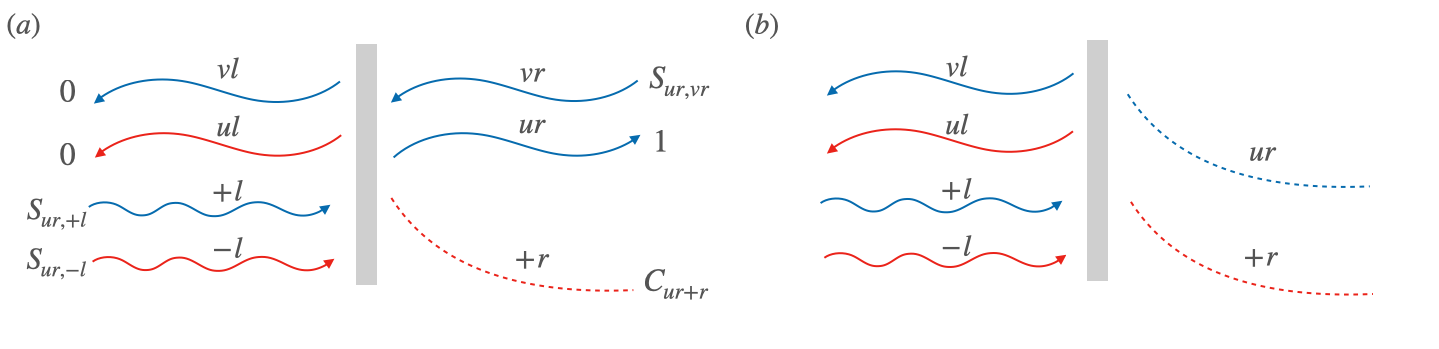
To construct the $ur$ outgoing ($ur$,out) channel in the region $\omega_{\text{min}}<\omega<\omega_{\text{max}}$, one might consider that an outgoing $\phi^{ur}_{p}$ wave with unit amplitude leaves away $x=0$ due to the scattering of the incoming $\phi_{p}^{vr}$ mode moving toward $x=0$ with amplitude $S_{ur,vr}$ in subsonic region, the $\phi^{+l}_{p}$ modes in the supersonic region with $S_{ur,+l}$, and $\phi^{-l}_{p}$ in a particular negative norm state with $S_{ur,-l}$, as shown in Fig. 4. In addition, the decaying mode $\phi_{p}^{+r}$ will be also taken into account on the matching calculations. However, in the region $\omega<\omega_{\text{min}}$, the $\phi^{ur}_{p}$ mode becomes a decaying mode with the vanishing amplitude in the asymptotic region so all $S_{ur,+l},S_{ur,-l},S_{ur,vr}$ vanish. According to the above description, the matching equations can be written as

$$\begin{pmatrix}0\\ 0\\ S_{ur,+l}\\ S_{ur,-l}\end{pmatrix}=M_{\text{scat}}\begin{pmatrix}1\\ S_{ur,vr}\\ C_{ur,+r}\\ 0\end{pmatrix},$$ (65)

where we have replaced $C_{j}$ by the specific expression $S_{in,out}$.

Using the result of $M_{\text{scat}}$ given in (49) and (50) one solves easily the system of equations (65). Up to two leading-order terms in the small $\omega$ expansion for $\omega<\omega_{\text{max}}$, to guarantee the unitary relation (55a), we find that

$$S_{ur,-l}= \Bigg{\{}-\frac{\sqrt{2mc_{p,r}\eta_{r}}\left(v^{2}-c_{p,l}^{2}\right){}^{3/4}\sqrt{c_{p,r}^{2}-v^{2}}\left(\sqrt{c_{p,r}^{2}-v^{2}}+i\sqrt{v^{2}-c_{p,l}^{2}}\right)}{\left(c_{p,r}^{2}-c_{p,l}^{2}\right)\left(c_{p,r}+v\eta_{r}\right)}\frac{1}{\sqrt{\omega}}\,$$

$$+\left[2\sqrt{2m}v\left(c_{p,r}^{2}-c_{p,l}^{2}\right)\left(v^{2}-c_{p,l}^{2}\right){}^{3/4}\left(c_{p,r}^{2}-v^{2}\right)\left(c_{p,r}+v\eta_{r}\right)\right]^{-1}$$

$$\times\sqrt{{c_{p,r}\eta_{r}}\omega}\,\bigg{[}2v^{6}+v^{4}\left(c_{p,r}^{2}-4c_{p,l}^{2}\right)+2v^{2}\left(2c_{p,l}^{4}+c_{p,r}^{4}-3c_{p,l}^{2}c_{p,r}^{2}\right)+c_{p,l}^{4}c_{p,r}^{2}$$

$$-i\Sigma\left(v^{2}-c_{p,l}^{2}\right)\left(c_{p,r}^{2}+2v^{2}\right)\bigg{]}+\mathcal{O}(\omega^{3/2})\Bigg{\}}\theta(\omega-\omega_{r}),$$ (66)

$$S_{ur,vr}=\Bigg{[}\frac{v\eta_{r}-c_{p,r}}{c_{p,r}+v\eta_{r}}\,+\mathcal{O}(\omega^{3/2})\Bigg{]}\theta(\omega-\omega_{r}),$$ (67)

$$S_{ur,+l}= \Bigg{\{}\frac{\sqrt{2mc_{p,r}\eta_{r}}\left(v^{2}-c_{p,l}^{2}\right){}^{3/4}\sqrt{c_{p,r}^{2}-v^{2}}\left(\sqrt{c_{p,r}^{2}-v^{2}}-i\sqrt{v^{2}-c_{p,l}^{2}}\right)}{\left(c_{p,r}^{2}-c_{p,l}^{2}\right)\left(c_{p,r}+v\eta_{r}\right)}\frac{1}{\sqrt{\omega}}\,$$

$$+\left[2\sqrt{2m}v\left(c_{p,r}^{2}-c_{p,l}^{2}\right)\left(v^{2}-c_{p,l}^{2}\right){}^{3/4}\left(c_{p,r}^{2}-v^{2}\right)\left(c_{p,r}+v\eta_{r}\right)\right]^{-1}$$

$$\times\sqrt{{c_{p,r}\eta_{r}}\omega}\,\bigg{[}2v^{6}+v^{4}\left(c_{p,r}^{2}-4c_{p,l}^{2}\right)+2v^{2}\left(2c_{p,l}^{4}+c_{p,r}^{4}-3c_{p,l}^{2}c_{p,r}^{2}\right)+c_{p,l}^{4}c_{p,r}^{2}$$

$$+i\Sigma\left(v^{2}-c_{p,l}^{2}\right)\left(c_{p,r}^{2}+2v^{2}\right)\bigg{]}+\mathcal{O}(\omega^{3/2})\Bigg{\}}\theta(\omega-\omega_{r}),$$ (68)

where $\eta_{r}=\sqrt{1-\omega_{r}^{2}/\omega^{2}}$, $\Sigma=\sqrt{(v^{2}-c_{p,l}^{2})(c_{p,r}^{2}-v^{2})}$, and $\omega_{r}$ is the minimum frequency $\omega_{\text{min}}$ (37).

Figure 5: The Hawking spectrum $n_{p\,\omega}^{ur}$ varies as a function of $\omega$ (in the unit of $mc_{p,l}^{2}$) with different Rabi frequencies: $\Omega/\rho_{0}U_{l}=0.0$ (red), $3.3\times 10^{-4}$ (blue) and $6.6\times 10^{-4}$ (green). The solid lines are based on the numerical computation with details stated in the text, while dashed lines are due to the analytical prediction in (69). We consider $m_{p,l}=7/5,\,m_{p,r}=3/4$, with $U_{r}/U_{l}=8/3,\,U_{AB}/U_{l}=1/3$.

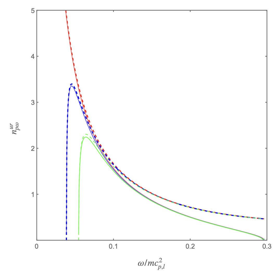
These scattering coefficients can also be obtained numerically from the matching equations (65) together with the normalization condition (27). Those scattering coefficients will be used as the inputs to numerically produce Figs. 5 and 8. Moreover, in these analytical expressions, the step function $\theta(\omega-\omega_{r})$ is added in each equation, when $\omega<\omega_{r}(=\omega_{\text{min}})$ all the modes of the subsonic (upstream) region will become decaying or growing waves. The growing modes are ignored and the decaying modes can not reach the asymptotic region $x\rightarrow\infty$. One expects that particle production occurs in the region ($x<0$) as a result of encountering the total reflection at $x=0$.

To realize the radiation due to particle production from the negative norm states, we first consider the particle distribution function $n_{p\,\omega}^{ur}=\langle 0_{in}|\hat{b}_{\omega}^{ur\dagger}\hat{b}_{\omega}^{ur}|0_{in}\rangle$. We then apply the relations in (53), where the mode mixing occurs in the $ur$ outgoing channel from the negative norm states $\phi_{p}^{-l}$, to give $n_{p\,\omega}^{ur}=|S_{ur,-l}|^{2}$, yielding

$$n_{p\,\omega}^{ur}=|S_{ur,-l}|^{2}=\left[\frac{2mc_{p,r}\eta_{r}\left(v^{2}-c_{p,l}^{2}\right)^{3/2}\left(c_{p,r}^{2}-v^{2}\right)}{\left(c_{p,r}^{2}-c_{p,l}^{2}\right)\left(c_{p,r}+v\eta_{r}\right){}^{2}}\frac{1}{\omega}-\frac{2c_{p,r}v\eta_{r}}{(c_{p,r}+v\eta_{r})^{2}}+\mathcal{O}(\omega)\right]\theta(\omega-\omega_{r})\,.$$ (69)

The $\phi_{p}^{ur}$ modes are called the Hawking modes. The small $\omega$ expansion of the particle distribution function of the Hawking radiation satisfies the Planck distribution

$$\frac{\Gamma}{\exp{\left(\frac{\omega}{T_{H}}\right)}-1},$$ (70)

accompanying by the gray-body factor $\Gamma$ Anderson et al. (2014); Fabbri et al. (2016); Coutant and Weinfurtner (2018); Belgiorno et al. (2020) approximated as

$$\Gamma\left(\frac{T_{H}}{\omega}-\frac{1}{2}+\cdots\right).$$ (71)

Then the effective Hawking temperature and its gray-body factor can be read off from the small $\omega$ expansion of (69) in terms of Mach numbers (31) as follows Larré and Pavloff (2013)

$$T_{H}=\frac{mc_{p,r}^{2}\left(1-m_{p,r}^{2}\right)m_{p,r}^{2}\left(m_{p,l}^{2}-1\right)^{3/2}}{2m_{p,l}\left(m_{p,l}^{2}-m_{p,r}^{2}\right)},$$ (72)

$$\Gamma=\frac{4m_{p,r}\eta_{r}}{\left(1+m_{p,r}\eta_{r}\right)^{2}}.$$ (73)

The effective temperature is monotonically decreased as $m_{p,r}$ ($m_{p,l}$) increases (decreases) toward unity. Especially $T_{H}\rightarrow 0$ as $m_{p,r}\rightarrow 1$ or/and $m_{p,l}\rightarrow 1$ where the analogous horizon disappears. As for the gray-body factor, the relation $\Gamma=1-|S_{ur,vr}|^{2}$ is justified showing that some flux of the particles moves through $x=0$ from the subsonic regime. As compared with the gray-body factor of the gapless cases by sending $\omega_{r}\rightarrow 0$ giving $\eta_{r}\rightarrow 1$ Anderson et al. (2014); Coutant and Weinfurtner (2018)

$$\Gamma_{\omega_{r}=0}=\frac{4m_{p,r}}{(1+m_{p,r})^{2}}.$$ (74)

Here in (73) of the gapped cases the Mach numbers seem to be dressed by the parameters $\eta_{l/r}$ becoming frequency dependent. But these effective Mach numbers have no effects to the Hawking temperature. In particular, when $\omega\rightarrow\omega_{r}$, $\eta_{r}\rightarrow 0$ leads to the gray-body factor $\Gamma\rightarrow 0$ consistent with Balbinot et al. (2019). This is just the critical value of frequency, below which the excitations in the supersonic regime move toward $x=0$ and then are totally reflected away from $x=0$, leading to no Hawking radiation to be observed in the subsonic regime. Thus, for $\omega<\omega_{{r}}$, all $S_{ur,+l},\,S_{ur,-l},\,S_{ur,vr}$ vanish.

III.4 $ul$ outgoing channel

Figure 6: Schematic representation of $ul$, out-channel scattering processes when $\omega_{\text{r}}<\omega<\omega_{\text{max}}$ in (a) and $\omega<\omega_{r}$ in (b).

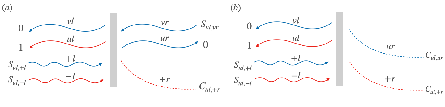
We now discuss the $ul$ outgoing channel in the downstream region of $x<0$, which reveals information about the $\phi_{p}^{ul}$ modes, the partner modes of the Hawking radiations. The $ul$ outgoing channel involves the mode $\phi_{p}^{ul}$ of the negative norm state with the unit amplitude plus three incoming modes, namely $\phi_{p}^{-l}$ with the amplitude $S_{ul,-l}$, $\phi_{p}^{+l}$ with the amplitude $S_{ul,+l}$, and $\phi_{p}^{vr}$ with the amplitude $S_{ul,vr}$ as shown in Fig. 6. The decay mode $\phi_{p}^{+r}$ with the amplitude $C_{ul,+r}$ is included also in this calculation. Now the matching equations become

$$\begin{pmatrix}1\\ 0\\ S_{ul,+l}\\ S_{ul,-l}\end{pmatrix}=M_{\text{scat}}\begin{pmatrix}0\\ S_{ul,vr}\\ C_{ul,+r}\\ 0\end{pmatrix}.$$ (75)

As before we solve the scattering coefficients for $\omega<\omega_{\text{max}}$ in the small $\omega$ expansion

$$S_{ul,-l}= -\frac{\sqrt{m\left(c_{p,r}^{2}-v^{2}\right)}\left(v^{2}-c_{p,l}^{2}\right){}^{3/4}\left(c_{p,r}\eta_{l}+c_{p,l}\eta_{r}\right)\left(\sqrt{c_{p,r}^{2}-v^{2}}+i\sqrt{v^{2}-c_{p,l}^{2}}\right)}{\sqrt{2\,c_{p,l}\eta_{l}\,\omega}\left(c_{p,r}^{2}-c_{p,l}^{2}\right)\left(c_{p,r}+v\eta_{r}\right)}$$

$$+\left[4\sqrt{2}\sqrt{m}v\left(c_{p,r}^{2}-c_{p,l}^{2}\right)\left(v^{2}-c_{p,l}^{2}\right){}^{3/4}\left(c_{p,r}^{2}-v^{2}\right)\sqrt{c_{p,l}\,\eta_{l}}\left(c_{p,r}+v\eta_{r}\right)\right]^{-1}$$

$$\times\sqrt{\omega}\Big{\{}c_{p,r}\left[-2vc_{p,l}\left(c_{p,l}^{2}-c_{p,r}^{2}\right){}^{2}+\eta_{l}\left(v^{2}-c_{p,l}^{2}\right)\left(c_{p,r}^{2}+2v^{2}\right)\left(-c_{p,l}^{2}-i\Sigma+v^{2}\right)\right]$$

$$+\eta_{r}\left[-2v^{3}\eta_{l}\left(c_{p,l}^{2}-c_{p,r}^{2}\right){}^{2}+c_{p,l}\left(c_{p,l}^{2}-v^{2}\right)\left(c_{p,r}^{2}+2v^{2}\right)\left(c_{p,l}^{2}+i\Sigma-v^{2}\right)\right]\Big{\}}$$

$$+\mathcal{O}(\omega^{3/2})\,,$$ (76)

$$S_{ul,vr}= \frac{v\eta_{l}-c_{p,l}}{c_{p,r}+v\eta_{r}}\sqrt{\frac{c_{p,r}\eta_{r}}{c_{p,l}\eta_{l}}}\,\theta(\omega-\omega_{r})+\mathcal{O}(\omega^{3/2}),$$ (77)

$$S_{ul,+l}= \frac{\sqrt{m\left(c_{p,r}^{2}-v^{2}\right)}\left(v^{2}-c_{p,l}^{2}\right){}^{3/4}\left(c_{p,r}\eta_{l}+c_{p,l}\eta_{r}\right)\left(\sqrt{c_{p,r}^{2}-v^{2}}-i\sqrt{v^{2}-c_{p,l}^{2}}\right)}{\sqrt{2\,c_{p,l}\eta_{l}\,\omega}\left(c_{p,r}^{2}-c_{p,l}^{2}\right)\left(c_{p,r}+v\eta_{r}\right)}$$

$$+\left[4\sqrt{2}\sqrt{m}v\left(c_{p,r}^{2}-c_{p,l}^{2}\right)\left(v^{2}-c_{p,l}^{2}\right){}^{3/4}\left(c_{p,r}^{2}-v^{2}\right)\sqrt{c_{p,l}\,\eta_{l}}\left(c_{p,r}+v\eta_{r}\right)\right]^{-1}$$

$$\times\sqrt{\omega}\Big{\{}c_{p,r}\left[-2vc_{p,l}\left(c_{p,l}^{2}-c_{p,r}^{2}\right){}^{2}+\eta_{l}\left(v^{2}-c_{p,l}^{2}\right)\left(c_{p,r}^{2}+2v^{2}\right)\left(-c_{p,l}^{2}+i\Sigma+v^{2}\right)\right]$$

$$+\eta_{r}\left[-2v^{3}\eta_{l}\left(c_{p,l}^{2}-c_{p,r}^{2}\right){}^{2}+c_{p,l}\left(v^{2}-c_{p,l}^{2}\right)\left(c_{p,r}^{2}+2v^{2}\right)\left(-c_{p,l}^{2}+i\Sigma+v^{2}\right)\right]\Big{\}}$$

$$+\mathcal{O}(\omega^{3/2})\,,$$ (78)

where $\eta_{l}=\sqrt{1+\omega_{l}^{2}/\omega^{2}}$, and $\omega_{l}=m_{\text{eff},l}\sqrt{(v^{2}-c_{p,l}^{2})/c_{p,l}^{2}}$. In particular, when $\omega<\omega_{r}$ the $\phi_{p}^{vr}$ mode turns out to be growing modes to be ignored giving the vanishing $S_{ul,vr}$. These coefficients satisfy the unitary relation (55b).

The number density $n_{{p\,-\omega}}^{ul}=\langle 0_{in}|\hat{b}_{-\omega}^{ul\dagger}\hat{b}_{-\omega}^{ul}|0_{in}\rangle$ for the partner modes of the Hawking radiations is

$$n_{p\,-\omega}^{ul}= |S_{ul,+l}|^{2}+|S_{ul,vr}|^{2}$$

$$= \frac{\left(m_{p,l}\eta_{l}+m_{p,r}\eta_{r}\right){}^{2}}{m_{p,l}\eta_{l}\left(1+m_{p,r}\eta_{r}\right){}^{2}}\left(\frac{T_{H}}{\omega}-\frac{1+m_{p,l}\eta_{l}\,m_{p,r}\eta_{r}}{2\left(m_{p,l}\eta_{l}+m_{p,r}\eta_{r}\right)}\right)+\frac{m_{p,r}\eta_{r}\left(1-m_{p,l}\eta_{l}\right)^{2}}{m_{p,l}\eta_{l}\left(1-m_{p,r}\eta_{r}\right)^{2}}\,\theta(\omega-\omega_{r})$$

$$+\mathcal{O}(\omega)\hskip 213.39566pt\qquad\text{for}\qquad\omega_{r}<\omega\leq\omega_{\text{max}}$$ (79)

$$=\left(\frac{m_{p,l}^{2}\eta_{l}^{2}+m_{p,r}^{2}|\eta_{r}|^{2}}{m_{p,l}\eta_{l}+m_{p,l}\eta_{l}m_{p,r}^{2}|\eta_{r}|^{2}}\right)\frac{T_{H}}{\omega}+\frac{\sqrt{m_{p,l}^{2}-1}\,m_{p,r}^{2}|\eta_{r}|\left(m_{p,l}^{2}\eta_{l}^{2}-1\right)}{2\sqrt{1-m_{p,r}^{2}}\,m_{p,l}^{2}\eta_{l}\left(m_{p,r}^{2}|\eta_{r}|^{2}+1\right)}-\frac{1}{2}+\mathcal{O}(\omega)$$

$$\hskip 284.52756pt\text{for}\qquad 0<\omega\leq\omega_{\text{r}}\,.$$ (80)

Since $\phi_{p}^{ul}$ mode itself is the negative norm states with the mode mixing of the incoming modes of the positive norm states, namely, the $\phi_{p}^{+l},\,\phi_{p}^{vr}$ modes, we then write the particle density $n_{{p\,-\omega}}^{ul}$ in terms of the Hawking temperature $T_{H}$ obtained above. Note that both $|S_{ul,+l}|^{2}$ and $|S_{ul,vr}|^{2}$ can not be cast into the Planck distribution in the small $\omega$ expansion leading to the nonthermal nature of $n_{{p\,-\omega}}^{ul}$, the result also found in the work Balbinot et al. (2019). In general, $|S_{ul,vr}|^{2}\ll|S_{ul,+l}|^{2}$. The above features are also true in the gapless cases by setting $\eta_{l}=\eta_{r}=1$.

III.5 $vl$ outgoing channel

Figure 7: Schematic representation of $vl$, out-channel scattering processes when $\omega_{{r}}<\omega<\omega_{\text{max}}$ in (a), and $\omega<\omega_{{r}}$ in (b).

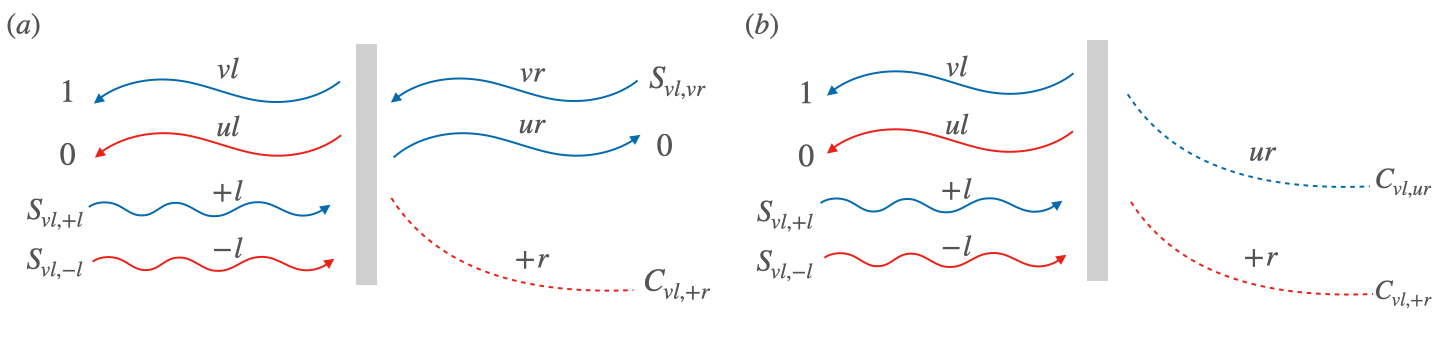
Finally we compute the $vl$ outgoing channel of the positive-norm $\phi_{p}^{vl}$ mode with unit amplitude plus incoming modes, which are $\phi_{p}^{-l}$ of the negative norm state with the amplitude $S_{vl,-l}$, $\phi_{p}^{+l}$ with the amplitude $S_{vl,+l}$, and $\phi_{p}^{vr}$ with the amplitude $S_{vl,vr}$ (see Fig. 7). The corresponding matching equations are

$$\begin{pmatrix}0\\ 1\\ S_{vl,+l}\\ S_{vl,-l}\end{pmatrix}=M_{\text{scat}}\begin{pmatrix}0\\ S_{vl,vr}\\ C_{vl,+r}\\ 0\end{pmatrix},$$ (81)

giving the following scattering coefficients

$$S_{vl,-l}= -\frac{\left(v^{2}-c_{p,l}^{2}\right){}^{3/4}\sqrt{m(c_{p,r}^{2}-v^{2})}\left(c_{p,r}\eta_{l}-c_{p,l}\eta_{r}\right)\left(\sqrt{c_{p,r}^{2}-v^{2}}+i\sqrt{v^{2}-c_{p,l}^{2}}\right)}{\sqrt{2{c_{p,l}\eta_{l}}\,\omega}\left(c_{p,r}^{2}-c_{p,l}^{2}\right)\left(c_{p,r}+v\eta_{r}\right)}$$

$$+\left[4\sqrt{2}\sqrt{m}v\left(c_{p,r}^{2}-c_{p,l}^{2}\right)\left(v^{2}-c_{p,l}^{2}\right){}^{3/4}\left(c_{p,r}^{2}-v^{2}\right)\sqrt{c_{p,l}\,\eta_{l}}\left(c_{p,r}+v\eta_{r}\right)\right]^{-1}$$

$$\times\sqrt{\omega}\,\Big{\{}c_{p,r}\left(-2vc_{p,l}\left(c_{p,l}^{2}-c_{p,r}^{2}\right){}^{2}-\eta_{l}\left[v^{2}-c_{p,l}^{2}\right)\left(c_{p,r}^{2}+2v^{2}\right)\left(-c_{p,l}^{2}+i\Sigma+v^{2}\right)\right]$$

$$+\eta_{r}\left[2v^{3}\eta_{l}\left(c_{p,l}^{2}-c_{p,r}^{2}\right){}^{2}+c_{p,l}\left(v^{2}-c_{p,l}^{2}\right)\left(c_{p,r}^{2}+2v^{2}\right)\left(-c_{p,l}^{2}+i\Sigma+v^{2}\right)\right]\Big{\}}+\mathcal{O}(\omega^{3/2}),$$ (82)

$$S_{vl,vr}= \frac{c_{p,l}+v\eta_{l}}{c_{p,r}+v\eta_{r}}\sqrt{\frac{c_{p,r}\eta_{r}}{c_{p,l}\eta_{l}}}\,\theta(\omega-\omega_{r})+\mathcal{O}(\omega^{3/2}),$$ (83)

$$S_{vl,+l}= \frac{\left(v^{2}-c_{p,l}^{2}\right){}^{3/4}\sqrt{m(c_{p,r}^{2}-v^{2})}\left(c_{p,r}\eta_{l}-c_{p,l}\eta_{r}\right)\left(\sqrt{c_{p,r}^{2}-v^{2}}-i\sqrt{v^{2}-c_{p,l}^{2}}\right)}{\sqrt{2{c_{p,l}\eta_{l}}\,\omega}\left(c_{p,r}^{2}-c_{p,l}^{2}\right)\left(c_{p,r}+v\eta_{r}\right)}$$

$$+\left[4\sqrt{2}\sqrt{m}v\left(c_{p,r}^{2}-c_{p,l}^{2}\right)\left(v^{2}-c_{p,l}^{2}\right){}^{3/4}\left(c_{p,r}^{2}-v^{2}\right)\sqrt{c_{p,l}\,\eta_{l}}\left(c_{p,r}+v\eta_{r}\right)\right]^{-1}$$

$$\times\sqrt{\omega}\,\Big{\{}c_{p,r}\left[-2vc_{p,l}\left(c_{p,l}^{2}-c_{p,r}^{2}\right){}^{2}-\eta_{l}\left(v^{2}-c_{p,l}^{2}\right)\left(c_{p,r}^{2}+2v^{2}\right)\left(-c_{p,l}^{2}-i\Sigma+v^{2}\right)\right]$$

$$+\eta_{r}\left[2v^{3}\eta_{l}\left(c_{p,l}^{2}-c_{p,r}^{2}\right){}^{2}+c_{p,l}\left(c_{p,l}^{2}-v^{2}\right)\left(c_{p,r}^{2}+2v^{2}\right)\left(c_{p,l}^{2}+i\Sigma-v^{2}\right)\right]\Big{\}}$$

$$+\mathcal{O}(\omega^{3/2})\,,$$ (84)

Figure 8: The spectrums of $n_{p\,-\omega}^{ul}$ in (a) and $n_{p\,\omega}^{vl}$ in (b) vary as a function of $\omega$ (in units of $mc_{p,l}^{2}$) with different Rabi frequencies: $\Omega/\rho_{0}U_{l}=0.0$ (red), $3.3\times 10^{-4}$ (blue) and $6.6\times 10^{-4}$ (green). The analytical predictions drawn as dashed lines are obtained from (79)-(80) and (85) while the numerical results, whose details are stated in the text, are presented with solid lines. The parameters are the same as that used in Fig. 5.

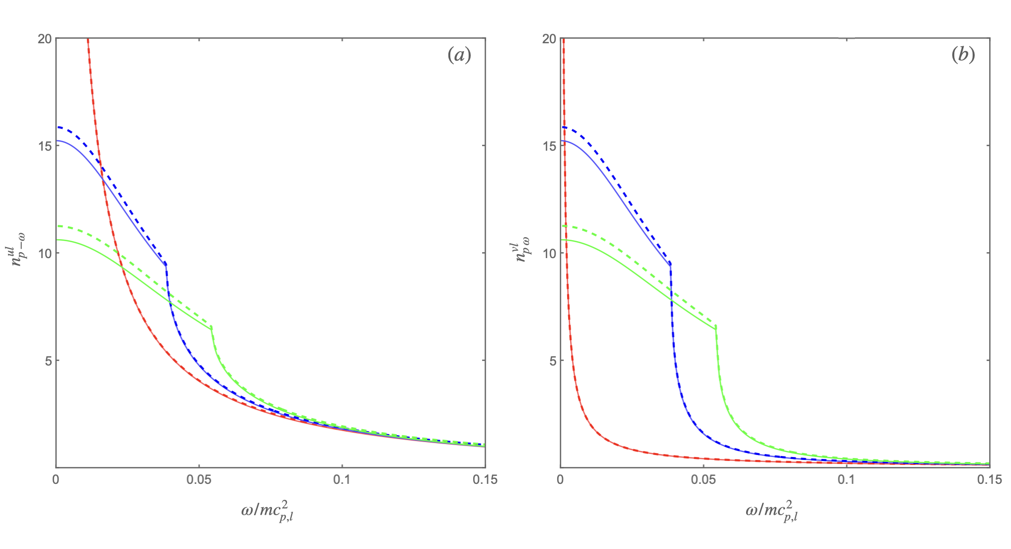
which obey the unitary relation (55c). The particle density $n_{p\,\omega}^{vl}$ defined as $\langle 0_{in}|\hat{b}_{\omega}^{vl\dagger}\hat{b}_{\omega}^{vl}|0_{in}\rangle$ turns out to be

$$n_{p\,\omega}^{vl}=|S_{vl,-l}|^{2}$$ (85)

due to the mode mixing from the negative norm state $\phi_{p}^{-l}$. Another consistency check comes from the fact that $n_{p\,-\omega}^{ul}-n_{p\,\omega}^{vl}=n_{p\,\omega}^{ur}$, given by the current conservation requirement in (59). When $\omega<\omega_{r}=\omega_{\text{min}}$, since there is no Hawking radiation emission $n_{p\,\omega}^{ur}=0$, then $n_{p\,-\omega}^{ul}=n_{p\,\omega}^{vl}$. Once the frequency is larger than $\omega_{r}$, the emergence of Hawking radiation will drastically decrease production of $n_{p\,\omega}^{vl}$. See Fig. 8-($b$) for detail.

IV Density-density correlations

Density-density correlation functions of the gapped excitations can assess the analog Hawking radiation by measuring the correlation between modes in the supersonic and subsonic regimes. The approximate expressions of scattering coefficients for each outgoing channels obtained in the last section can help realize the density-density correlation function. To proceed, the density and the associated phase operators can be defined in terms of the fields $\hat{\phi}_{s}$ and $\hat{\phi}_{s}^{\dagger}$ as

$$\delta\hat{n}_{s}=\frac{\delta\hat{\rho}_{s}}{2\rho_{s}}=\frac{\hat{\phi_{s}}+\hat{\phi}^{\dagger}_{s}}{2},\quad\delta\hat{\theta}_{s}=\frac{\hat{\phi}_{s}-\hat{\phi}_{s}^{\dagger}}{2i},\qquad s=d,p.$$ (86)

Then the density fluctuation operator for the gapped excitations can be expanded as

$$\delta\hat{n}_{p}(x,t)= \int_{\omega_{\text{max}}}^{\infty}d\omega\left[\hat{b}_{\omega}^{ur,out}\chi_{p}^{ur,out}(x,t)+\hat{b}_{\omega}^{vl,out}\chi_{p}^{vl,out}(x,t)\right]$$

$$+\int_{\omega_{\text{min}}}^{\omega_{\text{max}}}d\omega\left[\hat{b}_{\omega}^{ur,out}\chi_{p}^{ur,out}(x,t)+\hat{b}_{\omega}^{vl,out}\chi_{p}^{vl,out}(x,t)+(\hat{b}_{-\omega}^{ul,out})^{\dagger}\chi_{p}^{ul,out}(x,t)\right],$$

$$+\int_{0}^{\omega_{\text{min}}}d\omega\left[\hat{b}_{\omega}^{vl,out}\chi_{p}^{vl,out}(x,t)+(\hat{b}_{-\omega}^{ul,out})^{\dagger}\chi_{p}^{ul,out}(x,t)\right]$$

$$+\text{h.c.},$$ (87)

where

$$\chi_{p}^{j}=(\phi_{p}^{j}+\varphi_{p}^{j})/2$$ (88)

have the formulas given in (44) and (47) according to different out basis. The equal-time correlation function is defined as

$$G_{p}(x,x^{\prime})= \langle 0_{in}|\{\delta\hat{n}_{p}(t,x),\delta\hat{n}_{p}(t,x^{\prime})\}|0_{in}\rangle,$$ (89)

where we consider $in$-vacuum initial state, and $\{\,,\,\}$ is the anticommutation bracket. Employing the Bogoliubov transforms  (53), (58), we have (89) written as

$$\langle\{\delta\hat{n}_{p}(x,t),\,\delta\hat{n}_{p}(x^{\prime},t)\}\rangle_{\omega}$$

$$={\left(|S_{ur,vr}|^{2}+|S_{ur,+l}|^{2}+|S_{ur,-l}|^{2}\right)}\,\chi_{p}^{{ur},out}(x)\chi_{p}^{{ur},out\ast}(x^{\prime})$$

$$\quad+{\left(|S_{vl,vr}|^{2}+|S_{vl,+l}|^{2}+|S_{vl,-l}|^{2}\right)}\,\chi_{p}^{{vl},out}(x)\chi_{p}^{{vl},out\ast}(x^{\prime})$$

$$\quad+{\left(|S_{ul,vr}|^{2}+|S_{ul,+l}|^{2}+|S_{ul,-l}|^{2}\right)}\,\chi_{p}^{ul,out}(x)\chi_{p}^{ul,out\ast}(x^{\prime})$$

$$\quad+{\left(S_{ur,vr}S_{ul,vr}^{\ast}+S_{ur,+l}S_{ul,+l}^{\ast}+S_{ur,-l}S_{ul,-l}^{\ast}\right)}\left(\chi_{p}^{ur,out}(x)\chi_{p}^{ul,out\ast}(x^{\prime})+\chi_{p}^{ur,out}(x^{\prime})\chi_{p}^{ul,out\ast}(x)\right)$$

$$\quad+{\left(S_{ur,vr}S_{vl,vr}^{\ast}+S_{ur,+l}S_{vl,+l}^{\ast}+S_{ur,-l}S_{ul,-l}^{\ast}\right)}\left(\chi_{p}^{ur,out}(x)\chi_{p}^{vl,out\ast}(x^{\prime})+\chi_{p}^{ur,out}(x^{\prime})\chi_{p}^{vl,out\ast}(x)\right)$$

$$\quad+{\left(S_{ul,vr}S_{vl,vr}^{\ast}+S_{ul,+l}S_{vl,+l}^{\ast}+S_{ul,-l}S_{vl,-l}^{\ast}\right)}\left(\chi_{p}^{ul,out}(x)\chi_{p}^{vl,out\ast}(x^{\prime})+\chi_{p}^{ul,out}(x^{\prime})\chi_{p}^{vl,out\ast}(x)\right)$$

$$\quad+\text{c.c.}.$$ (90)

In the end, we will sum over all possible Fourier frequencies $\omega$.

Figure 9: The density-density correlation function pattern is obtained from numerical computations of the integral (89) with the scattering coefficients, wave numbers and mode amplitudes also numerically obtained with the details stated in the text. We have used the parameters $m_{p,l}=7/5,\,m_{p,r}=3/4$, and $\Omega/\rho_{0}U_{l}=6.6\times 10^{-4}$.

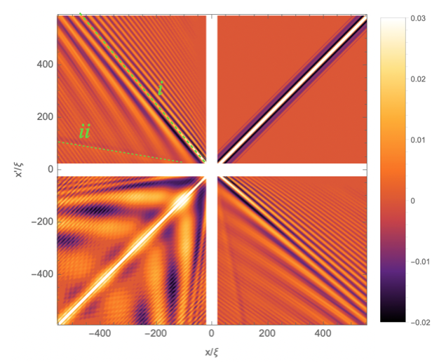
In Fig. 9, we present the full numerical result of the correlation function at equal time, which has the same pattern as in paper Dudley et al. (2018). Our result can be compared with the pattern of the density-density correlation function of the gapless excitations in Recati et al. (2009); Larré and Pavloff (2013). The upper-right quadrant $x>0,x^{\prime}>0$ reveals the correlation of the right-moving positive norm modes $\phi_{p}^{ur}$ with themselves, which shows a clear peak along $x=x^{\prime}$ line, and the correlations vanish when $x\neq x^{\prime}$ due to the atom-atom repulsive interactions. This peak pattern of the gapped excitation is almost the same as for the gapless excitation. The major difference in the density correction function is manifested in the other three quadrants discussed separately below.

IV.1 The quadrant of correlation function within $x<0,x^{\prime}>0$ or $x>0,x^{\prime}<0$

For $x>0,\,x^{\prime}<0$, the density-density correlation function $G_{p}(x,x^{\prime})$ involves the correlations of the right-moving positive norm modes $\phi_{p}^{ur}$ outside the horizon at $x^{\prime}>0$ and the left-moving negative norm modes $\phi_{p}^{ul}$ inside the horizon at $x<0$ as well as the left-moving positive norm modes $\phi_{p}^{vl}$ also inside the horizon at $x<0$. Apart from the peaks along the two lines denoted by $i$ and $ii$ respectively in Fig. 9, which appear in both gapped and gapless cases Recati et al. (2009); Dudley et al. (2018); Larré and Pavloff (2013), the ripples are found in the region below the line $i$ Dudley et al. (2018); Coutant et al. (2012). The pattern of $G_{p}(x,x^{\prime})$ in the quadrant $x<0,x^{\prime}>0$ is the same as in the quadrant $x>0,x^{\prime}<0$ according to the symmetry along the diagonal line $x=x^{\prime}$.

The lines of the peaks and the ripples can be analytically studied as follows. Applying (66) and (76) to (IV) and collecting the relevant terms in the region of $x<0,x^{\prime}>0$, the equal-time correlation function of the upper-left quadrant turns out to be

$$G_{p}(x<0,x^{\prime}>0)=$$

$$\qquad\int_{\omega_{\text{min}}}^{\omega_{\text{max}}}d\omega\,\left[2S_{ur,-l}S_{ul,-l}^{\ast}\chi_{p}^{ur,out}(x^{\prime})\chi_{p}^{ul,out\ast}(x)+2S_{ur,-l}S_{vl,-l}^{\ast}\chi_{p}^{ur,out}(x^{\prime})\chi_{p}^{vl,out\ast}(x)\right]$$

$$\qquad\qquad\qquad+\text{c.c.}$$

$$\qquad\sim\int_{\omega_{\text{min}}}^{\omega_{\text{max}}}d\omega\bigg{[}\frac{m_{p,r}^{2}\left(m_{p,l}\eta_{l}+1\right)\left(m_{p,l}\eta_{l}+m_{p,r}\eta_{r}\right)\sqrt{m_{p,l}^{2}-1}}{4\pi\rho_{0}v\eta_{l}\left(m_{p,l}^{2}-m_{p,r}^{2}\right)\left(m_{p,r}\eta_{r}+1\right)}\,\cos{\left(k_{ul}x-k_{ur}x^{\prime}\right)}$$

$$\qquad\qquad\qquad\qquad\qquad-\frac{m_{p,r}^{2}\left(m_{p,l}\eta_{l}-1\right)\left(m_{p,l}\eta_{l}-m_{p,r}\eta_{r}\right)\sqrt{m_{p,l}^{2}-1}}{4\pi\rho_{0}v\eta_{l}\left(m_{p,l}^{2}-m_{p,r}^{2}\right)\left(m_{p,r}\eta_{r}+1\right)}\,\cos{\left(k_{vl}x-k_{ur}x^{\prime}\right)}\bigg{]}\,.$$ (91)

Here the lines $i,\,ii$ can be determined by the above integral evaluated at $\omega=\omega_{\text{max}}$. One can approximate the integrand with $\eta_{r}=\eta_{l}=1$ in  (91) as $\omega\rightarrow\omega_{\text{max}}$ and then consider the integral at $\omega_{\text{max}}$ to find

$$G_{p}(x<0,x^{\prime}>0)\sim \frac{\left(m_{p,l}+1\right)m_{p,r}^{2}\sqrt{m_{p,l}^{2}-1}}{4\pi\rho_{0}v\left(m_{p,r}+1\right)\left(m_{p,l}-m_{p,r}\right)}\frac{\sin\left[\omega_{\text{max}}\left(\frac{x}{v-c_{p,l}}+\frac{x^{\prime}}{c_{p,r}-v}\right)\right]}{\left(\frac{x}{v-c_{p,l}}+\frac{x^{\prime}}{c_{p,r}-v}\right)}$$

$$-\frac{\left(m_{p,l}-1\right)m_{p,r}^{2}\sqrt{m_{p,l}^{2}-1}}{4\pi\rho_{0}m_{p,l}\left(m_{p,r}+1\right)\left(m_{p,l}+m_{p,r}\right)}\frac{\sin\left[\omega_{\text{max}}\left(\frac{x}{v+c_{p,l}}+\frac{x^{\prime}}{c_{p,r}-v}\right)\right]}{\left(\frac{x}{v+c_{p,l}}+\frac{x^{\prime}}{c_{p,r}-v}\right)}.$$ (92)

The peaks occur in the lines,

$$i\qquad\Rightarrow\qquad\frac{x}{v-c_{p,l}}=-\frac{x^{\prime}}{c_{p,r}-v},$$

$$ii\qquad\Rightarrow\qquad\frac{x}{v+c_{p,l}}=-\frac{x^{\prime}}{c_{p,r}-v},$$

which are attributed to the correlations of $\phi_{p}^{ul}-\phi_{p}^{ur}$ modes ( the line $i$) and $\phi_{p}^{vl}-\phi_{p}^{ur}$ modes (the line $ii$), respectively. The same formula for determining the line $i$ is found for the gapless cases in Mayoral et al. (2011) as long as $\omega_{\text{max}}\gg\omega_{l,r}$ leading to the gapless results Muñoz de Nova et al. (2019). The line $ii$ is also obtained. In particular, the magnitude of the density correlations along the line $i$ is much larger than that in the line of $ii$, which is shown in Fig. 9 and also in Dudley et al. (2018) for the gapped cases, and in Recati et al. (2009); Dudley et al. (2018); Larré and Pavloff (2013) for the gapless cases.

The pattern reveals the ripples in the region of $\frac{x}{v-c_{p,l}}<-\frac{x^{\prime}}{c_{p,r}-v}$ to be realized by studying the phase $\theta=k_{ul}x-k_{ur}x^{\prime}$ ($\theta=k_{vl}x-k_{ur}x^{\prime}$) of the integrand of the first (second) term in (91) as a function of $\omega$. At the points of this region, the phase $\theta$ decreases with $\omega$ as $\omega$ starts from the lower limit of the integral, namely $\omega_{r}$, and then increases instead with $\omega$ as $\omega$ reaches $\omega_{\text{max}}$, developing the local minimum of $\theta$, around which values of $\omega$ give significant contributions to the respective integral (91). The wavelength of the ripples can be estimated from the minimum value of the phase $\theta$ along the lines with the slops $\frac{v-c_{p,l}}{c_{p,r}-v}$ and $\frac{v+c_{p,l}}{c_{p,r}-v}$, which are perpendicular to $i$, $ii$ giving respectively

$$\lambda_{i}= \big{\{}2\pi vm_{p,l}\left(1-m_{p,l}^{2}\right)\left(m_{p,r}-1\right)^{2}\left(m_{p,r}+1\right)\}/\{m_{p,l}^{2}\left(m_{p,r}-1\right)^{2}\left(m_{p,r}+1\right)\sqrt{\omega_{l}^{2}+\omega_{r}^{2}}$$

$$+\omega_{r}\left[2m_{p,l}^{3}m_{p,r}^{3}-m_{p,l}^{2}m_{p,r}^{2}\left(m_{p,l}+m_{p,r}\right)-m_{p,l}m_{p,r}\left(m_{p,l}^{2}+m_{p,r}^{2}\right)+m_{p,l}^{3}+m_{p,r}^{3}\right]\big{\}},$$ (93a)

$$\lambda_{ii}= \big{\{}2\pi vm_{p,l}\left(1-m_{p,l}^{2}\right)\left(m_{p,r}-1\right)^{2}\left(m_{p,r}+1\right)\}\{m_{p,l}^{2}\left(m_{p,r}-1\right)^{2}\left(m_{p,r}+1\right)\sqrt{\omega_{l}^{2}+\omega_{r}^{2}}$$

$$+\omega_{r}\left[2m_{p,l}^{3}m_{p,r}^{3}-m_{p,l}^{2}m_{p,r}^{2}\left(m_{p,l}-m_{p,r}\right)-m_{p,l}m_{p,r}\left(m_{p,l}^{2}+m_{p,r}^{2}\right)+m_{p,l}^{3}-m_{p,r}^{3}\right]\big{\}}.$$ (93b)

In general $\lambda_{ii}<\lambda_{i}$ can be seen in Fig. 9, and both wavelengths are inversely proportional to $\omega_{l}$ and $\omega_{r}$. However, in the region of $\frac{x}{v-c_{p,l}}>-\frac{x^{\prime}}{c_{p,r}-v}$ ripples disappeared because both phases $\theta=k_{ul}x-k_{ur}x^{\prime}$ and $\theta=k_{vl}x-k_{ur}x^{\prime}$ monotonically decrease with $\omega$ that lead to the phase cancellation when integrated over $\omega$.

IV.2 The quadrant of correlation function within $x<0,x^{\prime}<0$

In the lower-left quadrant of $x<0,x^{\prime}<0$, the density correlations account for the negative norm mode $\phi_{p}^{ul}$ and the positive norm mode $\phi_{p}^{vl}$ in the supersonic regime. The correlation pattern shows a cone shape of the group of the peaks in Fig. 9, where a similar behavior also appears in the gapless cases Muñoz de Nova et al. (2019). However, for the gapped cases, again the peculiar pattern of the undulations due to the existence of the zero-frequency modes are also shown as in the paper Dudley et al. (2018). To understand the origin, notice that the density correlation function obtained from the relevant terms of (IV) in the region of $x<0,x^{\prime}<0$ is

$$G_{p}(x<0,x^{\prime}<0)=$$

$$\int_{0}^{\omega_{\text{max}}}d\omega\Big{\{}\left(1+2|S_{vl,-l}|^{2}\right)\chi_{p}^{{vl},out}(x)\chi_{p}^{{vl},out\ast}(x^{\prime})+{\left(1+2|S_{ul,vr}|^{2}+2|S_{ul,+l}|^{2}\right)}\chi_{p}^{ul,out}(x)\chi_{p}^{ul,out\ast}(x^{\prime})$$

$$\qquad\qquad\quad+2\,S_{ul,-l}S_{vl,-l}^{\ast}\left[\chi_{p}^{ul,out}(x)\chi_{p}^{vl,out\ast}(x^{\prime})+\chi_{p}^{ul,out}(x^{\prime})\chi_{p}^{vl,out\ast}(x)\right]$$

$$\qquad\qquad\quad+\text{c.c.}\Big{\}}\,,$$ (94)

where the first line contributes the peaks mainly along the line of $x=x^{\prime}$, and again due to the atom-atom repulsive interaction the correlation vanishes when $x\neq x^{\prime}$. The second line manifests the correlations of the $\phi^{ul}$ and $\phi^{vl}$ modes expressed explicitly in terms of the mode functions $\phi$ and $\varphi$ through (88) by

$$\sim\int_{0}^{\omega_{\text{max}}}d\omega\, \frac{m_{p,l}\left(1-m_{p,r}^{2}\right)\left(m_{p,l}^{2}\eta_{l}^{2}+1\right)\left(m_{p,l}^{2}\eta_{l}^{2}-m_{p,r}^{2}|\eta_{r}|^{2}\right)}{8\pi\rho_{0}v\eta_{l}^{2}\sqrt{m_{p,l}^{2}-1}\left(m_{p,l}^{2}-m_{p,r}^{2}\right)\left(m_{p,r}\eta_{r}+1\right){}^{2}}$$

$$\hskip 56.9055pt\times\left[\cos{\left(k_{ul}x-k_{vl}x^{\prime}\right)}+\cos{\left(k_{ul}x^{\prime}-k_{vl}x\right)}\right],$$ (95)

where the magnitude is given by inserting the scattering coefficients in (76) and (82). Thus the cone shape boundary of the two lines can be determined by evaluating the above integral at its upper limit $\omega_{\text{max}}$. In this case, because $\omega_{\text{max}}\gg\omega_{l,r}$ where $\eta_{l,r}\rightarrow 1$ is considered, the integral evaluated at the upper limit leads to the similar formula as in (IV.1), giving the two lines to be

$$\frac{x}{m_{p,l}-1}=\frac{x^{\prime}}{m_{p,l}+1},\quad\text{and}\quad\frac{x}{m_{p,l}+1}=\frac{x^{\prime}}{m_{p,l}-1},$$ (96)

which are the same as in the gapless cases in Recati et al. (2009). The magnitude of the density correlations on the two lines are the same. The slopes of the lines ($i$ and $ii$) only depend on $m_{p,l}$ since both modes are at $x<0,x^{\prime}<0$. The increasing $m_{p,l}$ can increase the effective temperature $T_{H}$ in (72) but decrease the angle of cone, namely, reducing the area of the undulations confined in the cone.

The undulations, which show up only for the gapped cases, can be understood analytically as follows. Their typical wavelength $\lambda$ near the direction of $x=x^{\prime}$ can be extracted directly form the phase $\theta=k_{ul}x-k_{vl}x^{\prime}$ in the region of small $\omega$ given by

$$\lambda\simeq\frac{2\pi}{(k_{ul}-k_{vl})}\Big{|}_{\omega=0}\simeq\frac{\pi(v^{2}-c_{p,l}^{2})}{c_{p,l}\omega_{l}},$$ (97)

which is consistent with Fig. 9. The zero-frequency modes in the solutions of the momentum $k_{v}$ and $k_{u}$ in (38) and (39) in the supersonic region for the gapped cases play a key role in determining the wavelength of the undulations. The phase $\theta$ outside the cone decreases monotonically with $\omega$ that leads to the phase cancellation when integrating over $\omega$ so that the undulations disappear.

V Quantum entanglement between Hawking modes and its partners

V.1 The PHS criterion

This section devotes to the discussion of quantum entanglement in this system. We first briefly introduce the criterion of the quantum entanglement between the Hawking mode and its partner. The quantum entanglement and/or the nonseparability of the bipartite systems can be explored based upon the PHS criterion Peres (1996); Horodecki et al. (1996); Horodecki (1997); Simon (2000), which then is adapted to assess the entanglement through the simple measure Busch and Parentani (2014)

$$\Delta^{ur,ul}_{p\,\omega}=n_{p\,\omega}^{ur}n_{p\,-\omega}^{ul}-|c^{ur,ul}_{p\,\omega}|^{2}.$$ (98)

The formula uses the particle number density $n_{\omega}$ and their cross correlations defined as

$$c^{ur,ul}_{p\,\omega}=\langle 0_{in}|\hat{b}_{\omega}^{ur,out}\hat{b}_{-\omega}^{ul,out}|0_{in}\rangle=S_{ur,vr}S_{ul,vr}^{\ast}+S_{ur,+l}S_{ul,+l}^{\ast}=S_{ur,-l}S_{ul,-l}^{\ast}\,.$$ (99)

Here we consider the pair modes of the positive norm state $\phi^{ur}$, the analogous Hawking mode in the subsonic regime, and the negative norm state $\phi^{ul}$, the partner mode in the supersonic regime. Using the unitary properties of the $S$-matrix, the measure then becomes

$$\Delta^{ur,ul}_{p\,\omega}=-|S_{ur,-l}|^{2}\,.$$ (100)

Apparently, the values of $\Delta_{\omega}^{ur,ul}$ are always negative implying that two modes are quantum mechanical entanglement. The above discussions hold true for both gapless and gapped excitations.

Here is the side issue about how the nonzero particle number distribution for the incoming modes in the subsonic regime affects the entanglement of the Hawking mode and its partner Coutant and Weinfurtner (2018). It is quite straightforward to generalize the above formulas by considering the incoming $\phi_{p}^{vr}$ mode with the nonzero particle distribution function $n_{p\,\omega}^{vr,in}$. In the gapped cases, it reads

$$\Delta^{ur,ul}_{{{p}}\,\omega}=\left(|S_{ul,vr}|^{2}-|S_{ur,-l}|^{2}\right)n_{p\,\omega}^{vr,in}-|S_{ur,-l}|^{2},\qquad\omega>\omega_{r}\,,$$ (101)

which can be rewritten as

$$\frac{\Delta^{ur,ul}_{{{p}}\,\omega}}{|S_{ur,-l}|^{2}}=\delta_{ur,ul}n_{p\,\omega}^{vr,in}-1$$ (102)

with

$$\delta_{ur,ul}= \frac{|S_{ul,vr}|^{2}-|S_{ur,-l}|^{2}}{|S_{ur,-l}|^{2}}=\frac{\left(m_{p,l}\eta_{l}-m_{p,r}\eta_{r}\right)^{2}}{4m_{p,l}\eta_{l}m_{p,r}\eta_{r}}.$$ (103)

In (103), $\delta_{ur,ul}$ is always positive, and thus can not possibly be set to vanishing since $m_{p,l},\eta_{l}>1$ in the supersonic region and $m_{p,r},\eta_{r}<1$ in the subsonic region. $\delta_{ur,ul}$ can be tuned to zero so as to avoid the reduction of entanglement in the gapless cases ($\eta_{l,r}\rightarrow 1$) under the condition of $v_{l}c_{l}=v_{r}c_{r}$ Coutant and Weinfurtner (2018).

V.2 Inhomogeneous equations

As for the quantum entanglement in the BEC systems, which are affected by the omnipresent environment, there have been extensive studies in various fluctuating environmental degrees of freedom Adamek et al. (2013); Busch and Parentani (2013); Robertson and Parentani (2015); Lang et al. (2020). Here the binary systems have the parameter window to turn on the interactions between gapless and gapped excitations. More specifically, we would like to study how the gapped excitations treated as an environment affect the quantum entanglement between the Hawking modes and their partners of the gapless excitations. This is an extension of our previous work in Syu et al. (2019), where the gapped excitations serve as the environmental degrees of freedom to induce the sound cone fluctuations, the analogous light cone fluctuations given by the quantum gravitational effects. To turn on the interactions, we relax the restriction of the parameters to have small difference between two intra-species interaction $U_{AA}$, $U_{BB}$ while other restrictions such as $\rho_{l}=\rho_{r}=\rho_{0}$, $v_{l}=v_{r}={-v\,(v>0)}$, $\Omega_{l}=\Omega_{r}=\Omega$ still hold. Then, the interaction between gapless and gapped excitations starts at $t=0$ with the interaction term

$$\mathcal{L}_{\text{int}}=-\alpha\rho_{0}^{2}\delta\hat{n}_{p}\delta\hat{n}_{d}\,.$$ (104)

The interaction strength $\alpha$ is given by

$$\alpha=({U}_{AA}-{U}_{BB})\theta(t).$$ (105)

We assume that two degrees of freedom are completely decoupled when $t<0$, and establish their own excitations under the super-subsonic configuration, namely $c_{{s},l}<v<c_{s,r}$ for $s=d,p$. After turning on the interaction, the gapped excitations start to influence the quantum entanglement of the pair modes of the gapless excitations, resulting in the time dependent $\Delta_{\omega}^{jj^{\prime}}$ developed above. The coupled equations of motion for $\delta\hat{n}_{d}$ of the gapless excitations and $\delta\hat{n}_{p}$ of the gapped excitations defined in (86), which can be adapted from (17)-(18) by including the above interaction term, are obtained as

$$\left(\partial_{t}-v\partial_{x}\right)^{2}\delta\hat{n}_{d}+\frac{1}{2m}\partial_{x}^{2}\left(\frac{1}{2m}\partial_{x}^{2}-2mc_{d}^{2}\right)\delta\hat{n}_{d}=\frac{\alpha\rho_{0}}{2m}\partial_{x}^{2}\delta\hat{n}_{p},$$ (106)

$$\left(\partial_{t}-v\partial_{x}\right)^{2}\delta\hat{n}_{p}+\frac{1}{2m}\partial_{x}^{2}\left(\frac{1}{2m}\partial_{x}^{2}-2mc_{p}^{2}\right)\delta\hat{n}_{p}+m_{\text{eff}}^{2}\delta\hat{n}_{p}=\frac{\alpha\rho_{0}}{2m}(\partial_{x}^{2}-2m\Omega)\delta\hat{n}_{d}\,.$$ (107)

Thus, the general solution of (106) is the sum of two parts, the homogeneous solution $\delta n_{d,0}$ and the inhomogeneous solution $\delta n_{d1}$, namely

$$\delta\hat{n}_{d}(x,t)=\delta\hat{n}_{d,0}(x,t)+\delta\hat{n}_{d,1}(x,t).$$ (108)

The homogeneous solution $\delta n_{d,0}$ obeying the source-free equation (106) is very much the same as in the gapped excitations with the mode expansion (87), where the creation/annihilation operators and also the mode functions are replaced by the counterparts denoted by ${\hat{a}_{\omega}^{\dagger}}/\hat{a}_{\omega}$ and $\chi_{d}(x,t)$ defined as in (88) and obtained from (20) and (28). The wave number $k_{d}$ of the gapless cases for each incoming/outgoing modes are those in (39) and (40) by setting $m_{\text{eff}}=0$ and replacing $c_{p(l,r)}$ by $c_{d(l,r)}$. The maximum wave number of the gapless case for having the negative norm states in the downstream at $x<0$ is found to be $k_{\text{max}}^{\scriptscriptstyle(0)}$ in (33), again by replacing $c_{p(l,r)}$ to $c_{d(l,r)}$. The threshold momentum turns out to be zero for the gapless cases. In the end, the density-density correlations used later to identify the quantities $n_{\omega}^{j}$ and $c_{\omega}^{jj^{\prime}}$, with which to compute the criterion $\Delta_{\omega}^{jj^{\prime}}$ in (98) in the gapless cases, will have the same form as in (IV). All the $S$-matrix elements in the gapless case are those of the gapped cases in (66)-(68) for the $ur$ outgoing channel, (76)-(78) for the $ul$ outgoing channel, and (82)-(84) for the $vl$ outgoing channel by taking the limit of $m_{\text{eff}}=0$ and replacing $c_{p(l,r)}$ by $c_{d(l,r)}$.

On the other hand, the inhomogeneous solution $\delta n_{d\,1}$ obeys the Eq. (106) due to the source term from $\delta n_{p}$, which is the solution of (107). The solution of $\delta n_{p}$ can also be written as the homogeneous solution $\delta n_{p0}$ and the inhomogeneous solution that depends linearly on $\delta n_{d\,1}$. According to Boyanovsky and Jasnow (2017); Syu et al. (2021), substituting the solution $\delta n_{p}=\delta n_{p\,0}+\delta n_{p\,1}$ back to the Eq. (106) of $\delta n_{d\,1}$ gives the damping term from the contribution of $\delta n_{p\,1}$ and leaves $\delta n_{p\,0}$ in the right-hand side of the equation as a source term. Since the interaction term of the gapless and gapped excitations involves second order spatial derivatives, the damping effect of the momentum dependence can be parametrized as

$$\gamma(k)=(\alpha\rho_{0})^{2}[k^{2}(k^{2}+2m\Omega)/4m^{2}]/2m_{\text{eff}}^{3}$$ (109)

Busch and Parentani (2013). In the hydrodynamical approximation with small $k$ and $\omega$, the relevant parameter from the gapped excitations to the damping term is $m_{\text{eff}}$, giving the correct dimension of $\gamma$. Here we will focus on the saturated value of $\Delta_{\omega}^{jj^{\prime}}$ whereas the effect of the damping term damps out the oscillatory time-dependent terms, leading to saturation. The relaxation time scales can be estimated from $1/\gamma$. Strictly speaking, the effects from the gapped excitations to the gapless degrees of freedom can be obtained by integrating out the gapped excitations as in Syu et al. (2019). This then leads to the Langevin equation that takes into account not only the fluctuations of the gapped excitations manifested in the noise term but also the damping effect. This deserves future studies.

So, the fluctuations of the gapped degrees of freedom will give the corrections to the density-density correlation function of the gapless excitations through the solution of $\delta\hat{n}_{d,1}$ due to the source term $\delta\hat{n}_{p,0}$

$$\delta\hat{n}_{d,1}(x,t)=\int_{-\infty}^{\infty}dx^{\prime}\int_{-\infty}^{\infty}dt^{\prime}\,g_{\text{ret}}(x,t,x^{\prime},t^{\prime})\,\frac{\alpha\rho_{0}}{2m}\partial_{x^{\prime}}^{2}\delta\hat{n}_{p,0}(x^{\prime},t^{\prime})\,.$$ (110)

The Fourier transform of the retarded Green’s function is defined as

$$g_{\text{ret}}(x,t;x^{\prime},t^{\prime})=\int\frac{d\omega}{2\pi}\frac{dk}{2\pi}\,\,\tilde{g}_{\text{ret}}(\omega,k)e^{-i\omega(t-t^{\prime})}e^{ik(x-x^{\prime})}$$ (111)

with the solution

$$\tilde{g}_{\text{ret}}({\omega},{k})=\frac{-1}{\left({\omega+v_{0}{k}}\right)^{2}+2i\gamma(k)\omega-c_{d}^{2}{k}^{2}-{k}^{4}/4m^{2}}\,,$$ (112)

which includes the damping effect. The inhomogeneous solution for the small wave number consistent with the hydrodynamical approximation lying within $\gamma<vk$ becomes

$$\delta\hat{n}_{d,1}(x,t)= \frac{\alpha\rho_{0}i}{2m}\int dx^{\prime}dt^{\prime}\theta(t^{\prime})\theta(t-t^{\prime})$$

$$\times\int\frac{d{k}}{2\pi}\left[\frac{e^{-i({\omega}_{d\,-}(k)-i\gamma(k))(t-t^{\prime})}-e^{-i({\omega}_{d\,+}(k)-i\gamma(k))(t-t^{\prime})}}{{\omega}_{d\,-}(k)-{\omega}_{d\,+}(k)}\right]e^{i{k}(x-x^{\prime})}\,\partial_{x^{\prime}}^{2}\delta\hat{n}_{p,0}(x^{\prime},t^{\prime}),$$ (113)

where, ${\omega}_{d\,-,+}$ are given by

$$\omega_{d\,-}(k)\equiv-v\,k-\sqrt{c_{d}^{2}\,k^{2}+k^{4}/4m^{2}},$$ (114a)

$$\omega_{d\,+}(k)\equiv-v\,k+\sqrt{c_{d}^{2}\,k^{2}+k^{4}/4m^{2}}\,.$$ (114b)

The frequencies $\omega_{d\,-}$ and $\omega_{d\,+}$ are obtained from the dispersion relation (21) of the gapless excitations of the negative and positive frequencies branches, respectively. Substituting the mode expansion of $\delta\hat{n}_{p,0}$ expressed in (87) and integrating over the space, time and also the wave number, we end up with the formula

$$\delta\hat{n}_{d,1}(x,t)= \int_{\omega_{\text{max}}}^{\infty}d{\omega}\{\,\hat{b}_{\omega}^{ur,out}w_{+}^{ur}+\hat{b}_{\omega}^{vl,out}w_{+}^{vl}\}$$

$$+\int_{\omega_{\text{min}}}^{\omega_{\text{max}}}d{\omega}\{\,\hat{b}_{\omega}^{ur,out}w_{+}^{ur}+(\hat{b}_{-\omega}^{ul,out})^{\dagger}w_{+}^{ul}+\hat{b}_{\omega}^{vl,out}w_{+}^{vl}\}$$

$$+\int_{0}^{\omega_{\text{min}}}d{\omega}\{\,(\hat{b}_{-\omega}^{ul,out})^{\dagger}w_{+}^{ul}+\hat{b}_{\omega}^{vl,out}w_{+}^{vl}\}$$

$$+\text{H.c.},$$ (115)

where we have defined the effective mode functions

$$w_{+}^{j}(x,t)= -\frac{\alpha\rho_{0}}{2m}\,\left(\frac{1-e^{-\gamma[k_{j}]}e^{-i({\omega}_{d\,-}[{k}_{j}]-{\omega})t}}{({\omega}_{d\,-}[{k}_{j}]-i\gamma[k_{j}]-{\omega})}-\frac{1-e^{-\gamma[k_{j}]}e^{-i(\omega_{d\,+}[{k}_{j}]-{\omega})t}}{(\omega_{d\,+}[{k}_{j}]-i\gamma[k_{j}]-{\omega})}\right)$$ (116a)

$$\times\frac{{k}_{j}^{2}}{\Delta\omega_{d\,\pm}[{k}_{j}]}\,\chi_{p}^{j,out}(x,t),$$

$$w_{-}^{j}(x,t)= -\frac{\alpha\rho_{0}}{2m}\,\left(\frac{1-e^{-\gamma[-k_{j}]}e^{-i({\omega}_{d\,-}[-{k}_{j}]+{\omega})t}}{{\omega}_{d\,-}[-{k}_{j}]-i\gamma[-k_{j}]+\omega}-\frac{1-e^{-\gamma[-k_{j}]}e^{-i({\omega}_{d\,+}[-{k}_{j}]+{\omega})t}}{\omega_{d\,+}[-{k}_{j}]-i\gamma[-k_{j}]+\omega}\right)$$

$$\times\frac{(-{k}_{j})^{2}}{\Delta\omega_{d\,\pm}[-{k}_{j}]}\,\chi_{p}^{j,out\ast}(x,t)$$ (116b)

with

$$\Delta\omega_{d\,\pm}[k_{j}]={\omega}_{d\,-}[{k}_{j}]-\omega_{d\,+}[{k}_{j}]=-2\sqrt{c_{d}^{2}{k}_{j}^{2}+{k}_{j}^{4}/4m^{2}}$$

for the channels $j$ including $j=ur,ul,vl$ with the wave number $k_{j}$ of the gapped excitations obtained from a fixed $\omega$. The Green’s function serves as a window function that smears the effect from the gapped excitations to the gapless excitations.

We are now ready to calculate the correlation function of the gapless excitations including the corrections from the gapped excitations for a particular frequency $\omega$

$$G_{d\,\omega}(x,t;x^{\prime},t^{\prime}) =\langle in|\{\delta\hat{n}_{d}(x,t),\delta\hat{n}_{d}(x^{\prime},t^{\prime})\}|in\rangle_{\omega}$$

$$=\langle in|\{\delta\hat{n}_{d,0}(x,t),\delta\hat{n}_{d,0}(x^{\prime},t^{\prime})\}|in\rangle_{\omega}+\langle in|\{\delta\hat{n}_{d,1}(x,t),\delta\hat{n}_{d,1}(x^{\prime},t^{\prime})\}|in\rangle_{\omega}$$

$$=G_{d,\omega\,0}(x,t;x^{\prime},t^{\prime})+G_{d,\omega\,1}(x,t;x^{\prime},t^{\prime}),$$ (117)

where the initial state is given by the in-vacuum state of the gapless and gapped excitations $|in\rangle=|0_{in}\rangle_{\text{gapless}}\otimes|0_{in}\rangle_{\text{gapped}}$. The first term is the correlation function of the unperturbed gapless excitations. This is quite a straightforward calculation to compute $G_{d,\omega\,0}(x,t;x^{\prime},t^{\prime})$ by starting from the mode expansion of the gapless excitations in (15a) where the mode functions are written in (20) in terms of the coefficients in (28). The wave numbers denoted by $k_{d}$ together with the $S$-matrix elements $S^{d}$ associated with the Bogoliubov transformation of the creation/annihilation operators as in (53) can be read off from the gapped excitations in (39) and (40) and the above $S$-matrix elements by replacing $c_{p}\rightarrow c_{d}$ and also setting $m_{\text{eff}}=0$ or $\Omega=0$ limit. The second term comes from the modification due to the gapped excitations. In this study, we consider both gapless and gapped excitations are under the supersonic-subsonic configuration in the monometric in (17)-(18) choosing $\Omega=4\rho_{0}U_{AB}\ll\rho_{0}U$. Also, for small Rabi-coupling $\Omega$ giving small $m_{\text{eff}}\propto\sqrt{\Omega}$ in (25), the sound-speed difference $c_{p}-c_{d}\propto\Omega$ in (22) and (24) is small, and controls the smallness of the wave number difference $k_{j}-k_{d\,j}\propto\Omega\ll 1/\xi$ in various modes. We then can approximate $w_{\pm}^{j}$ in (116) of the gapped excitations by

$$w_{+}^{j}(x,t)\simeq W_{+}^{j}(t)\chi_{d}^{j,out}(x,t)\left[1+i\mathcal{O}\left(x({k}_{j}-k_{d\,j})\right)\right],$$ (118a)

$$w_{-}^{j}(x,t)\simeq W_{-}^{j}(t)\chi_{d}^{j,out}(x,t)\left[1-i\mathcal{O}\left(x({k}_{j}-k_{d\,j})\right)\right],$$ (118b)

where

$$W_{+}^{j}(t)=-\frac{\alpha\rho_{0}}{2m}\left(\frac{A_{p\,k_{j}}+B_{p\,k_{j}}}{A_{d\,k_{j}}+B_{d\,k_{j}}}\right)$$

$$\quad\qquad\qquad\times\left(\frac{1-e^{-\gamma[k_{j}]t}e^{-i({\omega}_{d\,-}[{k}_{j}]-{\omega})t}}{{\omega}_{d\,-}[{k}_{j}]-i\gamma[k_{j}]-{\omega}}-\frac{1-e^{-\gamma[k_{j}]t}e^{-i(\omega_{d\,+}[{k}_{j}]-{\omega})t}}{\omega_{d\,+}[{k}_{j}]-i\gamma[k_{j}]-{\omega}}\right)\frac{{k}_{j}^{2}}{\Delta\omega_{d\,\pm}[{k}_{j}]}\,,$$ (119a)

$$W_{-}^{j}(t)=W_{+}^{j\ast}(t)\,.$$ (119b)

As long as the length scales in the hydrodynamic approximation of our interest are of order of the correlation length $\xi$ or beyond it, it leads to the considerably small error to be ignored safely. Therefore, one can rewrite the functions $\chi_{p}^{j,out}(x,t)$ in (87) of the gapped excitations defined in (88), (20) and (29) in terms of $A_{p\,k_{j}}$ and $B_{p\,k_{j}}$ (29) by the functions $\chi_{d}^{j,out}(x,t)$ of the gapless excitations in terms of $A_{d\,k_{j}}$ and $B_{d\,k_{j}}$ in (28) instead.

According to different quadrants in the $(x,x^{\prime})$ plane, we summarize the correlation functions as follows. For the upper-right quadrant $x>0,x^{\prime}>0$ in the interval $\omega_{\text{min}}<\omega\leq\omega_{\text{max}}$,

$$G_{d\,\omega}(x,x^{\prime};t)\simeq \left[(1+2|{S}^{d}_{ur,-l}|^{2})+(1+2|{S}_{ur,-l}|^{2})W_{+}^{ur}(t)W_{-}^{ur}(t)\right]\chi_{d}^{ur,out}(x,t)\chi_{d}^{ur,out\ast}(x^{\prime},t)$$

$$+\text{c.c.},$$ (120)

and in the interval $0<\omega\leq\omega_{\text{min}}$,

$$G_{d\,\omega}(x,x^{\prime};t)\simeq(1+2{S}^{d}_{ur,-l}|^{2})\chi_{d}^{ur,out}(x,t)\chi_{d}^{ur,out\ast}(x^{\prime},t)+\text{c.c.}.$$ (121)

For the upper-left quadrant $x<0,x^{\prime}>0$ in the interval $\omega_{\text{min}}<\omega\leq\omega_{\text{max}}$,

$$G_{d\,\omega}(x,x^{\prime};t)\simeq \left(2{S}^{d}_{ur,-l}{S}_{ul,-l}^{d\,\ast}+2S_{ur,-l}S_{ul,-l}^{\ast}W_{+}^{ur}(t)W_{-}^{ul}(t)\right){\chi}_{d}^{ur,out}(x^{\prime},t){\chi}_{d}^{ul,out\ast}(x,t)$$

$$\qquad+\left(2{S}^{d}_{ur,-l}{S}_{vl,-l}^{d\,\ast}+2S_{ur,-l}S_{vl,-l}^{\ast}W_{+}^{ur}(t)W_{-}^{vl}(t)\right){\chi}_{d}^{ur,out}(x^{\prime},t){\chi}_{d}^{vl,out\ast}(x,t)$$

$$+\text{c.c.},$$ (122)

and in the interval $0<\omega\leq\omega_{\text{min}}$,

$$G_{d\,\omega}(x,x^{\prime};t)\simeq \left(2{S}^{d}_{ur,-l}{S}_{ul,-l}^{d\,\ast}\right){\chi}_{d}^{ur}(x^{\prime},t){\chi}_{d}^{ul\ast}(x,t)+\left(2{S}^{d}_{ur,-l}{S}_{vl,-l}^{d\,\ast}\right){\chi}_{d}^{ur,out}(x^{\prime},t){\chi}_{d}^{vl,out\ast}(x,t)$$

$$+\text{c.c.}.$$ (123)

Finally, for the lower-right quadrant $x<0,x^{\prime}<0$ in the interval of $\omega_{\text{min}}<\omega\leq\omega_{\text{max}}$,

$$G_{d\,\omega}(x,x^{\prime};t)\simeq \left\{\left[1+2\left(|{S}^{d}_{ul,vr}|^{2}+|{S}^{d}_{ul,+l}|^{2}\right)\right]+\left[1+2\left(|{S}_{ul,vr}|^{2}+|{S}_{ul,+l}|^{2}\right)\right]W_{+}^{ul}(t)W_{-}^{ul}(t)\right\}$$

$$\times{\chi}_{\omega\,d}^{ul,out}(x,t){\chi}_{d}^{ul,out\ast}(x^{\prime},t)+\left[\left(1+2|{S}^{d}_{vl,-l}|^{2}\right)+\left(1+2|{S}_{vl,-l}|^{2}\right)W_{+}^{vl}(t)W_{-}^{vl}(t)\right]$$

$$\times{\chi}_{\omega\,d}^{vl,out}(x,t){\chi}_{d}^{vl,out\ast}(x^{\prime},t)+\text{c.c.},$$ (124)

and in the interval $0<\omega\leq\omega_{\text{min}}$,

$$G_{d\,\omega}(x,x^{\prime};t)\simeq \left\{\left[1+2\left(|{S}^{d}_{ul,vr}|^{2}+|{S}^{d}_{ul,+l}|^{2}\right)\right]+\left(1+2|{S}_{ul,+l}|^{2}\right)W_{+}^{ul}(t)W_{-}^{ul}(t)\right\}$$

$$\times\chi_{d}^{ul,out}(x,t)\chi_{d}^{ul,out\ast}(x^{\prime},t)+\left[\left(1+2|{S}^{d}_{vl,-l}|^{2}\right)+\left(1+2|{S}_{vl,-l}|^{2}\right)W_{+}^{vl}(t)W_{-}^{vl}(t)\right]$$

$$\times\chi_{d}^{vl,out}(x,t)\chi_{d}^{vl,out\ast}(x^{\prime},t)+\text{c.c.}.$$ (125)

V.3 Nonseparability of Hawking-partner pairs

Having gotten the correlation functions, we can extract the effective mean occupation number $1+2{n}_{\omega}^{ur}$ and $1+2{n}_{\omega}^{ul}$ from the correlation functions in $x>0,x^{\prime}>0$ and $x<0,x^{\prime}<0$, and the cross correlation terms $2{c}_{\omega}^{ur,ul}$ from the correlation function in $x<0,x^{\prime}>0$ Busch and Parentani (2013); Robertson and Parentani (2015). For a given frequency of the pair mode of the gapless excitations, due to the bilinear coupling between the gapless and gapped excitations, the corrections from the gapped excitations also come from the modes with frequency $\omega$. Thus, when $\omega_{\text{min}}<\omega\leq\omega_{\text{max}}$

$$n_{d\,\omega}^{ur}=|{S}^{d}_{ur,-l}|^{2}+\left(\,|S_{ur,-l}|^{2}+1/2\right)|W_{+}^{ur}|^{2},$$ (126a)

$$n_{d\,\omega}^{ul}=\left(\,|{S}^{d}_{ul,vr}|^{2}+|{S}^{d}_{ul,+l}|^{2}\right)+\left(\,|S_{ul,vr}|^{2}+|S_{ul,+l}|^{2}+1/2\right)|W_{+}^{ul}|^{2},$$ (126b)

$$c_{d\,\omega}^{ur,ul}={S}^{d}_{ur,-l}{S}_{ul,-l}^{d\,\ast}+S_{ur,-l}S_{ul,-l}^{\ast}W_{+}^{ur}W_{-}^{ul}\,.$$ (126c)

The criterion $\Delta_{d\,\omega}^{ur,ul}$ in (98) can be computed, using the unitary relations of gapless and gapped excitations leads to

$$\Delta_{d\,\omega}^{ur,ul}\simeq -|{S}^{d}_{ur,-l}|^{2}+|{S}^{d}_{ur,-l}|^{2}\left(\frac{1}{2}+|{S}_{ul,+l}|^{2}\right)|W_{+}^{ul}|^{2}+|{S}^{d}_{ul,+l}|^{2}\left(\frac{1}{2}+|{S}_{ur,-l}|^{2}\right)|W_{+}^{ur}|^{2}$$

$$-\left({S}^{d}_{ur,-l}{S}_{ul,-l}^{d\,\ast}S_{ur,-l}S_{ul,-l}^{\ast}W_{+}^{ur}W_{-}^{ul}+\text{c.c.}\right)+\mathcal{O}(|W_{+}^{j}|^{3})\,.$$ (127)

With no influence from the gapped excitations, $\Delta_{d\,\omega}^{ur,ul}$ is negative meaning that the Hawking modes $\phi_{d}^{ur}$ and their partner modes $\phi_{d}^{ul}$ are quantum mechanically entangled. The effects of the gapped excitations contribute the modification of the occupation number density $n_{d\,\omega}^{ur}$ and $n_{d\,\omega}^{ul}$ in (126a) and (126b) that increase the value of $\Delta_{d\,\omega}^{ur,ul}$ diminishing the separability. However, the cross correlation term $|c_{d\,\omega}^{ur,ul}|^{2}$ in (126c) decreases $\Delta_{d\,\omega}^{ur,ul}$ strengthening the entanglement, but its effect is less than that of $n_{d\,\omega}^{ur}$ and $n_{d\,\omega}^{ul}$ due to the relative smallness of the overlap between $W_{+}^{ur}$ and $W_{-}^{ul}$. The net effects of the gapped excitations raise $\Delta_{d\,\omega}^{ur,ul}$, driving the pair modes toward disentanglement.

However, when $0<\omega\leq\omega_{\text{min}}$, since the $\phi^{ur}$ modes of the gapped excitations are not the propagating modes, the modification only acts on $n_{\omega}^{ul}$, while the other two terms remain unaffected. Thus,

$$n_{d\,\omega}^{ur}=|{S}^{d}_{ur,-l}|^{2},$$ (128a)

$$n_{d\,\omega}^{ul}=\left(\,|{S}^{d}_{ul,vr}|^{2}+|{S}^{d}_{ul,+l}|^{2}\right)+\left(\,|S_{ul,+l}|^{2}+1/2\right)|W_{+}^{ul}|^{2},$$ (128b)

$$c_{d\,\omega}^{ur,ul}={S}^{d}_{ur,-l}{S}_{ul,-l}^{d\,\ast}.$$ (128c)

Figure 10: The time evolution of $\Delta_{d,\omega}^{ur,ul}$ as a function of the time in unit of period $T_{\omega}=2\pi/\omega$ with the parameters Mach number $m_{p,r}=0.63,\,m_{p,l}=1.63$, the coupling constant $\alpha/U_{l}=0.13$, the Rabi frequency $\Omega/\rho_{0}U_{l}=6.6\times 10^{-4}$. Considering (a) $\omega=0.041T_{H}<\omega_{\text{min}}=0.157T_{H}$, $\Delta_{d\,\omega}^{ur,ul}$ behaves as an underdamped oscillation, (b) $\omega=0.124T_{H}<\omega_{\text{min}}=0.157T_{H}$ , $\Delta_{d\,\omega}^{ur,ul}$ behaves as an overdamped oscillation, and (c) $\omega=0.16T_{H}>\omega_{\text{min}}=0.157T_{H}$, the behavior of $\Delta_{d\,\omega}^{ur,ul}$ has mixture of overdamped oscillation for $ul$ mode and underdamped oscillation for $ur$ mode. The dashed lines indicate the values of $\Delta_{d,\omega}^{ur,ul}$ with no corrections from the gapped excitations.

Figure 11: Late-time saturation of $\Delta_{d\,\omega}^{ur,ul}$ is plotted as function of $\omega$ in unit of effective temperature $T_{H}$. By varying the Rabi frequency $\Omega/\rho_{0}U_{l}$: (a) $6.6\times 10^{-4}$, (b) $1.33\times 10^{-3}$, and (c) $2\times 10^{-3}$, we show $\Delta_{d\,\omega}^{ur,ul}$ with two different values of the mutual coupling constants $\alpha/U_{l}:$ 0.1 (red-dotted line) and 0.17 (blue-dashed line). Other parameters are chosen as $m_{p,r}=0.63,\,m_{p,l}=1.63$.

The criterion $\Delta_{d\,\omega}^{ur,ul}$ given by (128) becomes

$$\Delta_{d\,\omega}^{ur,ul}\simeq -|{S}^{d}_{ur,-l}|^{2}+|{S}^{d}_{ur,-l}|^{2}\left(\frac{1}{2}+|S_{ul,+l}|^{2}\right)|W_{+}^{ul}|^{2}+\mathcal{O}(|W_{+}^{ul}|^{3})\,$$ (129)

also increasing $\Delta_{d\,\omega}^{ur,ul}$ with the tendency to disentangle the pair of modes.

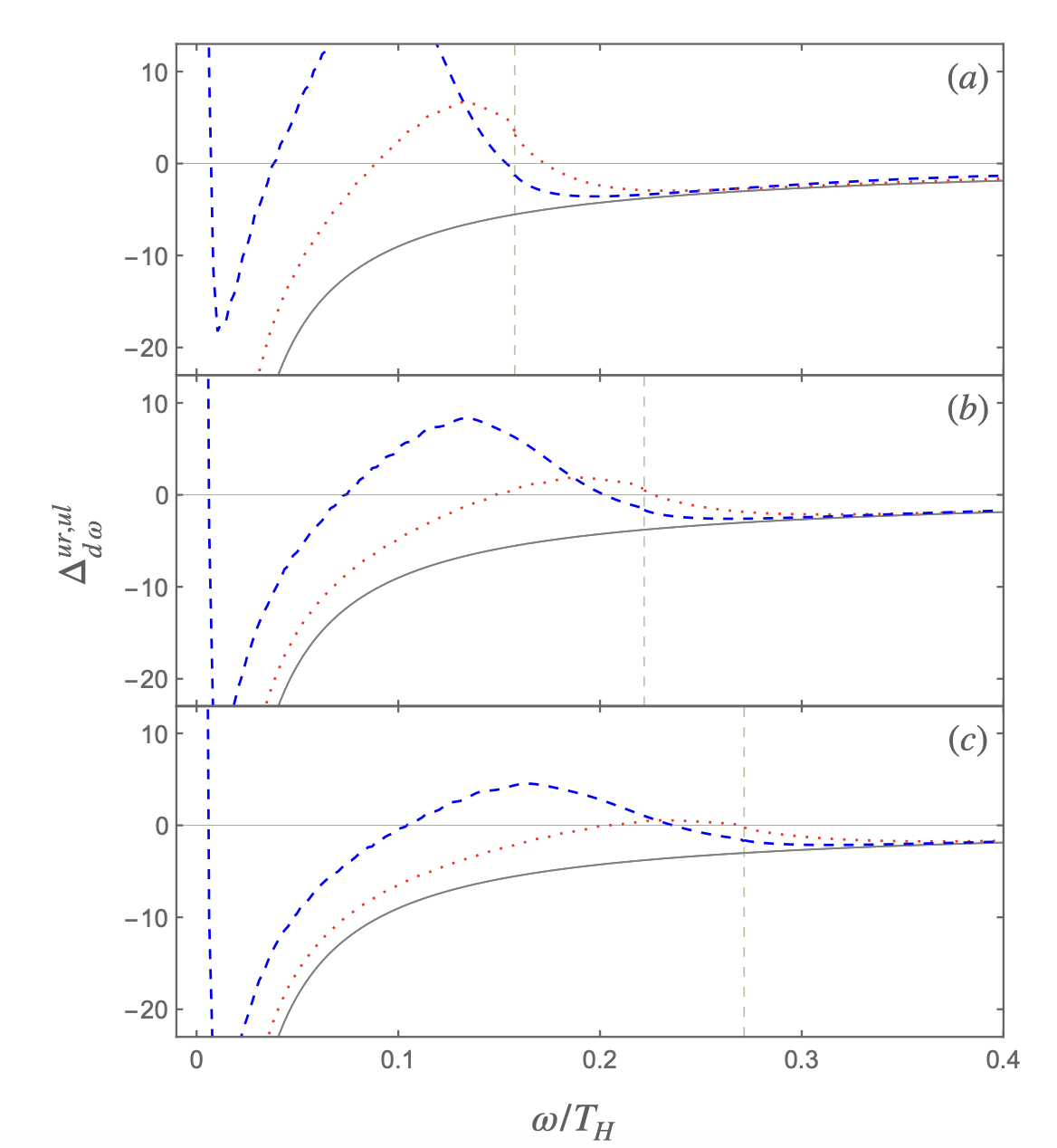
The time evolution of $\Delta_{d\,\omega}^{ur,ul}$ for various values of $\omega$ is plotted in Fig. 10. To understand the behavior, one can approximate $|W_{+}^{ur}|^{2}$ and $|W_{+}^{ul}|^{2}$ from (119) as

$$|W_{+}^{ur}|^{2}\propto\frac{1+e^{-2\gamma[k_{ur}]t}-2e^{-\gamma[k_{ur}]t}\cos{[(\omega-{\omega}_{d\,+}[k_{ur}])}t]}{\gamma^{2}[k_{ur}]+(\omega-{\omega}_{d\,+}[k_{ur}])^{2}}\frac{k_{ur}^{4}}{(\Delta{\omega}_{d\,\pm}[k_{ur}])^{2}},$$ (130a)

$$|W_{+}^{ul}|^{2}\propto\frac{1+e^{-2\gamma[k_{ul}]t}-2e^{-\gamma[k_{ul}]t}\cos{[(\omega-{\omega}_{d\,-}[k_{ul}])}t]}{\gamma^{2}[k_{ul}]+(\omega-{\omega}_{d\,-}[k_{ul}])^{2}}\frac{k_{ul}^{4}}{(\Delta\omega_{d\,\pm}[k_{ul}])^{2}}\,.$$ (130b)

For a given frequency $\omega$, the wave numbers of the Hawking modes and their partners of the gapped excitations $k_{ur}$ and $k_{ul}$ can be given from (39) in the setting of the supersonic-subsonic configuration. For $\omega<\omega_{\text{min}}$, the corrections to $\Delta_{d\,\omega}^{ur,ul}$ in (129) only come from the term $|W_{+}^{ul}|^{2}$. However, when $\omega>\omega_{\text{min}}$, the terms of $W_{+}^{ur}$ and $W_{+}^{ul}$ contributes to the corrections in (127). Due to the fact that the damping factor $\gamma[k_{ul}]>\gamma[k_{ur}]$ for a given $\omega$, the saturation of $\Delta_{d\,\omega}^{ur,ul}$ will take longer time. As for the saturated values in Fig. 11, it is evident that the large corrections occur in frequency that respectively minimize $\gamma^{2}[k_{ur}]+(\omega-{\omega}_{d\,+}[k_{ur}])^{2}$ and $\gamma^{2}[k_{ul}]+(\omega-{\omega}_{d\,-}[k_{ul}])^{2}$ when $\omega\sim\omega_{\text{min}}$ as anticipated. And for large enough value $\alpha$, the behavior of $1/\omega$ in the thermal spectrum $n_{p\,\omega}^{ur}=|S_{ur,-l}|^{2}$ given by (69) will significantly deteriorate the quantum entanglement of the pair modes of the gapless excitations as seen in the expression (129) and Fig. 11.

The presence of the environmental field at finite temperature that deteriorate the quantumness of the pair modes of the gapless excitations in the BEC system has been studied in Busch and Parentani (2014). Here the effects the gapped excitations serving as the environmental degrees of the freedom in two-component BEC systems even though they are in their vacuum states are to provide the stochastic noise that not only induces the sound cone fluctuations in Syu et al. (2019) but also reduces the quantum entanglement of gapless excitation pairs. The similar reduction mechanism on the quantumness of the modes will expectedly be seen in the BEC/BCS crossover models of the ultra-cold Fermi systems as the noise manifested from quantum density fluctuations in condensates of ultra-cold Fermi gases of the gapped modes is found to lead to fluctuations in phonon times-of-flight in the BEC regime Lee et al. (2020).

VI Summary and outlook

We investigate the properties of the condensates of cold atoms at zero temperature in the tunable binary Bose-Einstein condensate system with the Rabi transition between atomic hyperfine states where the system can be represented by a coupled two-field model of gapless excitations and gapped excitations, analogous to the Goldstone modes and the gapped Higgs modes in particle physics. We then set up the configuration of the supersonic and subsonic regimes with the acoustic horizon between them by means of the spatially dependent coupling constant between two hyperfine states in the elongated two-component Bose-Einstein condensates. The aim is to try to mimic Hawking radiations, in particular due to the gapped excitations with the tunable energy-gap term induced by the Rabi-coupling constant. In this work, the simplified steplike sound speed profile is adopted to implement the subsonic-supersonic transition so that such a system be analytically treatable. Two sets of the wave functions of the gapped excitations can be determined by matching them at the acoustic horizon using the obtained dispersion relations. The existence of the negative norm states in the supersonic regime leads to the mixing between the creation operator and the annihilation operator through the Bogoliubov transformation, and thus triggers the particle production, the analog Hawking radiation. The effective-energy gap term in the dispersion relation of the gapped excitations gives a threshold frequency $\omega_{\text{min}}$ in the subsonic regime in the analog Hawking modes, below which the propagating modes do not exist. Thus, the particle spectrum of the corresponding Hawking modes significantly deviates from the gapless cases near the threshold frequency resulting from the modified gray-body factor, which vanishes as the mode frequency is below the threshold frequency. The other feature is that the energy gap term introduces the zero-frequency modes, which leads to the density-density correlation function with the peculiar pattern of the undulations in the supersonic regime. Their wavelength can be determined by the effective-energy gap with cone shaped boundaries depending on the March number of the condensate fluid in the supersonic regime.

The created radiations of the gapped modes will influence the quantumness of the pair of the Hawking mode in the subsonic regime and its partner in the supersonic regime of the gapless excitations by turning on the interactions between the gapless and gapped excitation through tuning their own atomic coupling constants. We consider the limit of the small Rabi-coupling constant giving the small difference in the wave numbers for a given frequency between the gapless and gapped excitations as compared with the inverse of the healing length $\xi$. In the hydrodynamic approximation, the corrections to the density-density correlation function of the gapless excitations due to the gapped excitations can be written in terms of the wave functions of the gapless excitations, resulting in the effective density-density correlation function. Then, from there the effective $S$-matrix elements of the gapless excitations with the corrections from the gapped excitations can be extracted. The measure of the quantum entanglement is according to the PHS criterion to be computed from the obtained effective $S$-matrix elements. The negative value of the PHS measure of the pair modes indicates the nature of the quantum entanglement. It shows that the presence of the gapped excitations created from the $in$-vacuum state, although they are quantum entangled, will significantly deteriorate the quantumness of the pair modes of the gapless excitations created also from the $in$-vacuum state when the frequency of the pair modes is around the threshold frequency, $\omega\sim\omega_{\text{min}}$. On top of that, when the coupling constant between the gapless and gapped excitations becomes large enough, the huge particle density of the gapped excitations in the small $\omega$ regime will significantly disentangle the pair modes of the gapless excitations.

Here the damping term is added from the type of the coupling between the gapless and gapped excitations and can be derived via the influence functional approach following the work of Syu et al. (2019). After integrating out the degrees of freedom of the gapped excitations, the corresponding Langevin equations for describing the gapless excitations can be derived with the damping term and the accompanying noise term that manifests quantum fluctuations of the gapped excitations. One can find the time-dependent PHS measure from which to decode the more precise time scales after which the measure is settled to some final value. Additionally, we may extend our analysis from 1+1 spacetime to 2+1 spacetime, to mimic the effects from the acoustic spinning black holes.