On Feature Learning in Neural Networks with Global Convergence Guarantees

Abstract

We study the optimization of wide neural networks (NNs) via gradient flow (GF) in setups that allow feature learning while admitting non-asymptotic global convergence guarantees. First, for wide shallow NNs under the mean-field scaling and with a general class of activation functions, we prove that when the input dimension is no less than the size of the training set, the training loss converges to zero at a linear rate under GF. Building upon this analysis, we study a model of wide multi-layer NNs whose second-to-last layer is trained via GF, for which we also prove a linear-rate convergence of the training loss to zero, but regardless of the input dimension. We also show empirically that, unlike in the Neural Tangent Kernel (NTK) regime, our multi-layer model exhibits feature learning and can achieve better generalization performance than its NTK counterpart.

1 Introduction

The training of neural networks (NNs) is typically a non-convex optimization problem, but remarkably, simple algorithms like gradient descent (GD) or its variants can usually succeed in finding solutions with low training losses. To understand this phenomenon, a promising idea is to focus on NNs with large widths (a.k.a. under over-parameterization), for which we can derive infinite-width limits under suitable ways to scale the parameters by the widths. For example, under a “$1/\sqrt{\text{width}}$” scaling of the weights, the GD dynamics of wide NNs can be approximated by the linearized dynamics around initialization, and as the widths tend to infinity, we obtain the Neural Tangent Kernel (NTK) limit of NNs, where the solution obtained by GD coincides with a kernel method [37]. Importantly, theoretical guarantees for optimization and generalization can be obtained for wide NNs under this scaling [19, 5]. Nonetheless, it was pointed out that this NTK analysis replies on a form of lazy training that excludes the learning of features or representations [16, 72], which is a crucial ingredient to the success of deep learning, and is therefore not adequate for explaining the success of NNs [27, 41].

Meanwhile, for shallow (i.e., one-hidden-layer) NNs, if we choose a “1 / width” scaling, we can derive an alternative mean-field (MF) limit as the widths tend to infinity. Under this scaling, feature learning occurs even in the infinite-width limit, and the training dynamics can be described by the Wasserstein gradient flow of a probability measure on the space of the parameters, which converges to a global minimizer of the loss function under certain conditions [59, 50, 63, 14]. Generalization guarantees have also been proved for learning with shallow NNs under the MF scaling by identifying a corresponding function space [6, 48]. However, currently there are three limitations to this model of over-parameterized NNs. First, the global convergence guarantees for shallow NNs only hold in the infinite-width limit (i.e. they are asymptotic). While [12] studies the deviation between finite-width NNs and their infinite-width limits during training, the analysis is done only asymptotically to the next order in width. Second, a convergence rate has yet to be established except under special assumptions or with modifications to the GD algorithm [13, 34, 43, 38]. Third, while several works have proposed to extend the MF formulation to deep (i.e., multi-layer) NNs [4, 62, 52, 23, 57], there is less concensus on what the right model should be than for the shallow case. In summary, we still lack a model for the GD optimization of shallow and multi-layer NNs that goes beyond lazy training while admitting fast global convergence.

In this work, we study the optimization of both shallow NNs under the MF scaling and a type of partially-trained multi-layer NNs, and obtain theoretical guarantees of linear-rate global convergence.

1.1 Summary of main contributions

We consider the scenario of training NN models to fit a training set of $n$ data points in dimension $d$, where the model parameters are optimized by gradient flow (GF, which is the continuous-time limit of GD) with respect to the squared loss. Allowing most choices of the activation function, we prove that:

1. For a shallow NN, if the hidden layer is sufficiently wide and the input data are linearly independent (requiring $n\leq d$), then with high probability, the training loss converges to zero at a linear rate.

2. For a multi-layer NN where we only train the second-to-last layer, if the hidden layers are both sufficiently wide, then with high probability, the training loss converges to zero at a linear rate. Unlike for shallow NNs, here we no longer need the requirement on input dimension, demonstrating a benefit of jointly having depth and width.

We also run numerical experiments to demonstrate that our model exhibits feature learning and can achieve better generalization performance than its NTK counterpart.

1.2 Related works

Over-parameterized NNs, NTK and lazy training.

Many recent works have studied the optimization landscape of NNs and the benefits of over-parameterization [24, 67, 60, 66, 64, 54, 65, 42, 3, 40, 76, 15, 75, 17, 39, 9, 32, 20, 31, 61, 10]. One influential idea is the Neural Tangent Kernel (NTK) [37], which characterizes the behavior of GD on the infinite-width limit of NNs under a particular scaling of the parameters (e.g. for shallow NNs, replacing $1/m$ with $1/\sqrt{m}$ in (1)). In particular, when the network width is polynomially large in the size of the training set, the training loss converges to a global minimum at a linear rate under GD [19, 5, 55]. Nonetheless, in the NTK limit, due to a relatively large scaling of the parameters at initialization, the hidden-layer features do not move significantly [37, 19, 16]. For this reason, the NTK scaling has been called the lazy-training regime, as opposed to a feature-learning or rich regime [16, 72, 26]. Several works have investigated the differences between the two regimes both in theory [28, 29, 69, 47] and in practice [27, 41]. In addition, several works have generalized the NTK analysis by considering higher-order Taylor approximations of the GD dynamics or finite-width corrections to the NTK [2, 35, 7, 33].

Mean-field theory of NNs.

An alternative path has been taken to study shallow NNs in the mean-field scaling (as in (1)), where the infinite-width limit is analogous to the thermodynamic or hydrodynamic limit of interacting particle systems [59, 50, 63, 14, 49, 70]. Thanks to the interchangeability of the parameters, the neural network is equivalently characterized by a probability measure on the space of its parameters, and the training can then be described by a Wasserstein gradient flow followed by this probability measure, which, in the infinite-width limit, converges to global mimima under mild conditions. Regarding convergence rate, ref. [71] proves that if we train a shallow NN to fit a Lipschitz target function under population loss, the convergence rate cannot beat the curse of dimensionality. In contrast, we will study the setting of empirical risk minimization, where there are finitely many training data. Ref. [34] shows that mean field Langevin dynamics on shallow NNs can converge exponentially to global minimizers in over-regularized scenarios, but we focus on GF without entropic regularization. Besides the question of optimization, shallow NNs under this scaling represent functions in the Barron space [48] or variation-norm function space [6], which provide theoretical guarantees on generalization as well as fluctuation in training [12]. Several works have proposed different mean-field limits of wide multi-layer NNs and proved convergence guarantees [4, 62, 51, 52, 23, 57, 22], but questions remain. First, due to the presence of different symmetries in a multi-layer network compared to a shallow network [57], the limiting object at the infinite-width limit is often quite complicated. Second, it has been pointed out that under the MF scaling of a multi-layer network, an i.i.d. initialization of the weights would lead to a collapse of the diversity of neurons in the middle layers, diminishing the effect of having large widths [23]. In addition, while another line of work develops MF models of residual models [8, 46, 21, 36], we are interested in multi-layer NN models with a large width in every layer.

Feature learning in deep NNs.

Ref. [1] demonstrates the importance of hierarchical learning by proving the existence of concept classes that can be learned efficiently by a deep NN with quadratic activations but not by non-hierarchical models. Ref. [11] studies the optimization landscape and generalization properties of a hierarchical model that is similar to ours in spirit, where an untrained embedding of the input is passed into a trainable shallow model, and prove an improvement in sample complexity in learning polynomials by having neural network outputs as the embedding. However, the trainable models they consider are not shallow NNs but their linearized and quadratic-Taylor approximations, and furthermore the convergence rate of the training is not known. Ref. [73] proposes a novel parameterization under which there exists an infinite-width limit of deep NNs that exhibits feature learning, but properties of its training dynamics is not well-understood. Our multi-layer NN models adopt an equivalent scaling (see Appendix C), and our focus is on proving non-asymptotic convergence guarantees for its partial training under GF.

2 Problem setup

2.1 Model

We summarize our notations in Appendix A. Let $\Omega\subseteq\mathbb{R}^{d}$ denote the input space, and let $\bm{x}=[x_{1},...,x_{d}]^{\intercal}\in\Omega$ denote a generic input data vector. A shallow NN model under the MF scaling can be written as:

$$f(\bm{x})=\frac{1}{m}\sum_{i=1}^{m}c_{i}\sigma\Big{(}\frac{1}{\sqrt{d}}\sum_{j=1}^{d}W_{ij}x_{j}\Big{)}~{},$$ (1)

where $m$ is the width, $W\in\mathbb{R}^{m\times d}$ and $\bm{c}=[c_{1},...,c_{m}]\in\mathbb{R}^{m}$ are the first- and second-layer weight parameters of the model, and $\sigma:\mathbb{R}\to\mathbb{R}$ is the activation function. For simplicity of presentation, we neglect the bias terms. In this paper, we study a more general type of models with the following form:

$$f(\bm{x})= \frac{1}{m}\sum_{i=1}^{m}c_{i}\sigma\big{(}h_{i}(\bm{x})\big{)}~{},$$ (2)

$$\forall i\in[m]\quad:\quad h_{i}(\bm{x})= \frac{1}{\sqrt{D}}\sum_{j=1}^{D}W_{ij}\phi_{j}(\bm{x})~{},\qquad$$ (3)

where $W\in\mathbb{R}^{m\times D}$ and $\bm{c}=[c_{1},...,c_{m}]\in\mathbb{R}^{m}$ are parameters of the model, and $\phi_{1},...,\phi_{D}$ are a set of functions from $\Omega$ to $\mathbb{R}$ that we call the embedding. Each of $h_{1},...,h_{m}$ is a function from $\Omega$ to $\mathbb{R}$, and we will refer to them as the (hidden-layer) feature map or activations. For simplicity, we write $\Phi(\bm{x})=[\phi_{i}(\bm{x}),...\phi_{D}(\bm{x})]^{\intercal}\in\mathbb{R}^{D}$. We consider two types of the embedding, $\Phi$, as described below:

Fixed embedding

$D$ is fixed and $\Phi$ is deterministic. In the simplest example, we set $D=d$ and $\phi_{j}(\bm{x})=x_{j}$, $\forall j\in[D]$, and recover the shallow NN model in (1). More generally, our definition includes cases where $\Phi$ is a deterministic transformation of an input vector in $\Omega$ into an embedding vector in $\mathbb{R}^{D}$. This can be understood as input pre-processing or feature engineering.

High-dimensional random embedding

$D$ is large and $\Phi$ is random. For instance, we can sample each $\bm{z}_{j}$ i.i.d. in $\mathbb{R}^{d}$ and set $\phi_{j}(\bm{x})=\sigma\Big{(}\frac{1}{\sqrt{d}}\bm{z}_{j}^{\intercal}\bm{x}\Big{)}$, equivalent to setting $\phi_{1},...,\phi_{m}$ as the hidden-layer activations of a shallow NN with randomly-initialized first-layer weights. Then, the model becomes

$$f(\bm{x})= \frac{1}{m}\sum_{i=1}^{m}c_{i}\sigma\big{(}h_{i}(\bm{x})\big{)}~{},$$ (4)

$$\forall i\in[m]\quad:\quad h_{i}(\bm{x})= \frac{1}{\sqrt{D}}\sum_{j=1}^{D}W_{ij}\sigma\Big{(}\frac{1}{\sqrt{d}}\bm{z}_{j}^{\intercal}\bm{x}\Big{)}~{}.$$ (5)

Thus, we obtain a $3$-layer feed-forward NN whose first-layer weights are random and fixed, and we call it a partially-trained $3$-layer (P-$3$L) NN. Note that the scaling in this model is different from both the NTK scaling ($1/\sqrt{m}$ instead of $1/m$ in (4)) and the MF scaling for multi-layer NNs adopted in [4, 62, 51, 57, 23] ($1/{D}$ instead of $1/\sqrt{D}$ in (5)). We show in Appendix B that when $\sigma$ is homogeneous, this scaling is consistent with the Xavier initialization of neural network parameters up to a reparameterization [30, 56]. We also show in Appendix C that in certain cases this scaling is equivalent to the maximum-update parameterization proposed in [73]. Numerical experiments that compare different scalings are described in Section 4.

2.2 Training with gradient flow

Consider the scenario of supervised least-squares regression, where we are given a set of $n$ training data points together with their target values, $(\bm{x}_{1},y_{1}),...,(\bm{x}_{n},y_{n})\in\Omega\times\mathbb{R}$. We fit our models by minimizing the empirical squared loss:

$$\mathcal{L}[f]=\frac{1}{2}\sum_{a=1}^{n}\big{(}f(\bm{x}_{a})-y_{a}\big{)}^{2}~{}.$$ (6)

To do so, we first initialize the parameters randomly by sampling each $c_{i}$ and $W_{ij}$ i.i.d. from probability measures $\pi_{c}\in\mathcal{P}(\mathbb{R})$ and $\pi_{\bm{w}}\in\mathcal{P}(\mathbb{R}^{D})$, respectively, and then perform GD on $W$. For simplicity of analysis, we leave $\bm{c}$ untrained, and further assume that

Assumption 1.

$\pi_{c}=\frac{1}{2}\delta_{\hat{c}}(dc)+\frac{1}{2}\delta_{-\hat{c}}(dc)$ for some $\hat{c}>0$ independent from $m$, which is the law of a scaled Rademacher random variable.

If $\sigma$ is Lipschitz, it is differentiable almost everywhere, and we write $\sigma^{\prime}(\bm{x})$ to denote the derivative of $\sigma$ when it is differentiable at $\bm{x}$ and $0$ otherwise. When $\sigma$ is differentiable at $h_{i}(\bm{x})$, there is

$$\frac{\partial f}{\partial W_{ij}}(\bm{x})=\frac{1}{m\sqrt{D}}c_{i}\sigma^{\prime}\big{(}h_{i}(\bm{x})\big{)}\phi_{j}(\bm{x})~{},$$ (7)

and the gradient of the loss function with respect to $W_{ij}$ is given by

$$\frac{\partial\mathcal{L}[f]}{\partial W_{ij}}= \frac{1}{m\sqrt{D}}c_{i}\sum_{a=1}^{n}\left(f(\bm{x}_{a})-y_{a}\right)\sigma^{\prime}\big{(}h_{i}(\bm{x}_{a})\big{)}\phi_{j}(\bm{x}_{a})~{}.$$ (8)

Thus, we can perform GD updates on $W$ according to the following rule: $\forall i\in[m]$ and $\forall j\in[D]$,

$$W_{ij}\quad\leftarrow\quad W_{ij}-m\delta\frac{\partial\mathcal{L}[f]}{\partial W_{ij}}=W_{ij}-\frac{\delta}{\sqrt{D}}c_{i}\sum_{a=1}^{n}\left(f(\bm{x}_{a})-y_{a}\right)\sigma^{\prime}\big{(}h_{i}(\bm{x}_{a})\big{)}\phi_{j}(\bm{x}_{a})~{},$$ (9)

where $\delta>0$ is the step size. As we discuss in Appendix B, this is consistent with the standard GD update rule for Xavier-initialzed NNs. In the limit of infinitesimal step size ($\delta\to 0$), the evolution of the parameters during training is described by the GF equation: if we use the superscript $t\geq 0$ to denote time elaposed during training, the time-derivative of the parameters is given by

$$\dot{W}_{ij}^{t}=-\frac{c_{i}}{\sqrt{D}}\sum_{a=1}^{n}\left(f^{t}(\bm{x}_{a})-y_{a}\right)\sigma^{\prime}\big{(}h_{i}^{t}(\bm{x}_{a})\big{)}\phi_{j}(\bm{x}_{a})~{},$$ (10)

where $f^{t}$ denotes the output function and $h_{1}^{t},...,h_{m}^{t}$ denote the hidden-layer feature maps determined by the parameters at time $t$. Then, induced by the evolution of $W^{t}$, each $h_{i}^{t}$ evolves according to

$$\forall\bm{x}\in\Omega\quad:\quad\dot{h}_{i}^{t}(\bm{x})= \frac{1}{\sqrt{D}}\sum_{j=1}^{D}\dot{W}_{ij}^{t}\phi_{j}(\bm{x})=-{c_{i}}\sum_{a=1}^{n}\mathcal{G}(\bm{x},\bm{x}_{a})\left(f^{t}(\bm{x}_{a})-y_{a}\right)\sigma^{\prime}\big{(}h_{i}^{t}(\bm{x}_{a})\big{)}~{},$$ (11)

where we define a kernel function $\mathcal{G}:{\Omega}\times\Omega\to\mathbb{R}$ as

$$\mathcal{G}(\bm{x},\bm{x}^{\prime})=\frac{1}{D}\sum_{j=1}^{D}\phi_{j}(\bm{x})\phi_{j}(\bm{x}^{\prime})=\frac{1}{D}(\Phi(\bm{x}))^{\intercal}\Phi(\bm{x}^{\prime})~{}.$$ (12)

Accordingly, the output function $f^{t}$ satisfies

$$\begin{split}\forall\bm{x}\in\Omega\quad:\quad\dot{f}^{t}(\bm{x})=&\frac{1}{m}\sum_{i=1}^{m}c_{i}\sigma^{\prime}\big{(}h_{i}^{t}(\bm{x})\big{)}\dot{h}_{i}^{t}(\bm{x})\\ =&-\frac{\hat{c}^{2}}{m}\sum_{i=1}^{m}\sigma^{\prime}\big{(}h_{i}^{t}(\bm{x})\big{)}\sum_{a=1}^{n}\mathcal{G}(\bm{x},\bm{x}_{a})\left(f^{t}(\bm{x}_{a})-y_{a}\right)\sigma^{\prime}\big{(}h_{i}^{t}(\bm{x}_{a})\big{)}~{},\end{split}$$ (13)

Thus, the loss function $\mathcal{L}^{t}:=\mathcal{L}[f^{t}]$ evolves according to

$$\begin{split}\dot{\mathcal{L}}^{t}=&\sum_{a=1}^{n}\left(f^{t}(\bm{x}_{a})-y_{a}\right)\dot{f}^{t}(\bm{x}_{a})\\ =&-\frac{\hat{c}^{2}}{m}\sum_{i=1}^{m}\sum_{a,b=1}^{n}G_{ab}\left(f^{t}(\bm{x}_{a})-y_{a}\right)\left(f^{t}(\bm{x}_{b})-y_{b}\right)\sigma^{\prime}\big{(}h_{i}(\bm{x}_{a})\big{)}\sigma^{\prime}\big{(}h_{i}(\bm{x}_{b})\big{)}\\ \leq&-\frac{\hat{c}^{2}\lambda_{\min}(G)}{m}\sum_{i=1}^{m}\sum_{a=1}^{n}\left(f^{t}(\bm{x}_{a})-y_{a}\right)^{2}\left(\sigma^{\prime}\big{(}h_{i}(\bm{x}_{a})\big{)}\right)^{2}~{},\end{split}$$ (14)

where we define the (symmetric) Gram matrix $G\in\mathbb{R}^{n\times n}$ with entries $G_{ab}=G_{ba}=\mathcal{G}(\bm{x}_{a},\bm{x}_{b})$, and use $\lambda_{\min}(G)$ to denote its least eigenvalue. We will also use $G_{\min}=\min_{a\in[n]}G_{aa}$ and $G_{\max}=\max_{a\in[n]}G_{aa}$ to denote the minimum and maximum diagonal entries of $G$, respectively. Since $G$ is positive semi-definite, we see that $\dot{\mathcal{L}}^{t}\leq 0$, which means that the loss value is indeed non-increasing along the GF trajectory.

Feature learning

Compared to the NTK scaling of neural networks, the crucial difference is the $1/m$ factor in (2), instead of $1/{\sqrt{m}}$. It is known that under the NTK scaling, due to the $1/{\sqrt{m}}$ factor, the movement of the feature maps, $h_{1},...,h_{m}$, is only of order $O({1}/{\sqrt{m}})$ while the function value changes by an amount of order $\Omega(1)$. While this greatly simplifies the convergence analysis, it also implies that the hidden-layer representations are not being learned. In contrast, with the $1/m$ factor in (2), if $\sigma$ is Lipschitz with Lipschitz constant $L_{\sigma}$, there is $|f^{t_{2}}(\bm{x})-f^{t_{1}}(\bm{x})|\leq\tfrac{L_{\sigma}\hat{c}}{m}\sum_{i=1}^{m}|h_{i}^{t_{2}}(\bm{x})-h_{i}^{t_{1}}(\bm{x})|$, $\forall t_{1},t_{2}\geq 0$. Therefore, regardless of $m$ and $D$,

$$\frac{1}{m}\sum_{i=1}^{m}|h_{i}^{t_{1}}(\bm{x})-h_{i}^{t_{2}}(\bm{x})|\geq(\hat{c})^{-1}(L_{\sigma})^{-1}|f^{t_{1}}(\bm{x})-f^{t_{2}}(\bm{x})|~{},$$ (15)

which implies that the average movement of the feature maps is on the same order as the change in function value, and thus the hidden-layer representations as well as the NTK undergoes nontrivial movement during training. In Appendix C, we further justify the occurrence of feature learning using the framework developed in [73].

3 Convergence analysis

3.1 Models with a fixed embedding

To prove that the training loss converges to zero, we need a lower bound on the absolute value of $\dot{\mathcal{L}}_{t}$. Indeed, if $G$ is positive definite, which depends on $\Phi$ and the training data, we can establish one in the following way. First, as a simple case, if we use an activation function whose derivative’s absolute value is uniformly bounded from below by a constant $K_{\sigma^{\prime}}>0$, such as linear, cubic or (smoothed) Leaky ReLU activations, we can derive a Polyak-Lojasiewicz (PL) condition [58, 45] from (14) directly,

$$\begin{split}\dot{\mathcal{L}}^{t}\leq&-2\hat{c}^{2}\lambda_{\min}(G)\left(K_{\sigma^{\prime}}\right)^{2}\mathcal{L}^{t}~{},\end{split}$$ (16)

which implies $\mathcal{L}_{t}\leq\mathcal{L}_{0}e^{-2\hat{c}^{2}{\lambda_{\min}(G)}\left(K_{\sigma^{\prime}}\right)^{2}t}$, indicating that the training loss decays to $0$ at a linear rate.

For more general choices of the activation function, a challenge is to guarantee that, heuristically speaking, for each $a\in[n]$, $\sigma^{\prime}\big{(}h_{i}(\bm{x}_{a})\big{)}$ does not become near zero for too many $i\in[m]$ before the loss vanishes. To facilitate a finer-grained analysis, we need the following mild assumption on $\sigma$:

Assumption 2.

$\sigma$ is Lipschitz with Lipschitz constant $L_{\sigma}$, and there exists an open interval $I=(I_{l},I_{r})\subseteq\mathbb{R}$ on which $\sigma$ is differentiable and $|\sigma^{\prime}|$ is lower-bounded by some $K_{\sigma^{\prime}}>0$.

Intuitively, $I$ is an active region of $\sigma$, within which the derivative has a magnitude bounded away from zero. This assumption is satisfied by the majority of activation functions in practice, including smooth ones such as $\tanh$ and sigmoid as well as non-smooth ones such as ReLU. Then, under the following initialization scheme, we prove a general result for models with a fixed embedding.

Assumption 3.

$\pi_{\bm{w}}$ is the $D$-dimensional standard Gaussian distribution, i.e., each $W_{ij}$ is sampled independently from a standard Gaussian distribution.

Theorem 1 (Fixed embedding).

Suppose that Assumptions 1, 2 and 3 are satisfied, and $\lambda_{\min}(G)>0$. Then $\exists\hat{c}_{0}$, $r$ and $C>0$ such that $\forall\delta>0$, if $\hat{c}\geq\hat{c}_{0}\lambda_{\max}(G)/\lambda_{\min}(G)$ and $m\geq C(1+\hat{c}^{2})\log\left(n/\delta\right)$, then with probability at least $1-\delta$, it holds that $\forall t\geq 0$,

$$\mathcal{L}_{t}\leq\mathcal{L}_{0}e^{-r\hat{c}^{2}\lambda_{\min}(G)t}~{}.$$ (17)

Here, $\hat{c}_{0}$, $r$ and $C$ depend on $I,G_{\min},G_{\max},\|\bm{y}\|,L_{\sigma}$ and $K_{\sigma^{\prime}}$ (but not on $m$, $n$, $d$, $D$, $\delta$, or $\lambda_{\min}(G)$).

The result is proved in Appendix E, and below we briefly describe the intuition. A key to the proof is to guarantee that enough neurons remain in the active region throughout training. Specifically, with respect to each training data point (i.e. for each $a\in[n]$), we can keep track of the proportion of neurons (among all $i\in[m]$) for which $h_{i}^{t}(\bm{x}_{a})\in I$. We show that if the proportion is large enough at initialization (shown by Lemma 3 in Appendix E.2 under Assumption 3), then it cannot drop dramatically without a simultaneous decrease of the loss value, as long as the $c_{i}$’s are not too small in absolute value. This property of the dynamics is formalized in the following lemma:

Lemma 1.

Consider the dynamics of $\mathcal{L}^{t}$ and $\big{\{}h_{i}^{t}(\bm{x}_{a})\big{\}}_{i\in[m],a\in[n]}$ governed by (11) and (14). Assume that $\lambda_{\min}(G)>0$, and $\forall i\in[m]$, $|c_{i}|=\hat{c}>0$. Under Assumption 2, define

$$\eta^{t}=\min_{a\in[n]}\left\{\frac{1}{m}\sum_{i=1}^{m}\mathds{1}_{h_{i}^{t}(\bm{x}_{a})\in I}\right\}~{},\forall t\geq 0\quad\text{and}\qquad\tilde{\eta}^{0}=\min_{a\in[n]}\left\{\frac{1}{m}\sum_{i=1}^{m}\mathds{1}_{h_{i}^{0}(\bm{x}_{a})\in(\frac{2I_{l}+I_{r}}{3},\frac{I_{l}+2I_{r}}{3})}\right\}$$ (18)

Then $\forall t\geq 0$, there is

$$\big{(}\eta^{t}\big{)}^{\frac{3}{2}}\geq\big{(}\tilde{\eta}^{0}\big{)}^{\frac{3}{2}}-\kappa\big{(}\lambda_{\min}\left(G\right),\lambda_{\max}\left(G\right)\big{)}\big{(}(\mathcal{L}^{0})^{\frac{1}{2}}-(\mathcal{L}^{t})^{\frac{1}{2}}\big{)}/\hat{c}~{},$$ (19)

where $\kappa(\lambda_{1},\lambda_{2})=\frac{9\lambda_{2}(I_{r}-I_{l})}{2\lambda_{1}K_{\sigma^{\prime}}}$.

3.1.1 Example: Shallow neural networks when $n\leq d$

In the case of shallow NNs under the MF scaling, $G=G^{(0)}\in\mathbb{R}^{n\times n}$, where

$$G^{(0)}_{ab}:=\frac{1}{d}(\bm{x}_{a})^{\intercal}\bm{x}_{b}$$ (20)

Thus, $G^{(0)}$ is positive definite if and only the training data set $\big{\{}\bm{x}_{1},...,\bm{x}_{n}\}\subseteq\mathbb{R}^{d}$ consists of linearly-independent vectors, which is possible (and expected if the training data are sampled independently from some non-degenerate distribution) when $n\leq d$. In that case, Theorem 1 implies

Corollary 1 (Shallow NN with $n\leq d$).

Suppose that Assumptions 1, 2 and 3 are satisfied. If the training data are linearly-independent vectors, then under GF (10) on the first-layer weights of the shallow NN, the training loss converges to zero at a linear rate.

While the assumption that $n\leq d$ is restrictive, we note that existing convergence rate guarantees for the GD-type training of shallow NNs in the MF scaling need strong additional assumptions [38], modifications to the GD algorithm [34, 13, 53], or restrictions to certain special tasks [43].

3.2 Models with a high-dimensional random embedding

A clear limitation of Corollary 1 is that it is only applicable when $n\leq d$, since otherwise the Gram matrix $G^{(0)}$ cannot be positive definite. This motivates us to consider the use of a high-dimensional embedding $\Phi$ to lift the effective input dimension. In particular, we focus on the scenario where $D$ is large and $\Phi$ is random. While the Gram matrix $G$ in this case is also random, we only need that it concentrates around a deterministic and positive definite limit as $D$ tends to infinity:

Condition 1 (Concentration of $G$ around a positive definite matrix).

There exists a (deterministic) positive definite matrix $\bar{G}\in\mathbb{R}^{n\times n}$ with least eigenvalue $\lambda_{\min}(\bar{G})>0$ such that $\forall\delta,u>0$, $\exists D_{\min}(\delta,u)>0$ such that if $D\geq D_{\min}(\delta,u)$, then $\mathbb{P}(\|G-\bar{G}\|_{2}>u)<\delta$.

Condition 1 is sufficient for us to apply Lemma 1 and obtain the following global convergence guarantee, which extends Theorem 1 to models with a high-dimensional random embedding. The proof is given in Appendix F.

Theorem 2 (High-dimensional random embedding).

Under Assumptions 1, 2, 3 and Condition 1, $\exists\hat{c}_{0}$, $r$ and $C>0$ such that $\forall\delta>0$, if $\hat{c}\geq\hat{c}_{0}\lambda_{\max}(\bar{G})/\lambda_{\min}(\bar{G})$, $m\geq C(1+\hat{c}^{2})\log\left({n}/{\delta}\right)$ and $D\geq D_{\min}(\frac{1}{2}\delta,\frac{1}{2}\lambda_{\min}(\bar{G}))$, then with probability at least $1-\delta$, it holds that $\forall t\geq 0$,

$$\mathcal{L}_{t}\leq\mathcal{L}_{0}e^{-r\hat{c}^{2}\lambda_{\min}(G)t}~{}.$$ (21)

Here, $\hat{c}_{0}$, $r$ and $C$ depend on $I,\bar{G}_{\min},\bar{G}_{\max},\|\bm{y}\|,L_{\sigma}$ and $K_{\sigma^{\prime}}$ (but not $m$, $n$, $d$, $D$, $\delta$, or $\lambda_{\min}(\bar{G})$).

3.2.1 Example: Partially-trained three-layer neural networks (P-$3$L NNs)

Consider the P-$3$L NN model defined in (4). In this case, the Gram matrix is $G^{(1)}$, defined by

$$G^{(1)}_{ab}=\frac{1}{D}\sum_{j=1}^{D}\sigma\Big{(}\frac{1}{\sqrt{d}}\bm{z}_{j}^{\intercal}\bm{x}_{a}\Big{)}\sigma\Big{(}\frac{1}{\sqrt{d}}\bm{z}_{j}^{\intercal}\bm{x}_{b}\Big{)}$$ (22)

If $\bm{z}_{1},...,\bm{z}_{m}$ are sampled i.i.d. from a probability measure $\pi_{\bm{z}}$ on $\mathbb{R}^{d}$ and fixed during training, then the limiting Gram matrix, denoted by $\bar{G}^{(1)}\in\mathbb{R}^{n\times n}$, is given by

$$\bar{G}^{(1)}_{ab}=\mathbb{E}_{\bm{z}\sim\pi_{\bm{z}}}\left[\sigma\Big{(}\frac{1}{\sqrt{d}}\bm{z}^{\intercal}\bm{x}_{a}\Big{)}\sigma\Big{(}\frac{1}{\sqrt{d}}\bm{z}^{\intercal}\bm{x}_{b}\Big{)}\right]$$ (23)

Thus, for the convergence result, the assumption we need on the limiting Gram matrix is

Assumption 4.

$\pi_{\bm{z}}$ is sub-Gaussian and the matrix $\bar{G}^{(1)}$, which depends on the choice of $\sigma$ and the training set, is positive definite with $\lambda_{\min}\big{(}\bar{G}^{(1)}\big{)}>0$ and $(\bar{G}^{(1)})_{\max}<\infty$.

This assumption also plays an important role in the NTK analysis, and it is satisfied if, for example, $\pi_{\bm{z}}$ is the $d$-dimensional standard Gaussian distribution, no two data points are parallel, and $\sigma$ is either the ReLU function [19] or analytic and not a polynomial [18]. When Assumption 4 is satisfied, as long as $\sigma$ is Lipschitz, we can use standard concentration techniques to verify Condition 1. Thus, Theorem 2 implies that

Theorem 3 (P-$3$L NN).

Under Assumptions 1, 2, 3 and 4, $\exists\hat{c}_{0}$, $r$, $C_{1}$ and $C_{2}>0$ such that $\forall\delta>0$, if $\hat{c}\geq\hat{c}_{0}\lambda_{\max}(\bar{G}^{(1)})/\lambda_{\min}(\bar{G}^{(1)})$, $m\geq C_{1}(1+\hat{c}^{2})\log\left({n}/{\delta}\right)$ and $D\geq C_{2}n^{2}\log(n/\delta)/\lambda_{\min}(\bar{G}^{(1)})^{2}$, then with probability at least $1-\delta$, it holds that $\forall t\geq 0$,

$$\mathcal{L}_{t}\leq\mathcal{L}_{0}e^{-r\hat{c}^{2}\lambda_{\min}(\bar{G}^{(1)})t}~{}.$$ (24)

Here, $\hat{c}_{0}$, $r$, $C_{1}$ and $C_{2}$ depend on $I,\bar{G}^{(1)}_{\min},\bar{G}^{(1)}_{\max},\|\bm{y}\|,K_{\sigma^{\prime}}$ as well as the sub-Gaussian norm of $\mu_{\bm{z}}$ (but not on $m$, $n$, $d$, $D$, $\delta$ or $\lambda_{\min}(\bar{G}^{(1)})$).

The proof is given in Appendix G. Compared to Corollary 1 for shallow NNs, a highlight of Theorem 3 is that the requirement of $n\leq d$ is no longer needed. This demonstrates an advantage of the high-dimensional random embedding realized by the first hidden layer in the P-$3$L NN, thus illustrating a benefit of having both depth and width in NNs from the viewpoint of optimization. Compared to the NTK result [18], our analysis assumes the same level of over-parameterization, but crucially allows feature training to occur, which we discuss in Section 2.2 and support empirically in Section 4.3.

Furthermore, by using a multi-layer NN with random and fixed weights as the high-dimensional random embedding, we extend the P-$3$L NN to a partially-trained $L$-layer NN model in Appendix H, for which similar convergence results can be proved for training its second-to-last layer via GF.

4 Numerical experiments

Additional results and details of the experiments are provided in Appendix I.

Table 1: Three different scalings of the partially-trained $3$L NN model considered in Experiment 3.

Model	Ours	NTK	MF [4, 52, 62, 23]
$f(\bm{x})$	$\frac{1}{m}\sum_{i=1}^{m}c_{i}\sigma\big{(}h_{i}(\bm{x})\big{)}$	$\frac{1}{\sqrt{m}}\sum_{i=1}^{m}c_{i}\sigma\big{(}h_{i}(\bm{x})\big{)}$	$\frac{1}{m}\sum_{i=1}^{m}c_{i}\sigma\big{(}h_{i}(\bm{x})\big{)}$
$h_{i}(\bm{x})$	$\frac{1}{\sqrt{m}}\sum_{j=1}^{m}W_{ij}\sigma(\frac{1}{\sqrt{d}}\bm{z}_{j}^{\intercal}\bm{x})$	$\frac{1}{\sqrt{m}}\sum_{j=1}^{m}W_{ij}\sigma(\frac{1}{\sqrt{d}}\bm{z}_{j}^{\intercal}\bm{x})$	$\frac{1}{m}\sum_{j=1}^{m}W_{ij}\sigma(\frac{1}{\sqrt{d}}\bm{z}_{j}^{\intercal}\bm{x})$
$W_{ij}^{k+1}$	$W_{ij}^{k}-m\delta\frac{\partial\mathcal{L}^{k}}{\partial W_{ij}^{k}}$	$W_{ij}^{k}-\delta\frac{\partial\mathcal{L}^{k}}{\partial W_{ij}^{k}}$	$W_{ij}^{k}-m^{2}\delta\frac{\partial\mathcal{L}^{k}}{\partial W_{ij}^{k}}$

4.1 Experiment 1: Convergence of training when fitting random data

We train shallow NNs to fit a randomly labeled data set $\{(\bm{x}_{1},y_{1}),...,(\bm{x}_{n},y_{n})\}$ with $d=20$. Specifically, we sample each $\bm{x}_{a}$ i.i.d. with every entry sampled independently from a standard Gaussian distribution, and each $y_{a}$ i.i.d. uniformly on $[-\tfrac{1}{2},\tfrac{1}{2}]$ and independently from the $\bm{x}_{a}$’s. We see from Figure 3 that the convergence happens at a nearly linear rate when $n=20$ and $40$, and the rate decreases as $n$ becomes larger. This is coherent with our theoretical result (Corollary 1), and interestingly also echoes a prior result that the convergence rate of optimizing a shallow NN using population loss can suffer from the curse of dimensionality [71], which implies a worsening of the convergence rate as the number of data points increases.

4.2 Experiment 2: Benefit of input embedding

We consider a model defined by (2) and (3) with $d=30$ and $\Phi(\bm{x})=\text{vec}(\bm{x}\bm{x}^{\intercal})\in\mathbb{R}^{d^{2}}$, which we call a shallow NN augmented with quadratic embedding. We compare this model against a plain shallow NN (without the extra embedding), both with $m=8192$, to fit a series of training sets with various sizes where the target $y$ is given by another shallow NN augmented with quadratic embedding with $m=5$. We see from Figure 3 that the augmented shallow NN achieves lower test error given the same number of training samples, demonstrating the benefit of a good embedding.

4.3 Experiment 3: Feature learning v.s. lazy training

We consider the P-$3$L NN model defined in (4) and (5) with $D=m$ (i.e. both hidden layers having the same width), and compare it with $3$-layer NN models under NTK and MF scalings, as we define in Table 1 based on prior literature [37, 4, 52, 62, 23], which undergo partial training in the same fashion. We adopt the data set used in [69] (more details in Appendix I.3), and train the models by minimizing the unregularized squared loss for varying $n$’s and $m$’s.

First, we see from the top-left plot in Figure 4 that, consistently across different $m$, the training loss converges at a linear rate for the model under our scaling, which is coherent with Theorem 3. Second, we see from the second row that feature learning occurs in the model under our scaling but negligibly in the model under the NTK scaling, as expected [16]. Note also that under the MF scaling, the feature maps $h_{1}(\bm{x}),...,h_{m}(\bm{x})$ concentrate near $0$ at initialization due to the small scaling, but gains diversity during training. Third, we see from Figure 3 that our model yields the smallest test errors out of all three, and in addition, as $n$ grows the test error decreases faster under the MF scaling than under the NTK scaling, both indicating an advantage of feature learning compared to lazy training.

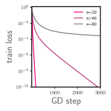
Figure 1: Training loss v.s. number of GD steps for different $n$ in Experiment 1.

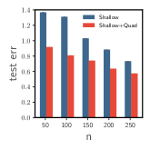
Figure 2: Test error v.s. $n$ in Experiment 2 by the two models with $m=8192$.

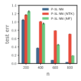
Figure 3: Test error v.s. $n$ in Experiment 3 by the three models with $m=8192$.

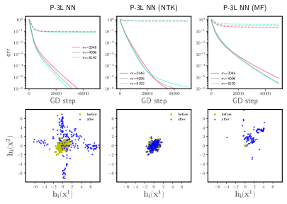
Figure 4: Results of Experiment 3 when $n=600$. Each column corresponds to a different scaling of the P-$3$L NN model, as described in Table 1. Row 1: Evolution of training loss (solid curve) and test error (dashed curve) during training. Row 2: Distribution of the hidden-layer feature map (pre-activation) associated with two particular input data points. Each dot represents a different $i$, (i.e., neuron in the second hidden layer,) and the $x$- and $y$-coordinates equal $h_{i}(\bm{x}_{1})$ and $h_{i}(\bm{x}_{2})$, respectively, where $\bm{x}_{1}$ is an input from the training set and $\bm{x}_{2}$ is an input from the test set.

5 Conclusions and limitations

We consider a general type of models that includes shallow and partially-trained multi-layer NNs, which exhibits feature learning when trained via GF, and prove non-asymptotic global convergence guarantees that accommodates a general class of activation functions. For a randomly-initialized shallow NN in the MF scaling that is wide enough, we prove that by performing GF on the input-layer weights, the training loss converges to zero at a linear rate if the number of training data does not exceed the input dimension. For a randomly-initialized multi-layer NN with large widths, we prove that by performing GF on the weights in the second-to-last layer, the same result holds except there is no requirement on the input dimension. We also perform numerical experiments to demonstrate the advantage of feature learning in our partially-trained multi-layer NNs relative to their counterparts under the NTK scaling.

Our work focuses on the optimization rather than the approximation or generalization properties of NNs, which are also crucial to understand. In addition, as our current theoretical results on global convergence neglect the bias terms and assume that the last-layer weights are untrained, a more general version is left for future work.

Appendix A Additional notations

• For a positive integer $n$, we let $[n]$ denote the set $\{1,...,n\}$.

• We use $i,j$ (as subscripts) to index the neurons in the hidden layers, $a,b$ (as subscripts or superscripts) to index different training data points, $t$ (as a superscript) to denote the training time / time parameter in gradient flow.

• We write $\overline{\sum_{a}}$ for $\frac{1}{n}\sum_{a=1}^{n}$.

• We use bold letters (e.g. $\bm{x}$, $\bm{z}$, $\bm{c}$, $\bm{y}$) to denote vectors.

• We use $W$ and $\{W_{ij}\}_{i\in[m],j\in[D]}$ interchangeably to refer to the same set of parameters.

Appendix B Consistency of the scaling and GD update rule with Xavier initialization

Consider a three-layer network defined by

$$f(\bm{x})= \sum_{i=1}^{m}\theta^{(3)}_{i}\sigma\big{(}{h}_{i}(\bm{x})\big{)}$$ (25)

$$\forall i\in[m]\quad:\quad{h}_{i}(\bm{x})= \sum_{j=1}^{m}\theta^{(2)}_{ij}\sigma\Big{(}\frac{1}{\sqrt{d}}\sum_{k=1}^{d}\theta^{(1)}_{jk}x_{k}\Big{)}$$ (26)

with weight parameters $\big{\{}\theta^{(1)}_{jk}\big{\}}_{j,k\in[m]}$, $\big{\{}\theta^{(2)}_{ij}\big{\}}_{i,j\in[m]}$ and $\big{\{}\theta^{(3)}_{i}\big{\}}_{i\in[m]}$ are initialized according to Xavier initialization, which means that we sample each $\theta^{(1)}_{jk}$ i.i.d. from $\mathcal{N}(0,\frac{1}{m+d})$, each $\theta^{(2)}_{ij}$ i.i.d. from $\mathcal{N}(0,\frac{1}{2m})$, and each $\theta^{(3)}_{i}$ i.i.d. from $\mathcal{N}(0,\frac{1}{m+1})$. If $m\gg d$, both $\mathcal{N}(0,\frac{1}{m+d})$ and $\mathcal{N}(0,\frac{1}{m+1})$ can be approximated by $\mathcal{N}(0,\frac{1}{m})$. Then, up to this approximation, by redefining $c_{i}=\sqrt{m}\theta^{(3)}_{i}$, $W_{ij}=\sqrt{m}\theta^{(2)}_{ij}$ and $z_{jk}=\sqrt{m}\theta^{(1)}_{jk}$, we can write

$$f(\bm{x})= \frac{1}{\sqrt{m}}\sum_{i=1}^{m}c_{i}\sigma\big{(}h_{i}(\bm{x})\big{)}~{},$$ (27)

$$\forall i\in[m]\quad:\quad h_{i}(\bm{x})= \frac{1}{\sqrt{m}}\sum_{j=1}^{D}W_{ij}\sigma\Big{(}\frac{1}{\sqrt{md}}\bm{z}_{j}^{\intercal}\bm{x}\Big{)}~{},$$ (28)

and note that $c_{i},W_{ij}$ and $z_{jk}$ are all initialized i.i.d. of order $O(1)$. In addition, if $\sigma$ is homogeneous, this is then equivalent to (4) and (5) when $D=m$.

Moreover, there is $\frac{\partial f}{\partial W_{ij}}(\bm{x})=\frac{1}{\sqrt{m}}\frac{\partial f}{\partial\theta^{(2)}_{ij}}(\bm{x})$. Then, since performing GD on $\theta^{(2)}_{ij}$ with step size $\delta$ means updating $\theta^{(2)}_{ij}$ according to

$$\theta^{(2)}_{ij}\leftarrow\theta^{(2)}_{ij}-\delta\frac{\partial\mathcal{L}[f]}{\partial\theta^{(2)}_{ij}}~{},$$ (29)

this is equivalent to updating $W_{ij}$ according to

$$\begin{split}W_{ij}\leftarrow&\sqrt{m}\big{(}\theta^{(2)}_{ij}-\delta\frac{\partial\mathcal{L}[f]}{\partial\theta^{(2)}_{ij}}\big{)}\\ =&W_{ij}-m\delta\frac{\partial\mathcal{L}[f]}{\partial W_{ij}}(\bm{x})~{},\end{split}$$ (30)

which justifies the $m$ factor on the right-hand-side of (9).

Appendix C Relationship to the maximum-update parameterization and feature learning

Consider the partially-trained $L$-layer NN model defined in Section H in the case where $D=m\gg d$. In the framework of abc-parameterization introduced in [73], our model corresponds to setting

$$a_{1}=0,\ a_{2}=...= a_{L}=\frac{1}{2},\ a_{L+1}=1$$

$$b_{l}= 0,\ \forall l\in[L+1]$$

Furthermore, as we explain in Appendix B, the appropriate learning rate scales linearly with $m$ (as in (9)), which corresponds to having

$$c=-1$$ (31)

Meanwhile, the maximum-update ($\mu$P) parameterization [73] is characterized by setting

$$a_{1}=-\frac{1}{2},\ a_{2}=...= a_{L}=0,\ a_{L+1}=\frac{1}{2}$$ (32)

$$b_{l}= \frac{1}{2},\ \forall l\in[L+1]$$ (33)

$$c= 0$$ (34)

Recall the symmetry of abc-parameterization derived in [73], which states that one gets a different but equivalent abc-parameterization by setting

$$a_{l}\leftarrow a_{l}+\theta,\ b_{l}\leftarrow b_{l}-\theta,\ c\leftarrow c-2\theta$$ (35)

Since our parameterization can be obtained from the maximum-update parameterization by applying the transformation above with $\theta=\frac{1}{2}$, they are equivalent in the function space. In particular, for our parameterization, the $r$ parameter defined in [73] can be computed as

$$\begin{split}r=&\min\{b_{L+1},a_{L+1}+c\}+a_{L+1}+c+\min_{l=1,...,L}\{2a_{l}-\mathds{1}_{l\neq 1}\}\\ =&\min\{0,1+(-1)\}+1+(-1)+\min\{2\cdot 0-0,2\cdot\frac{1}{2}-1\}\\ =&0\end{split}$$ (36)

Hence, according to [73], our parameterization exhibits feature learning.

Appendix D Proof of Lemma 1

Since we assume that $G$ is positive definite and $|c_{i}|=\hat{c}>0$, $\forall i\in[m]$, we can derive from (14) that

$$\begin{split}\dot{\mathcal{L}}^{t}=&-\frac{\hat{c}^{2}}{m}\sum_{i=1}^{m}\sum_{a,b=1}^{n}\left(f^{t}(\bm{x}_{a})-y_{a}\right)\left(f^{t}(\bm{x}_{b})-y_{b}\right)\sigma^{\prime}\big{(}h_{i}^{t}(\bm{x}_{a})\big{)}\sigma^{\prime}\big{(}h_{i}^{t}(\bm{x}_{a})\big{)}G_{ab}\\ \leq&-\hat{c}^{2}\lambda_{\min}\big{(}G\big{)}\frac{1}{m}\sum_{i=1}^{m}\sum_{a=1}^{n}\left(f^{t}(\bm{x}_{a})-y_{a}\right)^{2}\left(\sigma^{\prime}\big{(}h_{i}(\bm{x}_{a})\big{)}\right)^{2}\\ =&-\hat{c}^{2}\lambda_{\min}\big{(}G\big{)}\sum_{a=1}^{n}\left(f^{t}(\bm{x}_{a})-y_{a}\right)^{2}\frac{1}{m}\sum_{i=1}^{m}\left(\sigma^{\prime}\big{(}h_{i}(\bm{x}_{a})\big{)}\right)^{2}\\ \leq&-\hat{c}^{2}\lambda_{\min}(G)\sum_{a=1}^{n}\left(f^{t}(\bm{x}_{a})-y_{a}\right)^{2}\frac{1}{m}\sum_{i=1}^{m}\mathds{1}_{h_{i}^{t}(\bm{x}_{a})\in I}\left(K_{\sigma^{\prime}}\right)^{2}\\ \leq&-\hat{c}^{2}\lambda_{\min}(G)\left(K_{\sigma^{\prime}}\right)^{2}\sum_{a=1}^{n}\left(f^{t}(\bm{x}_{a})-y_{a}\right)^{2}\min_{b\in[n]}\left\{\frac{1}{m}\sum_{i=1}^{m}\mathds{1}_{h_{i}^{t}(\bm{x}_{b})\in I}\right\}\\ \leq&-{2\hat{c}^{2}\lambda_{\min}(G)\left(K_{\sigma^{\prime}}\right)^{2}}\mathcal{L}^{t}\min_{a\in[n]}\left\{\frac{1}{m}\sum_{i=1}^{m}\mathds{1}_{h_{i}^{t}(\bm{x}_{a})\in I}\right\}\end{split}$$ (37)

Since $I$ is an open interval, $\exists\xi>0$ such that we can find a subinterval $I_{0}\subseteq I$ such that the distance between $I_{0}$ and the boundaries of $I$ (if $I$ is bounded on either side) is no less than $\xi$, i.e.,

$$\inf_{u\in I_{0},u^{\prime}\in\mathbb{R}\setminus I}|u-u^{\prime}|\geq\xi$$ (38)

In particular, we can choose $\xi=\frac{1}{3}(I_{r}-I_{l})$ and $I_{0}=(I_{l}+\xi,I_{r}-\xi)$. Then there is

$$\begin{split}\mathds{1}_{h_{i}^{t}(\bm{x}_{a})\in I}\geq&\mathds{1}_{h_{i}^{0}(\bm{x}_{a})\in I_{0}~{},~{}h_{i}^{t}(\bm{x}_{a})\in I}\\ \geq&\mathds{1}_{h_{i}^{0}(\bm{x}_{a})\in I_{0}~{},~{}|h_{i}^{t}(\bm{x}_{a})-h_{i}^{0}(\bm{x}_{a})|<\xi}\\ \geq&\mathds{1}_{h_{i}^{0}(\bm{x}_{a})\in I_{0}}-\mathds{1}_{|h_{i}^{t}(\bm{x}_{a})-h_{i}^{0}(\bm{x}_{a})|\geq\xi}\end{split}$$ (39)

and so

$$\min_{a\in[n]}\left\{\frac{1}{m}\sum_{i=1}^{m}\mathds{1}_{h_{i}^{t}(\bm{x}_{a})\in I}\right\}\geq\min_{a\in[n]}\left\{\frac{1}{m}\sum_{i=1}^{m}\mathds{1}_{h_{i}^{0}(\bm{x}_{a})\in I_{0}}\right\}-\max_{a\in[n]}\left\{\frac{1}{m}\sum_{i=1}^{m}\mathds{1}_{|h_{i}^{t}(\bm{x}_{a})-h_{i}^{0}(\bm{x}_{a})|\geq\xi}\right\}$$ (40)

Thus, we have

$$\dot{\mathcal{L}}^{t}\leq-2\hat{c}^{2}\lambda_{\min}(G)\left(K_{\sigma^{\prime}}\right)^{2}\mathcal{L}^{t}\left(\min_{a\in[n]}\left\{\frac{1}{m}\sum_{i=1}^{m}\mathds{1}_{h_{i}^{0}(\bm{x}_{a})\in I_{0}}\right\}-\max_{a\in[n]}\left\{\frac{1}{m}\sum_{i=1}^{m}\mathds{1}_{|h_{i}^{t}(\bm{x}_{a})-h_{i}^{0}(\bm{x}_{a})|\geq\xi}\right\}\right)$$ (41)

Meanwhile, since

$$\dot{h}_{i}^{t}(\bm{x}_{a})=-{c_{i}}\sum_{b=1}^{n}\left(f^{t}(\bm{x}_{b})-y_{b}\right)\sigma^{\prime}\big{(}h_{i}^{t}(\bm{x}_{b})\big{)}G_{ab}~{},$$ (42)

there is

$$\begin{split}\frac{1}{m}\sum_{i=1}^{m}\left|\dot{h}_{i}^{t}(\bm{x}_{a})\right|\leq&\hat{c}\frac{1}{m}\sum_{i=1}^{m}\left|\sum_{b=1}^{n}\left(f^{t}(\bm{x}_{b})-y_{b}\right)\sigma^{\prime}\big{(}h_{i}^{t}(\bm{x}_{b})\big{)}G_{ab}\right|\\ \leq&\hat{c}\left(\frac{1}{m}\sum_{i=1}^{m}\left|\sum_{b=1}^{n}\left(f^{t}(\bm{x}_{b})-y_{b}\right)\sigma^{\prime}\big{(}h_{i}^{t}(\bm{x}_{b})\big{)}G_{ab}\right|^{2}\right)^{\frac{1}{2}}\\ \leq&\hat{c}\left(\frac{1}{m}\sum_{i=1}^{m}\sum_{b=1}^{n}\left|\left(f^{t}(\bm{x}_{b})-y_{b}\right)\sigma^{\prime}\big{(}h_{i}^{t}(\bm{x}_{b})\big{)}G_{ab}\right|^{2}\right)^{\frac{1}{2}}\\ \leq&\hat{c}\lambda_{\max}(G)\left(\frac{1}{m}\sum_{i=1}^{m}\sum_{b=1}^{n}\left(f^{t}(\bm{x}_{b})-y_{b}\right)^{2}\left(\sigma^{\prime}\big{(}h_{i}^{t}(\bm{x}_{b})\big{)}\right)^{2}\right)^{\frac{1}{2}}\\ \leq&\hat{c}\lambda_{\max}(G)\left(\frac{\left|\dot{\mathcal{L}}^{t}\right|}{(\hat{c})^{2}\lambda_{\min}\left(G\right)}\right)^{\frac{1}{2}}\\ \leq&\lambda_{\max}(G)\left(\lambda_{\min}\left(G\right)\right)^{-\frac{1}{2}}\left|\dot{\mathcal{L}}^{t}\right|^{\frac{1}{2}}\end{split}$$ (43)

Therefore,

$$\begin{split}\frac{1}{m}\sum_{i=1}^{m}\left|h_{i}^{t}(\bm{x}_{a})-h_{i}^{0}(\bm{x}_{a})\right|\leq&\int_{0}^{t}\frac{1}{m}\sum_{i=1}^{m}\left|\dot{h}_{i}^{s}(\bm{x}_{a})\right|ds\\ \leq&\lambda_{\max}(G)\left(\lambda_{\min}\left(G\right)\right)^{-\frac{1}{2}}\int_{0}^{t}\left|\dot{\mathcal{L}}^{s}\right|^{\frac{1}{2}}ds\end{split}$$ (44)

Since $\forall\xi\in\mathbb{R}$, there is

$$\xi\cdot\mathds{1}_{|h_{i}^{t}(\bm{x}_{a})-h_{i}^{0}(\bm{x}_{a})|\geq\xi}\leq\left|h_{i}^{t}(\bm{x}_{a})-h_{i}^{0}(\bm{x}_{a})\right|~{},$$ (45)

we derive that, $\forall a\in[n]$,

$$\begin{split}\frac{1}{m}\sum_{i=1}^{m}\mathds{1}_{|h_{i}^{t}(\bm{x}_{a})-h_{i}^{0}(\bm{x}_{a})|\geq\xi}\leq&\xi^{-1}\frac{1}{m}\sum_{i=1}^{m}\left|h_{i}^{t}(\bm{x}_{a})-h_{i}^{0}(\bm{x}_{a})\right|\\ \leq&C_{1}\int_{0}^{t}\left|\dot{\mathcal{L}}^{s}\right|^{\frac{1}{2}}ds~{},\end{split}$$ (46)

where we set $C_{1}=\lambda_{\max}(G)\left(\lambda_{\min}\left(G\right)\right)^{-\frac{1}{2}}\xi^{-1}>0$ for simplicity. As a consequence,

$$\max_{a\in[n]}\left\{\frac{1}{m}\sum_{i=1}^{m}\mathds{1}_{|h_{i}^{t}(\bm{x}_{a})-h_{i}^{0}(\bm{x}_{a})|\geq\xi}\right\}\leq C_{1}\int_{0}^{t}\left|\dot{\mathcal{L}}^{s}\right|^{\frac{1}{2}}ds$$ (47)

Define

$$\tilde{\eta}^{t}=\min_{a\in[n]}\left\{\frac{1}{m}\sum_{i=1}^{m}\mathds{1}_{h_{i}^{0}(\bm{x}_{a})\in I_{0}}\right\}-C_{1}\int_{0}^{t}\left|\dot{\mathcal{L}}^{s}\right|^{\frac{1}{2}}ds$$ (48)

Note that at $t=0$, there is $\tilde{\eta}^{t}=\min_{a\in[n]}\left\{\frac{1}{m}\sum_{i=1}^{m}\mathds{1}_{h_{i}^{0}(\bm{x}_{a})\in I_{0}}\right\}$. Then, on one hand, we know from (40) and (47) that $\forall t\geq 0$,

$$\eta^{t}\geq\min_{a\in[n]}\left\{\frac{1}{m}\sum_{i=1}^{m}\mathds{1}_{h_{i}^{0}(\bm{x}_{a})\in I_{0}}\right\}-\max_{a\in[n]}\left\{\frac{1}{m}\sum_{i=1}^{m}\mathds{1}_{|h_{i}^{t}(\bm{x}_{a})-h_{i}^{0}(\bm{x}_{a})|\geq\xi}\right\}\geq\tilde{\eta}^{t}~{},$$ (49)

Hence, (41) implies that

$$\begin{split}\dot{\mathcal{L}}^{t}\leq&-2\hat{c}^{2}\lambda_{\min}(G)\left(K_{\sigma^{\prime}}\right)^{2}\mathcal{L}^{t}\eta^{t}\\ \leq&-2\hat{c}^{2}\lambda_{\min}(G)\left(K_{\sigma^{\prime}}\right)^{2}\mathcal{L}^{t}\tilde{\eta}^{t}\end{split}$$ (50)

On the other hand, by the definition of $\tilde{\eta}^{t}$,

$$\begin{split}\dot{\tilde{\eta}}^{t}=&-C_{1}\left|\dot{\mathcal{L}}^{t}\right|^{\frac{1}{2}}\\ \geq&-C_{1}\left|\dot{\mathcal{L}}^{t}\right|\cdot\left|\dot{\mathcal{L}}^{t}\right|^{-\frac{1}{2}}\\ \geq&C_{1}\dot{\mathcal{L}}^{t}\left(2\hat{c}^{2}\lambda_{\min}(G)\left(K_{\sigma^{\prime}}\right)^{2}\mathcal{L}^{t}\tilde{\eta}^{t}\right)^{-\frac{1}{2}}\\ \geq&C_{2}(\hat{c})^{-1}\dot{\mathcal{L}}^{t}\left(\mathcal{L}^{t}\right)^{-\frac{1}{2}}\left(\tilde{\eta}^{t}\right)^{-\frac{1}{2}}~{},\end{split}$$ (51)

where we set $C_{2}=2^{-\frac{1}{2}}C_{1}\left(\lambda_{\min}(G)\right)^{-\frac{1}{2}}(K_{\sigma^{\prime}})^{-1}=\frac{\lambda_{\max}(G)}{\sqrt{2}\xi K_{\sigma^{\prime}}\lambda_{\min}(G)}\leq\frac{nG_{\max}}{\sqrt{2}\xi K_{\sigma^{\prime}}\lambda_{\min}(G)}$ for simplicity. Therefore, when $\eta^{t}>0$,

$$\begin{split}\frac{d}{dt}\left(\frac{2}{3}\left(\tilde{\eta}^{t}\right)^{\frac{3}{2}}\right)=\left(\tilde{\eta}^{t}\right)^{\frac{1}{2}}\dot{\tilde{\eta}}^{t}\geq C_{2}(\hat{c})^{-1}\dot{\mathcal{L}}^{t}\left(\mathcal{L}^{t}\right)^{-\frac{1}{2}}\geq C_{2}(\hat{c})^{-1}\frac{d}{dt}\left(2\mathcal{L}^{t}\right)^{\frac{1}{2}}~{},\end{split}$$ (52)

which implies that

$$\frac{2}{3}\left(\tilde{\eta}^{t}\right)^{\frac{3}{2}}-\frac{2}{3}\left(\tilde{\eta}^{0}\right)^{\frac{3}{2}}\geq C_{2}(\hat{c})^{-1}\left(\left(2\mathcal{L}^{t}\right)^{\frac{1}{2}}-\left(2\mathcal{L}^{0}\right)^{\frac{1}{2}}\right)\geq-C_{2}(\hat{c})^{-1}\left(2\mathcal{L}^{0}\right)^{\frac{1}{2}}$$ (53)

and so $\forall t\geq 0$,

$$\frac{2}{3}\left(\eta^{t}\right)^{\frac{3}{2}}\geq\frac{2}{3}\left(\tilde{\eta}^{t}\right)^{\frac{3}{2}}\geq\frac{2}{3}\left(\tilde{\eta}^{0}\right)^{\frac{3}{2}}-C_{2}(\hat{c})^{-1}\left(2\mathcal{L}^{0}\right)^{\frac{1}{2}}$$ (54)

Appendix E Proof of Theorem 1

To apply Lemma 1, we need two additional lemmas, which we will prove in Appendix E.1 and E.2. The first one guarantees that the loss value at initialization, $\mathcal{L}^{0}$, is upper-bounded with high probability:

Lemma 2.

$\forall\delta>0$, if $m\geq\Omega\left(\hat{c}^{2}\log\left(n\delta^{-1}\right)G_{\max}/\|\bm{y}\|^{2}\right)$, then with probability at least $1-\delta$, there is

$$\mathcal{L}^{0}\leq\|\bm{y}\|^{2}$$ (55)

The second one proves that $\tilde{\eta}^{0}$ is lower-bounded with high probability, which heuristically says that there is indeed a nontrivial proportion of neurons in the central part of the active region of $\sigma$, for every $a\in[n]$:

Lemma 3.

$\forall\delta>0$, if $m\geq\frac{\log(n{\delta}^{-1})}{2\left(K(I,G_{\min},G_{\max})\right)^{2}}$, then with probability at least $1-\delta$, there is

$$\eta^{0}>K(I,G_{\min},G_{\max})~{},$$ (56)

where $K(I,\lambda_{1},\lambda_{2})=\frac{1}{6\sqrt{2\pi}\lambda_{2}}(I_{r}-I_{l})\exp\left\{-\frac{\max\{|I_{l}|,|I_{r}|\}}{(\lambda_{1})^{2}}\right\}$ is a positive number that depends on $I$, $\lambda_{1}$ and $\lambda_{2}$.

With these two lemmas, we deduce that $\forall\delta>0$, if $m\geq\Omega\left((1+\hat{c}^{2}/\|\bm{y}\|^{2})\log\left(n\delta^{-1}\right)\right)$, then with probability at least $\delta$, there is $\forall t\geq 0$,

$$\frac{2}{3}\left(\eta^{t}\right)^{\frac{3}{2}}\geq\frac{2}{3}\left(K(I,G_{\min},G_{\max})\right)^{\frac{3}{2}}-\sqrt{2}C_{2}(\hat{c})^{-1}\|\bm{y}\|~{},$$ (57)

where $K(I,G_{\min},G_{\max})$ is defined as in Lemma 3. Therefore, if our choice of $\hat{c}$ satisfies

$$\hat{c}\geq\frac{3\sqrt{2}C_{2}\|\bm{y}\|}{\left(K(I,G_{\min},G_{\max})\right)^{\frac{3}{2}}}~{},$$ (58)

then there is $\forall t\geq 0$,

$$\eta^{t}\geq 2^{-\frac{2}{3}}K(I,G_{\min},G_{\max})>0~{},$$ (59)

in which case (50) gives

$$\dot{\mathcal{L}}^{t}\leq-2^{\frac{1}{3}}\hat{c}^{2}\lambda_{\min}(G)\left(K_{\sigma^{\prime}}\right)^{2}\mathcal{L}^{t}K(I,G_{\min},G_{\max})~{},$$ (60)

which will allow us to finally conclude that

$$\mathcal{L}^{t}\leq\mathcal{L}^{0}\exp\left\{-2^{\frac{1}{3}}\lambda_{\min}(G)\left(K_{\sigma^{\prime}}\right)^{2}K(I,G_{\min},G_{\max})\hat{c}^{2}t\right\}$$ (61)

Note that (60) establishes a PL condition. Several other convergence analyses of NNs have also relied on variants of the PL condition [25, 44, 74].

E.1 Proof of Lemma 2

Proof.

Since at initialization, $\big{\{}c_{i}\big{\}}_{i\in[m]}$ and $\big{\{}W_{ij}^{0}\big{\}}_{i\in[m],j\in[D]}$ are both sampled i.i.d. and $\big{\{}c_{i}\big{\}}_{i\in[m]}$ has mean zero, we know that $\forall a\in[n]$, $f^{0}(\bm{x}_{a})=\frac{1}{m}\sum_{i=1}^{m}c_{i}\sigma\big{(}h_{i}^{t}(\bm{x}_{a})\big{)}$ is the sample mean of i.i.d. random variables with zero-mean. Moreover, since $\big{\{}W_{ij}^{0}\big{\}}_{i\in[m],j\in[D]}$ is sampled from $\mathcal{N}(0,1)$, we know that $\forall i\in[m]$, the random variable $c_{i}\sigma\big{(}h_{i}^{t}(\bm{x}_{a})\big{)}$ is sub-Gaussian [68], with sub-Gaussian norm

$$\begin{split}\|c_{i}\sigma\big{(}h_{i}^{t}(\bm{x}_{a})\big{)}\|_{\psi_{2}}\leq&\hat{c}\|\sigma\big{(}h_{i}^{t}(\bm{x}_{a})\big{)}\|_{\psi_{2}}\\ \leq&\hat{c}L_{\sigma}(G_{aa})^{\frac{1}{2}}M_{SG}\\ \leq&\hat{c}L_{\sigma}(G_{\max})^{\frac{1}{2}}M_{SG}~{},\end{split}$$ (62)

where $M_{SG}>0$ is some absolute constant. Thus, by Hoeffding’s inequality [68], $\forall a\in[n]$, $\forall r>0$,

$$\begin{split}\mathbb{P}\left(\left|f^{0}(\bm{x}_{a})\right|\geq u\right)=&\mathbb{P}\left(\left|\frac{1}{m}\sum_{i=1}^{m}c_{i}\sigma\big{(}h_{i}^{t}(\bm{x}_{a})\big{)}\right|\geq u\right)\\ \leq&2\exp\left\{-\frac{Ku^{2}m}{\|c_{i}\sigma\big{(}h_{i}^{t}(\bm{x}_{a})\big{)}\|_{\psi_{2}}^{2}}\right\}\\ \leq&2\exp\left\{-\frac{Ku^{2}m}{\hat{c}^{2}(L_{\sigma})^{2}G_{\max}(M_{SG})^{2}}\right\}~{},\end{split}$$ (63)

where $K$ is some absolute constant. Hence, by union bound,

$$\begin{split}\mathbb{P}\left(\sum_{a=1}^{n}\left|f^{0}(\bm{x}_{a})\right|^{2}\geq\|\bm{y}\|^{2}\right)\leq&\sum_{a=1}^{n}\mathbb{P}\left(\left|f^{0}(\bm{x}_{a})\right|\geq\|\bm{y}\|\right)\\ \leq&2n\exp\left\{-\frac{K\|\bm{y}\|^{2}m}{\hat{c}^{2}(L_{\sigma})^{2}G_{\max}(M_{SG})^{2}}\right\}\end{split}$$ (64)

Thus, $\forall\delta>0$, if

$$m\geq\hat{c}^{2}(L_{\sigma})^{2}G_{\max}K^{-1}(M_{SG})^{2}\|\bm{y}\|^{-2}\log\left(\frac{2n}{\delta}\right)$$ (65)

then with probability at least $1-\delta$, there is

$$\begin{split}\mathcal{L}^{0}=&\frac{1}{2}\sum_{a=1}^{n}\left|f^{0}(\bm{x}_{a})-y_{a}\right|^{2}\\ \leq&\frac{1}{2}\sum_{a=1}^{n}\left|f^{0}(\bm{x}_{a})\right|^{2}+\frac{1}{2}\|\bm{y}\|^{2}\\ \leq&\|\bm{y}\|^{2}\end{split}$$ (66)

∎

E.2 Proof of Lemma 3

Since each $W_{ij}^{0}$ are sampled i.i.d. from $\mathcal{N}(0,1)$, we know that $\forall a\in[n]$, independently for each $i\in[m]$, $h_{i}^{0}(\bm{x}_{a})$ follows a Gaussian distribution with mean 0 and variance $G_{aa}$. Therefore,

$$\sum_{i=1}^{m}\mathds{1}_{h_{i}^{0}(\bm{x}^{a})\notin I_{0}}\sim\text{Binomial}\left(m,1-\pi\left(I_{0};G_{aa}\right)\right)~{},$$ (67)

Hence, by Hoeffding’s inequality, $\forall a\in[n]$, $\forall r>0$,

$$\mathbb{P}\left(\frac{1}{m}\sum_{i=1}^{m}\mathds{1}_{h_{i}^{0}(x_{a})\notin I_{0}}\geq 1-\pi(I_{0};G_{aa})+r\right)\leq\exp\left\{-2mr^{2}\right\}$$ (68)

$\forall a\in[n]$, choosing $r=\frac{1}{2}\pi\left(I_{0};G_{aa}\right)$, we then get

$$\begin{split}\mathbb{P}\left(\frac{1}{m}\sum_{i=1}^{m}\mathds{1}_{h_{i}^{0}(x_{a})\in I_{0}}\leq\frac{1}{2}\pi\left(I_{0};G_{aa}\right)\right)=&\mathbb{P}\left(\frac{1}{m}\sum_{i=1}^{m}\mathds{1}_{h_{i}^{0}(x_{a})\notin I_{0}}\geq 1-\frac{1}{2}\pi\left(I_{0};G_{aa}\right)\right)\\ \leq&\exp\left\{-\frac{1}{2}m\left(\pi\left(I_{0};G_{aa}\right)\right)^{2}\right\}\\ \leq&\exp\left\{-\frac{1}{2}m\left(\min_{b\in[n]}\left\{\pi\left(I_{0};G_{bb}\right)\right\}\right)^{2}\right\}\end{split}$$ (69)

and so by union bound

$$\begin{split}\mathbb{P}\left(\tilde{\eta}^{0}\leq\frac{1}{2}\min_{b\in[n]}\left\{\pi\left(I_{0};G_{bb}\right)\right\}\right)=&\mathbb{P}\left(\min_{a\in[n]}\left\{\frac{1}{m}\sum_{i=1}^{m}\mathds{1}_{h_{i}^{0}(x_{a})\in I_{0}}\right\}<\frac{1}{2}\min_{b\in[n]}\left\{\pi\left(I_{0};G_{bb}\right)\right\}\right)\\ \leq&\sum_{a=1}^{n}\mathbb{P}\left(\frac{1}{m}\sum_{i=1}^{m}\mathds{1}_{h_{i}^{0}(x_{a})\in I_{0}}<\frac{1}{2}\min_{b\in[n]}\left\{\pi\left(I_{0};G_{bb}\right)\right\}\right)\\ \leq&\sum_{a=1}^{n}\mathbb{P}\left(\frac{1}{m}\sum_{i=1}^{m}\mathds{1}_{h_{i}^{0}(x_{a})\in I_{0}}<\frac{1}{2}\pi\left(I_{0};G_{aa}\right)\right)\\ \leq&n\exp\left\{-\frac{1}{2}m\left(\min_{b\in[n]}\left\{\pi\left(I_{0};G_{bb}\right)\right\}\right)^{2}\right\}\end{split}$$ (70)

Since $\forall b\in[n]$, there is $G_{\min}\leq G_{bb}\leq G_{\max}$,

$$\begin{split}\pi\left(I_{0};G_{bb}\right)=&\frac{1}{\sqrt{2\pi G_{bb}}}\int_{I_{l}+\xi}^{I_{r}-\xi}e^{-\frac{u^{2}}{G_{bb}}}du\\ \geq&\frac{1}{\sqrt{2\pi G_{bb}}}(I_{r}-I_{l}-2\xi)\inf_{I_{l}+\xi\leq u\leq I_{r}-\xi}\exp\left\{-\frac{u^{2}}{G_{bb}}\right\}\\ \geq&\frac{1}{\sqrt{2\pi G_{\max}}}(I_{r}-I_{l}-2\xi)\exp\left\{-\frac{\max\{|I_{l}|,|I_{r}|\}}{(G_{\min})^{2}}\right\}\\ \geq&\frac{1}{3\sqrt{2\pi}G_{\max}}(I_{r}-I_{l})\exp\left\{-\frac{\max\{|I_{l}|,|I_{r}|\}}{(G_{\min})^{2}}\right\}\end{split}$$ (71)

Letting $K(I,\lambda_{1},\lambda_{2})=\frac{1}{6\sqrt{2\pi}\lambda_{2}}(I_{r}-I_{l})\exp\left\{-\frac{\max\{|I_{l}|,|I_{r}|\}}{(\lambda_{1})^{2}}\right\}>0$, we can then write

$$\begin{split}\mathbb{P}\left(\tilde{\eta}^{0}\leq K(I,G_{\min},G_{\max})\right)\leq&\mathbb{P}\left(\tilde{\eta}_{0}\leq\frac{1}{2}\min_{b\in[n]}\left\{\pi\left(I_{0};G_{bb}\right)\right\}\right)\\ \leq&n\exp\left\{-2m\left(K(I,G_{\min},G_{\max})\right)^{2}\right\}\end{split}$$ (72)

Thus, $\forall\delta>0$, if $m\geq\frac{\log(n{\delta}^{-1})}{2\left(K(I,G_{\min},G_{\max})\right)^{2}}$, then with probability at least $1-\delta$, it holds that $\tilde{\eta}^{0}>K(I,G_{\min},G_{\max})>0$.

Appendix F Proof of Theorem 2

By Condition 1, we know that $\forall\delta>0$, if $D\geq D_{\min}(\frac{1}{2}\delta,\frac{1}{2}\lambda_{\min}(\bar{G}))$, then with probability at least $1-\frac{1}{2}\delta$, there is $\|G-\bar{G}\|_{2}\leq\frac{1}{2}\lambda_{\min}(\bar{G})$, and hence $\lambda_{\min}(G)\geq\frac{1}{2}\lambda_{\min}(\bar{G})$, $G_{\min}\geq\frac{1}{2}\bar{G}_{\min}$, $\lambda_{\max}(G)\leq\lambda_{\max}(\bar{G})+\frac{1}{2}\lambda_{\min}(\bar{G})\leq 2\lambda_{\max}(\bar{G})$, and $G_{\max}\leq 2\bar{G}_{\max}$. We then perform the following analysis conditioned on the event that $\|G-\bar{G}\|_{2}\leq\frac{1}{2}\lambda_{\min}(\bar{G})$.

Since the sampling of $\big{\{}c_{i}\big{\}}_{i\in[m]}$ and $\big{\{}W_{ij}^{0}\big{\}}_{i\in[m],j\in[D]}$ is independent from the realization of $G$, we know from Lemma 3 that if $m\geq\frac{\log(4n{\delta}^{-1})}{2\left(K(I,\frac{1}{2}\lambda_{\min}(\bar{G}),2\lambda_{\max}(\bar{G}))\right)^{2}}\geq\frac{\log(4n{\delta}^{-1})}{2\left(K(I,G_{\min},G_{\max})\right)^{2}}$, then with probability at least $1-\frac{1}{4}\delta$, there is

$$\tilde{\eta}^{0}>K(I,G_{\min},G_{\max})\geq K(I,\frac{1}{2}\bar{G}_{\min},2\bar{G}_{\max})$$ (73)

From Lemma 2, we also know that if $m\geq\Omega\left(\hat{c}^{2}\log\left(n\delta^{-1}\right)\lambda_{\max}(\bar{G})/\|\bm{y}\|^{2}\right)\geq\Omega\left(\hat{c}^{2}\log\left(n\delta^{-1}\right)\lambda_{\max}(G)/\|\bm{y}\|^{2}\right)$, then with probability at least $1-\frac{1}{4}\delta$, there is $\mathcal{L}^{0}\leq\|\bm{y}\|^{2}$. Therefore, in total, we know that with probability at least $1-\delta$, the following conditions all hold:

$$\|G-\bar{G}\|_{2}\leq \frac{1}{2}\lambda_{\min}(\bar{G})~{},$$ (74)

$$\tilde{\eta}^{0}\geq K(I,\frac{1}{2}\bar{G}_{\min},2\bar{G}_{\max})~{},$$ (75)

$$\mathcal{L}^{0}\leq \|\bm{y}\|^{2}~{},$$ (76)

in which case, by applying Lemma 1 with $G=G^{(1)}$, we get

$$\big{(}\eta^{t}\big{)}^{\frac{3}{2}}\geq\big{(}\tilde{\eta}^{0}\big{)}^{\frac{3}{2}}-K_{1}(\lambda_{\min}\left(G\right),\lambda_{\max}\left(G\right))(\hat{c})^{-1}\left(\left(\mathcal{L}^{0}\right)^{\frac{1}{2}}-\left(\mathcal{L}^{t}\right)^{\frac{1}{2}}\right)~{},$$ (77)

where $K_{1}(\lambda_{1},\lambda_{2})=\frac{9}{2}\lambda_{1}^{-1}\lambda_{2}K_{\sigma^{\prime}}^{-1}(I_{r}-I_{l})>0$. Thus, by the definition of $K_{1}(\cdot,\cdot)$, we know that

$$K_{1}(\lambda_{\min}\left(G\right),\lambda_{\max}\left(G\right))\leq 4K_{1}(\lambda_{\min}\left(\bar{G}\right),\lambda_{\max}\left(\bar{G}\right))~{},$$ (78)

and so $\forall t\geq 0$,

$$\begin{split}\big{(}\eta^{t}\big{)}^{\frac{3}{2}}\geq&\big{(}\tilde{\eta}^{0}\big{)}^{\frac{3}{2}}-4K_{1}(\lambda_{\min}\left(\bar{G}\right),\lambda_{\max}\left(\bar{G}\right))(\hat{c})^{-1}\left(\left(\mathcal{L}^{0}\right)^{\frac{1}{2}}-\left(\mathcal{L}^{t}\right)^{\frac{1}{2}}\right)\\ \geq&\big{(}K(I,\frac{1}{2}\bar{G}_{\min},2\bar{G}_{\max})\big{)}^{\frac{3}{2}}-4K_{1}(\lambda_{\min}\left(\bar{G}\right),\lambda_{\max}\left(\bar{G}\right))(\hat{c})^{-1}\|\bm{y}\|\end{split}$$ (79)

Therefore, if our choice of $\hat{c}$ satisfies

$$\hat{c}\geq\frac{8K_{1}(\lambda_{\min}\left(\bar{G}\right),\lambda_{\max}\left(\bar{G}\right))\|\bm{y}\|}{\big{(}K(I,\frac{1}{2}\bar{G}_{\min},2\bar{G}_{\max})\big{)}^{\frac{3}{2}}}$$ (80)

then there is $\forall t\geq 0$,

$$\eta^{t}\geq 2^{-\frac{2}{3}}K(I,\frac{1}{2}\bar{G}_{\min},2\bar{G}_{\max})$$ (81)

Hence, (50) implies that $\forall t\geq 0$,

$$\begin{split}\dot{\mathcal{L}}^{t}\leq&-2\hat{c}^{2}\lambda_{\min}(G)(K_{\sigma^{\prime}})^{2}\mathcal{L}^{t}2^{-\frac{2}{3}}K(I,\frac{1}{2}\bar{G}_{\min},2\bar{G}_{\max})\\ \leq&-2^{-\frac{2}{3}}\hat{c}^{2}\lambda_{\min}(\bar{G})(K_{\sigma^{\prime}})^{2}\mathcal{L}^{t}K(I,\frac{1}{2}\bar{G}_{\min},2\bar{G}_{\max})\end{split}$$ (82)

and therefore

$$\mathcal{L}^{t}\leq\mathcal{L}^{0}\exp\left\{-2^{-\frac{2}{3}}\hat{c}^{2}\lambda_{\min}(\bar{G})(K_{\sigma^{\prime}})^{2}K(I,\frac{1}{2}\bar{G}_{\min},2\bar{G}_{\max})\right\}$$ (83)

Appendix G Proof of Theorem 3

In view of Theorem 2, it is sufficient to verify that Condition 1 holds for $D_{\min}(\delta,u)=\Omega\left(n^{2}u^{-2}\log(n\delta^{-1})\right)$, which is given by the following lemma:

Lemma 4.

$\forall\delta\geq 0$, if $D\geq\Omega\left(n^{2}u^{-2}\log(n\delta^{-1})\right)$ , then with probability at least $1-\delta$,

$$\|G^{(1)}-\bar{G}^{(1)}\|_{2}\leq u$$ (84)

G.1 Proof of Lemma 4

Let $Z$ be a random vector on $\mathbb{R}^{d}$ with law given by $\pi_{\bm{z}}$, and then we can write $\bar{G}^{(1)}_{ab}=\mathbb{E}\left[\sigma(\bm{x}_{a}^{\intercal}Z)\sigma(\bm{x}_{b}^{\intercal}Z)\right]$ for $a,b\in[n]$. By assumption, $Z$ is sub-gaussian with sub-gaussian norm

$$\|Z\|_{\psi_{2}}:=\sup_{x\in S^{d-1}}\|x^{\intercal}Z\|_{\psi_{2}}<\infty$$ (85)

Thus, $\forall a\in[n]$, we have

$$\|\sigma(x_{a}^{\intercal}Z)\|_{\psi_{2}}\leq L_{\sigma}\|x^{\intercal}Z\|_{\psi_{2}}\leq L_{\sigma}\|Z\|_{\psi_{2}}$$ (86)

Hence, by Lemma 2.7.7 in [68], we know that $\forall a,b\in[n]$, $\sigma(x_{a}^{\intercal}Z)\sigma(x_{b}^{\intercal}Z)$ is a sub-exponential random variable with sub-exponential norm

$$\|\sigma(x_{a}^{\intercal}Z)\sigma(x_{b}^{\intercal}Z)\|_{\psi_{1}}\leq\|\sigma(x_{a}^{\intercal}Z)\|_{\psi_{2}}\|\sigma(x_{b}^{\intercal}Z)\|_{\psi_{2}}\leq(L_{\sigma})^{2}\|Z\|_{\psi_{2}}^{2}$$ (87)

Then, by Bernstein’s inequality (Theorem 2.8.1 in [68]), since each $\bm{z}_{j}$ is sampled i.i.d. from $\pi_{\bm{z}}$, we have that $\forall a,b\in[n]$ and $\forall u>0$,

$$\begin{split}\mathbb{P}\left(\left|G^{(1)}_{ab}-\bar{G}^{(1)}_{ab}\right|\geq u\right)=&\mathbb{P}\left(\left|\frac{1}{D}\sum_{j=1}^{D}\sigma(x_{a}^{\intercal}z^{j})\sigma(x_{b}^{\intercal}z^{j})-\mathbb{E}\left[\sigma(x_{a}^{\intercal}Z)\sigma(x_{b}^{\intercal}Z)\right]\right|\geq u\right)\\ \leq&2\exp\left\{-K\min\left\{\frac{u^{2}D}{\|\sigma(x_{a}^{\intercal}Z)\sigma(x_{b}^{\intercal}Z)\|_{\psi_{1}}^{2}},\frac{uD}{\|\sigma(x_{a}^{\intercal}Z)\sigma(x_{b}^{\intercal}Z)\|_{\psi_{1}}}\right\}\right\}\\ \leq&2\exp\left\{-K\min\left\{\frac{u^{2}D}{(L_{\sigma})^{4}\|Z\|_{\psi_{2}}^{4}},\frac{uD}{(L_{\sigma})^{2}\|Z\|_{\psi_{2}}^{2}}\right\}\right\}~{},\end{split}$$ (88)

where $K>0$ is some absolute constant. In other words, for any $\delta^{\prime}>0$, if

$$D\geq\max\left\{\frac{(L_{\sigma})^{4}\|Z\|_{\psi_{2}}^{4}\log(2(\delta^{\prime})^{-1})}{u^{2}K},\frac{(L_{\sigma})^{2}\|Z\|_{\psi_{2}}^{2}\log(2(\delta^{\prime})^{-1})}{uK}\right\}~{},$$ (89)

then we have $\left|G^{(1)}_{ab}-\bar{G}^{(1)}_{ab}\right|\geq u$ with probability at least $1-\delta$. If we choose $u=\frac{u^{\prime}}{n}$ and $\delta^{\prime}=\frac{\delta}{n^{2}}$, then we get, if

$$D\geq\max\left\{\frac{n^{2}(L_{\sigma})^{4}\|Z\|_{\psi_{2}}^{4}\log(2n^{2}\delta^{-1})}{K(u^{\prime})^{2}},\frac{n(L_{\sigma})^{2}\|Z\|_{\psi_{2}}^{2}\log(2n^{2}\delta^{-1})}{Ku^{\prime}}\right\}~{},$$ (90)

then

$$\begin{split}\mathbb{P}\left(\|G^{(1)}-\bar{G}^{(1)}\|_{F}^{2}\geq\left(u^{\prime}\right)^{2}\right)\leq&\sum_{a,b=1}^{n}\mathbb{P}\left(\left|G^{(1)}_{ab}-\bar{G}^{(1)}_{ab}\right|\geq\frac{u^{\prime}}{n}\right)\\ \leq&n^{2}\frac{\delta}{n^{2}}\\ \leq&\delta\end{split}$$ (91)

Hence, with probability at least $1-\delta$, we have

$$\|G^{(1)}-\bar{G}^{(1)}\|_{2}^{2}\leq\|G^{(1)}-\bar{G}^{(1)}\|_{\mathtt{F}}^{2}\leq\left(u^{\prime}\right)^{2}~{},$$ (92)

Appendix H Generalization to deeper models

By setting $\Phi$ to be the activations of the second-to-last hidden-layer of a multi-layer NN, we can obtain generalizations of the P-$3$L NN to deeper architectures. For example, in the feed-forward case, we can obtain the following partially-trained $L$-layer NN:

$$f(\bm{x})=\frac{1}{m}\sum_{i=1}^{m}c_{i}\sigma\big{(}h_{i}^{(L-1)}(\bm{x})\big{)}~{},$$

$$\forall i\in[m]\quad: h_{i}^{(L-1)}(\bm{x})= \frac{1}{\sqrt{D}}\sum_{j=1}^{D}W_{ij}\sigma\big{(}h_{j}^{(L-2)}(\bm{x})\big{)}~{},\qquad$$

$$\forall l\in[L-3],\forall i\in[D]\quad: h_{i}^{(l+1)}(\bm{x})= \frac{1}{\sqrt{D}}\sum_{j=1}^{D}\bar{W}^{(l)}_{ij}\sigma\big{(}h_{j}^{(l)}(\bm{x})\big{)}~{},\qquad$$

$$\forall j\in[D]\quad: h_{j}^{(1)}(\bm{x})= \frac{1}{\sqrt{d}}\bm{z}_{j}^{\intercal}\bm{x}~{},\qquad$$

where $\bar{W}^{(1)},...,\bar{W}^{(L-3)}\in\mathbb{R}^{D\times D}$ and $\bm{z}_{1},...,\bm{z}_{D}\in\mathbb{R}^{d}$ are sampled randomly and fixed. This model can be written in the form of (4) and (5) with $\phi_{j}(\bm{x})=\sigma\big{(}h_{j}^{(L-2)}(\bm{x})\big{)}$. The corresponding Gram matrix is recursively defined and also appears in the NTK analysis [18]. In particular, the results in [18] imply that if $\sigma$ is analytic and not a polynomial, then Condition 1 holds, and hence similar global convergence results can be obtained as corollaries of Theorem 2.

Appendix I Further details of the numerical experiments

In our models, $\big{\{}c_{i}\big{\}}_{i\in[m]}$ is sampled i.i.d. from the Rademacher distribution $\mu_{c}=\frac{1}{2}\bm{\delta}_{1}+\frac{1}{2}\bm{\delta}_{-1}$, $\big{\{}\bm{z}_{j}\big{\}}_{j\in[D]}$ is sampled i.i.d. from $\mathcal{N}(0,I_{d})$, and $\big{\{}W_{ij}\big{\}}_{i\in[m],j\in[D]}$ is initialized by sampling i.i.d. from $\mathcal{N}(0,1)$. In the model under NTK scaling, we additionally symmetrize the model at initialization according to the strategy used in [16] to ensure that the function value at initialization does not blow up when the width is large. We choose to train the models using $50000$ steps of (full-batch) GD with step size $\delta=1$. When the test error is computed, we use a test set of size $500$ generated by sampling i.i.d. from the same distribution as the training set.

The experiments are run with NVIDIA GPUs (1080ti and Titan RTX).

I.1 Experiment $1$

We choose $\sigma$ to be $\tanh$. For each choice of $n$, we run the experiment with $5$ different random seeds, and Figure 3 plots the evolution of the training loss during GD averaged over the $5$ runs with $m=8192$.

Figure 5 is the same as Figure 3 except for having $m=4096$. We see that the two two plots agree well.

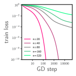
Figure 5: Training loss v.s. number of GD steps for different $n$ in Experiment 1 with $m=4096$.

I.2 Experiment $2$

We choose $\sigma$ to be ReLU. For each choice of $n$ and each of the two models, we experiment with $5$ different random seeds, and Figure 3 plots the test error at the $50000$ GD step averaged over the $5$ runs $\pm$ its standard deviation.

In Figure 6, we plot the evolution of the training loss and test error during GD for the two different models, with $m=2048$ or $8192$ and different choices of $n$, averaged over $5$ runs with different random seeds. We see in particular that the difference between the two choices of $m$ is negligible, suggesting that it is unlikely to obtain performance improvements with further over-parameterization.

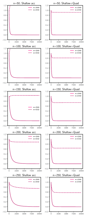
Figure 6: Test error v.s. GD steps in Experiment 2 for the two models and difference choices of $n$.

I.3 Experiment $3$

We choose $\sigma$ to be ReLU and input dimension $d=50$. We use a training set of size $n=600$ for the results reported in Figure 4. The data set is inspired by [69]: We sample both the training and the test set i.i.d. from the distribution $(\bm{x},y)\sim\mathcal{D}$ on $\mathbb{R}^{d+1}$, under which the joint distribution of $(x_{1},x_{2},y)$ is

$$\mathbb{P}(x_{1}=1,x_{2}=0,y=1)= \frac{1}{4}$$ (93)

$$\mathbb{P}(x_{1}=-1,x_{2}=0,y=1)= \frac{1}{4}$$ (94)

$$\mathbb{P}(x_{1}=0,x_{2}=1,y=-1)= \frac{1}{4}$$ (95)

$$\mathbb{P}(x_{1}=0,x_{2}=-1,y=-1)= \frac{1}{4}$$ (96)

and $x_{3},...,x_{d}$ each follow the uniform distribution in $[-1,1]$, independently from each other as well as $x_{1},x_{2}$ and $y$.

Figures 8 and 8 are the same as Figure 4 except for having $n=400$ and $800$, respectively. We see that as $n$ increases, test error improves for all three models, while our P-$3$L NN model remains the one achieving the lowest test error.

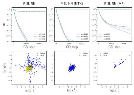
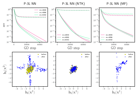
Figure 7: Same as Figure 4 except for setting $n=400$.

Figure 8: Same as Figure 4 except for setting $n=800$.

References

- [1] Zeyuan Allen-Zhu and Yuanzhi Li. Backward feature correction: How deep learning performs deep learning. arXiv preprint arXiv:2001.04413, 2020.
- [2] Zeyuan Allen-Zhu, Yuanzhi Li, and Yingyu Liang. Learning and generalization in overparameterized neural networks, going beyond two layers. In H. Wallach, H. Larochelle, A. Beygelzimer, F. d'Alché-Buc, E. Fox, and R. Garnett, editors, Advances in Neural Information Processing Systems, volume 32. Curran Associates, Inc., 2019.
- [3] Zeyuan Allen-Zhu, Yuanzhi Li, and Zhao Song. A convergence theory for deep learning via over-parameterization. In International Conference on Machine Learning, pages 242–252, 2019.
- [4] Dyego Araújo, Roberto I Oliveira, and Daniel Yukimura. A mean-field limit for certain deep neural networks. arXiv preprint arXiv:1906.00193, 2019.
- [5] Sanjeev Arora, Simon S Du, Wei Hu, Zhiyuan Li, and Ruosong Wang. Fine-grained analysis of optimization and generalization for overparameterized two-layer neural networks. arXiv preprint arXiv:1901.08584, 2019.
- [6] Francis Bach. Breaking the curse of dimensionality with convex neural networks. The Journal of Machine Learning Research, 18(1):629–681, 2017.
- [7] Yu Bai and Jason D. Lee. Beyond linearization: On quadratic and higher-order approximation of wide neural networks. In International Conference on Learning Representations, 2020.
- [8] Peter Bartlett, Dave Helmbold, and Philip Long. Gradient descent with identity initialization efficiently learns positive definite linear transformations by deep residual networks. In International conference on machine learning, pages 521–530. PMLR, 2018.
- [9] Niladri S Chatterji and Philip M Long. Finite-sample analysis of interpolating linear classifiers in the overparameterized regime. arXiv preprint arXiv:2004.12019, 2020.
- [10] Niladri S Chatterji, Philip M Long, and Peter L Bartlett. When does gradient descent with logistic loss interpolate using deep networks with smoothed relu activations? arXiv preprint arXiv:2102.04998, 2021.
- [11] Minshuo Chen, Yu Bai, Jason D Lee, Tuo Zhao, Huan Wang, Caiming Xiong, and Richard Socher. Towards understanding hierarchical learning: Benefits of neural representations. arXiv preprint arXiv:2006.13436, 2020.
- [12] Zhengdao Chen, Grant Rotskoff, Joan Bruna, and Eric Vanden-Eijnden. A dynamical central limit theorem for two-layer neural networks. Advances in Neural Information Processing Systems, 33, 2020.
- [13] Lenaic Chizat. Sparse optimization on measures with over-parameterized gradient descent. arXiv preprint arXiv:1907.10300, 2019.
- [14] Lenaic Chizat and Francis Bach. On the global convergence of gradient descent for over-parameterized models using optimal transport. In Advances in Neural Information Processing Systems, pages 3036–3046, 2018.
- [15] Lénaïc Chizat and Francis Bach. Implicit bias of gradient descent for wide two-layer neural networks trained with the logistic loss. arXiv preprint arXiv:2002.04486, 2020.
- [16] Lenaic Chizat, Edouard Oyallon, and Francis Bach. On lazy training in differentiable programming. In Advances in Neural Information Processing Systems, pages 2937–2947, 2019.
- [17] Simon Du and Wei Hu. Width provably matters in optimization for deep linear neural networks. In International Conference on Machine Learning, pages 1655–1664. PMLR, 2019.
- [18] Simon Du, Jason Lee, Haochuan Li, Liwei Wang, and Xiyu Zhai. Gradient descent finds global minima of deep neural networks. In Kamalika Chaudhuri and Ruslan Salakhutdinov, editors, Proceedings of the 36th International Conference on Machine Learning, volume 97 of Proceedings of Machine Learning Research, pages 1675–1685. PMLR, 09–15 Jun 2019.
- [19] Simon S Du, Jason D Lee, Haochuan Li, Liwei Wang, and Xiyu Zhai. Gradient descent finds global minima of deep neural networks. arXiv preprint arXiv:1811.03804, 2018.
- [20] Ethan Dyer and Guy Gur-Ari. Asymptotics of wide networks from feynman diagrams. In International Conference on Learning Representations, 2020.
- [21] Weinan E, Chao Ma, and Lei Wu. Machine learning from a continuous viewpoint, i. Science China Mathematics, 63(11):2233–2266, 2020.
- [22] Weinan E and Stephan Wojtowytsch. On the banach spaces associated with multi-layer relu networks: Function representation, approximation theory and gradient descent dynamics. CSIAM Transactions on Applied Mathematics, 1(3):387–440, 2020.
- [23] Cong Fang, Jason D Lee, Pengkun Yang, and Tong Zhang. Modeling from features: a mean-field framework for over-parameterized deep neural networks. arXiv preprint arXiv:2007.01452, 2020.
- [24] C Daniel Freeman and Joan Bruna. Topology and geometry of half-rectified network optimization. arXiv preprint arXiv:1611.01540, 2016.
- [25] Spencer Frei and Quanquan Gu. Proxy convexity: A unified framework for the analysis of neural networks trained by gradient descent. arXiv preprint arXiv:2106.13792, 2021.
- [26] Mario Geiger, Leonardo Petrini, and Matthieu Wyart. Landscape and training regimes in deep learning. Physics Reports, 2021.
- [27] Mario Geiger, Stefano Spigler, Arthur Jacot, and Matthieu Wyart. Disentangling feature and lazy learning in deep neural networks: an empirical study. arXiv preprint arXiv:1906.08034, 2019.
- [28] Behrooz Ghorbani, Song Mei, Theodor Misiakiewicz, and Andrea Montanari. Limitations of lazy training of two-layers neural network. In Advances in Neural Information Processing Systems, pages 9111–9121, 2019.
- [29] Behrooz Ghorbani, Song Mei, Theodor Misiakiewicz, and Andrea Montanari. When do neural networks outperform kernel methods? arXiv preprint arXiv:2006.13409, 2020.
- [30] Xavier Glorot and Yoshua Bengio. Understanding the difficulty of training deep feedforward neural networks. In Yee Whye Teh and Mike Titterington, editors, Proceedings of the Thirteenth International Conference on Artificial Intelligence and Statistics, volume 9 of Proceedings of Machine Learning Research, pages 249–256, Chia Laguna Resort, Sardinia, Italy, 13–15 May 2010. PMLR.
- [31] Sebastian Goldt, Madhu Advani, Andrew M Saxe, Florent Krzakala, and Lenka Zdeborová. Dynamics of stochastic gradient descent for two-layer neural networks in the teacher-student setup. In Advances in Neural Information Processing Systems, pages 6979–6989, 2019.
- [32] Anna Golubeva, Guy Gur-Ari, and Behnam Neyshabur. Are wider nets better given the same number of parameters? In International Conference on Learning Representations, 2021.
- [33] Boris Hanin and Mihai Nica. Finite depth and width corrections to the neural tangent kernel. In International Conference on Learning Representations, 2020.
- [34] Kaitong Hu, Zhenjie Ren, David Siska, and Lukasz Szpruch. Mean-field langevin dynamics and energy landscape of neural networks. arXiv preprint arXiv:1905.07769, 2019.
- [35] Jiaoyang Huang and Horng-Tzer Yau. Dynamics of deep neural networks and neural tangent hierarchy. arXiv preprint arXiv:1909.08156, 2019.
- [36] Jean-François Jabir, David Šiška, and Łukasz Szpruch. Mean-field neural odes via relaxed optimal control. arXiv preprint arXiv:1912.05475, 2019.
- [37] Arthur Jacot, Franck Gabriel, and Clément Hongler. Neural tangent kernel: Convergence and generalization in neural networks. In Advances in neural information processing systems, pages 8571–8580, 2018.
- [38] Adel Javanmard, Marco Mondelli, and Andrea Montanari. Analysis of a two-layer neural network via displacement convexity. The Annals of Statistics, 48(6):3619–3642, 2020.
- [39] Kenji Kawaguchi. Deep learning without poor local minima. arXiv preprint arXiv:1605.07110, 2016.
- [40] Jaehoon Lee, Yasaman Bahri, Roman Novak, Samuel S Schoenholz, Jeffrey Pennington, and Jascha Sohl-Dickstein. Deep neural networks as gaussian processes. arXiv preprint arXiv:1711.00165, 2017.
- [41] Jaehoon Lee, Samuel S. Schoenholz, Jeffrey Pennington, Ben Adlam, Lechao Xiao, Roman Novak, and Jascha Sohl-Dickstein. Finite versus infinite neural networks: an empirical study. In Hugo Larochelle, Marc’Aurelio Ranzato, Raia Hadsell, Maria-Florina Balcan, and Hsuan-Tien Lin, editors, Advances in Neural Information Processing Systems 33: Annual Conference on Neural Information Processing Systems 2020, NeurIPS 2020, December 6-12, 2020, virtual, 2020.
- [42] Yuanzhi Li and Yingyu Liang. Learning overparameterized neural networks via stochastic gradient descent on structured data. arXiv preprint arXiv:1808.01204, 2018.
- [43] Yuanzhi Li, Tengyu Ma, and Hongyang R. Zhang. Learning over-parametrized two-layer neural networks beyond ntk. In Jacob Abernethy and Shivani Agarwal, editors, Proceedings of Thirty Third Conference on Learning Theory, volume 125 of Proceedings of Machine Learning Research, pages 2613–2682. PMLR, 09–12 Jul 2020.
- [44] Chaoyue Liu, Libin Zhu, and Mikhail Belkin. Loss landscapes and optimization in over-parameterized non-linear systems and neural networks. arXiv preprint arXiv:2003.00307, 2020.
- [45] Stanislaw Lojasiewicz. A topological property of real analytic subsets. Coll. du CNRS, Les équations aux dérivées partielles, 117(87-89):2, 1963.
- [46] Yiping Lu, Chao Ma, Yulong Lu, Jianfeng Lu, and Lexing Ying. A mean-field analysis of deep resnet and beyond: Towards provable optimization via overparameterization from depth. arXiv preprint arXiv:2003.05508, 2020.
- [47] Tao Luo, Zhi-Qin John Xu, Zheng Ma, and Yaoyu Zhang. Phase diagram for two-layer relu neural networks at infinite-width limit. Journal of Machine Learning Research, 22(71):1–47, 2021.
- [48] Chao Ma, Lei Wu, et al. The barron space and the flow-induced function spaces for neural network models. Constructive Approximation, 2021.
- [49] Song Mei, Theodor Misiakiewicz, and Andrea Montanari. Mean-field theory of two-layers neural networks: dimension-free bounds and kernel limit. arXiv preprint arXiv:1902.06015, 2019.
- [50] Song Mei, Andrea Montanari, and Phan-Minh Nguyen. A mean field view of the landscape of two-layer neural networks. Proceedings of the National Academy of Sciences, 115(33):E7665–E7671, 2018.
- [51] Phan-Minh Nguyen. Mean field limit of the learning dynamics of multilayer neural networks. arXiv preprint arXiv:1902.02880, 2019.
- [52] Phan-Minh Nguyen and Huy Tuan Pham. A rigorous framework for the mean field limit of multilayer neural networks. arXiv preprint arXiv:2001.11443, 2020.
- [53] Atsushi Nitanda, Denny Wu, and Taiji Suzuki. Particle dual averaging: Optimization of mean field neural networks with global convergence rate analysis. arXiv preprint arXiv:2012.15477, 2020.
- [54] Samet Oymak and Mahdi Soltanolkotabi. Overparameterized nonlinear learning: Gradient descent takes the shortest path? In International Conference on Machine Learning, pages 4951–4960. PMLR, 2019.
- [55] Samet Oymak and Mahdi Soltanolkotabi. Toward moderate overparameterization: Global convergence guarantees for training shallow neural networks. IEEE Journal on Selected Areas in Information Theory, 1(1):84–105, 2020.
- [56] Adam Paszke, Sam Gross, Francisco Massa, Adam Lerer, James Bradbury, Gregory Chanan, Trevor Killeen, Zeming Lin, Natalia Gimelshein, Luca Antiga, et al. Pytorch: An imperative style, high-performance deep learning library. arXiv preprint arXiv:1912.01703, 2019.
- [57] Huy Tuan Pham and Phan-Minh Nguyen. Global convergence of three-layer neural networks in the mean field regime. ICLR, 2021.
- [58] Boris T. Polyak. Gradient methods for the minimisation of functionals. Ussr Computational Mathematics and Mathematical Physics, 3:864–878, 1963.
- [59] Grant Rotskoff and Eric Vanden-Eijnden. Parameters as interacting particles: long time convergence and asymptotic error scaling of neural networks. In Advances in Neural Information Processing Systems, pages 7146–7155, 2018.
- [60] Itay Safran and Ohad Shamir. Spurious local minima are common in two-layer ReLU neural networks. In International Conference on Machine Learning, pages 4433–4441, 2018.
- [61] Stefano Sarao Mannelli, Eric Vanden-Eijnden, and Lenka Zdeborová. Optimization and generalization of shallow neural networks with quadratic activation functions. In H. Larochelle, M. Ranzato, R. Hadsell, M. F. Balcan, and H. Lin, editors, Advances in Neural Information Processing Systems, volume 33, pages 13445–13455. Curran Associates, Inc., 2020.
- [62] Justin Sirignano and Konstantinos Spiliopoulos. Mean field analysis of deep neural networks. arXiv preprint arXiv:1903.04440, 2019.
- [63] Justin Sirignano and Konstantinos Spiliopoulos. Mean field analysis of neural networks: A law of large numbers. SIAM Journal on Applied Mathematics, 80(2):725–752, 2020.
- [64] Mahdi Soltanolkotabi, Adel Javanmard, and Jason D Lee. Theoretical insights into the optimization landscape of over-parameterized shallow neural networks. IEEE Transactions on Information Theory, 65(2):742–769, 2018.
- [65] Daniel Soudry and Yair Carmon. No bad local minima: Data independent training error guarantees for multilayer neural networks. arXiv preprint arXiv:1605.08361, 2016.
- [66] Yuandong Tian. An analytical formula of population gradient for two-layered ReLU network and its applications in convergence and critical point analysis. In Doina Precup and Yee Whye Teh, editors, Proceedings of the 34th International Conference on Machine Learning, volume 70 of Proceedings of Machine Learning Research, pages 3404–3413. PMLR, 06–11 Aug 2017.
- [67] Luca Venturi, Afonso S. Bandeira, and Joan Bruna. Spurious valleys in one-hidden-layer neural network optimization landscapes. Journal of Machine Learning Research, 20(133):1–34, 2019.
- [68] Roman Vershynin. High-Dimensional Probability: An Introduction with Applications in Data Science. Cambridge Series in Statistical and Probabilistic Mathematics. Cambridge University Press, 2018.
- [69] Colin Wei, Jason D. Lee, Qiang Liu, and Tengyu Ma. Regularization matters: Generalization and optimization of neural nets vs their induced kernel. In Advances in Neural Information Processing Systems, pages 9709–9721, 2019.
- [70] Stephan Wojtowytsch. On the convergence of gradient descent training for two-layer relu-networks in the mean field regime. arXiv preprint arXiv:2005.13530, 2020.
- [71] Stephan Wojtowytsch and E Weinan. Can shallow neural networks beat the curse of dimensionality? a mean field training perspective. IEEE Transactions on Artificial Intelligence, 1(2):121–129, 2020.
- [72] Blake Woodworth, Suriya Gunasekar, Jason D Lee, Edward Moroshko, Pedro Savarese, Itay Golan, Daniel Soudry, and Nathan Srebro. Kernel and rich regimes in overparametrized models. arXiv preprint arXiv:2002.09277, 2020.
- [73] Greg Yang and Edward J. Hu. Tensor programs iv: Feature learning in infinite-width neural networks. In Marina Meila and Tong Zhang, editors, Proceedings of the 38th International Conference on Machine Learning, volume 139 of Proceedings of Machine Learning Research, pages 11727–11737. PMLR, 18–24 Jul 2021.
- [74] Mo Zhou, Rong Ge, and Chi Jin. A local convergence theory for mildly over-parameterized two-layer neural network. arXiv preprint arXiv:2102.02410, 2021.
- [75] Zhihui Zhu, Daniel Soudry, Yonina C Eldar, and Michael B Wakin. The global optimization geometry of shallow linear neural networks. Journal of Mathematical Imaging and Vision, 62(3):279–292, 2020.
- [76] Difan Zou, Yuan Cao, Dongruo Zhou, and Quanquan Gu. Gradient descent optimizes over-parameterized deep relu networks. Machine Learning, 109(3):467–492, 2020.