Deterministic Self-Adjusting Tree Networks
Using Rotor Walks

Abstract

We revisit the design of self-adjusting single-source tree networks. The problem can be seen as a generalization of the classic list update problem to trees, and finds applications in reconfigurable datacenter networks. We are given a balanced binary tree $T$ connecting $n$ nodes $V=\{v_{1},\ldots,v_{n}\}$. A source node $v_{0}$, attached to the root of the tree, issues communication requests to nodes in $V$, in an online and adversarial manner; the access cost of a request to a node $v$, is given by the current depth of $v$ in $T$. The online algorithm can try to reduce the access cost by performing swap operations, with which the position of a node is exchanged with the position of its parent in the tree; a swap operation costs one unit. The objective is to design an online algorithm which minimizes the total access cost plus adjustment cost (swapping). Avin et al. [11] (LATIN 2020) recently presented Random-Push, a constant competitive online algorithm for this problem, based on random walks, together with a sophisticated analysis exploiting the working set property.

This paper studies analytically and empirically, online algorithms for this problem. In particular, we explore how to derandomize Random-Push. In the analytical part, we consider a simple derandomized algorithm which we call Rotor-Push, as its behavior is reminiscent of rotor walks. Our first contribution is a proof that Rotor-Push is constant competitive: its competitive ratio is 12 and hence by a factor of five lower than the best existing competitive ratio. Interestingly, in contrast to Random-Push, the algorithm does not feature the working set property, which requires a new analysis. We further present a significantly improved and simpler analysis for the randomized algorithm, showing that it is 16-competitive.

In the empirical part, we compare all self-adjusting single-source tree networks, using both synthetic and real data. In particular, we shed light on the extent to which these self-adjusting trees can exploit temporal and spatial structure in the workload. Our experimental artefacts and source codes are publicly available.

1 Introduction

One of the initially studied and fundamental online problems is known as the list update problem: There is a set of elements $E=\{e_{1},\ldots,e_{n}\}$ organized in a linked list where the cost of accessing an element is equal to its distance from the front of the list. Given a request sequence of accesses $\sigma=\sigma^{1},\sigma^{2},\ldots$, where $\sigma^{t}=e_{i}\in E$ denotes that element $e_{i}$ is requested, the problem is to come up with a strategy of reordering the list so that the total cost of accesses and reordering is minimized. The basic reordering operation involves swapping two adjacent elements which costs one unit.

The problem is inherently online, that is, decisions of an algorithm have to be made immediately upon arrival of the request and without the knowledge of future ones. The efficiency of an algorithm is then analyzed by comparing its cost to the cost of an optimal offline strategy Opt, and the ratio of these costs, called competitive ratio, is subject to minimization. Many constant competitive algorithms are known for the list update problem today, most prominently the Move-To-Front algorithm [28] and its variants [3, 20, 22, 20, 6, 4, 25, 23]; all basically moving an accessed element to (or towards) the front of the list. The prevalent model in the literature assumes that the movement of an accessed element towards the list head is free [28], which however affects the achievable competitive ratios only by constant factors.

Tree structure. This paper revisits the list update problem but replaces the list with a complete and balanced binary tree. That is, there is an underlying and fixed structure of $n$ nodes forming a complete binary tree $T$ and $n$ elements $E=\{e_{1},\ldots,e_{n}\}$, where each node has to be occupied exactly by one element. We denote the node currently holding element $e$ by $\mathrm{nd}(e)$ and the unique element stored currently at node $v$ by $\mathrm{el}(v)$. For any node $v$ we denote its tree level by $\ell(v)$, where the root node has level $0$.

Analogously to the list update problem, the access cost to an element $e$ stored currently at $v=\mathrm{nd}(e)$ is given by $\ell(v)+1$, and at a unit cost it is possible to swap elements $e_{i}$ and $e_{j}$ occupying adjacent nodes (i.e., $\mathrm{nd}(e_{i})$ is the parent of $\mathrm{nd}(e_{j})$). Again, the objective is to design an online algorithm which minimizes the total cost defined as the cost of all accesses and swaps.

Reconfigurable optical networks. Besides being theoretically interesting as a natural generalization of the list update problem, such self-adjusting single-source tree structures have recently gained interest due to their applications in reconfigurable optical networks [11]. There, the sequence $\sigma=\sigma^{1},\sigma^{2},\ldots$ corresponds to communication requests arriving from a source node which is attached to the root node of the tree. These single-source tree networks can be combined to form self-adjusting networks which serve multiple sources and whose topology can be an arbitrary degree-bounded graph [12, 9]. Therefore, the insights gained from analyzing single-source tree networks can assist the design of more efficient self-adjusting networks.

1.1 Previous results

A natural idea to design self-adjusting balanced tree networks could be to consider an immediate generalization of the Move-To-Front strategy: upon a request to element $e$, we perform swaps along the path from $\mathrm{nd}(e)$ to the root node. This moves accessed element $e$ to the root node and pushes all remaining elements on this path one level down. However, it is easy to observe [11] that this solution would yield a competitive ratio of $\Omega(\log n/\log\log n)$: If $\sigma$ only consists of the elements along the path which are accessed in a round robin manner, always requesting the leaf entails a cost of $\Theta(\log n)$ to such an online algorithm. In contrast, a feasible strategy for Opt is to place all these $\Theta(\log n)$ elements in the first $\Theta(\log\log n)$ levels, resulting in an access cost of $O(\log\log n)$ per request.

To overcome the problem above, Avin et al. [11] proposed a randomized algorithm Random-Push. In a nutshell, it moves the accessed element $e$ to the root node, but to make space for it, it chooses a random path of nodes starting at the root node and pushes elements on this path one level down. More precisely, let $v=\mathrm{nd}(e)$ and $d=\ell(v)$. Random-Push chooses a random node $v^{\prime}$ uniformly on level $d$, which induces a random path of nodes $s_{1},s_{2},\ldots,s_{d-1},s_{d}=v^{\prime}$, where $s_{1}$ is the root note. Now for a cycle of nodes $s_{1}\to s_{2}\to\ldots\to s_{d-1}\to v^{\prime}\to v\to s_{1}$, each of the corresponding elements is moved to the next node on the cycle. (That is, for $i<d$, an element $e=\mathrm{el}(s_{i})$ is pushed down by one level to a random child of $\mathrm{nd}(e)$.) It is easy to observe (cf. Section 2) that the cyclic-shift of elements can be executed using $O(\ell(v))$ swaps of adjacent elements.

By a careful analysis of working set properties of the algorithm, Avin et al. [11] showed that Random-Push is $O(1)$-competitive. Specifically, their analysis revolved around the notion of a Most Recently Used (MRU) tree (where for any two nodes $u$ and $v$, if $u$ was accessed more recently than $v$, then it is not further away from the root than $v$). Such a tree has the working set property: the cost of accessing element $e$ at time $t$ depends logarithmically on the number of distinct items accessed since the last access of $e$ prior to time $t$, including $e$. Avin et al. [11] showed that the working set bound is a cost lower bound for any (also offline) algorithm, and proved that Random-Push approximates (in expectation) an MRU tree at any time requiring low swapping costs.

1.2 Our contribution

This paper studies whether the Random-Push algorithm can be derandomized while maintaining the constant competitive ratio. We propose a natural approach to imitate the random walk executed implicitly by Random-Push by the following rotor walk [24, 18, 14, 2, 13]. In our approach, each non-leaf node in the binary tree maintains a two-state pointer pointing to one of its two children. Whenever an element stored at this node is pushed down, the direction is according to this pointer and, right after that, the pointer is toggled, now pointing at the other child node.

Perhaps surprisingly, it turns out that this algorithm, to which we refer to as Rotor-Push, has fairly different properties from the algorithm based on random walks. In particular, unlike Random-Push, an adversary can fool Rotor-Push so that it does not fulfill the working set property: using Rotor-Push, the depth of a node can be as high as linear in its working set size (see Lemma 8, Section 4.3), while for Random-Push it was at most logarithmic.

Algorithm	Access Cost:	Total Cost:	Deterministic	Competitive Ratio
	WS Property	WS Bound
Random-Push [11]	✓	✓	✗	60, 16 (Thm. 11)
Move-Half [11]	✗	✓	✓	64
Strict-MRU [11]	✓	?	✓	?
Rotor-Push	✗ (Lem. 8)	?	✓	12 (Thm. 7)

Table 1: Overview of algorithms and the properties each has (✓) or not (✗); question marks refer to open problems. In blue the new results of this paper.

Despite these differences, we show that the deterministic Rotor-Push algorithm still achieves a constant competitive ratio. Specifically, we show that Rotor-Push achieves a competitive ratio of 12, while the best known existing competitive ratio was 60 (achieved by Random-Push): a factor of 5 improvement. Compared to Move-Half, the currently best deterministic algorithm also presented in [11], the improvement is even larger. To derive this result, we present a novel analysis. We show how to reuse our techniques to provide a significantly simpler analysis of the constant-competitive ratio of Random-Push, also improving the competitive ratio from 60 to 16.

Our second contribution is an empirical study and comparison of self-adjusting single-source tree networks, using both synthetic and real data. In particular, we shed light on the extent to which these self-adjusting trees can exploit temporal and spatial structure in the workload. Our experimental artefacts and source codes are publicly available [1].

Table 1 summarizes the properties of the different algorithms studied in this paper (details will follow). In bold blue we highlight our contributions in this paper.

1.3 Related work

Our work considers a generalization of the list access problem to trees. Previous work on self-adjusting trees primarily focused on binary search trees (BSTs) such as splay trees [29]. In contrast to our model, self-adjustments in BSTs are based on rotations (which are assumed to have constant cost). While self-adjusting binary search trees such as splay trees have the working set property, it is still unknown whether they are constant competitive. Our model differs from this line of research in that our trees are not searchable and the working set property implies constant competitiveness, as shown in [11]. Non-searchable trees have already been studied in a model where trees can be changed using rotations, and it is known that existing lower bounds for (offline) algorithms on BSTs also apply to rotation-based unordered trees [16]. This correspondence between ordered and unordered trees however no longer holds under weaker measures [19]. In contrast to rotation models, the swap operations considered in our work do not automatically pull subtrees along, which renders the problem different.

In previous work, Avin et al. [11] presented the first constant-competitive online algorithms for self-adjusting tree networks. In addition to Random-Push which provides probabilistic guarantees, they also presented a constant-competitive deterministic algorithm Move-Half (cf. Algorithm 1) and introduced the notion of Strict-MRU which stores nodes in MRU order, i.e., keeps more recently accessed elements closer to the root. While Strict-MRU provides optimal access costs, it is currently not known how to maintain MRU order deterministically and efficiently, i.e., at low swapping cost. Our paper is motivated by the observation that a rotor walk approach to derandomize Random-Push on the one hand provides a simple and elegant algorithm, but at the same time does not ensure the working set property.

Rotor walks have received much attention over the last years and are known under different names, e.g., Eulerian walker [24], edge ant walk [30], whirling tour [15], Propp machines [18], rotor routers [21], or deterministic random walks [17]. Their appeal stems from the remarkable similarity to the expectation of random walks, and their resulting application domains, including load-balancing [2].

2 Preliminaries

We are given a complete binary tree $T$ of $n$ nodes. Slightly abusing notation, we use $T$ also to denote the set of all tree nodes. There is a set $E$ of $n$ elements and an algorithm has to maintain a bijective mapping $\mathrm{nd}:E\to T$. An inverse of function $\mathrm{nd}$ is denoted $\mathrm{el}$.

Nodes and levels. We denote the tree root by $r_{T}$. For a node $u$, we denote the subtree rooted at $u$ by $T[u]$. The levels of $T$ are numbered from $0$, i.e., the only node at level $0$ is $r_{T}$. We denote the maximal level in $T$ by $L_{T}$. We extend the notion of levels to elements, $\ell(e)=\ell(\mathrm{nd}(e))$; note that the level of a node is fixed, while the level of an element may change as the algorithm rearranges elements in $T$.

Costs. There are two types of costs incurred by any algorithm, when serving a single request:

• Whenever an element $e$ is accessed, an algorithm pays $\ell(e)+1$.

• Afterwards, an algorithm may perform an arbitrary number of swaps, each of cost $1$ and involving two elements occupying adjacent nodes.

Arbitrary swaps. Assuming that an algorithm can swap two arbitrary adjacent elements at cost only $1$ is rather controversial: this would require a random access to arbitrary tree nodes. We resolve this issue by making such swaps possible only for Opt (potentially making it unrealistically strong) and using swaps only in a limited manner in our algorithms. That is, in a single round, whenever we access some element (and pay the corresponding access cost), we mark all elements on the access path. Subsequent swaps in this round are allowed only if one of the swapped nodes is marked; after the swap we mark both involved nodes.

Working set bound and working set property. Given a sequence $\sigma=\sigma^{1},\sigma^{2},\ldots$, the working set of an element $e$ at round $t$ is the set of distinct elements (including $e$) accessed since the last access of $e$ before round $t$. We call the size of this working set the rank of $e$, and denote it as $\mathrm{rank}^{(t)}(e)$. We drop superscript $(t)$ when it is clear from context. The working set bound of sequence $\sigma$ of $m$ requests is defined as $WS(\sigma)=\sum_{t=1}^{m}\log(\mathrm{rank}^{(t)}(\sigma^{t}))$. In [11], the authors proved that, up to a constant factor, the working set bound is a lower bound on the cost of any algorithm, even the optimal one.

We say that a self-adjusting tree has the working set property if the cost of each access of an element $v$ is logarithmic in the element’s rank. The working set property is hence stricter than the working set bound, which considers the total cost only. Any algorithm with the working set property also has the working set bound (if we ignore swapping cost) and therefore is constant-competitive (this is for instance the case for Random-Push [11]). However, the working set property does not directly imply the working set bound if we account also for the swapping cost: the implication only holds if the reconfiguration cost is proportional to the access cost.

That said, perhaps surprisingly at first sight, online algorithms can also be optimal without the working set property, as we for example demonstrate with Rotor-Push.

Augmented push-down operation. The following operation will be a main building block of the presented algorithms.

Definition 1.

Fix a tree level $d$ and two $d$-level nodes $u,v$. The augmented push-down operation $\mathrm{PD}({u},{v})$ rearranges the elements as follows. Let $r_{T}=v_{0},v_{1},\dots,v_{d-1},v_{d}=v$ be the simple path from root $r_{T}$ to $v$. Then, we fix a cycle of nodes: $v_{0}\to v_{1}\to\dots\to v_{d-1}\to v_{d}\to u\to v_{0}$ and for each element at a cycle node, we move it to the next node of the cycle.

In the next section we show that the augmented push-down operation can be implemented effectively, using $O(d)$ swaps.

3 Algorithms

This section introduces our randomized and deterministic algorithms. To this end, we will apply our augmented push-down operation and derive first analytical insights.

Randomized algorithm. We start with the definition of a randomized algorithm Random-Push (Rand) [11]. Upon a request to a $d^{*}$-level element $e^{*}$, Random-Push chooses node $v$ uniformly at random among all $d^{*}$-level nodes (including $\mathrm{nd}(e^{*})$) and rearranges the elements by executing the augmented push-down operation $\mathrm{PD}({\mathrm{nd}(e^{*})},{v})$.

Rotor pointers. The random $d^{*}$-level node chosen by Random-Push can be picked as a result of $d^{*}$ independent left-or-right choices. A natural derandomization of this approach would be to make these choices completely deterministic, i.e., to maintain a rotor pointer at each non-leaf node, pointing to one of its children (initially to the left one). Informally speaking, we will use such a pointer instead of a random choice and toggle the pointer right after it has been used.

In a tree $T$, given a current state of pointers, we define a global path, denoted $P^{T}$, as the root-to-leaf path obtained by starting at $r_{T}$ and following the pointers. We denote the unique $d$-level node of $P^{T}$ by $P_{d}^{T}$. To describe our deterministic algorithm, we define a flip operation that updates the pointers along the global path.

Definition 2 (Flip).

Fix a tree level $d$. The operation $\mathrm{flip}^{T}(d)$ toggles pointers at all nodes $P^{T}_{d^{\prime}}$ for $d^{\prime}<d$.

Figure 1: Complete binary tree with rotor initial state of pointers (left) and after Rotor-Push serves a request to element $e_{6}$ (right). Each node is represented by a rectangle and its label denotes the element stored at this node. Arrows represent states of rotor pointers. The number below a node denotes its flip rank: nodes with flip rank $0$ constitute the global path.
Serving element $e_{6}$ induces the following changes: Elements $e_{1}$ and $e_{2}$ are moved one level down along the global path, $e_{4}$ is moved to the initial position of $e_{6}$, and $e_{6}$ is moved to the root. The states of rotor pointers of the two topmost nodes on the global path are flipped and the nodes’ flip ranks are updated accordingly.

Deterministic algorithm. Fix any complete binary tree $T$ with rotor pointers. Upon a request to an $d^{*}$-level element $e^{*}$, Rotor-Push (Rtr) fixes node $v=P^{T}_{d^{*}}$ (possibly $v=\mathrm{nd}(e^{*})$) and rearranges the elements by executing the augmented push-down operation $\mathrm{PD}({\mathrm{nd}(e^{*})},{v})$. Then, it updates nodes’ pointers executing $\mathrm{flip}^{T}(d^{*})$. An example tree reorganization performed by Rtr is given in Figure 1.

Access cost. Note that both algorithms (Rand and Rtr), upon request to an element $e^{*}$ at level $d^{*}$, execute operation $\mathrm{PD}({\mathrm{nd}(e^{*})},{v})$ for a node $v$ from level $d^{*}$. Thus, their total cost can be bounded in the same way, by adding the access cost $d^{*}+1$ to the swap cost of the augmented push-down operation. The latter operation can be implemented efficiently.

Lemma 1.

It is possible to implement both considered algorithms (Rand and Rtr), so that they incur cost at most $4\cdot d^{*}$ for a request to $d^{*}$-level element $e^{*}$.

Proof.

If $d=0$, the observation holds trivially, and thus we assume that $d\geq 1$. Either algorithm executes operation $\mathrm{PD}({u=\mathrm{nd}(e^{*})},{v})$ for a node $v$ from level $d^{*}$. Let $e=\mathrm{el}(v)$. We first access element $e$ (at cost $d^{*}+1$). Then, we move $e$ to the root, swapping $d^{*}-1$ element pairs on the path from $v$ to $r_{T}$. If $u=v$, then we are done. Otherwise, we move $e$ to node $u$, swapping $d^{*}-1$ element pairs on the path from $r_{T}$ to $u$. At this point the element $e^{*}$ occupies the parent node of $u$. It remains to move it to the root, swapping $d^{*}-2$ element pairs. In total, there are $3d^{*}-4$ swaps. Adding the access cost of $d^{*}+1$ yields the lemma. ∎

For completeness we give the pseudocodes of the two remaining single-source tree network algorithms; Move-Half and Max-Push (Strict-MRU) [11].

1 access $\sigma^{t}=e_{i}=el(u)$ along the tree branches;

2

3let $e_{j}=el(v)$ be the element with the highest rank at depth $\lfloor\ell(e_{i})/2\rfloor$;

4

5swap $e_{i}$ along tree branches to node $v$;

6

7swap $e_{j}$ along tree branches to node $u$;

Algorithm 1 Move-Half

1 access $\sigma^{t}=e$ at depth $k=\ell(e)$;

2

3move $e$ to the root;

4

5for depth $j=1,2,\ldots,k-1$ do

6       move $e_{j}=\arg\max_{e\in E:\ell(e)=j}rank^{(t)}(e)$, i.e., the least recently used element in level $j$, to level $j+1$ to node $\mathrm{nd}(e_{j+1})$;

7

8move $e_{k}$ to $\mathrm{nd}(e)$;

Algorithm 2 Max-Push (Strict-MRU)

4 Analysis of Rotor-Push

We start with structural properties of rotor walks. In particular, node pointers induce a specific ordering of nodes on each level, which allows us to define their respective flip-ranks. Flip-ranks and levels play a crucial role in the amortized analysis of Rotor-Push that we present in subsequent subsections.

4.1 Flip-Ranks

We say that a node $u$ is contained in the global path $P$ if $P_{\ell(u)}=u$.

Definition 3 (Flip-Ranks).

For any state of pointers in $T$ and a $d$-level node $u$, $\mathrm{frnk}^{T}(u)\geq 0$ is the smallest number of consecutive operations $\mathrm{flip}^{T}(d)$ after which $u$ is contained in $P^{T}$.

It is easy to observe that when $\mathrm{flip}(d)$ is executed $2^{d}-1$ times, all nodes of level $d$ are at some point (i.e., before all flips or after one of them) contained in $P^{T}$. That is, flip-ranks of $d$-level nodes are distinct numbers from the set $\{0,\dots,2^{d}-1\}$. An example of assigned flip-ranks is presented in Figure 1. Furthermore, flip-ranks satisfy the following recursive definition. (Recall that $T[u]$ is the tree rooted at $u$).

Lemma 2.

Fix a tree $T$ and let a node $v$ be a descendant of a node $u$. Then, $\mathrm{frnk}^{T}(v)=\mathrm{frnk}^{T}(u)+\mathrm{frnk}^{T[u]}(v)\cdot 2^{\ell(u)}$.

Proof.

Observe that executing $\mathrm{flip}^{T}(\ell(v))$ is equivalent to finding a node $w=P^{T}_{\ell(u)}$ (on the same level as $u$) and then

• executing $\mathrm{flip}^{T[w]}(\ell(v)-\ell(u))$ and

• executing $\mathrm{flip}^{T}(\ell(u))$.

We will refer to operation $\mathrm{flip}^{T}(\ell(v))$ simply as flip. We now compute $\mathrm{frnk}^{T}(v)$, i.e., the number of flips after which $P^{T}$ contains $v$ for the first time. A necessary condition is that $P^{T}$ must contain its ancestor $u$: this occurs for the first time after $\mathrm{frnk}^{T}(u)$ flips, and more generally after $\mathrm{frnk}^{T}(u)+k\cdot 2^{\ell(u)}$ flips, where $k\in\mathbb{N}_{\geq 0}$. At each such time, pointers are toggled in the subtree $T[u]$ (i.e., we execute operation $\mathrm{flip}^{T[u]}(\ell(v)-\ell(u))$). It takes $\mathrm{frnk}^{T[u]}(v)$ such operations to make path $P^{T[u]}$ contain $v$, and thus the path $P^{T}$ contains $v$ for the first time after $\mathrm{frnk}^{T}(u)+\mathrm{frnk}^{T[u]}(v)\cdot 2^{\ell(u)}$ flips. ∎

Lemma 3.

Fix any state of pointers in $T$ and an $d^{\prime}$-level node $u$. Fix level $d$ and execute operation $\mathrm{flip}(d)$.

• If $d^{\prime}\leq d$, then the flip-rank of $u$ becomes $2^{d}-1$ if it was $0$ and decreases by $1$ otherwise.

• If $d^{\prime}>d$, then the flip-rank of $u$ can either increase by $2^{d}-1$ or decrease by $1$.

Proof.

First assume $d^{\prime}\leq d$. Note that the operation $\mathrm{flip}(d)$ is equivalent to operation $\mathrm{flip}(d^{\prime})$ and toggling pointers of nodes $P_{d^{\prime}},P_{d^{\prime}+1},\ldots,P_{d-1}$. Thus, the first property follows immediately by the definitions of flip-ranks.

For the second part of the lemma, let $w$ be the $d$-level ancestor of $u$. As the pointers inside subtree $T[w]$ are unaffected by $\mathrm{flip}(d)$, $\mathrm{frnk}^{T[w]}(v)$ remains unchanged. Thus, by Lemma 2, the change of $\mathrm{frnk}^{T}(u)$ is exactly the same as the change of $\mathrm{frnk}^{T}(w)$; by the previous argument it can either grow by $2^{d}-1$ or decrease by $1$. ∎

Flip-ranks and Push-Down Operations. Finally, we can combine the effects of flip and push-down operations to determine the way flip-ranks of elements change when Rotor-Push rearranges its tree.

Observation 1.

When Rotor-Push rearranges its tree upon seeing a request to an $d^{*}$-level element $e^{*}$, then

1. for all $d<d^{*}$, element $\mathrm{el}(P_{d}^{T})$ is moved to level $d+1$ and its flip-rank changes from $0$ to $2^{d+1}-1$,

2. if $\mathrm{el}(P_{d^{*}}^{T})\neq e^{*}$, then its flip-rank changes from $0$ to $\mathrm{frnk}^{T}(\mathrm{nd}(e^{*}))-1$,

3. element $e^{*}$ is moved to the root and its flip-rank becomes $0$,

4. other elements remain on their levels, and their flip-ranks may decrease at most by $1$.

4.2 Credits and Analysis Framework

From now on, we fix a single complete binary tree $T$. Thus, we drop superscript $T$ in notations $P$, $\mathrm{flip}$ and $\mathrm{frnk}$ as it is clear from the context. While $\ell(e)$ denotes the level of $e$ in the tree of Rtr, we use $\ell^{\textsc{opt}}(e)$ to denote its level in the tree of Opt.

We define level-weight of $e$ as

$$w^{\text{LEV}}(e)=\begin{cases}\displaystyle\ell(e)-2\cdot\ell^{\textsc{opt}}(e)-1&\text{if $\ell(e)\geq 2\cdot\ell^{\textsc{opt}}(e)+2$},\\ 0&\text{otherwise},\end{cases}$$ (1)

and (flip-)rank-weight of $e$ as

$$w^{\text{FRNK}}(e)=\begin{cases}\displaystyle 1-\frac{\mathrm{frnk}(e)}{2^{\ell(e)}}&\text{if $\ell(e)\geq 2\cdot\ell^{\textsc{opt}}(e)+1$},\\ 0&\text{otherwise}.\end{cases}$$ (2)

Finally, we fix $f=4$ and let credit of $e$ be

$$c(e)=f\cdot(w^{\text{LEV}}(e)+w^{\text{FRNK}}(e)).$$

As at the beginning trees of Rtr and Opt are identical, credits of all elements are zero. Thus, our goal is to show that at any step the amortized cost of Rtr, defined as its actual cost plus the total change of elements’ credits, is at most $O(1)$ times the cost of Opt. We do not strive at minimizing the constant hidden in the $O$-notation, but rather at the simplicity of the argument.

We split each round into two parts. In the first part, Opt performs an arbitrary number of swaps, each exchanging positions of two adjacent elements and pays $1$ for each swap. In the second part, both Rtr and Opt access a queried element and Rtr reorganizes its tree according to its definition. Without loss of generality, we may assume that Opt does not reorganize its tree in the second stage as it may postpone such changes to the first stage of the next step.

In the following, we use Rtr and Opt to denote also their costs in the respective parts and we use $\Delta c(e)$, $\Delta w^{\text{LEV}}(e)$, and $\Delta w^{\text{FRNK}}(e)$ to denote the change in the credit and weights of element $e$ within considered part.

Part 1: OPT swaps

Lemma 4.

For any swap performed by Opt, it holds that $\sum_{e\in E}\Delta c(e)\leq 3\cdot f\cdot\textsc{Opt}$.

Proof.

Assume that Opt swaps a pair $(e_{1},e_{2})$, by moving $e_{1}$ one level down and $e_{2}$ one level up. The weights associated with $e_{1}$ can only decrease, and hence we only upper-bound $\Delta c(e_{2})$. As $h(e_{2})$ decreases by $1$, $w^{\text{LEV}}(e_{2})$ may grow at most by $2$ and $w^{\text{FRNK}}(e_{2})$ may grow at most by $1$. Hence, $\Delta c(e_{1})+\Delta c(e_{2})\leq 3\cdot f$. This concludes the proof as Opt pays $1$ for the swap. ∎

Part 2: Requests are served

We fix a requested element $e^{*}$. and denote its level in the tree of Rtr by $d^{*}=\ell(e^{*})$. For $d\leq d^{*}$, we denote the $d$-level element on the global path by $e_{d}$, i.e., $e_{d}=\mathrm{el}(P_{d})$. Recall that when Rtr rearranges its tree, elements $e^{*},e_{0},e_{1},\dots,e_{d^{*}}$ change their respective nodes. We define three sets of elements: $\{e^{*}\}$, $P^{\prime}=\{e_{0},e_{1},\dots,e_{d^{*}}\}\setminus\{e^{*}\}$, and the set of remaining elements, denoted by $B$. We first estimate the change in the elements’ credits for sets $P^{\prime}$ and $B$.

Lemma 5.

It holds that $\sum_{e\in P^{\prime}}\Delta c(e)\leq f$.

Proof.

We first observe that if $e_{d^{*}}$ is in the set $P^{\prime}$, then it must be different from $e^{*}$. In such a case, it remains on its level, its flip-rank can only grow (cf. Case 2 of Observation 1), and thus $\Delta c(e_{d^{*}})\leq 0$.

In the following, we therefore estimate $\Delta c(e_{d})$ for $d<d^{*}$. The level of $e_{d}$ increases by $1$ and its flip-rank changes from $0$ to $2^{d+1}-1$ (cf. Case 1 of Observation 1). We consider three cases.

• $d\leq 2\cdot h(e_{d})-1$. Both $w^{\text{LEV}}(e_{d})$ and $w^{\text{FRNK}}(e_{d})$ remain zero, and thus $\Delta c(e_{d})=0$.

• $d=2\cdot h(e_{d})$. Then, $w^{\text{LEV}}(e_{d})$ remains zero, while $w^{\text{FRNK}}(e_{d})$ increases from $0$ to $1-(2^{d+1}-1)/2^{d+1}=1/2^{d+1}$. Thus, $\Delta c(e_{d})=f/2^{d+1}$.

• $d\geq 2\cdot h(e_{d})+1$. Then, $w^{\text{LEV}}(e_{d})$ increases by $1$, while $w^{\text{FRNK}}(e_{d})$ changes from $1-0/2^{d}=1$ to $1-(2^{d+1}-1)/2^{d+1}=2^{-d-1}$. Thus, $\Delta c(e_{d})=f/2^{d+1}$.

Summing up, we obtain $\sum_{e\in P^{\prime}}\Delta c(e)\leq\sum_{d=0}^{d^{*}}\Delta c(e_{d})\leq f\cdot\sum_{d=0}^{d^{*}}1/2^{d+1}<f$. ∎

Lemma 6.

It holds that $\sum_{e\in B}\Delta c(e)\leq f$.

Proof.

The node mapping of elements from $B$ remain intact, and thus their level-weights are unaffected. However, their flip-ranks may change, although by Observation 1 (Case 4) they may decrease at most by $1$.

Fix any level $h\geq 0$ and let $B_{h}$ be the set of elements of $B$ on level $h$ in the tree of Opt. For an element $e\in B_{h}$, if $\ell(e)\leq 2h$, then the flip-rank-weight of $e$ remains $0$. If, however, $\ell(e)\geq 2h+1$, then the flip-rank of $e$ decreases at most by $1$, and thus its flip-rank-weight increases at most by $2^{-\ell(e)}$. In total, $\sum_{e\in B_{h}}\Delta w^{\text{FRNK}}(e)=\sum_{e\in B_{h}:\ell(e)\geq 2h+1}2^{-\ell(e)}\leq\sum_{e\in B_{h}}2^{-2h-1}\leq 2^{-h-1}.$ The last inequality follows as $|B_{h}|\leq 2^{h}$. Summing the above bound over all levels, we obtain $\sum_{e\in B}\Delta w^{\text{FRNK}}(e)=\sum_{h=0}^{L_{T}}\sum_{e\in B_{h}}\Delta w^{\text{FRNK}}(e)\leq\sum_{h=0}^{L_{T}}2^{-h-1}<\sum_{h=0}^{\infty}2^{-h-1}=1.$ Therefore, $\sum_{e\in B}\Delta c(e)=f\cdot\sum_{e\in B}\Delta w^{\text{FRNK}}(e)\leq f$. ∎

Main Result

Theorem 7.

Rotor-Push is 12-competitive.

Proof.

It is sufficient to show that within either part of a single round, $\textsc{Rtr}+\sum_{e\in E}\Delta c(e)\leq 12\cdot\textsc{Opt}$. The theorem follows then by summing this relation over all rounds, and observing that credits are zero initially.

In the first part, when Opt performs its swaps, the relation holds by Lemma 4 as in this case $\textsc{Rtr}+\sum_{e\in E}\Delta c(e)\leq 0+3\cdot f\cdot\textsc{Opt}=12\cdot\textsc{Opt}$.

In the rest of the proof, we focus on the second part of the round. By Lemma 5 and Lemma 6, the amortized cost of Rtr in this part can be upper-bounded by

$$\textsc{Rtr}+\sum_{e\in E}\Delta c(e) \leq\textsc{Rtr}+\Delta c(e^{*})+\sum_{e\in P^{\prime}}\Delta c(e)+\sum_{e\in B}\Delta c(e)$$

$$\leq\textsc{Rtr}+\Delta c(e^{*})+2\cdot f.$$ (3)

It remains to bound $\textsc{Rtr}+\Delta c(e^{*})$. To this end, let $h^{*}=\ell^{\textsc{opt}}(e^{*})$ be the level of $e^{*}$ in the tree of Opt. By Lemma 1, the cost of Rtr is at most $4\cdot d^{*}$. We consider two cases.

• $d^{*}\leq 2\cdot h^{*}+1$. Then, the initial and the final credit of $e^{*}$ is zero, and thus $\textsc{Rtr}+\Delta c(e^{*})=4\cdot d^{*}\leq 8\cdot h^{*}+4$.

• $d^{*}\geq 2\cdot h^{*}+2$. The initial credit of $e^{*}$ is $c(e^{*})\geq f\cdot w^{\text{LEV}}(e^{*})=(d^{*}-2\cdot h^{*}-1)\cdot f$ and the final credit of $e^{*}$ is zero. Thus, using $f=4$, we obtain $\textsc{Rtr}+\Delta c(e^{*})\leq 4\cdot d^{*}-f\cdot d^{*}+2\cdot f\cdot h^{*}+f=8\cdot h^{*}+4$.

Plugging the relation $\textsc{Rtr}+\Delta c(e^{*})\leq 8\cdot h^{*}+4$ to (3), using that the cost of Opt is $h^{*}+1$ and $f=4$, we obtain $\textsc{Rtr}+\sum_{e\in E}\Delta c(e)\leq 8\cdot h^{*}+4+2\cdot f\leq 12\cdot(h^{*}+1)=12\cdot\textsc{Opt}$. ∎

4.3 On the Lack of Working Set Property

The next Lemma shows formally that the Rotor-Push does not maintain the working set property. This was first observed informally in [10].

Lemma 8.

Rotor-Push does not guarantee the working set property. The access cost of an element can be linear in its working set size.

Proof.

We construct a sequence $\sigma$ of requests for which at some times the access cost in Rotor-Push will be linear in the working set size of the requested element. Consider a complete binary tree $T$ of size $2^{x}-1$ and $x$ levels, $0\leq\ell\leq x-1$. Initially all pointers points to the left. Let $S$ be the set of nodes consisting of the root and the two left most nodes in each level. Clearly $|S|=2x-1$. We construct $\sigma$ by requesting only elements hosted by nodes in $S$. At each time the next request is to $\mathrm{el}(v)$ where $v$ both in $S$ and $P^{T}$ and $\ell(v)$ is the maximum possible. Formally $d^{*}=\arg\max_{d}P_{d}^{T}\in S$ and $v=P_{d^{*}}^{T}$.

Note that all elements that move during a request are moving between nodes in $S$. Therefore, the working set size is at most $2x-1$ for each request. The first request in the sequence is to element $e=\mathrm{el}(P_{x-1}^{T})$ and $e$ is moved to the root. It is not hard to verify that for each level $\ell=\ell(e)<x-1$ after a finite time $e$ will be pushed to level $\ell+1$. Therefore after a finite time $e$ will reach level $x-1$ and will be requested again. At that point the access cost will be $x$ while the working set property require a cost of $O(\log(2x-1))$. ∎

5 Improved Analysis of Random-Push

In this section, we present a greatly simplified analysis of the algorithm Random-Push (Rand) [11], showing that it is $O(1)$-competitive.

We reuse the notation for the argument for Rotor-Push. We define level-weight of element $e$ as for Rotor-Push (see (1)). This time, however, we do not use flip-rank-weights, but we define the credit of element $e$ as $c(e)=f_{R}\cdot w^{\text{LEV}}(e)$, where $f_{R}=8$. We split the analysis of a single round, where an element $e^{*}$ is requested, again into two parts, where the swaps of Opt are performed only in the former part.

The proof for the following bound is analogous to Lemma 4, but we get a slightly better bound as we need to analyze the growth of level-weights only.

Lemma 9.

For any swap performed by Opt, it holds that $\sum_{e\in E}\Delta c(e)\leq 2\cdot f_{R}\cdot\textsc{Opt}$.

Throughout the rest of the proof, we fix a single requested element $e^{*}$ and denote its level by $d^{*}$. Our goal is to prove that in the considered round

$$\textstyle\mathbf{E}[\textsc{Rand}]+\mathbf{E}[\sum_{e\in E}\Delta c(e)]\leq 16\cdot\textsc{Opt}.$$ (4)

where the expected value is taken over random choices of an algorithm from the beginning of an input till the current round (inclusively).

Let $E^{\prime}=E\setminus\{e^{*}\}$. We first focus on the expected change of credits in $E^{\prime}$.

Lemma 10.

It holds that $\mathbf{E}[\sum_{e\in E^{\prime}}\Delta c(e)]\leq(d^{*}/2+1)\cdot f_{R}$

Proof.

We show a stronger property, namely that the lemma holds even if we fixed the mapping of elements to nodes (functions $\mathrm{el}$ and $\mathrm{nd}$) before the round. That is, we show an upper bound the expected growth of credits, conditioned on an arbitrary fixed mapping and using only the randomness stemming from the choice of a random path chosen in the considered round.

In particular, we assume that the level $d^{*}$ of requested element $e^{*}$ is fixed. Recall that to serve $e^{*}$, Rand performs an augmented push-down operation along a random path of nodes $v_{0},v_{1},\dots,v_{d^{*}}$, where $\ell(v_{i})=i$. Let $E^{\prime}_{d}$ be the set of elements of $E^{\prime}$ on level $d$. We upper-bound the value of $\mathbf{E}[\sum_{e\in E^{\prime}_{d}}\Delta c(e)]$. This value is clearly $0$ for $d\geq d^{*}$, as elements from such sets $E^{\prime}_{d}$ do not change their levels. (Element $\mathrm{el}(v_{d^{*}})$ might be moved to another node, but remains on level $d^{*}$.) Furthermore, as at most one element from level $d$ increases its level (and its level-weight can thus grow by at most $1$), $\mathbf{E}[\sum_{e\in E^{\prime}_{0}}\Delta c(e)]$ and $\mathbf{E}[\sum_{e\in E^{\prime}_{1}}\Delta c(e)]$ can be trivially upper-bounded by $f_{R}$ each. Thus, we fix any level $d\in\{2,\dots,d^{*}-1\}$ and we look where the elements of $E^{\prime}_{d}$ are stored in the tree of Opt: let $A_{d}\subseteq E^{\prime}_{d}$ be those elements whose level in the tree of Opt is at most $d-2$. To bound $\mathbf{E}[\sum_{e\in E^{\prime}_{d}}\Delta c(e)]$, we consider two cases.

• $e\in E^{\prime}_{d}\setminus A_{d}$. Even if the level of $e$ increases to $d+1$ because of the augmented push-down operation, using $d\geq 2$, we have $\ell(e)\leq d+1<2\cdot(d-1)+2\leq 2\cdot\ell^{\textsc{opt}}(e)+2$. Thus, by the definition of level-weight (see (1)), the credit of $e$ remains $0$ and $\Delta c(e)=0$.

• $e\in A_{d}$. The growth of level-weight of $e$ is upper-bounded by $1$ and thus the increase of its credit upper-bounded by $f_{R}$. The increase however happens only if $\mathrm{nd}(v_{d})=e$. As $v_{d}$ is chosen randomly within level $d$, this probability is equal to $1/2^{d}$, and therefore $\mathbf{E}[\Delta c(e)]\leq f_{R}\cdot 2^{d}$.

Summing up, by the linearity of expectation,

$$\mathbf{E}[\sum_{e\in E^{\prime}}\Delta c(e)]=\mathbf{E}[\sum_{e\in E^{\prime}_{0}}\Delta c(e)]+\mathbf{E}[\sum_{e\in E^{\prime}_{1}}\Delta c(e)]+\sum_{d=2}^{d^{*}-1}\mathbf{E}[\sum_{e\in E^{\prime}_{d}}\Delta c(e)]$$

Thus,

$$\textstyle\mathbf{E}[\sum_{e\in E^{\prime}}\Delta c(e)] \textstyle\leq 2\cdot f_{R}+\sum_{d=2}^{d^{*}-1}\sum_{e\in A_{d}}\mathbf{E}\left[\Delta c(e)\right]$$

$$\textstyle=2\cdot f_{R}+\sum_{d=2}^{d^{*}-1}|A_{d}|\cdot f_{R}\cdot 2^{-d}.$$

Using $|A_{d}|=2^{d-1}-1$, we get $\mathbf{E}[\sum_{e\in E^{\prime}}\Delta c(e)]\leq 2\cdot f_{R}+(d^{*}-2)\cdot f_{R}/2=(d^{*}/2+1)\cdot f_{R}$. ∎

The result now follows by combining the above lemmas essentially in the same way as we did in Theorem 7 for Rtr: a simple argument shows that the decrease of $c(e^{*})$ is able to compensate for $\mathbf{E}[\textsc{Rand}]$ and the increase of remaining credits.

Theorem 11.

Algorithm Random-Push is $16$-competitive.

Proof.

Similarly to the proof for Rtr, it is sufficient to show that within either part of a single round, $\mathbf{E}[\textsc{Rand}]+\mathbf{E}[\sum_{e\in E}\Delta c(e)]\leq 16\cdot\textsc{Opt}$. In the first part, when Opt performs its swaps, the relation follows immediately by 9, thus below we focus on the second part of the round only.

Let $h^{*}=\ell^{\textsc{opt}}(e^{*})$ be the level of $e^{*}$ in the tree of Opt. By 1, the cost of Rand is at most $4\cdot d^{*}$, and by 10, the expected increase of credits from $E^{\prime}$ is at most $(d^{*}/2+1)\cdot f_{R}$. It remains to estimate the value of $\mathbf{E}[\Delta c(e^{*})]$. As $e^{*}$ is moved to the root, its final credit is $0$. However, its initial credit depends on the value of $h^{*}$.

• If $d^{*}\leq 2\cdot h^{*}+1$, then the initial credit of $e$ is $0$, and thus

  $$\mathbf{E}[\textsc{Rand}]+\mathbf{E}\left[\sum_{e\in E}\Delta c(e)\right]= 4\cdot d^{*}+(d^{*}/2+1)\cdot f_{R}$$

  $$= 8\cdot d^{*}+8\leq 16\cdot h^{*}+16.$$

• If $d^{*}\geq 2\cdot h^{*}+2$, then the initial credit of $e^{*}$ is $(d^{*}-2\cdot h^{*}-1)\cdot f_{R}$, and thus

  $$\mathbf{E}[\textsc{Rand}]+\mathbf{E}\left[\sum_{e\in E}\Delta c(e)\right]\leq$$

  $$4\cdot d^{*}+(d^{*}/2+1)\cdot f_{R}-f_{R}\cdot d^{*}+2\cdot h^{*}\cdot f_{R}+f_{R}\leq$$

  $$8\cdot d^{*}+8-8\cdot d^{*}+16\cdot h^{*}+8=16\cdot h^{*}+16.$$

Thus, using that the cost of Opt is $h^{*}+1$, in either case, we obtained $\mathbf{E}[\textsc{Rand}]+\mathbf{E}\left[\sum_{e\in E}\Delta c(e)\right]\leq 16\cdot h^{*}+16=16\cdot\textsc{Opt}$, which concludes the proof. ∎

6 Empirical Evaluation

Although we have proven dynamic optimality for Random-Push and Rotor-Push, the question of which of the existing single-source tree network algorithms performs best in practice remains. In this section we turn to answer this question by empirically studying six algorithms: all the known single-source tree network algorithms, i.e., Rotor-Push, Random-Push, Move-Half, and Max-Push (cf. Section 3), as well as the static offline balanced tree (Static-Opt), and the demand-oblivious initial tree that performs no adjustments (Static-Oblivious).

We compare all algorithms with synthetic and real access sequences with varying degrees of temporal and spatial locality. Specifically we address the following five questions:

1. How does the benefit of self-adjustment depend on the network size?

2. Which algorithm performs best with increasing temporal locality?

3. Which algorithm performs best with increasing spatial locality?

4. How does Rotor-Push compare to Random-Push in combined settings of temporal and spatial locality and how does it compare to Static-Oblivious?

5. Do experiments with real data reflect the insights gained from those with synthetic data (Q1–Q4)?

We elaborate on our empirical evaluation by presenting our assumptions on locality and methodology in Section 6.1, our results together with their implications in Section 6.2, and the main takeaways in Section 6.3.

6.1 Methodology

We implemented all algorithms and the experimental setup in Python 3.9. We tested all algorithms with synthetic and real data of varying locality. Our source code and test data are publicly available [1]. The initial trees were always constructed by placing the nodes uniformly at random. In Q2–Q4, we tested the scenario of 65,535 nodes (complete binary tree of depth 15) and $10^{6}$ requests thoroughly, but we also experimented with different tree sizes. Our experiments showed that focusing on one scenario is representative of the algorithms behaviour. We repeated each experiment with synthetic data ten times and plotted the average values of the ten experiments for each case (per plot details follow).

Temporal Locality. Following [8], we relate the degree of temporal locality of a sequence with the probability of repeating request $\sigma_{i}$, i.e., $p=\Pr[\sigma_{i+1}=\sigma_{i}]$. Given $p$, we start by generating a sequence $\sigma$ of requests drawn uniformly at random. Then we post-process the sequence by the following rule: for $i=2,\ldots,10^{6}$ with probability $p$, we set $\sigma_{i}=\sigma_{i-1}$ and otherwise $\sigma_{i}$ stays intact.

Spatial Locality. We used the Zipf distribution [27] (discrete, power law distribution) to generate sequences of increasing spatial locality and decreasing empirical entropy. In our context, a sequence with high spatial locality draws most requests from a small subset of nodes (the subset decreases as the skewness increases), but requests for any node are allowed as well. The probability mass function is $f(k,a)=1/(k^{a}\sum_{i=1}^{N}i^{-a})$, for an element with weight $k$ and parameter $a$, where $N$ is the number of nodes and $a$ defines the skewness. We set the weight of the $i^{\text{th}}$ element to $i^{-a}$ and normalized all weights. These sequences differ from the ones with controlled temporal locality in that we don’t have any guarantees on the probability of repeating the previous request.

For Q1, we run experiments for trees with sizes 255, 1023, 4095, 16383, and 65535 nodes (i.e. tree depths 7, 9, 11, 13, 15) and $10^{6}$ requests. We computed the difference of the average total cost of each of the four self-adjusting algorithms minus the total cost of Static-Oblivious, in high temporal ($p=0.9$) and spatial ($a=2.2$) locality scenarios.

For Q2, we generated synthetic request sequences with increasing temporal locality. For each value of $p\in(0,0.15,0.3,0.45,0.6,0.75,0.9)$, the respective (average per ten samples for every case) empirical entropies were $(15.95,15.94,15.91,15.87,15.81,15.67,15.16)$. Thus, by increasing $p$ we indeed increase the degree of temporal locality of the sequence $\sigma$.

For Q3, we defined a standard Zipf distribution over a fixed set of $N=65,535$ nodes and changed the distribution parameter to increase skewness. For $a$ we used values from $(1.001,1.3,1.6,1.9,2.2)$, where the distribution skewness increases with $a$. For each $a$ we drew sequences of length $10^{6}$ with respective empirical entropies $(11.07,6.47,3.88,2.63,1.92)$.

For Q4, we focused on the performance of Rotor-Push, as it had the best performance in Q2 and Q3, together with Random-Push. We first considered 65,535 nodes and $10^{6}$ requests that we constructed by combinations of temporal and spatial locality scenarios. We started with sequences drawn from Zipf distributions for $a\in\{1.001,1.3,1.6,1.9,2.2\}$ (as in Q3), which we post-processed as in Q2: we repeated the next element with probability $p\in\{0,0.25,0.5,0.75,0.9\}$. For each sequence (defined by $a$ and $p$), we computed the average (total) cost difference between Rotor-Push and the oblivious static initial tree. We repeated each experiment ten times and computed the averages.

We constructed a three-dimensional plot, where x-axis includes the values of $p$ (temporal locality), the y-axis includes the values of $a$ (spatial locality), and the z-axis shows the corresponding cost difference (Rotor-Push minus Static-Oblivious). We plotted the cost in a wireframe, where the data points form a grid (cf. Section 6.2 and Figure 5a). Moreover, for ten sequences of $10^{6}$ requests drawn uniformly at random from the set of 65,535 nodes, we plotted a histogram of the cost differences of Rotor-Push and Random-Push, to show the extent to which they differ.

For Q5 we used data from the Canterbury corpus [7] (as in [5]). We used five books with the largest number of words. To increase the dataset sizes, we considered the string containing the sequence of words as they appear in each book, from which we extracted a sequence of requests by a sliding window of three letters, sliding by one character. That is, the first triple includes letters 1 to 3, the second 2 to 4, and so on, until the last three letters. The set of nodes (elements) for each sequence is derived by the set of unique triples appearing in each sequence. Following this methodology for the five largest books of the corpus, we got (7,218; 6,962; 8,873; 6,225; 10,303) nodes and (3,128,781; 590,592; 261,829; 361,994; 1,627,137) requests, respectively.

To get an indication of the locality of these datasets we plotted them on a complexity map as it was defined in [8]. A complexity map shows the pairs of temporal and non-temporal complexity of each dataset. These quantities are computed using the size of compressed files, each containing a variant of the original sequence reflecting the two complexity dimensions. This method is different from the definitions of locality that we used in the synthetic data experiments and hence serves only as an indication.

6.2 Results

We demonstrate and discuss our results for Q1–Q5.

Q1: Network Size and Adjustment Benefit In figures 2a and 2b we can see that as the tree size increases the benefit of reconfiguration increases as well. This is expected as in larger trees, requests of non-frequent elements are more expensive and adjustment is more beneficial. Therefore, in the following plots, the thresholds after which our adaptive algorithms perform better than Static-Opt, are not absolute, as they improve with network size.

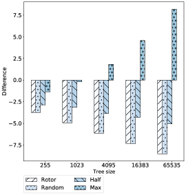
(a) $p=0.9$

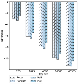
(b) $a=2.2$

Figure 2: Q1: Total cost difference of the self-adjusting algorithms minus Static-Oblivious, for high temporal ($p=0.9$) and spatial ($a=2.2$) locality.

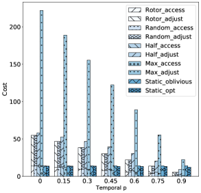
Figure 3: Q2: results for temporal locality. The x-axis shows the probability of repeating the last element and y-axis shows the costs.

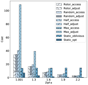
Figure 4: Q3: results for spatial locality. The x-axis shows the Zipf distributions parameters and the y-axis the average cost.

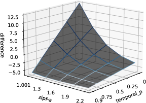
(a) Rotor-Push minus Static-Oblivious

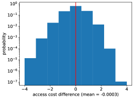
(b) Rotor-Push minus Random-Push

Figure 5: Q4: Rotor-Push performance. Figure 5a shows the difference of average cost between Rotor-Push and Static-Oblivious in combined scenarios of temporal and spatial locality of Q2 and Q3 (negative values have lighter color). Figure 5b shows a histogram of the access cost difference distribution per request between Rotor-Push and Random-Push, taken over ten sequences of uniform data. The mean is -0.0003 (marked with a red vertical line).

Q2: Temporal Locality. In Figure 4 we present our results for Q2. We plotted the total cost for each algorithm. We observe that Rotor-Push and Random-Push have the best performance and that all self-adjusting algorithms exploit temporal locality, as expected, but with varying efficiency. Interestingly, Rotor-Push and Random-Push outperform all other algorithms a bit after $p=0.75$, while Move-Half is only marginally more costly. On the other hand, the adjustment cost of Max-Push is quite high in all scenarios.

Q3: Spatial Locality. In Figure 4 we show our results for the spatial locality experiments. For the sequence of Zipf distributions with parameters $a\in(1.001,1.3,1.6,1.9,2.2)$, the respective average empirical entropies of the sequences that we sampled are $(11.07,6.47,3.88$, $2.63,1.92)$. That is, as $a$ increases, the sequences are more skewed, and the entropy decreases. Similarly to the temporal locality results, we observe that indeed all self-adjusting algorithms exploit spatial locality (Rotor-Push, Random-Push, and Max-Push have similar performance), and the reconfiguration cost pays off already from $a=1.6$ (when compared to Static-Oblivious). However, Static-Opt has the best performance in all scenarios.

Q4: Rotor-Push Performance. In Q4 we take a closer look on the performance of Rotor-Push, as in Q2 and Q3 it has the best performance, together with Random-Push. In Figure 5a we plot the total cost difference between Rotor-Push and the oblivious static initial tree (Static-Oblivious), in various scenarios of temporal and spatial locality. As expected, their combination has a more dramatic effect in cost reduction. Moreover, for ten sample sequences (each of length $10^{6}$) we observed (Figure 5b) that the difference between the cost of Rotor-Push and Random-Push is at most 4 (mean is $-0.0003$). Thus, the variance in their performance difference is also rather small (in the previous sections we observed that the means are almost equal).

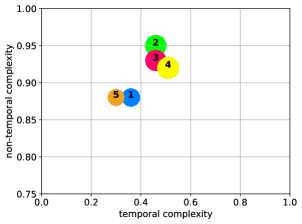
Figure 6: Q5: Complexity map [8] of the five datasets extracted from the five largest books in the corpus data.

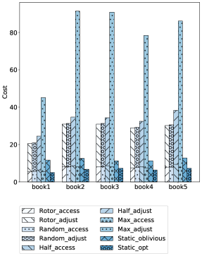
Figure 7: Q5: Performance of the corpus data.

Q5: Evaluation with corpus data. The complexity map computation [8] of the five datasets showed that their temporal complexity is in the interval $[0.3,0.5]$ and their non-temporal complexity is in the interval $[0.8,1]$ (Figure 7). This plot indicates that the datasets have moderate to high locality. In Figure 7 we plotted the performance of all six algorithms over these datasets. As in the synthetic data, we observe that (i) Rotor-Push and Random-Push are the best self-adjusting algorithms with similar performance, (ii) the access cost of Rotor-Push, Random-Push, and Move-Half is similar to the one of Static-Opt, and that (iii) the selected dataset doesn’t have high locality and hence the adjustment cost remains high.

6.3 Discussion

We discuss the main takeaways of our evaluation. From the plots that address Q1 we derived that in high locality scenarios, self-adjusting algorithms perform better as the network size increases, since the access cost for static algorithms increases as well (i.e. the tree size increases). We then fixed the tree size to 65,535 nodes (depth 15) and observed that the cost of adjustment pays off in high locality sequences (temporal, spatial, or combined). We observed that Rotor-Push and Random-Push have almost identical performance, both in synthetic and real data, despite their different properties. Recall that Random-Push has the working set property [11], but Rotor-Push doesn’t (cf. Section 4.3, Lemma 8). Specifically, even though the cost of Rotor-Push can be linear in the working set in theory, we did not observe this in any of the tested scenarios. Also, we found that the performance of all algorithms over corpus data follows the one observed with synthetic data.

7 Future Work

Our paper leaves open several interesting directions for future research. On the theoretical front, it would be interesting to provide tight constant bounds on the competitive ratio of our algorithm and the problem in general. On the applied front, it remains to engineer our algorithms further to improve performance in practical applications, potentially also supporting concurrency.

References

- [1] https://gitlab.com/robertsLab/pushdowneval.
- [2] H. Akbari and P. Berenbrink. Parallel rotor walks on finite graphs and applications in discrete load balancing. In Proc. 25th Annual ACM Symposium on Parallelism in Algorithms and Architectures (SPAA), pages 186–195, 2013.
- [3] S. Albers. Online algorithms: a survey. Math. Program., 97(1-2):3–26, 2003.
- [4] S. Albers and M. Janke. New bounds for randomized list update in the paid exchange model. In Proceedings of the International Symposium on Theoretical Aspects of Computer Science, STACS, volume 154, pages 1–17, 2020.
- [5] S. Albers and S. Lauer. On list update with locality of reference. In International Colloquium on Automata, Languages, and Programming, pages 96–107. Springer, 2008.
- [6] S. Albers and M. Mitzenmacher. Revisiting the counter algorithms for list update. Information processing letters, 64(3):155–160, 1997.
- [7] R. Arnold and T. Bell. A corpus for the evaluation of lossless compression algorithms. In Proceedings DCC’97. Data Compression Conference, pages 201–210. IEEE, 1997.
- [8] C. Avin, M. Ghobadi, C. Griner, and S. Schmid. On the complexity of traffic traces and implications. Proc. ACM Meas. Anal. Comput. Syst., 4(1), May 2020.
- [9] C. Avin, K. Mondal, and S. Schmid. Demand-aware network designs of bounded degree. In Proc. International Symposium on Distributed Computing (DISC), 2017.
- [10] C. Avin, K. Mondal, and S. Schmid. Push-down trees: Optimal self-adjusting complete trees. CoRR, abs/1807.04613, 2018.
- [11] C. Avin, K. Mondal, and S. Schmid. Dynamically optimal self-adjusting single-source tree networks. In LATIN 2020: Theoretical Informatics - 14th Latin American Symposium, pages 143–154, 2020.
- [12] C. Avin and S. Schmid. Renets: Statically-optimal demand-aware networks. In Proc. SIAM Symposium on Algorithmic Principles of Computer Systems (APOCS), 2021.
- [13] J. N. Cooper, B. Doerr, T. Friedrich, and J. Spencer. Deterministic random walks on regular trees. In Proceedings of the Nineteenth Annual ACM-SIAM Symposium on Discrete Algorithms (SODA), pages 766–772, 2008.
- [14] J. N. Cooper and J. Spencer. Simulating a random walk with constant error. Comb. Probab. Comput., 15(6):815–822, 2006.
- [15] I. Dumitriu, P. Tetali, and P. Winkler. On playing golf with two balls. SIAM Journal on Discrete Mathematics, 16(4):604–615, 2003.
- [16] M. L. Fredman. Generalizing a theorem of wilber on rotations in binary search trees to encompass unordered binary trees. Algorithmica, 62(3):863–878, 2012.
- [17] T. Friedrich and T. Sauerwald. The cover time of deterministic random walks. In International Computing and Combinatorics Conference, pages 130–139. Springer, 2010.
- [18] A. E. Holroyd and J. Propp. Rotor walks and markov chains. Algorithmic probability and combinatorics, 520:105–126, 2010.
- [19] J. Iacono. Key-independent optimality. Algorithmica, 42(1):3–10, 2005.
- [20] S. Kamali and A. López-Ortiz. A survey of algorithms and models for list update. In Space-Efficient Data Structures, Streams, and Algorithms - Papers in Honor of J. Ian Munro on the Occasion of His 66th Birthday, volume 8066 of Lecture Notes in Computer Science, pages 251–266. Springer, 2013.
- [21] I. Landau and L. Levine. The rotor–router model on regular trees. Journal of Combinatorial Theory, Series A, 116(2):421–433, 2009.
- [22] A. López-Ortiz, M. P. Renault, and A. Rosén. Paid exchanges are worth the price. Theor. Comput. Sci., 824-825:1–10, 2020.
- [23] J. I. Munro. On the competitiveness of linear search. In Proceedings of the European Symposium, ESA, volume 1879, pages 338–345, 2000.
- [24] V. B. Priezzhev, D. Dhar, A. Dhar, and S. Krishnamurthy. Eulerian walkers as a model of self-organized criticality. Physical Review Letters, 77(25):5079, 1996.
- [25] N. Reingold, J. R. Westbrook, and D. D. Sleator. Randomized competitive algorithms for the list update problem. Algorithmica, 11(1):15–32, 1994.
- [26] S. Schmid, C. Avin, C. Scheideler, M. Borokhovich, B. Haeupler, and Z. Lotker. Splaynet: Towards locally self-adjusting networks. IEEE/ACM Transactions on Networking, 24(3):1421–1433, 2015.
- [27] K. Siegrist. Probability, mathematical statistics, stochastic processes, 2017.
- [28] D. D. Sleator and R. E. Tarjan. Amortized efficiency of list update and paging rules. Communications of the ACM, 28(2):202–208, 1985.
- [29] D. D. Sleator and R. E. Tarjan. Self-adjusting binary search trees. Journal of the ACM (JACM), 32(3):652–686, 1985.
- [30] I. A. Wagner, M. Lindenbaum, and A. M. Bruckstein. Distributed covering by ant-robots using evaporating traces. IEEE Transactions on Robotics and Automation, 15(5):918–933, 1999.