Risk Awareness in HTN Planning

Abstract

Actual real-world domains are characterised by uncertain situations in which acting and use of resources require embracing risk. Performing actions in such domains always entails costs of consuming some resource, such as time, money, or energy, where the knowledge about these costs can range from totally known to totally unknown and even unknowable probabilities of costs. Think of robotic and marine domains, where actions and their costs are non-deterministic due to the uncertainty of factors, such as obstacles and weather conditions. Choosing which action to perform considering its cost on the available resource requires taking a stance on risk. Thus, these domains call for not only planning under uncertainty but also planning while embracing risk. Taking Hierarchical Task Network (HTN) planning as a widely used planning technique in real-world applications, one can observe that existing approaches do not account for risk. That is, computing most probable or optimal plans using actions with single-valued costs is only enough to express risk neutrality. In this work, we postulate that HTN planning can become risk aware by considering expected utility theory, a representative concept of decision theory that enables choosing actions considering a probability distribution of their costs and a given risk attitude expressed using a utility function. In particular, we introduce a general framework for HTN planning that allows modelling risk and uncertainty using a probability distribution of action costs upon which we define risk-aware HTN planning as an approach that accounts for the different risk attitudes and allows computing plans that go beyond risk neutrality. In fact, we lay out that computing risk-aware plans requires finding plans with the highest expected utility. Finally, we argue that it is possible for HTN planning agents to solve specialised risk-aware HTN planning problems by adapting some existing HTN planning approaches.

1 Introduction

The innovator’s dilemma is the hard decision organisations face when they have to choose between sustaining innovation or accepting disruptive innovation [1]. Are they ready to give up the innovations they have made and invest in the unknown? Accepting disruptive innovation requires changing established attitudes that focus on security and aversion towards taking chance when it comes to decision making and resource allocation. We can, thus, say that the innovator’s dilemma is all about embracing risk in the presence of uncertainty.

The innovator’s dilemma is also applicable to domains other than the business one. In general, real-world domains are typically non-deterministic and exhibit a wide-ranging spectrum of uncertainty, requiring planning and decision making processes to embrace risk in one form or another. In this context, decision theory offers mechanisms to rank options on how choice-worthy they are. The most representative mechanism is expected utility theory, which sets a fundamental principle by which decisions are made in environments, that have a probability distribution over action costs, according to a given risk attitude [2].

The requirement for planning and decision making processes to embrace risk in the presence of uncertainty also holds when automating the processes of decision making, which is of primary concern of Artificial Intelligence Planning.

In its simplest form, AI planning is about the generation of a course of action whose execution in an initial state of the world satisfies some user objective. In AI planning, uncertainty is considered in the initial state and actions in the form of incomplete knowledge and multiple effects of actions, possibly with probability of their execution.

The concept of risk, however, has not been treated much despite the fact that there are planning problems in which performing actions always incurs costs on a resource of interest, such as money, time, energy, and/or effort. For some problems, it might be preferred to accept plans with larger execution costs in order to avoid risk. For others, risky plans are preferred if they promise, even with a low probability, lower execution costs. The current practice that actions have unit cost of typically one unit does not reflect reality. Action costs are not static, cannot be easily predefined, and sometimes cannot be even predicted reliably. Take, for example, the domain of smart buildings, which are buildings connected to the smart grid and equipped with intelligent automation systems with the objective of maintaining economical and environmental sustainability. When it comes to electricity, smart buildings can nowadays get energy from two different sources, that is, local renewable resources and electric utilities with varying prices and energy offers [3]. To achieve their objective, these buildings need to plan the energy demand and supply, which requires, among other things, choosing energy actions under risk related to the costs of these actions due to uncertainties in the market prices and weather forecasts. In general, the uncertainty spectrum starts at totally known probability distribution over action costs and ends at totally unknown and even unknowable costs and probabilities [4]. Similarly to having actions with multiple effects, having this variability of action costs can lead to plans of a probabilistic nature. That is, the resource consumption of the same plan can differ from one plan execution to another. Thus, it is of utmost importance to compute plans that embrace risk by taking the variability of action costs into account. As a result, the quality of plans plays a role when planning under risk.

1.1 HTN Planning and Its Risk Neutrality

Among AI planning techniques, Hierarchical Task Network (HTN) planning is a widely used one in real-world domains, such as Web service composition, e.g, [5], games, e.g. [6], robotics, e.g. [7], healthcare, e.g., [8], cloud computing [9], building automation [10]. This technique is essentially based on the idea of enriching planning domains with knowledge on how to accomplish tasks in some domain [11, 12]. This rich domain knowledge and its intrinsic hierarchical structure enable HTN planning to provide a natural approach to simulate the way in which one conceptualises performs decision making in domains that involve risk. In particular, HTN planning requires an initial state, an initial task network as an objective to be accomplished, and domain knowledge consisting of networks of primitive and compound tasks. A task network represents a hierarchy of tasks each of which can be directly executed, if the task is primitive, or decomposed via methods into subtasks, if the task is compound. One way to search for solutions is to start decomposing the initial task network and continue doing it until all compound tasks have been decomposed. The solution is a plan which equates to a set of primitive tasks applicable to the initial state, if it exists.

In the realm of uncertainty, there are HTN planning approaches that deal with probabilistic plans and differ in what selection criteria each approach uses to rank plans. Some planning approaches do not consider action costs, but rather consider probabilistic effects of actions. These approaches aim at finding plans with the highest probability of success, e.g., [13]. Other approaches do take action costs into account, but aim at finding plans that have the highest probability of not exceeding a predefined cost limit, e.g., [14]. There are even approaches that assume the world is deterministic and assign a single real-valued number to each action to quantify its resource consumption [15, 16]. Such approaches usually aim at computing cost-optimal plans, where the plan’s cost is the total sum of the costs of its constituent actions.

In general, an agent acting on the basis of such HTN planning approaches is indifferent to the risk that may arise due to the made planning choices. Thus, this planning agent is risk neutral. And the working and objectives of risk-neutral HTN planning agents do not entirely meet the expectations for decision makers in actual settings. Decision making and planning in real-world situations requires embracing the risk.

1.2 Proposal and Contributions

We posit that risk awareness of HTN planning can be achieved by considering expected utility theory. Specifically, we draw on the view of expected utility theory towards rationality when making decisions under risk to suggest that different risk attitudes can be incorporated in HTN planning.

The risk attitudes are expressed using utility functions that map operator costs into real values provided there is a variability of those costs. This enables us to propose a definition of risk-aware HTN planning in which plans have the maximum expected utility and computed by making informed planning choices. As a result, the quality of plans or risk awareness of plans emerges.

The contributions of the present article are:

• We provide a broader perspective of uncertainty and risk, where we define uncertainty and risk as two distinct concepts. We mainly draw knowledge from decision theory and its established mechanisms for embracing risk when making decisions. This opens the pathway for the presentation of our main technical contributions to AI Planning.

• We identify the sources of uncertainty in relation to costs of actions and position them with respect to the available knowledge from decision theory.

• We provide a general framework of HTN planning for uncertainty and risk based on the variability of action costs. While the framework builds upon an existing HTN planning formalism, to the best of our knowledge, it represents the first general approach that accounts for variability of action costs. While this enables us to define our risk-aware HTN planning, it also represents a stepping stone for new approaches.

• We propose the novel concept of risk-aware HTN planning, which is capable of embracing risk in real-world domains for which HTN planning is a fit. This concept is inspired by our preliminary idea [17], and, to the best of our knowledge, represents the first work that incorporates risk in HTN planning and it does so upon established concepts from decision theory. Risk-aware HTN planning paves the way to having more specific risk-aware HTN planning problems and constructing algorithms that can solve them.

• We go one step further and suggest possible ways to solving risk-aware HTN planning problems under some simplifying assumptions by adapting existing HTN planning approaches. We do this for both models of HTN planning, namely state-based HTN planning and plan-based HTN planning.

• We provide a wider overview of works that deal not only with planning under uncertainty and risk but also with mechanisms that do not relate to risk but do support informed decision making in HTN planning.

1.3 Organisation

The remainder of the article is organised as follows. Section 2 presents the perspective of uncertainty and risk as seen from decision theory. Section 3 introduces sources of uncertainty and its effects on action costs. Section 4 presents the formalism of the general framework we propose, while Section 5 introduces risk-aware HTN planning. Section 6 gives insights into some possible approaches for solving specific risk-aware HTN planning problems. Section 7 provides an overview of the related work, while Section 8 includes a discussion on selected questions related to our proposal. Section 9 finalises the article with concluding remarks.

2 Uncertainty and Risk in a Broader Perspective

Individuals are continuously confronted with situations that necessitate making decisions. If for simple situations, an immediate and intuitive course of action suffices; in more intricate situations more options will be available and the effects of initial choices on subsequent states will be uncertain and largely hard to intuitively predict.

2.1 General definitions

To systematise decision making, research in various fields have been carried out with the aim of providing decision makers with conceptual understanding and methodical ways to analyse and reason about different alternatives. In decision theory, two factors have been identified that increase the complexity of decision-making problems, namely uncertainty and risk [18].

The awareness about the distinction between uncertainty and risk has been present for decades in the field of economics. In 1921, Frank H. Knight made an explicit distinction between uncertainty and risk in his classic of economic theory presented in [19]. Knight defines uncertainty as a decision-making situation in which the likelihoods of alternative outcomes are unknown to the decision maker or are impossible to form, i.e., incalculable due to their uniqueness or due to their irregularity. Risk, on the other hand, is present when all outcomes and their probability of occurrence are known either a priori or from statistics gathered from past experience.

Similar knowledge can be found in game theory, where decision making is classified according to whether it is affected by certainty, uncertainty, and risk [22]. Certainty is defined as the situation in which the decision maker knows the exact outcome of alternatives, while uncertainty and risk are defined similarly to Knight’s definitions.

Knight’s distinction between uncertainty and risk has been further refined into a taxonomy that captures the relation between uncertainty and risk in physics [4]. The uncertainty taxonomy provides a wide spectrum of uncertainty formulated in five levels as illustrated in Figure 1. These levels range from complete certainty to irreducible uncertainty:

• Level 1 defines complete certainty, i.e., nothing is uncertain.

• Level 2 defines risk without uncertainty, where outcomes and their probability distribution are known.

• Level 3 defines fully reducible uncertainty, where the outcomes are fully known, but their probability distribution is unknown. The uncertainty in this level is fully reducible to risk by statistical inference of the probability distribution of outcomes.

• Level 4 is partially reducible uncertainty, where there is a limit to what we can deduce about the outcomes and their probability even by significant statistical inference, and a significant amount of the outcomes and their probabilities are uncertain, which leads to model uncertainty. The probabilities in this level reflect beliefs rather than frequencies of repeated trials as defined in Levels 2 and 3.

• Level 5 defines irreducible uncertainty, which is the state of total ignorance that cannot be solved by collecting more data nor using sophisticated methods of statistical inference.

Figure 1: Uncertainty taxonomy from [4] mapped to Knight’s definitions of risk and uncertainty and vNM’s and Savage’s theorems.

Figure 1 shows our mapping of Knight’s definition of risk to Levels 2 and 3, and his definition of uncertainty to Level 4. In this context, our work adopts the distinction of uncertainty and risk, and furthermore, defines risk as a combination of Knight’s definition with Levels 2 and 3 of the uncertainty taxonomy, and uncertainty as a combination of Knight’s definition with Level 4 of the taxonomy.

Definition 2.1 (Risk).

Risk is a decision-making situation in which either all outcomes and their probability of occurrence are known a priori or the probability distribution of outcomes is unknown but can be deduced using statistical inference.

Definition 2.2 (Uncertainty).

Uncertainty is a decision-making situation in which either there is a limit to what can be deduced about the probability distribution of alternative outcomes, where the probabilities represent degrees of decision maker’s beliefs, or the probability distribution is not only unknown but also unknowable.

2.2 Uncertainty and Risk Through the Concept of Utility

Risk and uncertainty play a central role in making rational decisions. Let us look at this through the lenses of utility theory: the most representative theory in decision making that explains the acts of rational choices using the concept of utility. More specifically, utility theory provides a mathematical framework for modelling decision making under risk and uncertainty and explains people’s behaviour on the premise that people can rank choices based on their preferences in terms of the satisfaction of all decision outcomes [23].

We show that the distinction between risk and uncertainty is useful to divide theories of choice in expected utility theory, an axiomatic theory of choice, into theories that deal with decisions under risk and others that deal with decisions under uncertainty [24]. We explain the existence of rationality in decision making and how this can be expressed in different attitudes toward risk using utility functions.

2.2.1 Rationality in Decision Making

In 1738, Daniel Bernoulli posited the expected utility theory by making a clear distinction between the expected value and the expected utility, as the latter uses weighted utility, the value of the outcome to the decision maker, multiplied by probabilities instead of using weighted outcomes. The theory was first axiomatised and mathematically formulated by von Neumann and Morgenstern (vNM) in 1944 [2]. They formulated what is known as the vNM Theorem which suggests that maximising the expected utility is the objective of a rational agent, where the decision maker’s preference structure over outcomes is assumed, utilities of outcomes are known, and the decision maker knows the “objective” probability of outcomes. A utility measures the subjective worth of an outcome, whether it is a monetary value or any other type of value, by mapping outcomes to real-valued utilities using a utility function. The utility function formalises the decision maker’s preference structure. The expected utility is the sum of the utilities of outcomes weighted by the corresponding probabilities. Since the theorem assumes “objective” utilities are known, it incorporates the notion of risk through the expected utility theory.

Savage’s theorem is considered the generalisation of the vNM theorem and it approaches decision making under uncertainty [25]. The theorem suggests that a rational decision maker makes choices as if she/he is maximising the expected utility using a “subjective” probability distribution, which is a translation of the decision maker beliefs about the outcomes and is different from one decision maker to another.

Considering the taxonomy of risk and uncertainty from Section 2.1, we can map the different taxonomy levels to the two theorems of expected utility as illustrated in Figure 1. The vNM theorem focuses on decision making situations that involve either risk or uncertainty that is fully reducible to risk, i.e., Levels 2 and 3 of the taxonomy. Savage’s theorem, on the other hand, addresses situations that involve partially reducible uncertainty, where the probability of the outcomes represent the decision maker’s beliefs, i.e., Level 4 of the taxonomy.

2.2.2 Risk Attitudes

In the world of uncertainty and risk, agents make decisions that reflect a specific risk attitude, which defines people’s mindset towards taking risk. Some decision makers have a simple objective of minimising expected loss. These decision makers are indifferent to the risk involved in the various choices and they focus solely on the expected loss each alternative entails. In other words, they are risk neutral. However, in domains that are characterised by huge wins or losses, that is, high-stake domains, decision makers have objectives that go beyond minimising expected costs to account for the degree of risk associated with each choice. In reality, decision makers are seldom risk neutral. In fact, decision makers might be risk averse, i.e., they avoid risky choices that can expose them to a high degree of loss. For example, risk-averse decision makers will always choose to insure valuable assets, such as homes and cars, to avoid the potential loss of these assets. Although the probability of a loss may be small, the potential loss of the asset itself would be very large. Thus, these individuals are willing to rather pay a monthly fee to insurance companies rather than face the risk of potential losses.

The opposite of the risk-averse attitude is the risk seeking one. Decision makers with this attitude tolerate losses more than the risk-averse individuals and prefer risky alternatives that have the potential of high returns. Thus, when they are offered two choices with the same expected utility, they prefer the risky choice if it has the potential of higher returns. For example, if a risk seeking individual is given the choice between a gamble and a sure outcome, s/he prefers the gamble if there is a possibility of higher returns.

2.2.3 Dynamics of Risk Attitudes

Risk attitudes of decision makers usually follow one of two patterns, static or dynamic. Decision makers have a static risk attitude when their attitudes do not change by time and are not affected by any factor, such as their wealth level. On the other hand, some decision makers have a dynamic risk attitude that changes with some factors, such as the wealth level or the decision-making history of the decision maker. For example, there are studies that statistically prove that the income of a decision maker is positively related to her/his risk attitude. This means that an increase in the decision maker’s income increases the odds of him/her being risk-seeking and a decrease in an income increases the odds of the decision maker being risk-averse [26]. Arguments exist that most people are risk-averse when they have a small amount of money, and become more and more risk-neutral when they get richer and richer [27, 28]. This property of switching attitude was proposed in [29] and studied further in [30]. [28] give an example of such behavior where a contestant in the TV show “Who Wants to be a Millionaire” has reached the one million dollar question, for which s/he does know the answer, and s/he has two alternatives to choose from. S/He can either leave with $500,000 for sure, or guess the answer and then win $1,000,000 with 50% probability (if the answer is correct) and $32,000 with 50% probability (if the answer is wrong). For average people, the rewards are high compared to their wealth. Thus, they are expected to be risk-averse and leave. However, if the contestant is a billionaire, the wealth levels are low compared to her/his wealth. Thus, it is expected that s/he chooses to answer the question.

The history of the decision maker is another factor that can influence the dynamics of his/her risk attitude. A history-dependent risk-aware model for decision making defines a behavioural model in which the decision maker’s risk attitude changes based on his/her history of disappointments and elation [31]. To determine whether an outcome of a certain choice is disappointing or elating, the decision maker assigns a threshold above which the outcome is considered elating or disappointing otherwise. This history of elation and disappointments reinforces the risk attitude of the decision maker, i.e., the decision maker’s risk aversion decreases after elating experience and increases after disappointing one. In addition, the decision makers are proved to show a primacy effect. The primacy effect indicates that the sequence of outcomes matters, i.e., the earlier the decision maker is disappointed, the more risk averse she/he becomes. This behavioural model is evident in a variety of real-world domains. For example, after the 2008 financial crisis in Italy, Italian investors showed a substantial increase in their risk aversion during risky gambles compared to their risk attitudes before the the crisis [32]. Examples from other studies show how the primacy effect plays a big role in shaping the risk attitude of decision makers can be found in [33, 34].

2.2.4 Utility Functions

Risk attitudes of decision makers are determined by utility functions. In particular, each decision maker has a strictly monotonically non-decreasing utility function that transforms the real-valued outcomes into real-valued utilities. The decision maker always tries to maximise his/her expected utility under a set of axioms.

For decision makers who are not risk sensitive, i.e., they are risk neutral, the utility function is linear, and, thus, their behavior is reward maximisation (in gain domains) or cost minimisation (in loss, i.e., cost-based domains). On the other hand, if the decision maker is risk sensitive, their utility function is non-linear, for instance it could be exponential. If the utility function is concave, the decision maker is risk averse, while if the utility function is convex, the decision maker is risk seeking. Such utility functions express the static risk attitude of decision makers.

To model dynamic risk attitudes, a different type of utility functions should be used. For example, Bell [29] and Bell and Fishburn [30] discuss a class of utility functions that can be used to express the switch in the decision maker’s attitude with the change of his/her wealth level. The utility functions belonging to this class are called $m$-switch utility functions, where $m$ is the number of switches in the attitude. Then, the zero-switch utility functions are the utility functions that express static risk attitudes. The mostly used utility function from this class is the one-switch utility function, which expresses that for every pair of alternatives whose ranking is not independent of the wealth level, there exists a wealth level above which one alternative is preferred, below which the other is preferred. This utility function is a linear combination of linear and exponential utility functions [27, 35]. In addition to the studies that focus on wealth-dependent risk attitudes, there are studies that focus on studying utility functions that are dependent on other factors. For example, one can find utility functions for history-dependent risk awareness in [31].

3 Sources and Effects of Uncertainty

To fulfil our objective of creating a general framework for HTN planning under uncertain situations, we start by studying the sources of uncertainty in real-world domains and their effects on the execution costs of actions.

3.1 Sources of Uncertainty

One important factor that planning agents, i.e., the decision makers in an autonomous system, need to account for when planning in real-world domains is the source of uncertainty. In turn, to understand the sources of uncertainty, it is important to know what type of agents operate in a given domain, what we refer to as executing agents. More specifically, we distinguish two types of executing agents. The first type is human beings, where a human is either instructed by the planning agent to execute actions or act based on his/her free will, while the second type is a system, which represents any type of executors that are not human beings, e.g., robots and actuators.

Given these types of executing agents, we can refine and categorise the sources of uncertainty that planning agents should consider in three categories. The first and second categories include sources of uncertainty when the executing agent is a system and when it is a human, respectively. The third category considers source of uncertainty in domains where both systems and humans can execute actions. Figure 2 depicts these categories of sources of uncertainty.

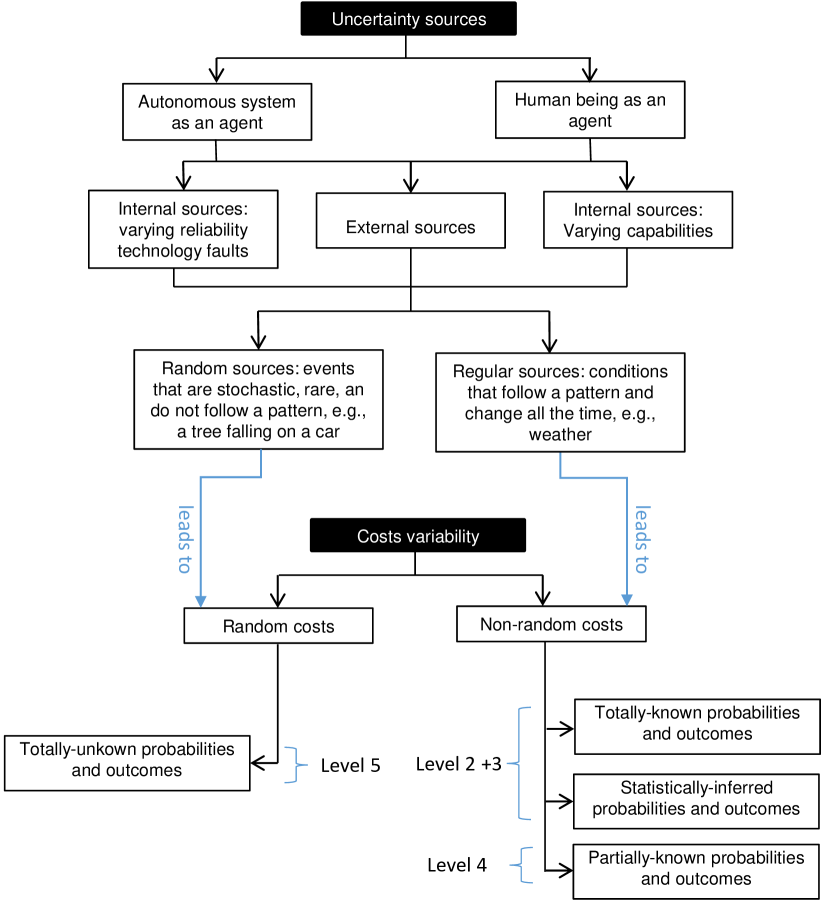
Figure 2: Categorisation of uncertainty sources and their effects on action costs.

In each category, we further distinguish two types of sources of uncertainty, namely internal sources and external sources. Internal sources are those caused by the agent itself either due to uncertain behaviour of the agent, variable capabilities of the agent, or due to malfunctioning of the whole agent or parts of it. The external sources, on the other hand, are sources of uncertainty caused by the environment surrounding the agent and independent of the agent’s actions. Each type of source is further categorised into random sources and regular sources. Random sources of uncertainty are events that are stochastic, rare, and do not follow a pattern. Regular sources are conditions that follow some pattern and change all the time within the agent itself, in case of internal sources, or within the surrounding environment, in case of external sources. For illustrations of these sources, see A.

The sources on uncertainty reported here are related to the uncertainty dimensions presented in [36]. In particular, there are three dimensions of uncertainty: (1) unexpected events, which are the events that happen in exceptional and unpredictable situations, (2) actions contingencies, which can be either failures or timeouts, and (3) partial observability, which refers to the imperfectness and incompleteness of information about environment states. The first dimension is related to the random sources of uncertainty. The second and third dimensions, however, are relevant to all uncertainty sources in our categorisation. In particular, the sources of uncertainty, internal or external, can result in incomplete or imperfect information. Similarly, the failure of actions can be relevant to internal sources caused by the unreliability of the agent, or external sources, random or regular.

3.2 Effects of Uncertainty on Action Costs

Performing actions changes the state of the environment and incurs costs in terms of money, time, fuel, or effort. In the world of certainty, these costs are deterministic. However, with the inclusion of uncertainty, actions have uncertain costs. In particular, the exact costs of performing actions are not necessarily known with certainty at the time of planning, because most often actions are not guaranteed to have the same execution cost every time they are executed. In other words, actions have variable costs. To capture this fact, we call actions in uncertain domains cost-variable actions.

The effects of uncertainty, i.e., the variability of action costs, can be also categorised based on the sources of uncertainty as illustrated in Figure LABEL:fig:cost-variability. When the uncertainty exists because of random sources, the variability of costs is unpredictable, which means it cannot be modelled in advance or dealt with during offline planning. This kind of cost variability corresponds to Level 5 of the uncertainty taxonomy shown in Figure 1. On the other hand, when uncertainty is caused by regular sources, the variability of costs can be further described by two categories. The first category corresponds to Level 2 and Level 3 of the uncertainty taxonomy, where the costs and their probability distribution are either known or can be statistically inferred. We call actions in this category risk-inducing actions. We call the domains that contain this kind of actions risk-involving domains. The second category corresponds to Level 4 of the uncertainty taxonomy and includes actions that have a probability distribution representing the decision maker’s beliefs. We call actions from this category uncertainty-inducing actions. Similarly, we call the domains that contain this kind of actions uncertainty-involving domains. This categorisation of cost variability is applied to actions that have a single effect on the environment or multiple uncertain effects. In other words, an action can have either a deterministic effect that always changes the state in one way but with variable costs, or multiple uncertain effects with variable costs.

4 A Framework of HTN Planning with Uncertainty and Risk

To set the foundations for HTN planning with uncertainty and risk, we need a formal framework of HTN planning upon which we can build and incorporate the concepts of uncertainty and risk. To this end, we begin with presenting such formal framework of classical HTN planning for state-based HTN planning [11]. As providing also a formalism on plan-based HTN planning (that is, decomposition-based HTN planning) would unnecessarily complicate our presentation, we refer the reader to the formalism of plan-based HTN planning in [11] or decomposition-based HTN planning in [12].

These two models differ in the search space the HTN planning process operates in [11, 37, 12]. In plan-based HTN planning, the search space consists of task networks. The search starts at an initial task network and each decomposition of a compound task creates a new task network. Decomposing compound tasks is repeated until all compound tasks are decomposed, i.e., a primitive task network is reached. Each task network in the planning space is considered a partial plan. The solution is then a linearisation of the primitive task network.

Having partial plans as search nodes potentially leads to a more compact—but also more complex—representation of the search space when compared to state-based planning. However, since the state is not progressed in this model, the planner does not have information about the current state of the world during planning.

On the other hand, in state-based HTN planning, the search space consists of subset of the state space that is restricted by task decompositions. The search starts at an initial state with an empty plan. The goal is to compute a plan by searching for a state that accomplishes the initial task network. During search, when encountering a compound task, if there is an applicable method, that task is decomposed. Then, the task decomposition continues on the next decomposition level but in the same state. If the task is primitive, it is executed, removed from the task network, and added to the plan. The search then continues into a successor state.

4.1 Classical HTN Planning

A HTN planning problem is a 3-tuple $P=\langle s_{0},tn_{0},D\rangle$, where $s_{0}$ is the initial state, $tn_{0}$ is a task network, called initial task network, and $D$ is a planning domain consisting of a set of operators and methods. A task network is a pair $\langle T_{n},\prec\rangle$, where $T_{n}$ is a set of tasks and $\prec$ is a partial order over $T_{n}$. Tasks in $T_{n}$ can be either primitive or compound. A task is primitive if it can be accomplished directly by an operator $o=\ \langle pt(o),pre(o),\mathit{eff(o)}\rangle$, where $pt(o),pre(o),$ and $\mathit{eff(o)}$ are the operator’s name, precondition, and effects, respectively. The operator’s name is identical to the primitive task that can be executed by this operator. There is a one-to-one mapping between operators and primitive tasks. A task is said to be compound if it must be decomposed into smaller sub-tasks using a method $m=\langle ct(m),pre(m),tn(m)\rangle$, where $ct(m),pre(m)$ and $tn(m)$ are the method’s name, precondition and the method’s task network, respectively. The method’s name represents the compound task it can decompose. One compound task can be decomposed by multiple methods. In state-based HTN planning, the planning process starts by decomposing the initial task network and continues until all compound tasks are decomposed. Decomposing a compound task requires that at least one of the methods that can decompose it be applicable, i.e., the precondition of the method is fulfilled in the current state of the world. Similarly, executing a primitive task requires that the corresponding operator be applicable. The solution to $P$ is a plan $\pi=\langle o_{1},o_{2},\ldots,o_{n}\rangle$ which equates to a set of operators applicable to the initial state and can accomplish the initial task network.

Since HTN planning constructs form a hierarchical structure, intuitively, they can be represented using graphs. This representation makes it easier for us to extend the classical HTN planning framework and to incorporate risks and uncertainties by mapping it to established techniques in decision making, such as decision trees, as we explain later. So, to represent domain descriptions, we adapt the definition of the Task Decomposition Graph (TDG) from [38]. TDG is a graph in which vertices represent both tasks and methods, and the directed edges go from a task vertex to all method vertices that can decompose it and from a method vertex to all task vertices in its task network.

Definition 4.1 (Task Decomposition Graph).

Let $D=\ \langle O,\ M\rangle$ be an HTN planning domain. The bipartite directed graph $G=\ \langle V_{T},V_{M},E_{T\to M},E_{M\to T}\rangle$, where $V_{T}$ is a set of task vertices, $V_{M}$ is a set of method vertices, and $E_{T\to M},\ E_{M\to T}$ are sets of edges, is a Task Decomposition Graph (TDG) of D if and only if:

1. $\forall m=\langle ct(m),pre(m),tn(m)\rangle\in M$:

   • $v_{t}\in V_{T}$ such that $v_{t}=ct(m)$, and

   • $v_{m}\in V_{M}$ such that $v_{m}=m$, and

   • $(v_{t},v_{m})\in E_{T\to M}$, and

   • $\forall t_{i}\in tn(m)$: $v_{t_{i}}\in V_{T}$ and $(v_{m},v_{t_{i}})\in E_{M\to T}$ such that $v_{t_{i}}=t_{i}$ .

2. $G$ is minimal, such that (1) holds true.

4.2 HTN Planning with Cost-Variable Operators

In Section 3, we argue that the variability of action costs in real-world domains constitutes a source of uncertainty and risk, which are intrinsic properties of these domains. Therefore, planning requires the concepts of risk and uncertainty to be explicitly modelled and taken into account generating the plans.

Variability of costs can be modelled as a probability distribution over the possible costs of operators. To be more specific, recall first that variability of costs can appear in two types of actions, risk-inducing and uncertainty-inducing actions (see Section 3). Then, to model risk-inducing actions, one needs to encode the probability distribution obtained from past experience or from statistical inference over the operator costs. These operators correspond to Level 2 and Level 3 of the uncertainty taxonomy (see Figure 1). We call such operators risk-inducing operators. Whereas to model uncertainty-inducing actions, the probability distribution over operator’s costs is modelled as a representation of the beliefs of the agent. Similarly, these operators are mapped to Level 4 of the uncertainty taxonomy. We call such operators uncertainty-inducing operators.

We now extend the classical HTN planning framework to account for variable-cost actions. To achieve this, we define operators with probabilistic effects and costs.

Definition 4.2 (Cost-Variable Operator).

A cost-variable operator $o$ is defined as a tuple $o=\ \langle pt(o),pre(o),\mathit{eff(o)},c(o)\rangle$, where $pt(o)$, and $pre(o)$ are defined as before, and $\mathit{eff(o)}$, and $c(o)$ are tuples that represent the effects and the costs of the operator, respectively and are defined as follows. $\mathit{eff(o)}=\langle(p_{1}(o),\mathit{eff_{1}(o)}),(p_{2}(o),\mathit{eff_{2}(o)}),\cdots,(p_{n}(o),\mathit{eff_{n}(o)})\rangle$ and $c(o)=\langle(p_{1}(o),c_{1}(o)),(p_{2}(o),c_{2}(o)),\cdots,(p_{n}(o),c_{n}(o))\rangle$, such that $\mathit{eff(o)}$ are the variable effects of the operator and $c(o)$ is the variable costs of the operator $c(o)=\langle(p_{1}(o),c_{1}(o)),(p_{2}(o),c_{2}(o)),\cdots,(p_{n}(o),c_{n}(o))\rangle$

• $\mathit{eff_{i}(o)}$ and $c_{i}(o)$ are the $i$th effect with its corresponding cost, respectively

• $\forall n>0\ \forall i\in[1,n],\ 0<p_{i}(o)<1$

• $\sum\limits_{i=1}^{n}p_{i}(o)=1$

• $c_{i}(o)<0$

Since we are dealing with a cost-based domain, we assume in our definition that costs have negative values. However, the definition can be easily generalised to model costs as positive values, to have rewards instead of costs, or to model any function of both rewards and costs.

We can now reflect our extended formalism on the definition of the TDG. We refer to the resulting TDG as Cost-Variable Task Decomposition Graph (CV-TDG).

Definition 4.3 (Cost-Variable Task Decomposition Graph).

Let $D=\ \langle O,\ M\rangle$ be an HTN planning domain, where $O$ is a set of cost-variable operators. The directed graph $G=\ \langle V_{TC},V_{TP},V_{M},E_{TC\to M},E_{M\to TC},E_{M\to TP}\rangle$, where $V_{TC}$ is a set of compound task vertices, $V_{TP}$ is a set of primitive task vertices, $V_{M}$ is a set of method vertices, and $E_{TC\to M},E_{M\to TP}$, and $E_{M\to TP}$ are sets of edges, is a Cost-Variable Task Decomposition Graph (CV-TDG) of D if and only if:

1. $\forall m=\langle ct(m),pre(m),tn(m)\rangle\in M$:

   • $v_{tc}\in V_{TC}$ such that $v_{tc}=ct(m)$

   • $v_{m}\in V_{M}$ such that $v_{m}=m$

   • $(v_{tc},v_{m})\in E_{TC\to M}$

   • $\forall t_{p}\in tn(m)$: $(v_{m},v_{tp})\in E_{M\to TP}$ such that $v_{tp}=t_{p}$

   • $\forall t_{c}\in tn(m)$: $(v_{m},v_{tc})\in E_{M\to TC}$ such that $v_{tc}=t_{c}$

2. $\forall o=\langle pt(o),pre(o),eff(o),c(o)\rangle\in O$

   • $v_{tp}\in V_{TP}$ such that $v_{tp}=o$

   • $\exists$ cost function c: $c:v_{tp}\rightarrow c(o)$

3. $G$ is minimal, such that (1) and (2) hold true.

Figure 3 shows an example of CV-TGD for an abstract HTN domain with four compound tasks and ten primitive tasks. The graph has three types of vertices labelled with $v_{tc_{i}}$, $v_{tp_{j}}$, and $v_{m_{k}}$ to represent compound tasks, primitive tasks, and methods vertices, respectively. Costs and effects variability are illustrated under the corresponding primitive tasks by probabilities $p_{l}$, effects $\mathit{eff_{l}}$, and costs $c_{r}$.

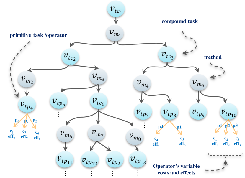
Figure 3: Cost-Variable Task Decomposition Graph (CV-TDG) representation of an abstract domain description. Compound tasks, primitive tasks, and methods are referred to as $v_{tc_{i}}$, $v_{tp_{j}}$, and $v_{m_{k}}$, respectively. The cost and effect variability of operators is illustrated under the corresponding primitive tasks by probabilities $p_{l}$, effects $\mathit{eff_{l}}$, and costs $c_{r}$.

5 Risk-Aware HTN Planning

While decision theory provides a theoretical framework on how to make decisions when confronted with multiple choices in the existence of risks, it does not tell us how to construct solutions. This is where AI panning, and HTN planning in particular, comes into play. We show what kind of planning decisions are needed in HTN planning and how concepts from decision theory can be used to make these decisions. We also lay the foundations for HTN planning that can solve planning problems in real-world domains characterised by risk. We reflect the concept of risk-aware decision makers and risk attitudes on HTN planning agents. Thus, our proposal and discussion are directed to planning in real-world domains that have risk-inducing actions, which are a result of internal and external regular sources of uncertainty. This means that the vNM theorem is applicable for these planning problems. To simplify our discussion, we focus on risk-inducing actions with a single effect.

5.1 Risk in Planning Decisions

There are three types of planning decisions that should be made during the HTN planning process. The first type represents the choice of a method to use when decomposing a compound task. The second is about the choice of values that are assigned from the problem definition to the domain parameters, or bindings. The third is about deciding the order in which compound tasks in the method task network are chosen. The last type of choices is only applicable in partially ordered and unordered state-based HTN planning [11]. These planning choices eventually influence the outcome of the planning process.

To exemplify these planning decisions, we illustrate a model of the domain of marine environments described in more details in A.3. In the scenario, there are two ways to collect ocean data: a diver can dive alone or a glider can accompany the diver. In the first case, the diver moves to the target, collects data, and moves to the shore. In the second case, two further options to collect data are available. The glider moves with the diver to the target, collects part of the data, moves to the surface, and transmits the data. The task of data collection should be executed again if there is still data that has not been collected. Of course, this is only possible if the glider has enough remaining power available. In the second option, the diver should move to the target, collect data, move to the shore, and repeat these steps until data is available for collection. When the diver dives back to the shore, it can go alone or go with the glider to guarantee higher safety. Once all the data is collected the task is considered complete. Figure 4 shows a HTN representation of this domain model.

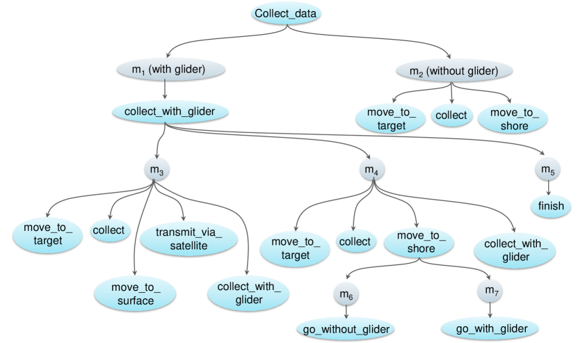
Figure 4: HTN model for the domain of marine environments. Gray nodes $m_{1},\ldots,m_{7}$ represent methods and blue nodes represent primitive and compound tasks.

Going back to the planning decisions, if the planning agent chooses the option that the diver should do a solo dive without the glider, the solution would be different than if the choice is to go with the glider. That is, if the planning agent chooses the other way, it faces another planning decision, i.e., the choice between methods $m_{3}$ and $m_{4}$, where each decision would eventually lead to a different plan. Now assume that we want to solve the problem where we have different gliders that can accompany the diver, where these gliders have different amounts of available power. The choice of which glider to accompany the diver, that is, the binding of the glider variable to a specific glider, may also affect the computed plan. Imagine now that the tasks in $m_{4}$’s task network are all compound and unordered. If the planning agent chooses the task move_to_shore to decompose first, this will lead eventually to executing one of the operators go_without_glider and go_with_glider, which in turn, affects the applicability of other methods and operators. This might lead eventually to a plan that might be different than choosing to decompose the move_to_target task first.

Bringing risk into perspective by having risk-inducing operators in HTN planning requires risk evaluation in each planning choice when solving the HTN planning problems.

Say now the driver needs 10 minutes for sure to return to the shore with the glider. However, when the diver dives back by himself, it will take him 2 minutes to reach the shore with a probability of 80%, and 20 minutes with a probability of 20%. Thus, going alone involves more risk than going with the glider. The existence of these two risk-inducing actions characterises the choice between methods $m_{6}$ and $m_{7}$ as risk involving. This makes, in turn, the choice between $m_{4}$ and $m_{3}$ risk involving, too. Similar reasoning can be applied to choices of bindings and task decompositions.

5.2 Risk Awareness

The choices made during planning eventually influence the outcome of the planning process, that is, the plans. If the quality of plans is not important, these choices can be done non-deterministically. However, rational decision makers aim at maximising their expected utility (see Section 2). Applying this approach to HTN planning with risk, the aim is to maximise the expected utility of the resulting plan.

Since each planning decision eventually contributes to the quality of the solution, maximising the expected utility of the solution means that the planning agent should evaluate the expected utility obtained from each planning decision. To enable this, we employ utility functions that expresses the risk attitude required to solve a planning problem. The utility function is assigned to the planning agent and used to express its preferences over the different outcomes of operators. This enables computing the expected utilities of the operators. Then, the general process should be evident: these expected utilities are propagated to methods to allow making informed choices that maximise the expected utility of the final plan.

Definition 5.1 (Risk-aware HTN Planning).

A risk-aware HTN planning problem is a 4-tuple $P_{r}=\langle s_{0},tn_{0},D,U\rangle$, where $s_{0}$ is the initial state, $tn_{0}$ is the initial task network, $D=\langle O,M\rangle$ is a risk-involving planning domain consisting of cost-variable operators $O$ and a set of methods $M$, and $U$ is a utility function that expresses a certain attitude $ATT$ by evaluating the operator costs. A plan $\pi$ is a solution to $P_{r}$ if and only if $\pi$ has a maximum expected utility $EU(\pi)$ that reflects the chosen attitude $ATT$.

Definition 5.2 (Risk-aware HTN planning Agent).

A risk-aware HTN planning agent is an HTN planning agent that solves risk-aware HTN planning problems $P_{r}$ and behaves by adopting the attitude $ATT$ defined in the planning problem.

5.3 Risk Attitudes

Risk-aware HTN planning agents can show various attitudes towards risk in different situations. We categorise risk-aware HTN planning agents following the taxonomy presented in Section 2. The first category includes planning agents with a static risk attitude, and the second one consists of agents with a dynamic risk attitude. These two categories differ in the type of utility functions that planning agents use and also in the way they evaluate the expected utility of individual planning choices. While the planning agent with a static risk attitude accounts only for the increase/decrease in the resource consumption (not in the amount of resource itself) when making planning decisions, the planning agent with a dynamic risk attitude makes planning decisions while considering the amount of the resource itself.

5.3.1 Static Risk Attitudes

Agent’s static attitude does not change during planning. It is given in advance (e.g., encoded by a domain expert) and can be selected based on the degree of the risk tolerance required for each planning problem.

For agents with static risk attitudes, we assume there are unlimited resources, i.e., there is no limit on how much operators can consume. However, agents should act rationally by making choices that contribute to the maximisation of the plan’s expected utility.

We now define a family of utility functions that can express a static risk attitude of risk-aware HTN planning agents. This family includes linear and exponential functions that are commonly used to express risk-sensitivity [42, 43, 44]. We denote this family by $U_{c}$.

$\forall v_{tp}\in V_{TP}$, such that $v_{tp}=o=\langle pt(o),pre(o),\mathit{eff(o)},c(o)\rangle$ and $c(o)=\langle(p_{1}(o),c_{1}(o)),(p_{2}(o),c_{2}(o)),\cdots,(p_{n}(o),c_{n}(o))\rangle$ and $i\in[1,n]$:

$$U_{c}(c_{i}(o))=\begin{cases}c_{i}(o),&\text{if neutral};\\ \\ \frac{a(e^{a\alpha c_{i}(o)}-1)}{\alpha},&\text{otherwise},\end{cases}$$ (1)

where:

• $a$ is an attitude-determinant coefficient, and

• $\alpha$ is a curving coefficient driving the shape of the utility function.

When the attitude-determinant coefficient $a$ is positive ($a>0$), the utility function is used to express a risk-seeking attitude, while when it is negative ($a<0$), the utility function expresses a risk-averse attitude. Also, using the curving coefficient $\alpha$, we can express a whole spectrum of risk-sensitive attitude such that the bigger $\alpha$ is, the more risk-sensitive the agent is. For $a>0$, the $\alpha$ parameter allows to express a whole range of risk-seeking attitudes from being extremely risk-seeking such that the agent assumes that nature makes the outcomes as much suited for the agent as possible, to the least degree of risk-seeking attitude. Similarly, when $a<0$, using $\alpha$, we can express a whole spectrum of risk-averse attitude, from being extremely risk-averse such that the agent assumes that nature plays against it and it hurts as much as it can, to being at the least degree of risk averse. 

Figure 5(a) and Figure 5(b) show examples of the exponential utility functions with varying values of $\alpha$ for both the risk-seeking and the risk-averse attitudes, respectively. We see that in the utility function of the risk-seeking attitude, the utility decreases for bigger operator costs but at a slower rate, i.e., the slope of the function decreases, which makes large operator costs look smaller and makes the planning agents that adopt this attitude willing to choose methods that have a high risk if it has a possibility of upside potential, i.e., the possibility of leading to small operator costs. On the other hand, we see that the utility function for the risk-averse attitude has a downward concave curve, where the concavity increases dramatically for large operator costs (the slope increases). This gives an exaggerated negative weight to the possible large operator costs. This kind of utility function allows a risk-averse planning agent to follow an avoidance strategy by shying away from method choices that would expose it to possible large operator costs, even if such method have the possibility of upside potential, i.e., the possibility of leading to operators with possible small costs.

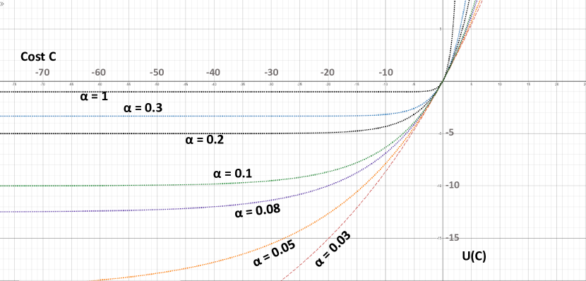
(a) Utility functions of risk-seeking attitudes.

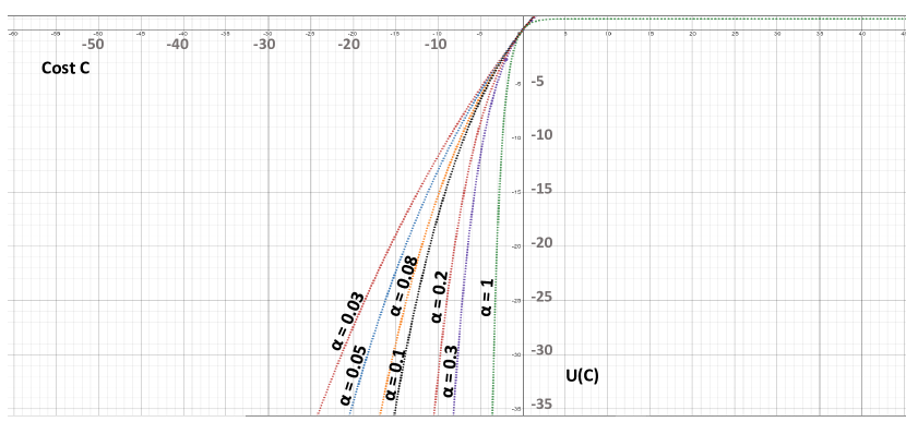
(b) Utility functions of risk-averse attitudes.

Figure 5: An illustration of an exponential utility function for the risk-seeking (a) and risk-averse (b) attitudes with varying values of the parameter $\alpha$.

5.3.2 Dynamic Risk Attitudes

An Agent’s risk attitude is dynamic if it changes during planning. How it changes can, for example, depend on the amount of resources the agent has. A resource is an object that has a limited capacity $\bar{r}$ for use by operators. Thus, we define a resource $R$ as a positive real value ($R>0$). . For example, in marine environments A.3, the resource can be the on-board energy/power that the glider’s battery has, the amount of air that the glider has, the time of the mission, or any combination of them. We consider resources that are disposable/consumables – a type of resources that can be used a limited number of times until they are fully exhausted.  Each time an operator is executed, the resource is decreased by an amount equivalent to the operator’s cost. For example, the energy held in the glider’s batteries decreases each time an operator executes an action.

Having a utility function that expresses a dynamic risk attitude allows a risk-aware HTN planning agent to switch its risk attitude depending on the available amount of resources. To that end, we use the definition of a one-switch utility function, which supports a single switch of the risk attitude. We denote the family of utility functions that model a dynamic risk attitude as $U_{d}$.

$\forall v_{tp}\in V_{TP}$, such that $v_{tp}=o=\langle pt(o),pre(o),\mathit{eff(o)},c(o)\rangle$ and $c(o)=\langle(p_{1}(o),c_{1}(o)),(p_{2}(o),c_{2}(o)),\cdots,(p_{n}(o),c_{n}(o))\rangle$ and $i\in[1,n]$:

$$U_{d}(R+c_{j}(o_{i}))=R+\mathscrsfs{D}\ (\frac{1-e^{-\alpha(R+c_{j}(o_{i}))}}{\alpha})$$ (2)

where the parameter $\mathscrsfs{D}>0$ determines the trade-off between the risk-aversion and the risk-neutrality, $\alpha$ also determines the degree of risk-aversion, and $R$ is the remaining amount of the resource.

Figure 6 shows examples of the one-switch utility function with varying values for the parameter $\mathscrsfs{D}$ and a constant $\alpha$ value of 0.04. Since we are discussing HTN planning in cost-based domains, the resource in HTN planning will decrease after each execution of an operator. In this case, the attitude of an HTN planning agent can change from being risk-neutral to being risk-averse after a certain threshold.

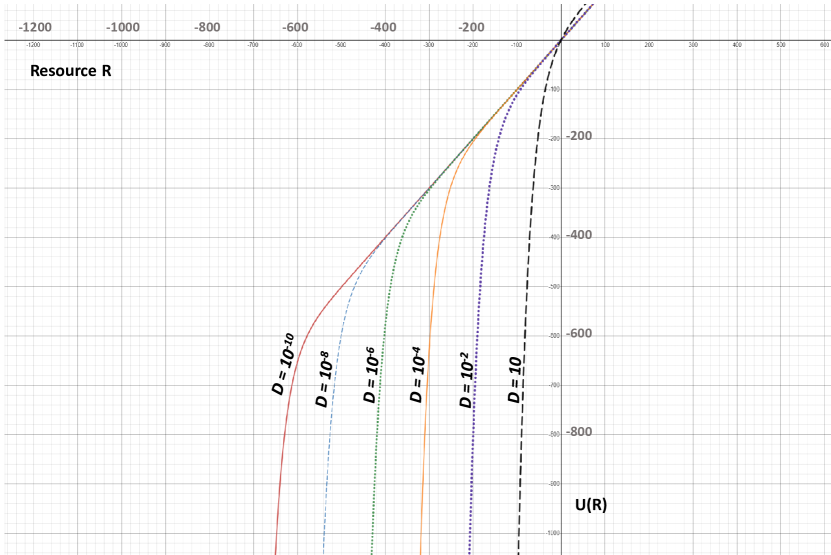
Figure 6: One-switch utility function with varying constant value $\mathscrsfs{D}$, which controls the trade-off between risk-neutrality and risk-aversion. The utility function is risk averse for very low resource and switches to a risk-neutral attitude after a threshold. All illustrated cases have $\alpha=0.04$.

As we shall see in Section 8, after introducing the knowledge necessary to understand the modelling of dynamic risk attitude, the evaluation of outcomes and the propagation of the evaluation to higher hierarchical levels following the dynamic risk attitude appears to be complicated.

5.4 Plan’s Expected Utility

The ultimate objective when solving risk-aware HTN planning problems is to find optimal plans that follow a specific risk attitude. So, plan optimality here entails plans with highest expected utilities. The definition of plan’s expected utility affects the approach followed to solve risk-aware HTN planning problems. Therefore, we provide several definitions for plan’s expected utility by exploring and utilising relevant definitions from the AI planning literature.

One way to define expected utility of plans is by combining expected utilities of some other smaller parts of the planning problem, such as actions or groups of actions. In particular, classical planning problems are divided into subproblems each of which is solved separately and the results are combined into plans [45]. More specifically, a plan consists of multiple segments such that each segment has an action, or course of actions in the general case, with possible states (effects of the actions) with their corresponding costs, as illustrated in Figure 7. Since actions have a probability distribution over possible action effects with their corresponding costs, each segment also contains a probability of distribution over possible states and corresponding action costs. So, we could compute the expected utility of such plans using the following equation.

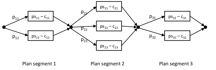
Figure 7: A plan consisting of three segments. Each segment $i$ contains the probability distribution over possible states and the corresponding action cost, i.e., resource consumption in a particular state. $p_{ij}$ denotes the probability of having state number $ps_{ij}$ in plan segment $i$ with the corresponding resource consumption of $c_{ij}$. Adapted from [45].

$$E(u(\pi))=\sum_{i=1}^{2}\sum_{j=1}^{3}\sum_{k=1}^{2}[p_{1i}p_{2j}p_{3k}u(c_{1i}+c_{2j}+c_{3k})]$$ (3)

where: $c_{1i}$, $c_{2j}$, and $c_{3k}$ are the costs of of actions of the first, second, and third segments of the plan, respectively, with their corresponding probabilities $p_{1i}$, $p_{2j}$, and $p_{3k}$.

In the general case and for risk-aware HTN planning problems, the expected utility of a plan $\pi=\langle o_{1},o_{2},\ldots,o_{f}\rangle$ is defined as follows.

$$E(u(\pi))=\sum_{i=1}^{k}\sum_{j=1}^{l}\ldots\sum_{m=1}^{n}[p_{1i}p_{2j}\ldots p_{sm}u(c_{1i}(o_{1})+c_{2j}(o_{2})+\ldots+c_{sm}(o_{f})]$$ (4)

where:

• $s$ is the number of plan’s segments

• $k$, $l$, $\ldots$, $n$ are the numbers of possible effects/costs for the first, second, $\ldots$, and last operator

• $c_{1i}$, $c_{2j}$, $\ldots$, $c_{sm}$ are the costs of operators in the first, second, $\ldots$, sth segments

• $p_{1i}$, $p_{2j}$, $\ldots$, $p_{sm}$ are the corresponding probability of operators in the first, second, $\ldots$, sth segments

• $u(c_{1i}(o_{1})+c_{2j}(o_{2})+\ldots+c_{sm}(o_{f}))$ is the utility of all plan’s trajectories defined using a utility function of the risk-aware HTN planning agent

However, we can also maximise the expected utility of operators within each segment and then multiply the results. The only restriction here is that the used utility functions must enable segmentation. For example, the family of concave and convex exponential utility functions and linear utility functions can be used. For example, for exponential utility functions, the calculation of the expected utility can be segmented as follows.

$$\begin{split}E(u(\pi))&=\sum_{i=1}^{k}\sum_{j=1}^{l}\ldots\sum_{m=1}^{n}[p_{1i}p_{2j}\ldots p_{sm}\dfrac{ae^{\alpha(c_{1i}(o_{1})+c_{2j}(o_{2})+\ldots+c_{sm}(o_{f}))}}{\alpha}]\\ &=\sum_{i=1}^{k}[p_{1i}\dfrac{ae^{\alpha c_{1i}(o_{1})}}{\alpha}]\times\sum_{j=1}^{l}[p_{2j}\dfrac{ae^{\alpha c_{2j}(o_{2})}}{\alpha}]\times\ldots\sum_{m=1}^{n}[p_{sm}\dfrac{ae^{\alpha c_{sm}(o_{f})}}{\alpha}]\\ &=EU(o_{1})\times EU(o_{2})\times\ldots EU(o_{f})\end{split}$$ (5)

where: $EU(o_{1})$, $EU(o_{2})$, $\ldots$, $EU(o_{f})$ are the expected utilities of the plan’s operators.

In this case, the expected utility of each operator or set of operators can be maximised separately and the result can be combined by multiplying the individual maximised expected utilities.

Another way to define the expected utility of plans is by using probabilities of success and utilities of actions [46]. The assumption here is that each action has a probability of success and a utility. Then, the expected utility of a plan is a multiplication of two products. The first one is the success probability of all successful actions, such that the success probability of each action is either independent or it depends on some of the successful actions that were previously executed in the plan. The second product is the product of the utilities of all successfully executed utilities.

For risk-aware HTN planning, the expected utility of a plan $\pi=\langle o_{1},\\ o_{2},\ldots,o_{k}\rangle$ can be defined as follows.

$$E(u(\pi))=\prod_{i=1}^{k}p(r_{i}|r_{1}^{i-1}=1,\pi)\prod_{i=1}^{k}u(o_{i};r_{i}=1)$$ (6)

where $p(r_{i}|r_{1}^{i-1}=1,\pi)$ is the probability of a successful execution of operator $o_{i}$ ($r_{i}=1$) in the plan $\pi$. This probability depends on some of the previously executed operators $r_{1}^{i-1}=1$. $u(a_{i};r_{i}=1)$ denotes the utility of an operator $o_{i}$ if it executes successfully $r_{i}=1$. The utility of a failure is 0.

Equation 6 restricts the effects of operators to binary values; failure and success, where the utility of failure is 0. Thus, in order to adapt this equation to compute expected utility of plans for risk-aware HTN planning problems, restrictive assumptions of the possible operator effects and utility computation should be made. In particular, operators can have either successful or unsuccessful effects. Moreover, since the utility of unsuccessful operators is 0, operator utilities are only computed for the successful outcomes (effects) with a single cost. Our framework is more general and allows operators with multiple possible costs and effects.

The last possibility defines the expected utility of a plan trajectory, which is a possible sequence of operators. This is done by using operators with a probability distribution over effects and utilities of each state resulting from the execution of the operator, i.e., possible effects. More specifically, the expected utility of a plan trajectory is defined as follows [47]. 

$$E(u(\pi_{k}))=\sum_{i=1}^{n}p(o_{i})\times u(c_{ij}(o_{i}))$$ (7)

where: $k$ is the number of the trajectory among all possible plan’s trajectories and $c_{ij}(o_{i})$ is the cost of one of the possible outcomes of operator $o_{i}$ in the trajectory.

6 On Solving Risk-Aware HTN Planning Problems

All the ingredients necessary to define specific risk-aware HTN planning problems and develop approaches that can solve them have been presented thus far. Next, we discuss aspects and possibilities of solving HTN planning problems using simple settings of our framework as specific solutions for given domains will need to be tailored to those domains, their requirements, and specific risk properties. We assume actions have one effect with a probability distribution over possible costs. We consider agents with a static risk attitude. To compute the expected utility of plans, we adopt Equation 4 and we restrict the utility functions to the linear and exponential utility function as defined in Equation 1 to allow plans segmentation as exemplified in Equation 5.

While we do adopt simplifications, we go beyond providing a discussion for state-based HTN planning only. That is, we also explore some possibilities within plan-based HTN planning. We refer to the former model as risk-aware state-based HTN planning, and to the latter model as risk-aware plan-based HTN planning. For each model, we consider two cases. In the first case, we use the utility functions illustrated in Equation 1 and any linear transformation of them. We shall see that some approaches that can find cost-optimal plans in both models can be adapted to find plans with the highest expected utility if the expected utility of the plan is defined according to Equation 4. The main reason is that the computation of the expected utility can be divided into segments.

In the second case, we discuss the usage of utility functions that do not allow segmentation, i.e., utility functions other than the family of utility functions from Equation 1. Then, finding the plan with the highest expected utility, as defined in Equation 4, is more complex as it can require the enumeration of all plan trajectories, in the worst case. This case will be discussed in Section 8.

6.1 Risk-Aware State-Based HTN Planning

In state-based HTN planning, the current state of the world is tracked at each planning step. Having the state at hand at each planning step is useful to solve risk-aware state-based HTN planning for two reasons. First, we can adapt existing approaches that use state-based heuristics to guide HTN planning towards cost-optimal plans to solve risk-aware state-based HTN planning problems. Second, tracking the state during planning allows extending our work to planning agents that can express their preferences over the state of the world. For example, being in a particular state can make a risk-averse agent to have a utility different from the utility of a risk-seeking agent.

Heuristics are a popular concept in AI planning for searching for the desired outcome in large search spaces. Heuristics-based HTN planning approaches appear to be relevant for constructing approaches for solving risk-aware HTN planning problems. In the scope of state-based HTN planning, one can adopt a generic method for guiding the search process by using an arbitrary classical heuristic [48, 49]. The method is based on relaxing the HTN planning problem into a classical planning problem, which is used to calculate the heuristics. The relaxed model contains two types of actions: actions that are converted from HTN methods $A_{M}$ and the original actions that exists in the HTN problem $A$. The heuristics calculated in the relaxed model estimate the number of steps needed to reach the goal, i.e., the sum of decompositions and actions needed to reach the goal for each node.

The relaxed model can be used to create admissible heuristics for state-based HTN planning, which can then be used to find optimal plans. This is exactly the feature that makes the present approach suitable also for solving state-based risk-aware HTN planning problems. In particular, it has been suggested that an admissible heuristic could be computed by introducing action costs in the relaxed model, where all converted actions $A_{M}$ could be given a zero cost, while the original actions $A$ could be given an arbitrary positive costs [48]. Then, we could find optimal plans by employing the A* algorithm in combination with an admissible classical heuristic (e.g., LM-cut [50]) for the relaxed model [51].

We propose to solve the risk-aware state-based HTN planning problem as a maximisation problem using Algorithm 1. The algorithm uses A* to search for plans and takes as an input the fringe, which represents all search nodes $n$ explored together with the value that A* uses to order these nodes in the fringe, and the domain description $D$, and the problem description $P$. The value that A* uses represents an estimation of the expected utility of the plan that can result after decomposing the task network of $n$. It is computed for each search node $n$ as the sum of two values: the first one is the sum of the expected utilities of all operators that are added to the plan so far $sum(n^{\prime}.\pi)$; the second one is an admissible heuristic that estimates the expected utility of plan segments computed by the relaxed model to guide the search in state-based HTN planning by computeRCAdHeur in Algorithm 2). The heuristic should be computed on the relaxed model after setting the cost of method actions $A_{M}$ to zero, and assigning the original actions $A$ a cost equal to the expected utilities of the corresponding operators in the domain description (lines 5 and 6 in Algorithm 2). The expected utility of an operator is computed as the weighted average of the utilities of each possible cost of the operator. The weights represent the probability distribution of these costs.

At the beginning of Algorithm 1, the fringe contains an initial node that consists of the initial state, initial task network, and an empty plan. An admissible heuristic is then computed (line 2) and the node is added to the fringe. The algorithm keeps looping to process all the nodes in the fringe until the fringe is empty. At each iteration, a test is made on whether a plan is created, i.e., all tasks in the node’s task network are primitive tasks and the node’s plan is applicable at the initial state and can accomplish the initial task network (lines 7 and 8). If this is the case, the plan is returned. Otherwise, the set of all tasks that do not have predecessors in the node’s task network are returned (line 9). For each of these returned tasks, if the task is primitive, it is applied and added to the node’s plan (line 12). Then, the heuristic of the node is computed again and the node is added to the fringe according to its annotated value (lines 13 and 14). If the task is compound, for all methods that can decompose it and are applicable, a new search node is generated, which equals to the current search node, but with replacing the compound task in the search node’s task network by the tasks in the method’s task network. After that, the node is added to the fringe in its right order after computing its value (lines 18 and 19).

Algorithm 1 FindPlans

1:$n_{init}$ $\leftarrow$ ($s_{0}$, $tn_{1}$, $\phi$)

2:$n_{init}$.heuristic $\leftarrow$ computeRCAdHeur($n_{init}$ ,D, P)

3:fringe $\leftarrow$ { $n_{init}$ }

4:function FindPlans(fringe, D, P)

5:     while fringe $\neq\phi$  do

6:         $n\leftarrow$ fringe.first()

7:         if $\forall$ t $\in$ n.tn : isPrimitive(t) $\land$ applicable(n.$\pi$, n.$s_{0}$)  then

8:              return n.$\pi$          

9:         U $\leftarrow$ findUnconstrainedTasks(n.tn)

10:         for all t $\in$ U do

11:              if isPrimitive(t) $\land$ $\exists$ o $\in$ D.O: pt(o) = t $\land$ pre(o) $\subseteq$ n.s  then

12:                  n’ $\leftarrow$ n.apply(t)

13:                  n’.heuristic $\leftarrow$ sum(n’.$\pi$)+computeRCAdHeur(n’,D,P)

14:                  fringe.addAndOrder(n’)

15:              else

16:                  for all m $\in$ D.M :ct(m) =t $\land$ pre(m) $\subseteq$ n.s do

17:                       n’ $\leftarrow$ n.decompose(t,m)

18:                       n’.heuristic $\leftarrow$ sum(n’.$\pi$)+computeRCAdHeur(n’,D,P)

19:                       fringe.addAndOrder(n’)                                               

20:     return Failure

Algorithm 2 computeRCAdHeur

1:function computeRCAdHeur(n, D, P)

2:     RC $\leftarrow$ buildRCModel(n, P)

3:     for all $A_{m}$ $\in$ RC do

4:         $A_{m}$.setCost(0)      

5:     for all $A$ $\in$ RC : $\exists$ o $\in$ D.O $\land$ pt(o) = A do

6:         $A$.setCost(ComputeExpectedUtility(P.utilityFunction, o))      

7:     AdmissableH $\leftarrow$ computeH(RC)

8:     return AdmissableH

6.2 Risk-Aware Plan-Based HTN Planning

Also in the case of risk-aware plan-based HTN planning, we resort to a heuristic approach and turn to A* [15]. The heuristic is computed on a TDG similar to the one defined in Definition 4.1. However, unlike our definition of TDG, which is a representation of parametrised domain models, the TDG from [52] is a representation of ground domain models, i.e., variable-free models. Moreover, since this approach focuses on plan-based HTN planning, method nodes in the TDG represent partial plans, i.e., the whole task network resulting from decomposing a specific task using this method. Now, the feature of this approach relevant to our treatment is that primitive tasks are assigned non-negative costs while methods and tasks get cost estimates by preprocessing the ground domain model. More specifically, in the preprocessing step, the TDG is computed so that method and tasks vertices are assigned costs estimates in a bottom up manner. The cost of a method vertex is the sum of all cost estimations of tasks in its task network, whereas the cost of a task vertex is the minimum cost among all estimated costs of methods that can decompose it. Then, during search, the cost estimation, i.e., the heuristic, of each partial plan is computed by summing up the precomputed cost estimations for the tasks that are part of the plan, while also taking the minimum of the cost estimation among the groundings of a particular task.

We adapt the approach of by Bercher et al. [15] by incorporating utility functions to guide the A* algorithm to solve risk-aware plan-based HTN planning problems. This means that the new heuristic will estimate expected utilities of methods and tasks. However, this new heuristic should be also admissible in order for the algorithm to compute the plan with the highest expected utility. The expected utility estimations and the search are based on a ground model of the CV-TDG (Section 4.3), where the graph nodes represent instantiations of the parametrised tasks and methods instead according to the problem instance.

There is also a preprocessing step in which we compute the expected utilities of primitive tasks. These expected utilities are defined and computed according to utility theory as the weighted average of the utilities of each the possible costs of primitive tasks. The weights represent the probability distribution of these costs. Thus, $\forall v_{tp}\in V_{TP}$, such that $v_{tp}=o=\langle pt(o),pre(o),\mathit{eff(o)},c(o)\rangle$ and $c(o)=\langle(p_{1}(o),c_{1}(o)),(p_{2}(o),c_{2}(o)),\cdots,(p_{n}(o),c_{n}(o))\rangle$ and $i\in[1,n]$, the expected utility of $o$ is defined as follows.

$$EU(o)=\sum_{i=1}^{n}U_{c}(c_{i}(o))*p_{i}(o)$$ (8)

The utility of each outcome $U_{c}(c_{i}(o))$ is computed using one of the utility functions defined in Equation 1, which allows choosing a risk attitude and determining its intensity. Then, as heuristics that determine expected utility of compound tasks and method nodes we use Equations 9 and 10, respectively. For a compound task, the expected utility $EU_{T}(v)$ is the maximum of the expected utilities of all methods that can decompose it. The expected utility of a method is the product of the expected utilities of the tasks in its task network.

$$EU_{T}(v)=\begin{cases}EU(o),&\text{if $v=o$ and $v=v_{tp}$ and $v_{tp}\in V_{TP}$};\\ max_{(v,v_{m})\in E_{TC\to M}}EU_{M}(v_{m}),&\text{if $v=v_{tc}$ and $v_{tc}\in V_{TC}$}.\end{cases}$$ (9)

$$EU_{M}(v_{m})=-\prod_{(v_{m},v_{tc})\in E_{M\to TC}}|EU_{T}(v)|$$ (10)

In the searching step, for each partial plan, we retrieve the maximum expected utility of a compatible grounding of each task $comp(t(\bar{\tau}))$. Then, the heuristic that computes the expected utility of this partial plan is the product of the the expected utilities of all its compound tasks as shown in Equation 11. Partial plans are sorted by A* based on the product of the expected utilities of their compound tasks multiplied with the product of expected utilities of their primitive tasks. The first product represents an overestimation of the expected utility gained from decomposing the set of the compound tasks into primitive tasks, whereas the second product represents the expected utilities of the already refined tasks, that is, the expected utility of the primitive tasks resulting from all previous refinements. Sorting partial plans in A* according to their expected utility provides the approach with the ability to implicitly make informed choices of methods when decomposing a compound task. These informed choices are made based on the expected utility of the partial plan resulting from this decomposition.

$$EU_{TDG}(P)=-\prod_{l:t(\bar{\tau})\in P\land t(\bar{\tau})compound}|(max_{v_{tc}\in comp(t(\bar{\tau}))}EU_{T}(v_{tc}))|$$ (11)

Since the heuristic considers the maximum expected utility as an estimation for each compound task and considers the maximum expected utility among all compatible groundings, according to the definition of admissibility of maximisation problems (see Definition 2 in [53]), the heuristic is admissible and can be used to guide the search to compute the plans with the highest expected utility.

Recall that the variable costs of operators are strictly negative. Then, the utility of these costs will have a strictly negative value according to Equation 1 (see Figures 5(a) and 5(b)). This means that the expected utility computed by Equation 8 is also strictly negative. Thus, we take the absolute values of the expected utility of operators when computing the heuristic. Furthermore, when computing the estimation of a method node, we take the absolute value of the expected utility estimation of the tasks in this method’s task network, but we multiply the final product by -1, as shown in Equation 10. We do so to ensure that the product is not affected by the sign of the utility and that the estimation of the expected utility of compound task nodes is always chosen to be the least-negative estimated expected utility of all methods that can decompose it. The same argument holds when computing the expected utility of a partial plan. According to Equation 11, the resulting plan has the maximum expected utility with respect to the definition of the expected utility given in Equation 5, but with absolute values of the expected utility of the plan’s constituent operators.

$$E(u(\pi))=-|EU(o_{1})|\times|EU(o_{2})|\times\ldots\times|EU(o_{f})|$$ (12)

7 Related Work

Risk and especially uncertainty have been the concern of several works on AI planning. We overview both non-hierarchical AI planning and HTN planning approaches. We start by briefly summarising works that solve planning problems under uncertainty followed by reviewing works that incorporate utilities, risk, and/or risk attitudes. Then, we review works that study HTN or HTN-like planning under uncertainty followed by an overview of studies that incorporate some form of utilities and risks in HTN or HTN-like planning. Finally, we discuss approaches that use additional information to aid the decision-making process of HTN planning.

7.1 Uncertainty in Non-Hierarchical Planning

Planning under uncertainty has already been the object of scientific reviews [54, 55], where uncertainty is usually defined as incomplete or faulty information from the environment, which in turn leads to uncertain initial state and action effects [56].

There are two types of planning under uncertainty, namely contingent planning and conformant planning. Contingent planning deals with the task of generating a conditional plan given uncertainty about the initial state and action effects, but with the ability to observe and sense some aspects of the current world state during execution, partially or fully [57, 58]. Conditional plans are plans that have some branches executed conditionally based on the outcome of sensory actions [59]. Conformant planning is the task of generating plans given uncertainty about the initial state and action effects, but without any sensing capabilities during plan execution (no observability) [60].

Both types of uncertainty about action outcomes is usually expressed logically using conjunctions or numerically using probabilities [61, 62]. In the first case, planning approaches should find plans that are successful regardless of which particular initial world we start from and which action effects occur, e.g., [59, 63, 64]. In the second case, planning approaches aim at finding plans either with the highest probability of succeeding or with a success probability that exceed a certain threshold, e.g., [65, 66, 67].

Most approaches to AI planning do not make clear distinction between risk and uncertainty in action outcomes as defined in decision theory. In particular, with few exceptions that we present in the next section, approaches that model action outcomes probabilistically do not incorporate the notion of risk or deal with risk attitudes of planning agents.

7.2 Risk in Non-Hierarchical Planning

Our approach is closely related to studies that incorporate utilities in planning, such as [68, 69, 70, 71, 44, 45]. However, our approach is different than these approaches in incorporating risks, risk attitudes, and utilities in hierarchical constructs. These studies extend classical planning problems with concepts from utility theory and incorporate some form of utilities in planning, usually assuming a risk-neutral attitude of the planning agent. An interesting approach is presented in [44], where planning problems are characterised by probabilistic effects of actions, actions with costs (resource consumption), and rewards of goal states. Similar to our work, this approach aims at finding plans with the highest expected utility for risk-sensitive agents. The agents have utility functions (linear or exponential) that are used to quantify their preferences, in terms of utility, over the outcomes. Moreover, utility functions have been incorporated in uncertain robot navigation domains to demonstrate how utility functions can be used to model given risk attitudes and soft deadlines [45]. The uncertainty in this domain results in actions with varying execution times, i.e., costs, and a totally-known probability distribution. The paper discusses the incorporation of risks by using exponential utility functions to evaluate outcomes and find plans with the highest expected utility.

7.3 Uncertainty in HTN Planning

A form of uncertainty has also been considered in HTN planning. In [72], two types of uncertainty are defined. The first type entails having partial observability of the state, which is represented as a probability distribution over belief states. The second type of uncertainty is represented as a probability distribution over action effects. This corresponds to our definition of risk. The aim is to find plans with the highest probability of success, which is different than ours. This work does not consider action costs nor does it study risk attitudes.

A more recent work formalises fully observable non-deterministic HTN planning problems where actions have multiple effects [73]. While this work introduces solution criteria for solving these problems, it does not consider plan quality, action costs, or risk attitudes. Another recent work solves navigation planning problems in marine environments, which have a high degree of uncertainty [14]. In this domain, navigation actions have uncertain costs due to the uncertainty in flow forecast. Thus, the cost of moving from a location to another is estimated and can be different from the actual cost. This approach aims at finding the plan with the highest probability of having the total cost lower than a user-defined upper bound. Unlike our work, this approach does not consider risk when solving the problem, thus, it cannot find plans with the highest expected utility.

Computing plans that meet certain probability thresholds with respect to the consumption of critical limited resources has been the focus of the work of Biundo et al. [13]. The uncertainty is modelled for continuous resources as a continuous probability distribution associated with operator to indicate the resource consumption of a specific operator. This information is then propagated to the higher levels of task hierarchy to help taking informed choices. Since the probability distribution of operator costs is not totally known, the model of operator costs correspond to uncertainty-inducing actions. The goal of this approach is to compute heuristics to guide the planning process to compute plans that do not exceed a certain threshold of resource consumption.

Some works adopt hybrid planning approaches in the sense that HTNs are used to guide solving non-hierarchical planning problems or HTN planning is combined with other planning techniques to solve planning problems in uncertain domains. In [74], probabilistic HTNs are used for planning in Markov Decision Processes (MDP) environments such that uncertainty is represented by probabilities that encode the subjective knowledge of users on how likely a specific method is chosen to decompose a compound task. In MDP environments, utilities are assigned to states in the form of rewards and the objective is to find the plan with the highest expected utility. Another approach uses HTNs to restrict its search for plans using fully observable non-deterministic non-hierarchical planning techniques [75]. Actions in HTNs are extended to model multiple non-deterministic effects. Similar to this approach are the works presented in [76] and [77], which consider non-deterministic effects of actions without defined probabilities but use HTNs to guide the search of the underlying non-hierarchical planning techniques. All presented approaches for hybrid planning do not consider uncertainty or risk with respect to action costs, nor do they consider agent’s attitudes. In addition, the last three works do not consider the quality of a solution, but simply the identification of a solution, if available.

7.4 Risk in HTN Planning and HTN-Like Planning

Actions with hard-coded utilities that are not related to action costs but are based on the type of actions and their outcome are considered in [46]. The approach works in robotics domains, where the action outcome represents a binary value of success or failure, and the utility of actions with a failure outcome is 0. The approach aims at finding the plan with the highest expected utility, where the expected utility is computed as a product of the probability of action success, which can be learned online, and the utility of this action. Our work not only supports the utilities and probabilities as defined in this work, but also abstracts away from a specific domain and provides an HTN planning framework that incorporates risk and risk attitudes to solve problems in uncertain and risky domains.

A utility function is used to evaluate the execution cost or effect of primitive tasks in [78]. This approach produces only the least-cost plan and does not deal with risk and risk attitudes in HTN planning. HTN planning was extended to account for stochastic actions that have a probability distribution over multiple action effects [47]. The approach aims at maximising the expected utility, which is computed based on the probability distribution of each action in the plan and the utility. The utility in this work is a reward function that describes the reward obtained from transitioning from one state to another. Similarly, this work does not consider risks and risk attitudes.

An emotional-based planner incorporates expected utilities in a planning formalism similar to HTN planning [79]. Uncertainty is defined and modelled using conditional and probabilistic effects of actions. Since the probability distribution is given, this definition of uncertainty corresponds to our definition of risk. The aim of the planner is to compute plans with the highest expected utility, where expected utilities are computed for actions and are measured in terms of the intensity of the emotions, drives and other motivations it may elicit. The expected utilities are propagated in a preprocessing step to higher hierarchical levels to help make informed choices during planning. Our work is more general and can be used to include the modeling of Macedo et al.. In fact, our work is not only more general but it also builds upon the standard HTN planning formalism, whereas the emotional-based planner works on concepts different than HTN planning ones (cf. cases of plans or abstract plans instead of methods). Moreover, the work of Macedo et al. does not discuss the involvement of risks and risk attitudes in their approach.

Similar to the previous work is the decision-theoretic planner where a different way to abstract conditional probabilistic actions. The system is called DRIPS [80]. The aim is to compute plans with the highest expected utility, where risk and risk attitudes are not taken into account.

7.5 Informed Decision-Making in HTN Planning

Our work can be seen as related to approaches that use additional information in HTN planning to compute quality plans. Such additional information takes the form of heuristics, preferences, and advice. There is also a branch of approaches that order HTN methods using a heuristic function that defines the distance between the goal state of the given planning problem and the goal states of methods [81, 82, 83]. The latter approaches usually aim at improving the planning performance regardless of the resulting plan quality and agent attitudes, and are, therefore, out of scope here.

7.5.1 Heuristics

Heuristics are strategies for deciding which alternatives promise to be more effective to achieve some objective. Heuristics are a popular concept in AI planning used to speed up the planning process and compute optimal plans. Heuristics are also used in HTN planning to guide the computation of optimal plans in mainly deterministic models of domains. An admissible heuristic to find optimal solutions in terms of plan cost in HTN planning was recently proposed in [15]. Minimising the plan cost corresponds to the simplified objective of risk-neutral agents. Similarly, another approach uses a heuristic function to sort unexplored plans based on the sum of an estimated number of steps to reach the current partial plan and estimated number of steps needed to reach the goal [16].

The SHOP2 planner has been enhanced with a limited branch-and-bound optimisation to guide the task decomposition to the cost-optimal plan with a possibly chosen execution time limit [84]. Another approach also uses a branch-and-bound algorithm with an admissible heuristic to guide the search to compute cost-optimal plans and a non-admissible heuristic to search faster [85].

HTN planning is translated into classical planning to compute heuristics that are then used to guide searching for plans [48, 49]. These heuristics estimate the number of decompositions and number of actions required to accomplish a given objective. The approach can be adapted to solve cost-optimal plans. In particular, if an admissible heuristic that enables the computation of optimal-cost plans is used in the relaxed classical planning model, then it can be used to compute cost-optimal plans in the HTN model. Another study translates HTN planning into propositional logic, where optimal plans are defined in terms of their length [51].

Another approach requires users to annotate abstract tasks with lower and upper bounds on the costs of the possible plans that these tasks can be used for [86, 87]. These values are used to speed up the search towards cost-optimal plans. Unlike this approach, we do not require any additional domain-specific information to be encoded. Also this approach follows only the risk-neutral attitude.

User ratings and social trust are employed as an indicator for choosing preferable methods when composing Web services in [88]. In this specific domain, user ratings and social trust can be seen as different attitudes toward some social phenomenon. Our work abstracts away such specificities by proposing a general framework that allows incorporating attitudes and accounting for risks and/or uncertainty in HTN planning for any domain.

Although the presented approaches operate in deterministic domains, since they are based on averaging costs out to compute cost-optimal plans, they all can be adapted to domains with risk-inducing actions. However, the attitude that they follow correspond only to a risk-neutral attitude.

7.5.2 Preferences and Advice

Since risk attitudes represent a common type of preference structure, it comes naturally to also look at works that incorporate any other form of preferences in HTN planning. A line of works focuses on the extension of PDDL3, which is a version of the a Plan Domain Description Language (PDDL) that supports temporally extended preferences and hard constraints [89], with HTNs to find preferred plans [90, 91, 92]. The plans are computed according to encoded preferences over occurrence, decomposition, and instantiation of HTN tasks. The quality of the resulting plans is defined in terms of the number of preference achieved. Theoretically, it might be possible to express risk attitudes using preferences. However, this requires preferences to be provided for each compound task and to be encoded as additional domain knowledge by a planning expert. Our work does not require any additional domain knowledge, nor does it need encodings for compound tasks. Instead, utility functions can be selected automatically based on the required risk attitude or manually by a domain expert. Moreover, encoding the planning choices to comply with a specific risk attitude in form of preferences means that the domain expert should solve the planning problem to know which choices lead to the highest expected utility plan. In addition, existing approaches that use preferences in HTN planning do not deal with action costs in uncertain and/or risk-involving domains.

HTN planning has been extended with hard constraints to model advice on how to decompose methods [93]. These constraints specify limited combinations of expert advice. As in the preference-based HTN planning, these pieces of advice have to be encoded by a domain experts as well as planning experts, and moreover, are not related to attitudes or action costs.

Finally, additional information has been incorporated in the HTN domain knowledge to help make the choice of methods in an informed manner [94]. This is achieved by assigning three values to each method for estimating the performance, cost and probability of success of the respective method. Again, these values depend on the expertise of the domain author and have no association with attitudes and costs of operators in uncertain and/or risky domains as defined in our work.

7.6 Novelty

By reviewing related work in AI planning literature, we note that uncertainty and risk are not conceptually distinguished as provided by decision theory. In particular, planning approaches that model totally known probability distribution over action effects, action costs and states are referred to as uncertainty approaches without consideration of the risk involvement.

Moreover, in most planning approaches, uncertainty forms are expressed in terms of partial observability of states, and uncertainty about action effects or action costs. However, approaches that deal with the latter form of uncertainty usually aim at computing plans with the highest probability of not exceeding a predefined cost limit and do not find plans that comply with a specific attitude.

Risk, on the other hand, is modelled in HTN planning as a hard-coded utility functions that are not related to action costs or a specific risk attitude. On the other hand, approaches that use utilities to evaluate action costs use planning formalisms that deviates from standard HTN planning and do not consider risk and risk attitudes of planning agents.

HTN planning approaches that do some informed guidance of HTN planning towards quality plans are also relevant to our work. Some approaches do consider action costs, but are developed for deterministic domain models and aim at finding cost-optimal plans. Thus, if adapted to domain models with variable costs, they correspond to the risk-neutral attitude. Other approaches use preferences and could be adapted to express attitudes. However, they require encoding the planning choices of risk-sensitive agents by a domain expert.

Thus, we conclude that while there exists a few works that incorporate risk and risk attitudes in non-hierarchical planning, there does not exist an HTN planning approach that models risks involved in action costs and also incorporate utilities in hierarchical constructs to express and guide the planning process according to a particular risk attitude.

8 Discussion

The present work is an initial step towards the study of risk for HTN and AI Planning in general. While we provided a general framework, we identify a number of research questions that sprout from the present investigation.

What kind of challenges might arise when modelling risk-aware HTN planning agent with an arbitrary utility function?

The approaches presented for risk-aware state-based HTN planning and risk-aware plan-based HTN planning assume that the agent has a utility function that belongs to the family of utility functions of Equation 1. What makes this family of utility functions suitable is that it allows maximising different segments of the plan separately. In particular, in the risk-aware state-based HTN planning approach, the value that the A* uses to guide the search is based on summing up the expected utilities of the operators in the plan and the estimated expected utility of the compound tasks to be decomposed. This means that the algorithm is maximising the expected utility of segments of the plan and then combines these segments into one plan. The same reasoning applies to the approach of risk-aware plan-based HTN planning. The decomposition of a task using a specific method might result eventually in a segment of the final plan, which is maximised individually.

The problem becomes more complicated if the agent can have an arbitrary utility function that does not allow segmentation, e.g., $u(c)=(-c)^{3}$. The reason behind this is that, in general, $u(c_{1}\times c_{2})\neq u(c_{1})\times u(c_{2})$. In the worst case, it might be necessary to enumerate all the trajectories of all possible plans to find the one with the highest expected utility. Since this approach is computationally infeasible, to solve such planning problems, while giving flexibility of the choice of utility functions, other planning approaches should be developed.

What challenges are imposed by modelling risk-aware HTN planning agents with a dynamic risk attitude?

When the risk attitude of the agent is static, it is possible to express a whole spectrum of risk attitudes just by changing the curving coefficient in Equation 1. Anyhow, for dynamic risk attitudes, where the risk attitude can change based on, for example, resources or planning history, there might be a need to use utility functions that do not allow segmentation. Consider, for example, the one-switch utility function defined in Equation 2. This utility function can be used to evaluate the operator outcome with respect to the possible remaining resources after executing the operator. However, computing expected utilities of operators and propagating them to higher hierarchical levels is not correct anymore since the utility function does not allow maximising each plan’s segment individually. In this case, it might be necessary to enumerate all possible plan trajectories and compute the utility function for each of them. However, as in the case of static risk attitude, doing an exhaustive search is in general infeasible. Moreover, the remaining amount of resources $R$ is uncertain during planning since operators have variable costs.

Another challenge lies in the necessity for the agent to not only make planning choices that maximise the expected utility but also to account for the possibly limited amount of resources. In fact, limited resources may impede the agent to reach its maximum expected utility if plans are computed assuming unlimited resources.

How can the general framework be specialised?

By modelling different degrees of uncertainty and risk along the wide spectrum of uncertainty. For example, it can be specialised to model uncertainty-inducing actions. In this case, encoding the planning agent’s beliefs about the probabilities of the outcomes is an interesting, yet challenging, research direction that would address further the complexity of real-world domains. Learning the probabilities of outcomes could be a possible direction.

9 Conclusions

In decision theory, risk and uncertainty are usually defined as distinct concepts. We bring such a distinction to the field of planning by considering two types of actions: risk-inducing and uncertainty-inducing actions. We identify the possible sources of uncertainty that have effects on the action outcomes ranging from totally known to totally unknown probability distribution of effects and their corresponding costs. Using this distinction, we developed a general framework for HTN planning that can be specialised by future studies to deal with planning problems that involve risk and uncertainty related to action costs. Since our work is rooted in decision theory, a well-established field of research, we believe that it helps bringing HTN planning a step closer to simulating the way in which decision makers address and solve problems while embracing risk.

We studied a specific realisation of this framework for which actions have single effects and are risk inducing, and planning agents adopt a specific risk attitude, which can be static or dynamic, for making planning choices. We further discussed approaches that can solve such HTN planning problems by incorporating expected utilities with hierarchical constructs to allow finding risk-aware plans, i.e., plans with the highest expected utility that comply with the planning agent’s risk attitude. We also showed that by restricting the type of utility function to the family of linear and exponential utility functions, we can adapt approaches that find cost-optimal plans to solve risk-aware HTN planning problems.

We pointed out that most existing approaches in AI planning do not distinguish between risk and uncertainty in action outcomes, but rather they use uncertainty as an umbrella term even when having risk-inducing actions. Moreover, while some existing approaches incorporate utilities in HTN planning, risk awareness is considered in previous work. We also showed that, in general, planning approaches that guide HTN planning by making informed choices via heuristics or preferences assume deterministic model of the domain and adopt a risk-neutral attitude of planning agents.

Appendix A Real-World Domains with Uncertainty

We look into three case studies derived from real-world domains, namely electric and autonomous vehicles, smart homes, and oceanic environments. These domains are selected because they do exhibit elements of uncertainty and making choices in them can involve risks. For each domain, we illustrate the relevant sources of uncertainty and how each source affects action costs.

A.1 Electric Autonomous Vehicles

Autonomous vehicles are transportation means, typically for humans, that can navigate without or with little human direct control. We illustrate possible sources of uncertainty in the domain of autonomous vehicles when the executing agent is a human and when it is the vehicle.

• Human Agent: When a person is driving a vehicle and is responsible for performing all actions, such as driving, charging the vehicle and changing a lane, the costs of these actions, which can be related to time, money, power or effort, can vary due to multiple internal regular sources, such as the variability in driving skills, habits, tactics, and speed. For example, if the person is driving between two places, it might take him/her an hour or 30 minutes depending on his/her speed. Similarly, the amount of energy consumed and the time spent when moving between two places can vary between different people based on the driving habits and tactics that they have. Also, a sleep-deprived person might fall asleep while driving causing an accident. The consequences caused by driver drowsiness can be statistically studied [95]. Unlike these regular sources, there can also be random internal sources. For example, a driver can have a stroke while driving. Unlike the regular factors that might be predicted by statistically studying the behaviour of drivers, such an event could be hard to predict in advance due to its rareness.

• Autonomous System Agent: If the vehicle is responsible for performing the actions, there can be multiple internal regular sources of uncertainty that affect the variability of action costs. For example, the speed at which the batteries of the vehicle charge and deplete can be uncertain and might change by time depending on the battery life. There are also some random internal sources that lead to unpredictable outcomes. For example, a flat tire will cause the car to stop.

There are also some external, random and regular sources of uncertainty that can affect the variability of costs. For example, a vehicle might fail to perform a charging action if the charging station has a technical problem. This kind of event can be considered random since it is hard to be predicted during planning. Consider another scenario where the vehicle is driving following a planned route and suddenly there is an unexpected road block due to an accident. This random external event might be hard to predict during planning due to its rareness, which in turn makes it hard to know the outcomes of the driving action in advance.

Now let us consider other cases where the external sources of uncertainty are regular. Weather conditions, for example, can be considered as a regular source of uncertainty since they are continuously changing and cannot be determined with certainty. Thus, due to the chaotic character of the atmosphere and the inadequacies in observations and computer models, weather forecasts always contain uncertainties [96]. One way of delivering the weather forecast is using probabilistic forecast in which all forecast elements, such as temperature, wind and precipitation, are probabilistically quantified to express this inherit uncertainty [97]. In the domain of electric autonomous vehicles, the uncertainties in the weather forecasts are reflected on the costs of the driving action. For example, driving between two places in winter can can incur different costs, such as time and power, depending whether it is snowing or not.

Another possible regular external source of uncertainty in this domain is the traffic, which can play a big role in the variability of action costs. Say we want to plan the route between two points using Google Maps, the most used route planning application. Google Maps will show an example of the cost variability due to external regular factors, such as weather conditions and traffic (see Figure 8).

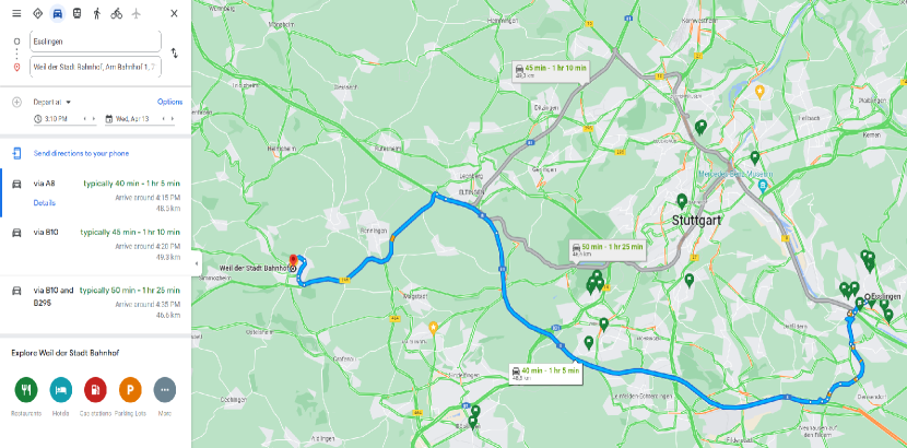
Figure 8: Variability of travelling time in Google Maps [98]

A.2 Smart Homes

Smart homes are those that are aware of their state and that can change such state proactively for the safety, comfort, and needs of its residents [99]. Consider now a family living in a home that is equipped with a system that can coordinate all devices and appliances in the home, and cooperate with a domestic robot similar to the humanoid robot presented in [100]. The robot has multiple sensors and is able to move around the home, pickup and place things, cut and clean for cooking, and clean the floors. As in the previous case study, lets divide between the case of the resident performing the actions and the case of the robot performing the actions.

Imagine a scenario in which the robot is helping a person to cook a meal. Here, we have two types of executing agents; a human and a system (the robot). Let us assume that the robot is mixing the dressing for the meal and the person is chopping some vegetables. The speed in which each of these actions is done is uncertain due to the capabilities of the person and the robot, which are internal regular sources of uncertainty. The probability of the time needed to perform these actions could be measured based on past experience, or it could be partially known during planning. Say that while the person is chopping the vegetables, he gets a knife cut. This leads to a failure in the chopping action and is considered a random internal source of uncertainty since it is an unexpected random event that can lead to consequences hard to quantify in advance during planning.

Consider now a scenario where the robot is cleaning the floor while the inhabitants are moving around, disturbing the robot’s movement. The movement of home inhabitants is an external regular source of uncertainty that can incur different costs, e.g., time and cleanness. Similarly, the robot movement can be considered an external regular source of uncertainty that affects the variability of costs of the inhabitant movement actions. Also, leaving the doors closed by inhabitants is another source of external uncertainty that can affect the action costs of the robot.

A.3 Marine Environments

The exploration of the sea and the collection of samples constitutes what we refer to as “marine environment”. For this we consider two types of agents: scientific divers and underwater gliders, both equipped with a wide variety of sensors to collect ocean environmental data, photos, and videos. During the solo dives of scientific divers, the gliders can be used as drop-in diving buddies to increase the safety of divers by providing them support, such as giving their exact position or carrying an extra air tank [101].

Human behaviour always constitute a big part of uncertainty in most environments due to its variability and unpredictability. This is especially true in extreme environments, such as oceans, that impose high physiological and psychological pressure on people, that is, divers. Intelligence and personality differ between individuals and can have effects on the behaviour underwater [102]. The variability of divers behaviour represents an internal regular source of uncertainty in marine environments, which in turn leads to variability in the costs of actions that are performed. For example, the time needed to take a picture of a specific phenomena under water might differ from one diver to another due to the differences in their behaviours.

When the agents are gliders, i.e., the gliders are responsible for collecting the data, there can be multiple internal regular sources of uncertainty. For example, a malfunction of one of the navigation sensors or the loss of a wing can lead to spending more than expected time and energy to move to the location of interest, or, in the worst case, can lead to complete failure in reaching the location.

A huge part of uncertainty during planning comes from the uncertainty in the flow forecast [14]. This is due to the fact that these systems, like the atmosphere, are chaotic non-linear systems. Thus, flow forecasts in marine environments are considered external regular sources of uncertainty, which leads to cost variability of marine actions, such as navigation and sampling of data, irrespective of whether they are performed by divers or gliders. Another external regular source of uncertainty is due to the quality of the interconnection between the diver and the surface. Since gliders need to communicate with the surface to relocate, the variability of the communication quality can lead to variability in the cost of positioning actions. On the other hand, there also exists many random external sources of uncertainty. For example, an unexpected bio-fouling issue has been reported in the gulf of Mexico where Remora fish—which typically attach to sharks and other large marine animals—held the gliders down until they decided to detach [103]. Another random external source of uncertainty exists in scenarios where a glider serves as a diving buddy. In this case, if the glider accidentally hits the diver, this leads to unexpected consequences and action costs.

References

- Christensen [1997] C. M. Christensen, The Innovator’s Dilemma: When New Technologies Cause Great Firms to Fail, Harvard Business Review Press, 1997.
- Morgenstern and Von Neumann [1953] O. Morgenstern, J. Von Neumann, Theory of games and economic behavior, Princeton university press, 1953.
- Aiello et al. [2021] M. Aiello, L. Fiorini, I. Georgievski, Software Engineering Smart Energy Systems, Springer, 2021, pp. 1–21.
- Lo and Mueller [2010] A. W. Lo, M. T. Mueller, Warning: Physics envy may be hazardous to your wealth!, Journal of Investment Managemen 8 (2010) 13–63.
- Wu et al. [2003] D. Wu, B. Parsia, E. Sirin, J. Hendler, D. Nau, Automating DAML-S web services composition using SHOP2, in: International semantic web conference, Springer, 2003, pp. 195–210.
- Kelly et al. [2008] J.-P. Kelly, A. Botea, S. Koenig, Offline planning with hierarchical task networks in video games, in: AAAI Conference on Artificial Intelligence and Interactive Digital Entertainment, volume 4, 2008, pp. 60–65.
- Weser et al. [2010] M. Weser, D. Off, J. Zhang, HTN robot planning in partially observable dynamic environments, in: IEEE International Conference on Robotics and Automation, 2010, pp. 1505–1510.
- Fdez-Olivares et al. [2011] J. Fdez-Olivares, L. Castillo, J. A. Cózar, O. Garcia Perez, Supporting clinical processes and decisions by hierarchical planning and scheduling, Computational Intelligence 27 (2011) 103–122.
- Georgievski et al. [2017a] I. Georgievski, F. Nizamic, A. Lazovik, M. Aiello, Cloud Ready Applications Composed via HTN Planning, in: IEEE International Conference on Service Oriented Computing and Applications, SOCA’17, 2017a, pp. 23–33.
- Georgievski et al. [2017b] I. Georgievski, T. A. Nguyen, F. Nizamic, B. Setz, A. Lazovik, M. Aiello, Planning meets activity recognition: Service coordination for intelligent buildings, Pervasive and Mobile Computing 38 (2017b) 110–139.
- Georgievski and Aiello [2015] I. Georgievski, M. Aiello, HTN planning: Overview, comparison, and beyond, Artificial Intelligence Journal 222 (2015) 124–156.
- Bercher et al. [2019] P. Bercher, R. Alford, D. Höller, A Survey on Hierarchical Planning-One Abstract Idea, Many Concrete Realizations., in: International Joint Conference on Artificial Intelligence, 2019, pp. 6267–6275.
- Biundo et al. [2004] S. Biundo, R. Holzer, B. Schattenberg, Dealing with continuous resources in AI planning, in: International Workshop on Planning and Scheduling for Space, 228, 2004, pp. 213–218.
- Lin et al. [2020] T. X. Lin, M. Hou, C. R. Edwards, M. Cox, F. Zhang, Bounded Cost HTN Planning for Marine Autonomy, in: Global Oceans 2020: Singapore–US Gulf Coast, IEEE, 2020, pp. 1–6.
- Bercher et al. [2017] P. Bercher, G. Behnke, D. Höller, S. Biundo, An Admissible HTN Planning Heuristic., in: International Joint Conference on Artificial Intelligence, 2017, pp. 480–488.
- Bechon et al. [2014] P. Bechon, M. Barbier, G. Infantes, C. Lesire, V. Vidal, HiPOP: Hierarchical Partial-Order Planning., in: European Starting AI Researcher Symposium, 2014, pp. 51–60.
- Georgievski and Lazovik [2014] I. Georgievski, A. Lazovik, Utility-based HTN planning, in: European Conference on Artificial Intelligence, 2014, pp. 1013–1014.
- Park and Shapira [2017] K. F. Park, Z. Shapira, Risk and Uncertainty, Palgrave Macmillan UK, London, 2017, pp. 1–7.
- Knight [1921] F. H. Knight, Risk, uncertainty and profit, volume 31, Houghton Mifflin, 1921.
- Head [1967] G. L. Head, An alternative to defining risk as uncertainty, Journal of Risk and Insurance (1967) 205–214.
- Hillson [2016] D. Hillson, The Risk Management Handbook: A practical guide to managing the multiple dimensions of risk, Kogan Page Publishers, 2016.
- Luce and Raiffa [1989] R. D. Luce, H. Raiffa, Games and decisions: Introduction and critical survey, Courier Corporation, 1989.
- Fishburn [1968] P. C. Fishburn, Utility theory, Management science 14 (1968) 335–378.
- Karni and Schmeidler [1991] E. Karni, D. Schmeidler, Utility theory with uncertainty, Handbook of mathematical economics 4 (1991) 1763–1831.
- Savage [1972] L. J. Savage, The foundations of statistics, Courier Corporation, 1972.
- Wright [2017] J. Wright, To what extent does income predict an individual’s risk profile in the UK (2012-2014) (2017).
- Liu and Koenig [2008] Y. Liu, S. Koenig, An exact algorithm for solving MDPs under risk-sensitive planning objectives with one-switch utility functions, in: International Joint Conference on Autonomous Agents and multiagent systems, Citeseer, 2008, pp. 453–460.
- Liu and Koenig [2005] Y. Liu, S. Koenig, Risk-sensitive planning with one-switch utility functions: Value iteration, in: AAAI, 2005, pp. 993–999.
- Bell [1988] D. E. Bell, One-switch utility functions and a measure of risk, Management science 34 (1988) 1416–1424.
- Bell and Fishburn [2001] D. E. Bell, P. C. Fishburn, Strong one-switch utility, Management Science 47 (2001) 601–604.
- Dillenberger and Rozen [2015] D. Dillenberger, K. Rozen, History-dependent risk attitude, Journal of Economic Theory 157 (2015) 445–477.
- Guiso et al. [2018] L. Guiso, P. Sapienza, L. Zingales, Time varying risk aversion, Journal of Financial Economics 128 (2018) 403–421.
- Barron et al. [2008] G. Barron, S. Leider, J. Stack, The effect of safe experience on a warnings’ impact: Sex, drugs, and rock-n-roll, Organizational Behavior and Human Decision Processes 106 (2008) 125–142.
- Kaustia and Knüpfer [2008] M. Kaustia, S. Knüpfer, Do investors overweight personal experience? Evidence from IPO subscriptions, The Journal of Finance 63 (2008) 2679–2702.
- Zeng et al. [2014] W. Zeng, H. Zhou, M. You, Risk-sensitive multiagent decision-theoretic planning based on MDP and one-switch utility functions, Mathematical Problems in Engineering 2014 (2014).
- Georgievski and Aiello [2016] I. Georgievski, M. Aiello, Automated planning for ubiquitous computing, ACM Computing Surveys (CSUR) 49 (2016) 1–46.
- Georgievski [2015] I. Georgievski, Coordinating services embedded everywhere via hierarchical planning, Ph.D. thesis, 2015.
- Elkawkagy et al. [2012] M. Elkawkagy, P. Bercher, B. Schattenberg, S. Biundo, Improving hierarchical planning performance by the use of landmarks, in: AAAI Conference on Artificial Intelligence, volume 26, 2012.
- Weld [1994] D. S. Weld, An introduction to least commitment planning, AI magazine 15 (1994) 27–27.
- Crundwell [2008] F. K. Crundwell, Decision Tree Analysis and Utility Theory, Finance for Engineers: Evaluation and Funding of Capital Projects (2008) 427–456.
- Cappello et al. [2016] C. Cappello, D. Zonta, B. Glišić, Expected utility theory for monitoring-based decision-making, Proceedings of the IEEE 104 (2016) 1647–1661.
- Wood and Khosravanian [2015] D. A. Wood, R. Khosravanian, Exponential utility functions aid upstream decision making, Journal of Natural Gas Science and Engineering 27 (2015) 1482–1494.
- de Freitas et al. [2020] E. M. de Freitas, V. Freire, K. V. Delgado, Risk Sensitive Stochastic Shortest Path and LogSumExp: From Theory to Practice, in: Brazilian Conference on Intelligent Systems, Springer, 2020, pp. 123–139.
- Koenig and Simmons [1994] S. Koenig, R. G. Simmons, Risk-sensitive planning with probabilistic decision graphs, in: Principles of Knowledge Representation and Reasoning, Elsevier, 1994, pp. 363–373.
- Koenig and Simmons [1996] S. Koenig, R. Simmons, Modeling risk and soft deadlines for robot navigation, in: AAAI Spring Symposium on Planning with Incomplete Information for Robot Problems (AAAI Technical Report SS-96-04), 1996.
- Magnenat et al. [2012] S. Magnenat, J.-C. Chappelier, F. Mondada, Integration of online learning into HTN planning for robotic tasks, in: AAAI Spring Symposium Series, 2012.
- Meneguzzi et al. [2018] F. Meneguzzi, M. C. Magnaguagno, M. P. Singh, P. R. Telang, N. Yorke-Smith, Goco: Planning expressive commitment protocols, Autonomous Agents and Multi-Agent Systems 32 (2018) 459–502.
- Höller et al. [2018] D. Höller, P. Bercher, G. Behnke, S. Biundo, A generic method to guide HTN progression search with classical heuristics, in: International Conference on Automated Planning and Scheduling, 2018.
- Höller et al. [2020] D. Höller, P. Bercher, G. Behnke, S. Biundo, HTN planning as heuristic progression search, Journal of Artificial Intelligence Research 67 (2020) 835–880.
- Helmert and Domshlak [2009] M. Helmert, C. Domshlak, Landmarks, critical paths and abstractions: what’s the difference anyway?, in: International Conference on Automated Planning and Scheduling, 2009.
- Behnke et al. [2019] G. Behnke, D. Höller, S. Biundo, Finding Optimal Solutions in HTN Planning-A SAT-based Approach., in: International Joint Conference on Artificial Intelligence, 2019, pp. 5500–5508.
- Behnke et al. [2020] G. Behnke, D. Höller, A. Schmid, P. Bercher, S. Biundo, On succinct groundings of HTN planning problems, in: AAAI Conference on Artificial Intelligence, volume 34, 2020, pp. 9775–9784.
- Stern et al. [2014] R. T. Stern, S. Kiesel, R. Puzis, A. Felner, W. Ruml, Max is more than min: Solving maximization problems with heuristic search, in: Annual Symposium on Combinatorial Search, 2014.
- Blythe [1999a] J. Blythe, An overview of planning under uncertainty, Artificial intelligence today (1999a) 85–110.
- Blythe [1999b] J. Blythe, Decision-theoretic planning, AI magazine 20 (1999b) 37–37.
- Kaldeli et al. [2016] E. Kaldeli, A. Lazovik, M. Aiello, Domain-independent planning for services in uncertain and dynamic environments, Artificial Intelligence 236 (2016) 30–64.
- Hoffmann and Brafman [2005] J. Hoffmann, R. Brafman, Contingent planning via heuristic forward search with implicit belief states, in: International Conference on Automated Planning and Scheduling, 2005.
- Albore et al. [2009] A. Albore, H. Palacios, H. Geffner, A translation-based approach to contingent planning, in: International Joint Conference on Artificial Intelligence, 2009.
- Smith and Weld [1998] D. E. Smith, D. S. Weld, Conformant graphplan, in: National Conference on Artificial Intelligence, 1998, pp. 889–896.
- Hoffmann and Brafman [2006] J. Hoffmann, R. I. Brafman, Conformant planning via heuristic forward search: A new approach, Artificial Intelligence 170 (2006) 507–541.
- Majercik and Littman [2003] S. M. Majercik, M. L. Littman, Contingent planning under uncertainty via stochastic satisfiability, Artificial Intelligence 147 (2003) 119–162.
- Bresina et al. [2012] J. Bresina, R. Dearden, N. Meuleau, S. Ramkrishnan, D. Smith, R. Washington, Planning under continuous time and resource uncertainty: A challenge for AI, arXiv preprint arXiv:1301.0559 (2012).
- Etzioni et al. [1992] O. Etzioni, S. Hanks, D. S. Weld, D. Draper, N. Lesh, M. Williamson, An Approach to Planning with Incomplete Information, International Conference on Principles of Knowledge Representation and Reasoning 92 (1992) 115–125.
- Peot and Smith [1992] M. A. Peot, D. E. Smith, Conditional nonlinear planning, in: Artificial Intelligence Planning Systems, 1992, pp. 189–197.
- Kushmerick et al. [1995] N. Kushmerick, S. Hanks, D. S. Weld, An algorithm for probabilistic planning, Artificial Intelligence 76 (1995) 239–286.
- Goldman and Boddy [1994] R. P. Goldman, M. S. Boddy, Epsilon-safe planning, in: Conference on Uncertainty in Artificial Intelligence, Elsevier, 1994, pp. 253–261.
- Gu et al. [2004] W.-X. Gu, H.-J. Ou, R.-X. Liu, M.-H. Yin, An improved probabilistic planning algorithm based on PGraphPlan, in: International Conference on Machine Learning and Cybernetics, volume 4, IEEE, 2004, pp. 2374–2377.
- Etzioni [1991] O. Etzioni, Embedding decision-analytic control in a learning architecture, Artificial Intelligence 49 (1991) 129–159.
- Russell and Wefald [1991] S. J. Russell, E. Wefald, Do the right thing: studies in limited rationality, MIT press, 1991.
- Haddawy and Hanks [1992] P. Haddawy, S. Hanks, Representations for decision-theoretic planning: Utility functions for deadline goals, in: International Conference on Principles of Knowledge Representation and Reasoning, 1992, pp. 71–82.
- Wellman and Doyle [1992] M. P. Wellman, J. Doyle, Modular utility representation for decision-theoretic planning, in: Artificial Intelligence Planning Systems, Elsevier, 1992, pp. 236–242.
- Bouguerra and Karlsson [2004] A. Bouguerra, L. Karlsson, Hierarchical task planning under uncertainty, in: Italian Workshop on Planning and Scheduling at AI* IA, 2004.
- Chen and Bercher [2021] D. Chen, P. Bercher, Fully Observable Nondeterministic HTN Planning–Formalisation and Complexity Results, in: International Conference on Automated Planning and Scheduling, volume 31, 2021, pp. 74–84.
- Tang et al. [2011] Y. Tang, F. Meneguzzi, K. Sycara, S. Parsons, Planning over MDPs through probabilistic HTNs, in: AAAI-11 Workshop on Generalized Planning, Citeseer, 2011.
- Kuter et al. [2009] U. Kuter, D. Nau, M. Pistore, P. Traverso, Task decomposition on abstract states, for planning under nondeterminism, Artificial Intelligence 173 (2009) 669–695.
- Kuter et al. [2005] U. Kuter, D. S. Nau, M. Pistore, P. Traverso, A Hierarchical Task-Network Planner based on Symbolic Model Checking., in: International Conference on Automated Planning and Scheduling, 2005, pp. 300–309.
- Kuter and Nau [2004] U. Kuter, D. Nau, Forward-chaining planning in nondeterministic domains, in: National Conference on Artifical Intelligence, 2004, pp. 513–518.
- Luo et al. [2011] J. Luo, C. Zhu, W. Zhang, Messy Genetic Algorithm for the Optimum Solution Search of the HTN Planning, in: Foundations of Intelligent Systems, Springer, 2011, pp. 93–98.
- Macedo and Cardoso [2004] L. Macedo, A. Cardoso, Emotional-based planning, in: Symposium on Emotion, Cognition, and Affective Computing, 2004, p. 2003.
- Haddawy and Doan [1994] P. Haddawy, A. Doan, Abstracting probabilistic actions, in: Uncertainty in Artificial Intelligence, Elsevier, 1994, pp. 270–277.
- Cheng et al. [2018] K. Cheng, L. Wu, X. Yu, C. Yin, R. Kang, Improving hierarchical task network planning performance by the use of domain-independent heuristic search, Knowledge-Based Systems 142 (2018) 117–126.
- Shivashankar et al. [2017] V. Shivashankar, R. Alford, D. Aha, Incorporating domain-independent planning heuristics in hierarchical planning, in: AAAI Conference on Artificial Intelligence, volume 31, 2017.
- Waisbrot et al. [2008] N. Waisbrot, U. Kuter, T. Könik, Combining Heuristic Search with Hierarchical Task-Network Planning: A Preliminary Report., in: International Florida Artificial Intelligence Research Society Conference, 2008, pp. 577–578.
- Nau et al. [2003] D. S. Nau, T.-C. Au, O. Ilghami, U. Kuter, J. W. Murdock, D. Wu, F. Yaman, SHOP2: An HTN planning system, Journal of artificial intelligence research 20 (2003) 379–404.
- Menif et al. [2017] A. Menif, C. Guettier, E. Jacopin, T. Cazenave, Applying Anytime Heuristic Search to Cost-Optimal HTN Planning, in: Workshop on Computer Games, Springer, 2017, pp. 151–171.
- Marthi et al. [2007] B. Marthi, S. J. Russell, J. A. Wolfe, Angelic Semantics for High-Level Actions., in: International Conference on Automated Planning and Scheduling, 2007, pp. 232–239.
- Marthi et al. [2008] B. Marthi, S. J. Russell, J. A. Wolfe, Angelic Hierarchical Planning: Optimal and Online Algorithms., in: International Conference on Automated Planning and Scheduling, 2008, pp. 222–231.
- Kuter and Golbeck [2009] U. Kuter, J. Golbeck, Semantic web service composition in social environments, in: International semantic web conference, Springer, 2009, pp. 344–358.
- Gerevini and Long [2005] A. Gerevini, D. Long, Plan constraints and preferences in PDDL3, Technical Report, Technical Report 2005-08-07, Department of Electronics for Automation, University of Brescia, Brescia, Italy., 2005.
- Sohrabi et al. [2008] S. Sohrabi, J. Baier, S. McIlraith, HTN planning with quantitative preferences via heuristic search, in: Workshop on Oversubscribed Planning and Scheduling at ICAPS, 2008.
- Sohrabi and McIlraith [2008] S. Sohrabi, S. A. McIlraith, On planning with preferences in HTN, in: International Workshop on Non-Monotonic Reasoning, sn, 2008, pp. 241–248.
- Sohrabi et al. [2009] S. Sohrabi, J. A. Baier, S. A. McIlraith, HTN planning with preferences, in: International Joint Conference on Artificial Intelligence, 2009.
- Myers [2000] K. L. Myers, Planning with Conflicting Advice., in: International Conference on Artificial Intelligence Planning Systems, 2000, pp. 355–362.
- Amigoni et al. [2004] F. Amigoni, N. Gatti, C. Pinciroli, M. Roveri, What planner for ambient intelligence applications?, IEEE Transactions on Systems, Man, and Cybernetics-Part A: Systems and Humans 35 (2004) 7–21.
- Liu et al. [2009] C. C. Liu, S. G. Hosking, M. G. Lenné, Predicting driver drowsiness using vehicle measures: Recent insights and future challenges, Journal of safety research 40 (2009) 239–245.
- Council et al. [2006] N. R. Council, et al., Completing the forecast: Characterizing and communicating uncertainty for better decisions using weather and climate forecasts, National Academies Press, 2006.
- ame [2022] Enhancing Weather Information with Probability Forecasts, https://shorturl.at/pvG03, 2022. Accessed: 2022-03-18.
- goo [nd] Google Maps directions for driving from Esslingen to Weil der Stadt, https://shorturl.at/uJKZ3, n.d. Accessed: 2022-04-15.
- Kaldeli et al. [2013] E. Kaldeli, E. U. Warriach, A. Lazovik, M. Aiello, Coordinating the web of services for a smart home, ACM Transactions on the Web 7 (2013) 1–40.
- Gravot et al. [2006] F. Gravot, A. Haneda, K. Okada, M. Inaba, Cooking for humanoid robot, a task that needs symbolic and geometric reasonings, in: International Conference on Robotics and Automation, IEEE, 2006, pp. 462–467.
- Nad et al. [2020] D. Nad, F. Mandic, N. Miskovic, Using autonomous underwater vehicles for diver tracking and navigation aiding, Journal of Marine Science and Engineering 8 (2020) 413.
- Colodro-Plaza et al. [2015] J. Colodro-Plaza, E. J. Garcés de los Fayos-Ruiz, J. J. López-García, L. Colodro-Conde, Individual differences in diving: Intelligence, personality, and underwater adaptation, Military Psychology 27 (2015) 129–141.
- Jones and Webb [2007] C. Jones, D. Webb, Slocum gliders–advancing oceanography, in: International Symposium on Unmanned Untethered Submersible Technology conference, volume 15, 2007.