Exposure Correction Model to Enhance Image Quality

Abstract

Exposure errors in an image cause a degradation in the contrast and low visibility in the content. In this paper, we address this problem and propose an end-to-end exposure correction model in order to handle both under- and overexposure errors with a single model. Our model contains an image encoder, consecutive residual blocks, and image decoder to synthesize the corrected image. We utilize perceptual loss, feature matching loss, and multi-scale discriminator to increase the quality of the generated image as well as to make the training more stable. The experimental results indicate the effectiveness of proposed model. We achieve the state-of-the-art result on a large-scale exposure dataset. Besides, we investigate the effect of exposure setting of the image on the portrait matting task. We find that under- and overexposed images cause severe degradation in the performance of the portrait matting models. We show that after applying exposure correction with the proposed model, the portrait matting quality increases significantly. https://github.com/yamand16/ExposureCorrection.

1 Introduction

The quality of the images depends on several factors and dramatically affects the performance of the computer vision methods. The exposure attribute is one of these factors and depends on shutter speed, f-number, and camera ISO. The exposure setting is expressed by exposure values (EVs) and each EV yields a different level of brightness in the image. In the case that zero EV value is the proper setting for an arbitrary image, negative EV makes it underexposed, while positive EV causes overexposed version. Besides, underexposed images have a darker appearance and overexposed images have a brighter view. Moreover, both situations cause low visibility. Therefore, exposure correction is a key step to overcome exposure errors to provide a better image.

The main goal of the exposure correction is to adjust the exposure setting of an image to generate the same image with better content visibility, appropriate brightness level, and a more clear appearance. While doing this, one should be careful not to deform the content as well as the color distribution and should avoid inducing noise. In the literature, the exposure correction task is addressed by various methods. First of all, generic image quality enhancement [13, 8, 45] and relighting [11] are employed to adjust lighting in order to improve the quality of the image. Furthermore, low-light image enhancement [19, 36, 65, 17, 51, 64, 66, 56, 59, 67, 61, 63] is proposed to directly deal with the exposure problem. However, all these methods treat the exposure correction for either under- or overexposed images. Recently, novel methods [2, 58, 45, 34] are successfully handled the under- and overexposure problem at the same time.

In this paper, we address the exposure problem and propose a generative adversarial network-based exposure correction model to adjust the exposure setting of an image in order to enhance it. For this, our model receives an input image and encodes it with the image encoder to provide latent representation. Then, this representation is processed by a residual block to edit the features and passes through the image decoder to synthesize the final image. We comprehensively analyze the performance on the large-scale exposure correction dataset [2] and achieve the state-of-the-art results. Additionally, we investigate the effect of exposure error on a real-world application, namely, portrait matting. To perform this, we choose four real-world portrait matting datasets and manipulate them by Adobe Photoshop Lightroom to obtain under- and overexposed images. After, we run the SOTA portrait matting models on these images. Later, we apply exposure correction with our model and run the portrait matting models on these corrected images again. Experimental results show that the under- and overexposure cause severe degradation in the performance of the portrait matting models. The experiments further show that our error correction model overcomes this degradation and causes a significant improvement in the portrait matting performance. Our contributions are as follows:

• We propose an end-to-end exposure correction model by utilizing feature matching loss, perceptual loss, and multi-scale discriminator to improve the performance.

• We thoroughly analyze the proposed model and show that it achieves the SOTA performance on the exposure correction benchmark dataset. Besides, the proposed model shows a good generalization capacity on four different low-light image enhancement benchmarks.

• We observe that under- and overexposed images cause significant degradation in the portrait matting performance. However, after the images are corrected by the proposed exposure correction model, the portrait matting models achieve significantly better performance.

2 Related Work

Researchers propose various methods to enhance images for exposure correction and lighting changes. Early works focus on adjusting images with contrast-based histogram equalization methods [68, 20, 7, 48, 28]. Then, approaches built on the Retinex theory [26] attract interest in the following years [17, 12, 5, 55, 51, 39]. These studies assume that images can be decomposed into reflection and illumination maps that rely on hand-picked constraints. In this case, insufficient results may occur, since obtaining accurate illumination maps to enhance image lighting is difficult in challenging scenes. In recent years, deep learning-based studies [8, 61, 57, 66, 51, 15, 56, 1, 44, 2, 45, 58] have gained importance in image enhancement and exposure correction literature. Until very recent studies, low light image enhancement [17, 36, 55, 64, 35, 51, 66, 15, 56, 59, 67, 29, 62, 65, 30, 19] was the primary research direction in exposure correction works due to the limitation of collected benchmark datasets on overexposure settings. However, applying only underexposure correction does not suit real-world conditions. Therefore, overexposure errors should also be covered in more comprehensive approaches. A few works examine both over- and underexposure errors in images [57, 63, 39, 2, 58, 45, 34]. To the best of our knowledge, Afifi et al. [2] is the first work that addresses the underexposure and overexposure problem at the same time by a deep learning-based method. They also propose a large-scale exposure error dataset for both under- and overexposure cases and compare several exposure correction methods on the proposed dataset. There are more recent works that address both problems as well. In [58], the authors propose a unified LA-Net model to investigate low-light enhancement, exposure correction, and tone mapping tasks. The proposed approach handles the light adaptation problem with so called low- and high-frequency pathways. In addition to using a single image to learn exposure correction, some studies utilize a sequence of images with multi-exposure values in order to learn enhancement [6, 38, 3, 46, 34]. Moreover, Liang et al. [34] also exploit single exposure correction network.

In this paper, we analyze under- and overexposure with a single model to perform exposure correction. We further use adversarial loss with the feature matching loss, perceptual loss, and multi-scale discriminator to improve the quality. We also investigate the effect of exposure error on the portrait matting task and propose to use our model to improve the portrait matting performance by applying exposure correction.

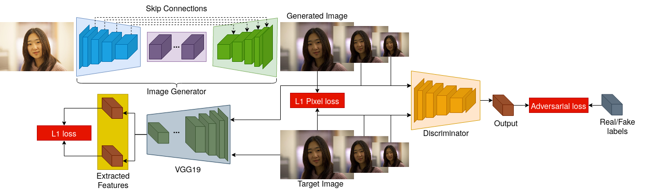
Figure 1: Proposed exposure correction method. Our generator contains encoder to embed the input image, residual block to edit the feature representation, and image decoder that is responsible to synthesize the output image. Perceptual loss, L1 pixel loss, and multi-scale discriminator lead to improve the performance.

3 Exposure correction

In this study, our main goal is to correct the exposure of the input image. Our model receives an image to manipulate the exposure setting in the feature space to synthesize the corrected version. There are three crucial points that we must address. 1) We must preserve the content of the image and only modify the exposure setting. 2) The input image can be underexposed or overexposed, therefore, we must learn the exposure correction for both cases without prior knowledge. 3) As we do not provide prior knowledge to the network about the exposure setting of the input image, we must also consider the scenario in which the input image has the correct exposure setting. In this case, our model must have the capacity to discover that the image has no exposure issue and must sustain the same exposure setting. Consequently, we address the exposure correction task for underexposed, overexposed, and well exposed cases by an end-to-end generative adversarial network based approach [14].

Generator. Given an input image $x\in\mathbb{R}^{W\times H\times 3}$, the objective of the image generator $G$ is to synthesize an output image $y^{\prime}\in\mathbb{R}^{W\times H\times 3}$ that must have the correct exposure setting. Besides, $G$ must learn not to alter the image with a correct exposure setting. The proposed $G$ involves three different submodules; image encoder $E_{img}$, residual block $R$ [18], and image decoder $D_{img}$. First, we extract image features $\phi_{x}\in\mathbb{R}^{512\times 16\times 16}$ using the image encoder $E_{img}$ and then forward it through the consecutive residual blocks in order to edit the feature representation. In the end, the altered features pass through the image decoder to generate the final output $y^{\prime}$. Moreover, we employ several residual connections between reciprocal convolutional layers of the image encoder $E_{img}$ and decoder $D_{img}$ to preserve the intermediate feature representation of $E_{img}$ in the decoder $D_{img}$. The proposed image generator $G$ is illustrated in Figure 1. Our image generator has five consecutive convolutional layers with ReLU activation function [43, 25] and Instance Normalization layer [49]. Similarly, the proposed image decoder contains five consecutive transposed convolutional layer with ReLU and Instance Norm to synthesize images.

Discriminator. We employ a discriminator network $D$ to distinguish between real samples and fake samples. The proposed $D$ is presented in Figure 1. It contains several consecutive convolutional layers to downsample the image to produce an output representation. We employ spectral normalization [42] after the convolutional layers to normalize the spectral norm of the weight matrices. This helps us to make the training more stable as well as to bound the Lipschitz norm $\sigma(W)=1$. Moreover, we propose to use multiple discriminators [10]. For this, we utilize three identical discriminators at three different scales [53]. According to our preliminary experimental analysis, this multi-scale discriminator approach improves to capture both the global structure and details of the images simultaneously and leads to synthesizing high-resolution images in better quality. The discriminator network involves five consecutive convolutional layers with spectral normalization [42] and Leaky ReLU activation function [40].

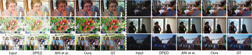
Figure 2: The results on exposure correction dataset [2]. We take images from [2] and compare with our model.

Method	Expert A		Expert B		Expert C		Expert D		Expert E		Avg		PI
	PSNR	SSIM	PSNR	SSIM	PSNR	SSIM	PSNR	SSIM	PSNR	SSIM	PSNR	SSIM
WVM [12]	12.355	0.624	13.147	0.656	12.748	0.645	14.059	0.669	15.207	0.690	13.503	0.657	2.342
LIME* [16, 17]	09.627	0.549	10.096	0.569	9.875	0.570	10.936	0.597	11.903	0.626	10.487	0.582	2.412
HDR CNN w/ PS [9]	14.804	0.651	15.622	0.689	15.348	0.670	16.583	0.685	18.022	0.703	16.076	0.680	2.248
DPED (iPhone) [21]	12.680	0.562	13.422	0.586	13.135	0.581	14.477	0.596	15.702	0.630	13.883	0.591	2.909
DPED (BlackBerry) [21]	15.170	0.621	16.193	0.691	15.781	0.642	17.042	0.677	18.035	0.678	16.444	0.662	2.518
DPE (HDR) [8]	14.399	0.572	15.219	0.573	15.091	0.593	15.692	0.581	16.640	0.626	15.408	0.589	2.417
DPE (S-FiveK) [8]	14.786	0.638	15.519	0.649	15.625	0.668	16.586	0.664	17.661	0.684	16.035	0.661	2.621
RetinexNet* [55]	10.149	0.570	10.880	0.586	10.471	0.595	11.498	0.613	12.295	0.635	11.059	0.600	2.933
Deep UPE* [51]	10.047	0.532	10.462	0.568	10.307	0.557	11.583	0.591	12.639	0.619	11.008	0.573	2.428
Zero-DCE [15]	10.116	0.503	10.767	0.502	10.395	0.514	11.471	0.522	12.354	0.557	11.021	0.519	2.774
Afifi et al. w/o $L_{adv}$ [2]	18.976	0.743	19.767	0.731	19.980	0.768	18.966	0.716	19.056	0.727	19.349	0.737	2.189
Afifi et al. w/ $L_{adv}$  [2]	18.874	0.738	19.569	0.718	19.788	0.760	18.823	0.705	18.936	0.719	19.198	0.728	2.183
Ours	20.475	0.862	21.833	0.891	22.438	0.901	20.127	0.874	20.062	0.881	20.987	0.881	2.158
WVM [12]	17.686	0.728	19.787	0.764	18.670	0.728	18.568	0.729	18.362	0.724	18.615	0.735	2.525
LIME* [16, 17]	13.444	0.653	14.426	0.672	13.980	0.663	15.190	0.673	16.177	0.694	14.643	0.671	2.462
HDR CNN w/ PS [9]	17.324	0.692	18.992	0.714	18.047	0.696	18.377	0.689	19.593	0.701	18.467	0.698	2.294
DPED (iPhone) [21]	18.814	0.680	21.129	0.712	20.064	0.683	19.711	0.675	19.574	0.676	19.858	0.685	2.894
DPED (BlackBerry) [21]	19.519	0.673	22.333	0.745	20.342	0.669	19.611	0.683	18.489	0.653	20.059	0.685	2.633
DPE (HDR) [8]	17.625	0.675	18.542	0.705	18.127	0.677	16.831	0.665	15.891	0.643	17.403	0.673	2.340
DPE (S-FiveK) [8]	20.153	0.738	20.973	0.697	20.915	0.738	19.050	0.688	17.510	0.648	19.720	0.702	2.564
RetinexNet* [55]	11.676	0.607	12.711	0.611	12.132	0.621	12.720	0.618	13.233	0.637	12.494	0.619	3.362
Deep UPE* [51]	17.832	0.728	19.059	0.754	18.763	0.745	19.641	0.737	20.237	0.740	19.106	0.741	2.371
Zero-DCE [15]	13.935	0.585	15.239	0.593	14.552	0.589	15.202	0.587	15.893	0.614	14.964	0.593	3.001
Afifi et al. w/o $L_{adv}$  [2]	19.432	0.750	20.590	0.739	20.542	0.770	18.989	0.723	18.874	0.727	19.685	0.742	2.344
Afifi et al. w/ $L_{adv}$  [2]	19.475	0.751	20.546	0.730	20.518	0.768	18.935	0.715	18.756	0.719	19.646	0.737	2.342
Ours	20.397	0.858	21.683	0.883	22.175	0.893	19.771	0.865	19.508	0.867	20.706	0.873	2.375
WVM [12]	14.488	0.665	15.803	0.699	15.117	0.678	15.863	0.693	16.469	0.704	15.548	0.688	2.415
LIME* [16, 17]	11.154	0.591	11.828	0.610	11.517	0.607	12.638	0.628	13.613	0.653	12.150	0.618	2.432
HDR CNN w/ PS [9]	15.812	0.667	16.970	0.699	16.428	0.681	17.301	0.687	18.650	0.702	17.032	0.687	2.267
DPED (iPhone) [21]	15.134	0.609	16.505	0.636	15.907	0.622	16.571	0.627	17.251	0.649	16.274	0.629	2.903
DPED (BlackBerry) [21]	16.910	0.642	18.649	0.713	17.606	0.653	18.070	0.679	18.217	0.668	17.890	0.671	2.564
DPE (HDR) [8]	15.690	0.614	16.548	0.626	16.305	0.626	16.147	0.615	16.341	0.633	16.206	0.623	2.417
DPE (S-FiveK) [8]	16.933	0.678	17.701	0.668	17.741	0.696	17.572	0.674	17.601	0.670	17.510	0.677	2.621
RetinexNet* [55]	10.759	0.585	11.613	0.596	11.135	0.605	11.987	0.615	12.671	0.636	11.633	0.607	3.105
Deep UPE* [51]	13.161	0.610	13.901	0.642	13.689	0.632	14.806	0.649	15.678	0.667	14.247	0.640	2.405
Zero-DCE [15]	11.643	0.536	12.555	0.539	12.058	0.544	12.964	0.548	13.769	0.580	12.597	0.549	2.865
Afifi et al. w/o $L_{adv}$  [2]	19.158	0.746	20.096	0.734	20.205	0.769	18.975	0.719	18.983	0.727	19.483	0.739	2.251
Afifi et al. w/ $L_{adv}$  [2]	19.114	0.743	19.960	0.723	20.080	0.763	18.868	0.709	18.864	0.719	19.377	0.731	2.247
Ours	20.443	0.860	21.773	0.887	22.332	0.897	19.984	0.870	19.840	0.875	20.874	0.877	2.244

Table 1: Exposure correction results on exposure dataset[2]. We highlight the best results with green and the second-best results with yellow. $*$ shows the methods that were trained for only the underexposure case. We divide the table into three subgroups: 1) well- and overexposure (3543 images), 2) underexposure (2362 images), 3) altogether case (5905 images).

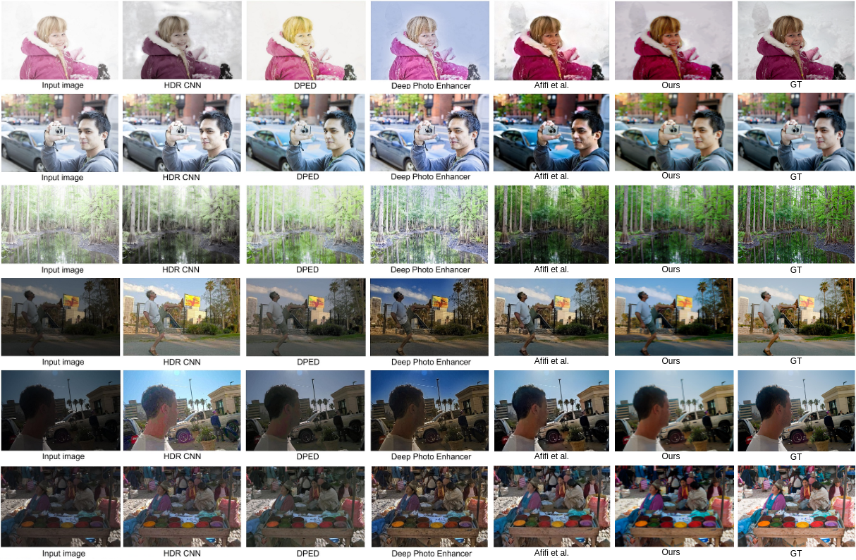
Figure 3: We take outputs of other models from [2] and compare with our results and ground truth images from expert A.

3.1 Learning procedure

The outputs of our multi-scale discriminator are $\mathbb{R}^{N\times N\times 1},N=16,32,64$. We use these feature representations of real and fake samples in the adversarial loss. For this, we create real and fake matrices with one and zero values as the discriminator output. and we calculate MSE between them. Besides, we utilize improved adversarial loss [53] to stabilize the training by extracting features from different levels of the discriminator and calculate L1 distance to perform feature matching at different scales. Additionally, we benefit from the perceptual loss [23] by extracting features from the real and fake samples using the VGG-19 network [47] to compare the L1 distance in the feature space. The corresponding loss function is shown in Equation 1.

$$L_{per}=\sum_{i=1}^{5}(c_{i}||(L^{i}(y^{\prime})-L^{i}(y)||_{1}$$ (1)

We use five different layers to extract features and calculate the loss [23]. Furthermore, we employ L1 distance loss in the pixel space to directly compare the generated image and the ground truth image: $L_{pixel}=||y^{\prime}-y||_{1}$. The overall loss is presented in Equation 2.

$$L=L_{GAN}(G,D)+\lambda L_{pixel}(G)+\beta L_{per}(G)$$ (2)

Utilized coefficients $\lambda$ and $\beta$ adjust the effect of each loss over the final loss. We empirically find the best values on the validation set of  [2] as 0.5 and 1, respectively.

4 Experimental Result

4.1 Datasets

Exposure correction dataset. We train our model on a novel large-scale exposure correction dataset [2] which has underexposed, overexposed, well-exposed, and ground truth images. We follow the same setup in [2]. The training set contains 17675 images, while the validation set has 750 images. Lastly, the test set consists of 5905 images with five different versions: well-exposed, underexposed with -1 and -1.5 EVs, and overexposed with +1 and +1.5 EVs.

Portrait matting datasets. We also investigate the effect of under- and overexposed images over the portrait matting performance. For this, we choose four different real-world portrait matting datasets. Since we manipulate the exposure setting of the images, we need to have real-world images to investigate the exposure accurately. In order to perform this analysis, we utilize PPM-100 [24], P3M500 [31], RWP636 [60], and AIM500 [33] datasets. These datasets contain 100, 500, 636, and 500 images, respectively. Please note that AIM500 [33] is proposed for general image matting, therefore, we only select portrait images from this dataset. In the end, we have 100 images for this dataset. We use Adobe Photoshop Lightroom to digitally manipulate the exposure setting of these datasets to obtain under- and overexposed images by utilizing -1.5, -1, +1, and +1.5 values. For further investigation, we also utilize -2, -2.5, +2, and +2.5 EVs to change the exposure setting more. With this additional manipulation, we both examine the effect of severe exposure errors and the performance of the exposure correction model beyond the used cases in the training.

4.2 Evaluation

In order to assess the exposure correction performance, we follow the literature and use three evaluation metrics: peak signal-to-noise ratio (PSNR), structural similarity index measure (SSIM) [54], and perceptual index (PI) [4] which is ground truth-free evaluation method and is the combination of Ma [37] and NIQE [41] metrics.

In order to evaluate the effect of the exposure setting over the portrait matting, we decide to use three state-of-the-art matting methods that do not need to have an additional input to produce an alpha matte. We utilize MODNet [24], MGMatting (MGM) [60], and GFM [32]. We run these models with well-, under-, and overexposed images to generate alpha matte. Then, we repeat the same experiments with the images in which their exposure setting is corrected by our exposure correction model. To evaluate the outputs, we use two commonly used metrics in the matting literature: mean squared error (MSE) and mean absolute error (MAE).

4.3 Exposure Correction Results

In Table 1, we present the results on exposure correction dataset [2]. We follow the same analysis in [2] and split the table into three separate groups. In the first group, we show the results for well- and overexposed images that are obtained with $0,+1,+1.5$ EVs. This test setup contains 3543 images. In the second one, we demonstrate the results for underexposure cases, with EVs of $-1$ and $-1.5$. This test setup involves 2362 images. In the last group, we present the results for all cases and this includes all 5905 images.

The corresponding dataset has five different ground truth images for each input, namely expert A, expert B, expert C, expert D, expert E. Therefore, we provide the results for all of these five experts separately. In the end, we also calculate the average results over these expert sets. Please note that we acquire all these results, except Ours, from the corresponding paper [2]. Experimental results show that our proposed method outperforms all other methods for all scenarios, experts, and metrics. Only two exceptions are DPED (BlackBerry) method that achieves slightly better PSNR result for underexposure scenario for Expert B ground truth set and Deep UPE method which obtains slightly higher PSNR score for Expert E case. Please note that Deep UPE was proposed for only underexposure problem. Because of that it is more likely for it to achieve better performance for the underexposure scenario in theory. However, our proposed method surpasses DPED (BlackBerry) and Deep UPE models in terms of the SSIM metric for Expert B and Expert E. Besides, for the rest of the experts, our method surpasses all other methods in both metrics. In summary, our method has the best average scores as can be seen from the last row of Table 1, since the proposed system has more complex and effective architecture with residual connections for conditional image generation. Moreover, utilized loss functions and multi-scale discriminator improve the quality of the generated image and make the learning procedure more stable. With the help of all these components, the proposed system is able to adjust the exposure setting without modifying the content. Please note that, Deep UPE, RetinexNet, and LIME models are specifically developed for the underexposure case only. However, although our proposed method is not specifically designed for underexposure correction, it still outperforms these models on average for the underexposure case. In Table 2, we present the results of recent works on exposure correction dataset [2]. According to the table, our proposed model achieves state-of-the-art results by surpassing all other methods on three different metrics.

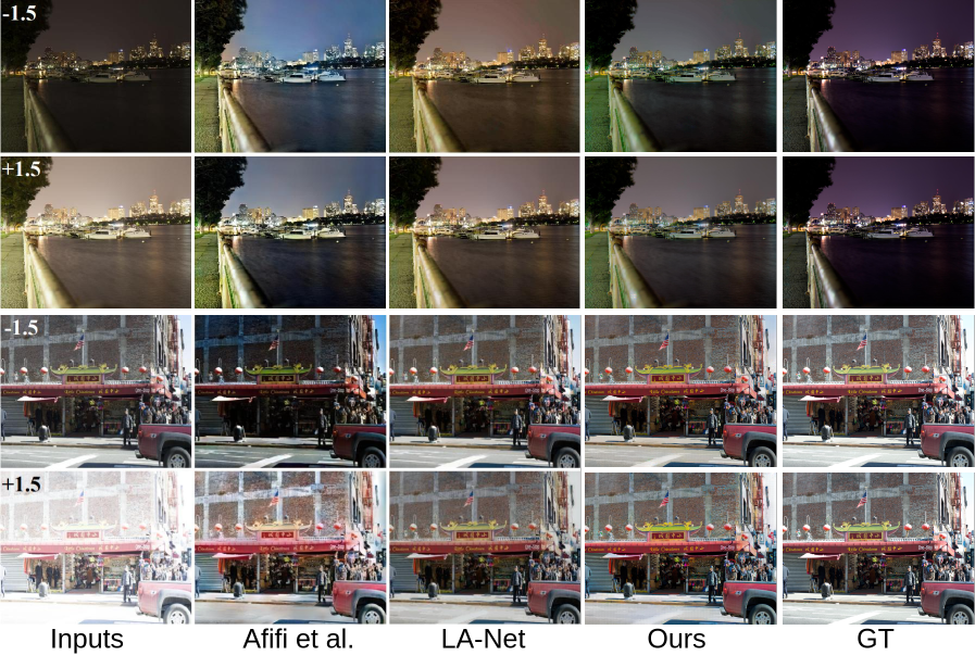
Figure 4: Visual comparisons of sample images with under- and overexposure conditions. We compare our results with Afifi et al. [2], LA-Net [58], and ground truth images.

Method	PSNR $\uparrow$	SSIM $\uparrow$	PI $\downarrow$
Afifi et al. w/o $L_{adv}$  [2]	19.48	0.73	2.251
Afifi et al. w/ $L_{adv}$  [2]	19.37	0.73	2.247
LA-Net [58]	20.70	0.81	2.353
FCN SEC [34]	19.71	0.80	-
FCN MEF [34]	20.81	0.84	-
Ours	20.87	0.87	2.244

Table 2: Summary of exposure correction results on [2]. We achieve the state-of-the-art result on all three metrics.

In Figure 2, 3, 4, we present different test images, our results, ground truth images, and the results of other models. We obtain the corresponding outputs for other models from their papers in order to compare with our results. As one can see from Figure 2 and Figure 3, our results are closer to the ground truth images than the other methods. Besides, our results have better quality in the details and provide a more similar color distribution with the ground truth images. In Figure 4, we provide four different cases and our model can accurately correct the exposure problem, although all three models have a problem in the color distribution of the first image due to the challenging lighting condition.

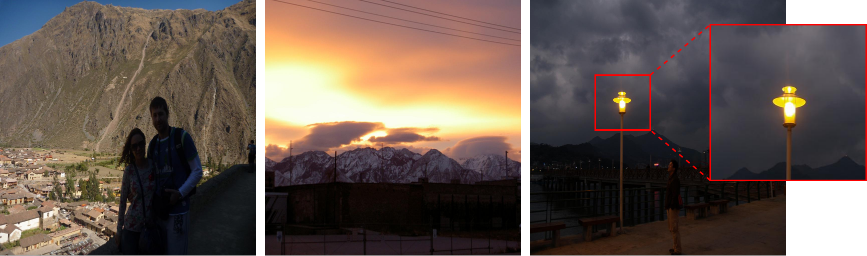
Inputs

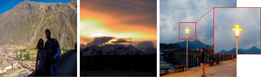
Outputs

Figure 5: Failure cases. The model may fail when the image includes locally under- and overexposed parts. Output may also have artifacts around light sources, despite well corrected exposure.

Method	LIME [17]	NPE [52]	VV [50]	DICM [27]	Avg.
NPE [52]	3.91	3.95	2.52	3.76	3.54
LIME [17]	4.16	4.26	2.49	3.85	3.69
WVM [12]	3.79	3.99	2.85	3.90	3.63
RNet [55]	4.42	4.49	2.60	4.20	3.93
KinD [66]	3.72	3.88	-	-	3.80
EGAN [22]	3.72	4.11	2.58	-	3.50
DBCP [29]	3.78	3.18	-	3.57	3.48
Afifi et al. [2]	3.76	3.18	2.28	2.50	2.93
Ours	3.12	2.90	2.98	3.02	3.01

Table 3: Results on four low-light image datasets. We follow the literature and provide NIQE metric on these datasets. Lower results indicate better performance.

Data	Method	-2.5		-2		-1.5		-1		0		1		1.5		2		2.5		Avg
		MSE	MAE	MSE	MAE	MSE	MAE	MSE	MAE	MSE	MAE	MSE	MAE	MSE	MAE	MSE	MAE	MSE	MAE	MSE	MAE
PPM-100 E	MODNet	10.1	16.7	8.6	15.0	7.3	13.8	6.1	12.1	5.8	11.5	5.6	11.5	6.6	12.6	6.7	12.7	10	16.4	7.42	13.59
PPM-100 C	MODNet	7.8	13.4	6.9	12.5	6.6	12.2	6.6	12.2	6.2	11.7	6.0	11.1	6.0	11.2	5.7	11.7	6.0	12.5	6.42	12.05
P3M500 E	MODNet	9.9	17.3	8.7	16.0	8.1	15.0	7.8	14.7	7.5	14.3	10.2	16.9	11.8	18.5	14.5	21.6	19.7	27.5	10.91	17.97
P3M500 C	MODNet	7.8	14	7.0	13.1	6.9	13.1	6.6	12.7	6.1	11.9	6.2	12.2	6.5	12.5	7.4	13.4	10.0	16.1	7.26	13.22
RWP636 E	MODNet	27.2	41.8	24.8	39.3	22.5	36.8	22.1	35.4	24.3	38.0	27.6	41.7	33.9	48.4	40.7	55.5	50.7	66.0	30.42	44.76
RWP636 C	MODNet	22.4	35.4	21.9	34.9	21.4	34.4	20.5	33.4	19.9	32.1	20.3	33.1	20.4	33.4	21.5	34.5	24.5	37.5	21.42	34.30
AIM500 E	MODNet	11.5	18.2	10.8	17.4	10.1	16.5	10.0	16.3	10.0	16.3	12.1	18.1	13.1	19.3	15.3	22.0	19.4	26.7	12.47	18.97
AIM500 C	MODNet	10.9	17.0	10.6	16.8	10.6	16.7	9.9	15.9	9.8	15.8	10.4	16.2	10.7	16.6	10.4	16.3	11.7	17.7	10.55	16.55
PPM-100 E	MGM	1.6	6.3	1.3	5.9	1.3	5.6	1.2	5.4	1.2	5.3	1.4	5.7	1.6	6.1	1.8	6.5	2.0	7.0	1.49	5.98
PPM-100 C	MGM	1.3	5.8	1.3	5.7	1.3	5.6	1.2	5.4	1.3	5.7	1.3	5.7	1.3	5.7	1.3	5.8	1.4	6.0	1.30	5.71
P3M500 E	MGM	4.3	10.5	4.3	10.3	3.8	9.4	3.6	8.9	3.5	8.3	3.6	8.6	4.1	9.6	4.9	11.1	6.5	14.2	4.29	10.10
P3M500 C	MGM	3.7	9.1	3.7	9.1	3.6	9.0	3.6	8.9	3.5	8.7	3.6	8.8	3.6	9.0	3.9	9.6	5.4	12.8	3.84	9.44
RWP636 E	MGM	9.2	21.0	9.1	20.7	8.9	20.5	8.8	20.2	8.7	19.7	9.2	20.2	9.6	21.0	10.2	22.1	11.3	24.4	9.44	21.08
RWP636 C	MGM	9.0	20.2	9.0	20.2	9.0	20.2	8.8	20.1	8.7	19.7	8.9	20.1	9.0	20.2	9.1	20.5	9.6	21.3	9.01	20.27
AIM500 E	MGM	4.4	10.9	4.2	10.3	4.1	9.8	4.3	9.7	5.8	10.6	5.0	10.0	5.6	11.2	6.6	13.2	7.8	16.1	5.31	11.31
AIM500 C	MGM	3.9	9.3	3.6	9.0	3.7	9.0	3.8	9.0	3.7	8.6	4.2	9.1	3.9	9.1	3.4	8.5	4.3	10.0	3.83	9.06
PPM-100 E	GFM	14.3	14.9	14.0	14.5	14.0	14.5	13.9	14.3	13.6	14.1	13.3	13.8	13.5	14.0	14.2	14.7	15.2	15.7	14.00	14.50
PPM-100 C	GFM	13.4	13.9	13.2	13.7	13.5	13.9	13.6	14.0	13.7	14.1	13.7	14.2	13.4	13.9	12.7	13.2	13.0	13.5	13.35	13.82
P3M500 E	GFM	8.4	9.0	8.4	9.0	8.5	9.1	8.6	9.1	9.4	9.9	11.0	11.5	12.1	12.6	13.2	13.7	14.7	15.2	10.48	11.01
P3M500 C	GFM	13.1	13.6	13.3	13.8	13.4	14.0	13.6	14.1	14.0	14.5	14.5	15.0	14.7	15.2	14.9	15.4	15.2	15.7	14.07	14.58
RWP636 E	GFM	13.7	14.9	14.1	15.3	14.4	16.0	13.2	14.7	12.9	14.1	17.7	18.7	19.2	20.2	21.0	22.2	23.8	24.8	16.67	17.88
RWP636 C	GFM	13.7	14.9	13.9	15.1	14.1	15.8	13.0	14.5	12.9	14.1	15.6	16.7	15.7	16.9	15.9	17.0	16.1	17.3	14.63	15.81
AIM500 E	GFM	6.8	7.4	6.6	7.1	6.5	7.0	6.5	7.0	6.4	6.9	8.4	8.9	9.3	9.8	10.2	10.7	11.8	12.4	8.05	8.58
AIM500 C	GFM	10.3	10.8	10.4	10.9	11.0	11.5	10.9	11.4	11.1	11.5	10.9	11.4	11.2	11.7	11.0	11.5	11.5	12.0	10.92	11.41

Table 4: Analysis of exposure correction in portrait matting task. White rows with E symbol indicates the manipulated images with the corresponding EV and C symbol in the gray rows states the corrected version of this corresponding image.

Generalization. We further perform additional tests on the four popular low-light image enhancement datasets in the literature, namely LIME [17], NPE [52], VV [50], and DICM [27], and compare our method with the existing methods in the literature. We demonstrate this analysis in Table 3. Some of these datasets also contain challenging images that have under- and overexposed regions at the same time. The proposed method is found to be superior compared to the existing methods on LIME and NPE datasets, and achieve comparable results on VV and DICM datasets. This outcome indicates that our model is well-generalized and is able to work on unseen datasets.

Limitations. In Figure 5, some failure examples from the low-light image enhancement datasets are shown. In the first column, the model can correct the exposure of the background scene, however, bottom right part still suffers from the underexposure problem. This should be investigated in detail in the future work, since containing this kind of local exposure problems may sometimes be challenging. Although our proposed model can accurately adjust exposure values of the images, some cases could be difficult to handle and cause artifacts around the light sources due to the intense light changes. This can be seen from the second and third examples in Figure 5.

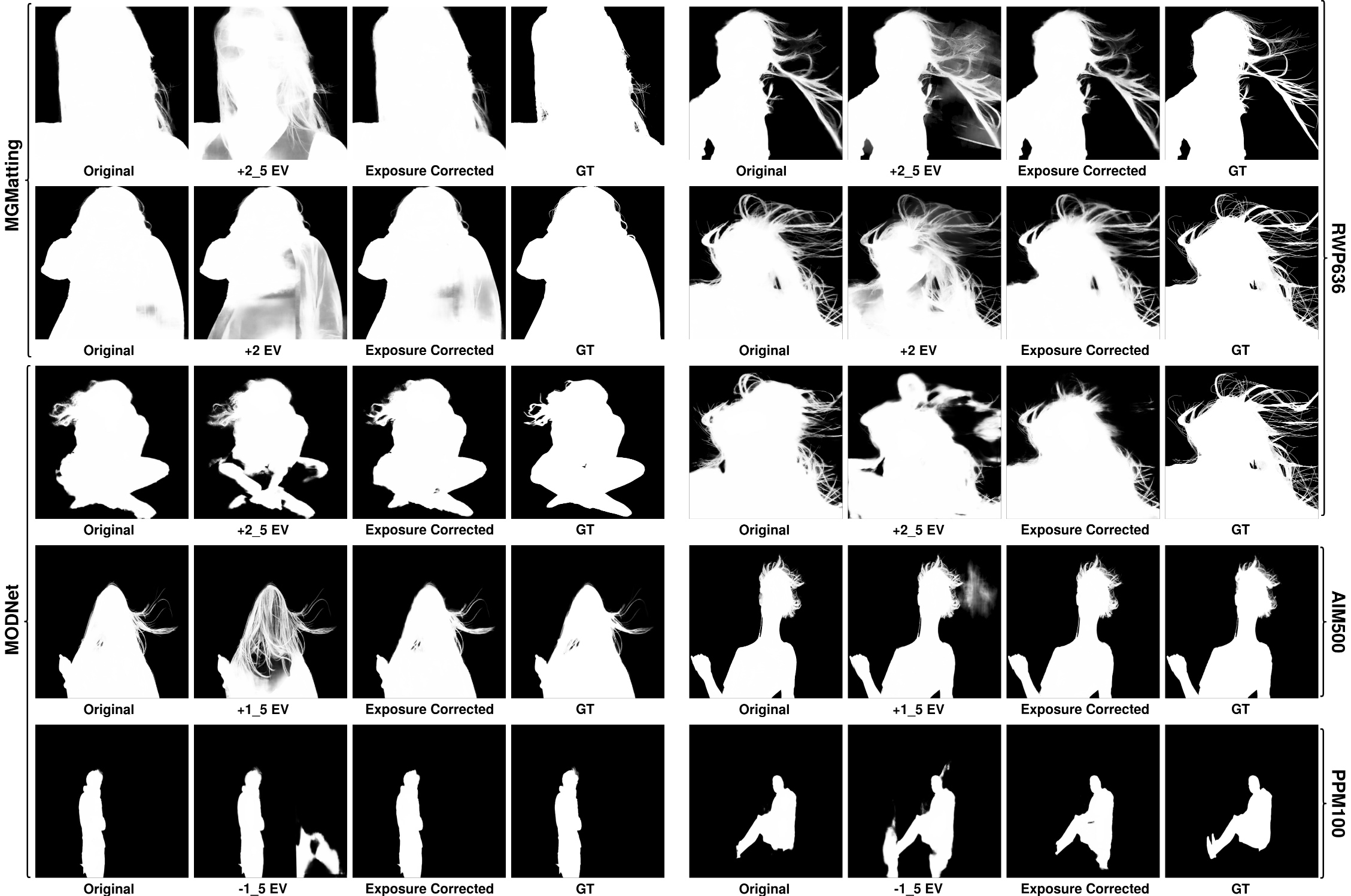
Figure 6: Illustration of the portrait matting outputs. We show sample images from RWP636, AIM500, and PPM100 datasets with MGMatting and MODNet models. The outputs of the remaining models and datasets are the same with this case.

4.4 Effect of exposure on portrait matting

Portrait matting models are generally too sensitive to the illumination condition of an image. The models have a difficulty to distinguish background scene and foreground subject precisely when the scene is too dark or too bright. Therefore, we perform further experiments in order to investigate the effect of exposure setting, namely well-, under-, and overexposed images, on the portrait matting task. The experimental results are presented in Table 4. In the table, letter E in the data column indicates the case in which the exposure setting of the images is manipulated with the corresponding EVs, that are presented on the top of the table. Similarly, letter C expresses the corrected images by our exposure correction model. In the experiments, we first manipulate the exposure settings of the images to have under- and overexposed images. Then, we perform portrait matting with the well-, under, and overexposed images. Afterward, we employ our exposure correction model, which is trained on the exposure correction dataset [2]. Finally, we test the portrait matting models on these corrected images. We also run experiments with the images that no exposure value is applied and present the results under 0 column.

As we can see from the table, the performance of the portrait matting models decreases when the input is under- or overexposed. While the best portrait matting performance is obtained with the original images, either by using them directly or by using the corrected version, the models show the worst performance with -2.5 and +2.5 EVs. The performances of the portrait matting models are improved significantly using the corrected versions of the under- and overexposed images. In some cases, the portrait matting models produce a better performance on the corrected version of the original images. This indicates that our exposure correction model enhances even the original images resulting in better portrait matting performance. Although portrait matting models’ performances decrease when the under- and overexposure level increases, the models show almost the same performance after the correction. These results show that our model is remarkably robust against different types and levels of exposure errors. The portrait matting models are found to perform better on underexposed images than overexposed images. In other words, overexposed images are more challenging for the portrait matting methods. After the correction, the models show almost the same performance on under- and overexposed images.

The exposure correction dataset [2] has samples with EVs of -1.5, -1, 0, +1, +1.5. However, in our test set for portrait matting, we also generate images with -2.5, -2, +2, +2.5 EVs. In this way, we are able to explicitly explore the performance of our exposure correction model for unseen cases, as our model was not trained on them. The results show that our model is able to enhance the images outside the training range. This demonstrates the generalization capacity of our exposure correction model.

In Figure 6, we show sample results for portrait matting task. In the figure, original column indicates the alpha matte prediction from the original image. The next column demonstrates the predicted results from the input images with different exposure settings. The applied EVs are presented under each image. The third column contains the alpha matte prediction from the corrected version of the under- and overexposed images. Finally, the last column demonstrates the ground truth alpha matte. All these results clearly show the severe degradation in the alpha matte prediction when the input is under- or overexposed image, independent of the employed alpha matte models and datasets. Similarly, when we correct the exposure of the image, the alpha matte prediction performance significantly increases and achieves the similar performance with the original input. This outcome indicates the necessity and usefulness of an exposure correction model as a preprocessing step before the portrait matting.

5 Conclusion

The exposure setting affects the quality and visibility of an image. In this paper, we propose an end-to-end model to address both under- and overexposure problems. We test our model on a large-scale exposure correction dataset and achieve the SOTA results. Besides, we analyze the effect of exposure error on the portrait matting task. For this, we choose three SOTA portrait matting methods and four real-world datasets to perform the experiments. Experimental results show that exposure setting affects the portrait matting performance significantly. The proposed exposure correction approach is found to be successful to eliminate the effects of under- and overexposure and able to recover the portrait matting performance. In the future work, we will focus on task-specific adaptations to improve the performance as well as increase the stability, especially when the images have under- and overexposed images together. Besides, we will compare different exposure correction models’ performance on portrait matting task to compare with our model.

Acknowledgement. The project on which this report is based was funded by the Federal Ministry of Education and Research (BMBF) of Germany under the number 01IS18040A.

References

- [1] Mahmoud Afifi and Michael S Brown. Deep white-balance editing. In Proceedings of the IEEE/CVF Conference on computer vision and pattern recognition, pages 1397–1406, 2020.
- [2] Mahmoud Afifi, Konstantinos G Derpanis, Bjorn Ommer, and Michael S Brown. Learning multi-scale photo exposure correction. In Proceedings of the IEEE/CVF Conference on Computer Vision and Pattern Recognition, pages 9157–9167, 2021.
- [3] Marwan Ali Albahar. Contrast and synthetic multiexposure fusion for image enhancement. Computational Intelligence and Neuroscience, 2021, 2021.
- [4] Yochai Blau, Roey Mechrez, Radu Timofte, Tomer Michaeli, and Lihi Zelnik-Manor. The 2018 pirm challenge on perceptual image super-resolution. In Proceedings of the European Conference on Computer Vision (ECCV) Workshops, pages 0–0, 2018.
- [5] Bolun Cai, Xianming Xu, Kailing Guo, Kui Jia, Bin Hu, and Dacheng Tao. A joint intrinsic-extrinsic prior model for retinex. In Proceedings of the IEEE international conference on computer vision, pages 4000–4009, 2017.
- [6] Jianrui Cai, Shuhang Gu, and Lei Zhang. Learning a deep single image contrast enhancer from multi-exposure images. IEEE Transactions on Image Processing, 27(4):2049–2062, 2018.
- [7] Turgay Celik and Tardi Tjahjadi. Contextual and variational contrast enhancement. IEEE Transactions on Image Processing, 20(12):3431–3441, 2011.
- [8] Yu-Sheng Chen, Yu-Ching Wang, Man-Hsin Kao, and Yung-Yu Chuang. Deep photo enhancer: Unpaired learning for image enhancement from photographs with gans. In Proceedings of the IEEE Conference on Computer Vision and Pattern Recognition, pages 6306–6314, 2018.
- [9] Lisa DaNae Dayley and Brad Dayley. Photoshop CS5 Bible. John Wiley & Sons, 2010.
- [10] Ishan Durugkar, Ian Gemp, and Sridhar Mahadevan. Generative multi-adversarial networks. arXiv preprint arXiv:1611.01673, 2016.
- [11] Majed El Helou, Ruofan Zhou, Sabine Susstrunk, and Radu Timofte. Ntire 2021 depth guided image relighting challenge. In Proceedings of the IEEE/CVF Conference on Computer Vision and Pattern Recognition, pages 566–577, 2021.
- [12] Xueyang Fu, Delu Zeng, Yue Huang, Xiao-Ping Zhang, and Xinghao Ding. A weighted variational model for simultaneous reflectance and illumination estimation. In Proceedings of the IEEE conference on computer vision and pattern recognition, pages 2782–2790, 2016.
- [13] Michaël Gharbi, Jiawen Chen, Jonathan T Barron, Samuel W Hasinoff, and Frédo Durand. Deep bilateral learning for real-time image enhancement. ACM Transactions on Graphics (TOG), 36(4):1–12, 2017.
- [14] Ian Goodfellow, Jean Pouget-Abadie, Mehdi Mirza, Bing Xu, David Warde-Farley, Sherjil Ozair, Aaron Courville, and Yoshua Bengio. Generative adversarial nets. Advances in neural information processing systems, 27, 2014.
- [15] Chunle Guo, Chongyi Li, Jichang Guo, Chen Change Loy, Junhui Hou, Sam Kwong, and Runmin Cong. Zero-reference deep curve estimation for low-light image enhancement. In Proceedings of the IEEE/CVF Conference on Computer Vision and Pattern Recognition, pages 1780–1789, 2020.
- [16] Xiaojie Guo. Lime: A method for low-light image enhancement. In Proceedings of the 24th ACM international conference on Multimedia, pages 87–91, 2016.
- [17] Xiaojie Guo, Yu Li, and Haibin Ling. Lime: Low-light image enhancement via illumination map estimation. IEEE Transactions on image processing, 26(2):982–993, 2016.
- [18] Kaiming He, Xiangyu Zhang, Shaoqing Ren, and Jian Sun. Deep residual learning for image recognition. In Proceedings of the IEEE conference on computer vision and pattern recognition, pages 770–778, 2016.
- [19] Haofeng Huang, Wenhan Yang, Yueyu Hu, Jiaying Liu, and Ling-Yu Duan. Towards low light enhancement with raw images. IEEE Transactions on Image Processing, 2022.
- [20] Haidi Ibrahim and Nicholas Sia Pik Kong. Brightness preserving dynamic histogram equalization for image contrast enhancement. IEEE Transactions on Consumer Electronics, 53(4):1752–1758, 2007.
- [21] Andrey Ignatov, Nikolay Kobyshev, Radu Timofte, Kenneth Vanhoey, and Luc Van Gool. Dslr-quality photos on mobile devices with deep convolutional networks. In Proceedings of the IEEE International Conference on Computer Vision, pages 3277–3285, 2017.
- [22] Yifan Jiang, Xinyu Gong, Ding Liu, Yu Cheng, Chen Fang, Xiaohui Shen, Jianchao Yang, Pan Zhou, and Zhangyang Wang. Enlightengan: Deep light enhancement without paired supervision. IEEE Transactions on Image Processing, 30:2340–2349, 2021.
- [23] Justin Johnson, Alexandre Alahi, and Li Fei-Fei. Perceptual losses for real-time style transfer and super-resolution. In European conference on computer vision, pages 694–711. Springer, 2016.
- [24] Zhanghan Ke, Kaican Li, Yurou Zhou, Qiuhua Wu, Xiangyu Mao, Qiong Yan, and Rynson WH Lau. Is a green screen really necessary for real-time portrait matting? arXiv preprint arXiv:2011.11961, 2020.
- [25] Alex Krizhevsky, Ilya Sutskever, and Geoffrey E Hinton. Imagenet classification with deep convolutional neural networks. Advances in neural information processing systems, 25, 2012.
- [26] Edwin H Land. The retinex theory of color vision. Scientific american, 237(6):108–129, 1977.
- [27] Chulwoo Lee, Chul Lee, and Chang-Su Kim. Contrast enhancement based on layered difference representation. In 2012 19th IEEE international conference on image processing, pages 965–968. IEEE, 2012.
- [28] Chulwoo Lee, Chul Lee, and Chang-Su Kim. Contrast enhancement based on layered difference representation of 2d histograms. IEEE transactions on image processing, 22(12):5372–5384, 2013.
- [29] Hunsang Lee, Kwanghoon Sohn, and Dongbo Min. Unsupervised low-light image enhancement using bright channel prior. IEEE Signal Processing Letters, 27:251–255, 2020.
- [30] Chongyi Li, Chunle Guo, Ling-Hao Han, Jun Jiang, Ming-Ming Cheng, Jinwei Gu, and Chen Change Loy. Low-light image and video enhancement using deep learning: a survey. IEEE Transactions on Pattern Analysis & Machine Intelligence, (01):1–1, 2021.
- [31] Jizhizi Li, Sihan Ma, Jing Zhang, and Dacheng Tao. Privacy-preserving portrait matting. In Proceedings of the 29th ACM International Conference on Multimedia, pages 3501–3509, 2021.
- [32] Jizhizi Li, Jing Zhang, Stephen J Maybank, and Dacheng Tao. Bridging composite and real: towards end-to-end deep image matting. International Journal of Computer Vision, pages 1–21, 2022.
- [33] Jizhizi Li, Jing Zhang, and Dacheng Tao. Deep automatic natural image matting. arXiv preprint arXiv:2107.07235, 2021.
- [34] Jin Liang, Anran Zhang, Jun Xu, Hui Li, and Xiantong Zhen. Fusion-correction network for single-exposure correction and multi-exposure fusion. arXiv preprint arXiv:2203.03624, 2022.
- [35] Yuen Peng Loh and Chee Seng Chan. Getting to know low-light images with the exclusively dark dataset. Computer Vision and Image Understanding, 178:30–42, 2019.
- [36] Kin Gwn Lore, Adedotun Akintayo, and Soumik Sarkar. Llnet: A deep autoencoder approach to natural low-light image enhancement. Pattern Recognition, 61:650–662, 2017.
- [37] Chao Ma, Chih-Yuan Yang, Xiaokang Yang, and Ming-Hsuan Yang. Learning a no-reference quality metric for single-image super-resolution. Computer Vision and Image Understanding, 158:1–16, 2017.
- [38] Kede Ma, Zhengfang Duanmu, Hanwei Zhu, Yuming Fang, and Zhou Wang. Deep guided learning for fast multi-exposure image fusion. IEEE Transactions on Image Processing, 29:2808–2819, 2019.
- [39] Long Ma, Dian Jin, Risheng Liu, Xin Fan, and Zhongxuan Luo. Joint over and under exposures correction by aggregated retinex propagation for image enhancement. IEEE Signal Processing Letters, 27:1210–1214, 2020.
- [40] Andrew L Maas, Awni Y Hannun, Andrew Y Ng, et al. Rectifier nonlinearities improve neural network acoustic models. In Proc. icml, volume 30, page 3. Citeseer, 2013.
- [41] Anish Mittal, Rajiv Soundararajan, and Alan C Bovik. Making a “completely blind” image quality analyzer. IEEE Signal processing letters, 20(3):209–212, 2012.
- [42] Takeru Miyato, Toshiki Kataoka, Masanori Koyama, and Yuichi Yoshida. Spectral normalization for generative adversarial networks. arXiv preprint arXiv:1802.05957, 2018.
- [43] Vinod Nair and Geoffrey E Hinton. Rectified linear units improve restricted boltzmann machines. In Icml, 2010.
- [44] Zhangkai Ni, Wenhan Yang, Shiqi Wang, Lin Ma, and Sam Kwong. Towards unsupervised deep image enhancement with generative adversarial network. IEEE Transactions on Image Processing, 29:9140–9151, 2020.
- [45] Hao Ouyang, Zifan Shi, Chenyang Lei, Ka Lung Law, and Qifeng Chen. Neural camera simulators. In Proceedings of the IEEE/CVF Conference on Computer Vision and Pattern Recognition, pages 7700–7709, 2021.
- [46] Linhao Qu, Shaolei Liu, Manning Wang, and Zhijian Song. Transmef: A transformer-based multi-exposure image fusion framework using self-supervised multi-task learning. arXiv preprint arXiv:2112.01030, 2021.
- [47] Karen Simonyan and Andrew Zisserman. Very deep convolutional networks for large-scale image recognition. arXiv preprint arXiv:1409.1556, 2014.
- [48] Gabriel Thomas, Daniel Flores-Tapia, and Stephen Pistorius. Histogram specification: a fast and flexible method to process digital images. IEEE Transactions on Instrumentation and Measurement, 60(5):1565–1578, 2011.
- [49] Dmitry Ulyanov, Andrea Vedaldi, and Victor Lempitsky. Instance normalization: The missing ingredient for fast stylization. arXiv preprint arXiv:1607.08022, 2016.
- [50] Vassilios Vonikakis. Busting image enhancement and tonemapping algorithms.
- [51] Ruixing Wang, Qing Zhang, Chi-Wing Fu, Xiaoyong Shen, Wei-Shi Zheng, and Jiaya Jia. Underexposed photo enhancement using deep illumination estimation. In Proceedings of the IEEE/CVF Conference on Computer Vision and Pattern Recognition, pages 6849–6857, 2019.
- [52] Shuhang Wang, Jin Zheng, Hai-Miao Hu, and Bo Li. Naturalness preserved enhancement algorithm for non-uniform illumination images. IEEE transactions on image processing, 22(9):3538–3548, 2013.
- [53] Ting-Chun Wang, Ming-Yu Liu, Jun-Yan Zhu, Andrew Tao, Jan Kautz, and Bryan Catanzaro. High-resolution image synthesis and semantic manipulation with conditional gans. In Proceedings of the IEEE conference on computer vision and pattern recognition, pages 8798–8807, 2018.
- [54] Zhou Wang, Alan C Bovik, Hamid R Sheikh, and Eero P Simoncelli. Image quality assessment: from error visibility to structural similarity. IEEE transactions on image processing, 13(4):600–612, 2004.
- [55] Chen Wei, Wenjing Wang, Wenhan Yang, and Jiaying Liu. Deep retinex decomposition for low-light enhancement. arXiv preprint arXiv:1808.04560, 2018.
- [56] Ke Xu, Xin Yang, Baocai Yin, and Rynson WH Lau. Learning to restore low-light images via decomposition-and-enhancement. In Proceedings of the IEEE/CVF Conference on Computer Vision and Pattern Recognition, pages 2281–2290, 2020.
- [57] Huan Yang, Baoyuan Wang, Noranart Vesdapunt, Minyi Guo, and Sing Bing Kang. Personalized exposure control using adaptive metering and reinforcement learning. IEEE transactions on visualization and computer graphics, 25(10):2953–2968, 2018.
- [58] Kai-Fu Yang, Cheng Cheng, Shi-Xuan Zhao, Xian-Shi Zhang, and Yong-Jie Li. Learning to adapt to light. arXiv preprint arXiv:2202.08098, 2022.
- [59] Wenhan Yang, Shiqi Wang, Yuming Fang, Yue Wang, and Jiaying Liu. From fidelity to perceptual quality: A semi-supervised approach for low-light image enhancement. In Proceedings of the IEEE/CVF conference on computer vision and pattern recognition, pages 3063–3072, 2020.
- [60] Qihang Yu, Jianming Zhang, He Zhang, Yilin Wang, Zhe Lin, Ning Xu, Yutong Bai, and Alan Yuille. Mask guided matting via progressive refinement network. In Proceedings of the IEEE/CVF Conference on Computer Vision and Pattern Recognition, pages 1154–1163, 2021.
- [61] Runsheng Yu, Wenyu Liu, Yasen Zhang, Zhi Qu, Deli Zhao, and Bo Zhang. Deepexposure: Learning to expose photos with asynchronously reinforced adversarial learning. Advances in Neural Information Processing Systems, 31, 2018.
- [62] Feng Zhang, Yuanjie Shao, Yishi Sun, Kai Zhu, Changxin Gao, and Nong Sang. Unsupervised low-light image enhancement via histogram equalization prior. arXiv preprint arXiv:2112.01766, 2021.
- [63] Qing Zhang, Yongwei Nie, and Wei-Shi Zheng. Dual illumination estimation for robust exposure correction. In Computer Graphics Forum, volume 38, pages 243–252. Wiley Online Library, 2019.
- [64] Qing Zhang, Ganzhao Yuan, Chunxia Xiao, Lei Zhu, and Wei-Shi Zheng. High-quality exposure correction of underexposed photos. In Proceedings of the 26th ACM international conference on Multimedia, pages 582–590, 2018.
- [65] Yonghua Zhang, Xiaojie Guo, Jiayi Ma, Wei Liu, and Jiawan Zhang. Beyond brightening low-light images. International Journal of Computer Vision, 129(4):1013–1037, 2021.
- [66] Yonghua Zhang, Jiawan Zhang, and Xiaojie Guo. Kindling the darkness: A practical low-light image enhancer. In Proceedings of the 27th ACM international conference on multimedia, pages 1632–1640, 2019.
- [67] Minfeng Zhu, Pingbo Pan, Wei Chen, and Yi Yang. Eemefn: Low-light image enhancement via edge-enhanced multi-exposure fusion network. In Proceedings of the AAAI Conference on Artificial Intelligence, volume 34, pages 13106–13113, 2020.
- [68] Karel Zuiderveld. Contrast limited adaptive histogram equalization. Graphics gems, pages 474–485, 1994.