Simulating active agents under confinement with Dissipative Particles (hydro)Dynamics

Abstract

In this work we study active agents, whether colloids or polymers, embedded in bulk or in confinement. We explicitly consider hydrodynamic interactions and simulate the swimmers via an implementation inspired by the squirmer model. Concerning the surrounding fluid, we develop a Dissipative Particle Dynamics scheme. Differently from the Lattice-Boltzmann technique, on the one side this approach allows us to properly deal not only with hydrodynamics but also with thermal fluctuations. On the other side, this approach enables us to study active agents with complex shapes, ranging from spherical colloids to polymers. To start with, we study a simple spherical colloid. We analyze the features of the velocity fields of the surrounding solvent, when the colloid is a pusher, a puller or a neutral swimmer either in bulk or confined in a cylindrical channel. Next, we characterise its dynamical behaviour by computing the mean square displacement and the long time diffusion when the active colloid is in bulk or in a channel (varying its radius) and analyze the orientation autocorrelation function in the latter case. While the three studied squirmer types are characterised by the same bulk diffusion, the cylindrical confinement considerably modulates the diffusion and the orientation autocorrelation function. Finally, we focus our attention on a more complex shape: an active polymer. We first characterise the structural features computing its radius of gyration when in bulk or in cylindrical confinement, and compare to known results obtained without hydrodynamics. Next, we characterise the dynamical behaviour of the active polymer by computing its mean square displacement and the long time diffusion. On the one hand, both diffusion and radius of gyration decrease due to the hydrodynamic interaction when the system is in bulk. On the other hand, the effect of confinement is to decrease the radius of gyration, disturbing the motion of the polymer and thus reducing its diffusion.

I Introduction

Active Matter is a branch of Physics that focuses on the study of intrinsically out of equilibrium systems due to energy being constantly supplied and dissipated by individual constituents. Active Matter is a field that has raised a lot of interest in the last decade, since it captures complex collective behaviours, often exclusively associated to living matter, and might enable a wide range of technological applications roadmap . One of the paradigmatic systems of Active Matter consists of a suspension of active particles. Active particles can be living (such as bacteria) or synthetic (such as active colloids). Active colloids are micron-size particles which self-propel through a medium by converting energy extracted from their environment into directed motion ActColAranson ; ActColZottl , with potential medical and technological applications de2020self ; guzman2022 ; ActColEbbens ; hortelao2018 ; Li2016 ; QIAN2020113548 ; Palacci2013 . The collective behaviour of systems constituted by a large number of these particles is rich and complex as shown by a series of recent numerical bianco ; isele2015self ; eisenstecken2016conformational ; winkler2020physics ; michieletto2020non ; locatelli2021activity ; das2021coil and experimental deblais2020rheology works, and in many cases cannot be ascribed solely to the particles motion since hydrodynamics due to the surrounding solvent might need to be taken into account martin2019active . This is the case for microswimmers ElgetiWinklerGomper , whose motion is an essential aspect of life.

Microswimmers are usually ciliated microorganisms that achieve propulsion thanks to the movement of their cilia located on their outer surface: for this reason one can consider them as self-propelled microorganisms. In the last few years microswimmers have been intensively studied, being of interest in several interdisciplinary sciences. Examples of living microswimmers are Escherichia coli bacterium, Paramecium or sperm cells, or algae (such as Chlamidomonas. Whereas examples of synthetic microswimmers are Janus colloidal particles. When considering the effect of hydrodynamic interactions, numerical studies of a two dimensional suspension of self-propelled repulsive swimmers have demonstrated that hydrodynamics affects not only the phase behaviour of a dense suspension29 , as suggested by Ishikawa 30 in an early work, but also has an effect on the dynamics of transient clusters at lower densities 31 .

To model microswimmers, Blake and Lighthill proposed the so called squirmer modellighthill ; blake . The squirmer model reproduces the induced hydrodynamic flow around a spherical swimmer while preserving the main features of the active stresses generated by it 39 . The spherical squirmer particle mimics the effect of the cilia on the fluid as a prescribed slip velocity tangential to the surface. The described mechanism is the one that leads to the swimmer’s propulsion. A squirmer is characterized by two modes accounting for its swimming velocity and its active stress. Depending on the active stress, it is possible to classify a squirmers as pushers (e.g., E. coli, sperm), pullers (e.g., Chlamydomonas) and neutral (e.g., Paramecium) swimmersLauga_2009 ; theers . The squirmer model has been expanded for complex swimmers, such as non-spherical swimmers Theers7372 and explicitly ciliated microorganisms Lauga096601 .

Besides mimicking the swimmer’s behaviour, it is important to choose a model to mimic the features of the surrounding fluid. The applicability of atomistic algorithms (Molecular Dynamics-like) to simulate the fluid is limited, since they only allow to study short time and length scales (few hundreds of nanoseconds and few tens of nanometers). To explore longer length/time scales, more relevant for living swimmers, atomistic methods become computationally inefficient. Thus, one might consider mesoscopic methods, that bridge the gap between the microscopic and the macroscopic continuum scale Groot . Mesoscopic methods to mimic a fluid span longer length and time scales: from several nanometers to micrometers and from nanoseconds to microseconds. Mesocopic numerical models used to simulate fluids and fully consider hydrodynamic interactions are Lattice-Boltzmann, Multiparticle Collision Dynamics MCD1 ; MCD2 ; MCD3 and Dissipative Particle Dynamics DPD . The Lattice Boltzmann (LB) approachsauro2001 consists in describing the solvent in terms of the density of particles with a given velocity at a node of a given lattice. The discretized velocities join the nodes and prescribe the lattice connectivity 46 ; sauro2001 . The LB model reproduces the dynamics of a Newtonian liquid of a given shear viscosity $\eta$. Relevant hydrodynamic variables are recovered as moments of the one-particle velocity distribution functions sauro2001 . The total force and torque the fluid exerts on a particle embedded in it are obtained by imposing that the total momentum exchange between the particle and the fluid nodes vanishes. Since a Lattice Boltzmann code is computationally expensive, from a practical point of view it is possible to parallelize it using Message Passage Interface to exploit the excellent scalability of LB on supercomputing facilities 49 . In the Multiparticle Collision Dynamics approach MCD1 ; MCD2 ; MCD3 a fluid is represented by N point particles with continuous positions and velocities. The particle dynamics proceeds in two steps: streaming and collision. During the streaming step, particles move ballistically. Whereas in the collision step particles interact locally via an instantaneous stochastic process, that could be based on stochastic rotation dynamics with angular momentum conservation theers . For this purpose, the simulation box is partitioned into cubic collision cells. Within MCD Galilean invariance is ensured, together with thermal fluctuations. The algorithm conserves mass, linear, and angular momentum on the collision cell level, which gives rise to hydrodynamics on large length and long time scales. Dissipative particle dynamics (DPD) is one of the most efficient mesoscale coarse-grained methodologies for modeling soft matter systems. DPD was originally proposed by Hoogerbrugge and Koelmann DPD as an off-lattice, momentum conserving, Galilean invariant mesoscopic method, the coarse-grained dynamics of which obeys the Navier-Stokes equations and preserve hydrodynamics. Later on, Espanol and Warren espanolwarren reformulated the DPD model in terms of stochastic differential equations. DPD consists in modified Langevin equations that operate between pairs of particles interacting via three different forces: conservative, dissipative and random (thermal) forces. The DPD model has already been used to model complex colloidal suspensions, such as proteins Wei234902 or red globules in blood Fedosov2011 .

In the present work we propose to model suspensions of active agents based on the squirmer model. When the agent is a sphere, we will directly consider the squirmer model. Whereas when the agent is a polymer, we will build the polymer as a chain of monomers, and treat each monomer as a squirmer. To properly deal with hydrodynamics, we will mimic the surrounding fluid via DPD interactions, using an in-house extension of the LAMMPS LAMMPS open source package. Our choice is motivated by the fact that differently from LBsauro2001 , DPD allows to take into account thermal fluctuations and to simulate colloids with complex shapes (not only spherical). We first study the dynamical behaviour of either active agent in bulk. In the case of active colloids, we establish the flow fields surrounding the particle, comparing pushers, pullers and neutral swimmers. In the case of active polymers, besides the dynamics we also study its conformational features. Next, we confine either active agent in a cylindrical channel, and unravel the effect of hydrodynamics as compare to the equivalent systems where hydrodynamics is not present. For each system we explore different Reynolds and Péclet numbers. The Reynolds number is Chisholm233 is the ratio of inertial to viscous forces within a fluid subjected to relative internal motion: this number measures the amount of turbulence of the solvent in the system. The Péclet number StarkPeclet ; bianco is defined as the ratio of the rate of advection of a physical quantity by the flow to the rate of diffusion of the same quantity. This number quantifies the degree of activity of active agents.

The manuscript is organised as follows. In section II we describe the relevant physical quantities and the technical details of the implementation. We first describe the DPD method to simulate the solvent (Section 2.1), implemented within the LAMMPS open source numerical packageLAMMPS . Next, we present the two active agents under study: the active colloid (Section 2.2) and the active polymer (Section 2.3). In Section 2.2, we introduce the raspberry-like active colloid (Figure 1.a) in bulk and when interacting with a cylindrical surface (Figure 1.c). In Section 2.3, we report the active polymer (as in Ref.bianco ) (Figure 1.b) in bulk and under cylindrical confinement (Figure 1.d). The way we implemented hydrodynamics is reported in Section 2.4, being the same for both active objects embedded in a DPD solvent. In the same section we characterize the physical quantities of a fluid such as the kinematic viscosity ($\nu$) and the solvent diffusion coefficient ($D_{sol}$), and parameters to quantify the activity of the colloid/polymer embedded in a fluid, such as the Reynolds number and the Péclet number. Finally, in Section 2.5 we report the analysis tools used to study the active agents in bulk or under confinement. In section III we present the results obtained, first for the colloid (sec. III.1) and then for the polymer (sec. III.2). In section IV we discuss the results and comment on future avenues.

II Materials and Methods

In this work we study an active colloid and an active polymer embedded in a fluid solvent either in bulk or confined inside a cylindrical channel. We simulate the active colloid as a spherically-shaped collection of particles merged together by rigid interactions. Whereas the active polymer is built as a chain of monomers glued together by harmonic interactions that enable their relative movement. The rest of the interactions are the DPD-like interactions between any two particles, the hydrodynamic force-field that enables the agents’ propulsion and, in the case of the confined polymer, a repulsive (WCA-like) potential between channel (particles) and polymer/solvent particles.

II.1 Modeling the solvent with Dissipative Particle Dynamics

Our system consists of active agents embedded in a solvent, where hydrodynamics is explicitly taken into account. The fluid surrounding the active agent is simulated as a collection of individual particles interacting via Dissipative Particle Dynamics DPD . According to DPD, below a given cutoff $r_{c},$ the force acting on the $i$-th solvent particle consists of three contributions,

$$\vec{F}_{i}=\sum_{j}\left[\vec{F}_{ij}^{C}+\vec{F}_{ij}^{D}+\vec{F}_{ij}^{R}\right]\hat{r}_{ij}\quad\quad\quad(r<r_{c})$$ (1)

being $\hat{r}_{ij}=\frac{\vec{r}_{i}-\vec{r}_{j}}{r_{ij}}$ the inter-particle unitary direction between the $i$-th and $j$-th particles. $\vec{F}_{ij}^{C}=A\,w(r_{ij})$ is a conservative force with amplitude $A$ and weighting factor $w(r_{ij})$ varying between 0 and 1 as in Ref.Groot , $w(r_{ij})=1-\frac{r_{ij}}{r_{c}}$. The dissipative contribution reads $\vec{F}_{ij}^{D}=-\gamma\,[w(r_{ij})]^{2}\,\left[\hat{r}_{ij}\cdot\vec{v}_{ij}\right]$ with friction coefficient $\gamma$. And the thermal contribution $\vec{F}_{ij}^{R}=\sigma\,w(r_{ij})\,\alpha\,\frac{1}{\sqrt{\Delta t}}$ is a random force, where $\sigma$, related to the mean of the random force,is $\sigma=\sqrt{2\,k_{B}T\,\gamma}$ (fluctuation-dissipation) with $T$ the temperature of the system, $\alpha$, a Gaussian random number with zero mean and unit variance and $\Delta t$ the chosen time-step for the equation of motion.

In the current work, we implement the DPD solvent via the LAMMPS open source package LAMMPS , setting the time step to $\Delta t/\tau=10^{-2}$ for the simulations of the active colloid and $\Delta t/\tau=5\cdot 10^{-3}$ for the simulations of the active polymer. In both systems, we choose to equilibrate a run for $5\cdot 10^{4}$ steps, while the production run is of the order of $10^{6}$ steps. The number of solvent particles for the system contaning the active colloid in bulk is $N=10125$, distributed in a cubic simulation box of $L=15$. In cylindrical confinement, depending on the channel radius $R_{\text{cyl}}=\{3.5,4.5,5.5,6.5\}$ the number of solvent particles is $N_{sol}=\{3464,5726,8553,11946\}$, respectively, and the channel length is fixed to $L_{\text{cyl}}=30$. The number of solvent particles for the polymer system in bulk is around $N_{sol}=24000$ such that number density $\rho=3$, distributed in a cubic simulation box of $L=20$. In the polymer confined case, with channel radius $R_{\text{cyl}}=6$ and length $L=50$, the number of solvent particles is around $N_{sol}=17000$. For all simulations, the mass of the solvent particles is fixed to $m=1$ and the numerical density to $\rho_{dpd}=3$. The characteristic length scale for all our simulations is the DPD cutoff distance $r_{c}$ at reduced temperature $k_{B}T$ in internal units, i.e. $r_{c}=1$, $m=1$, $\tau=1$. Following Ref. Groot , the DPD interaction parameters between solvent-solvent particles are set to $A^{\text{ss}}=25.0$, $\gamma^{\text{ss}}=4.5$ and $r_{c}^{\text{ss}}=1.0$ (see tables 1 and 2 in the following subsections). The physical properties of a DPD fluid depend on its viscosity Groot . Different viscosity values from Green-Kubokubo1957 , expression for stress autocorrelation function (zero-shear viscosity), or Poiseuille flow have been reported. In what follows, we will discuss our choice for the fluid’s viscosity. Whereas the DPD parameters used for each active agent are reported in their corresponding sections.

II.2 Colloids in bulk and in confinement

To study a spherical squirmer, we build a raspberry-like colloid made of 19 particles rigidly bonded. In fig. 1.a, we represent the active colloids, consisting of one particle (the thruster particle) located at the center of the sphere and the remaining 18 (filler particles) evenly distributed on the surface of a sphere of radius $R_{\text{col}}$ around the center particle.

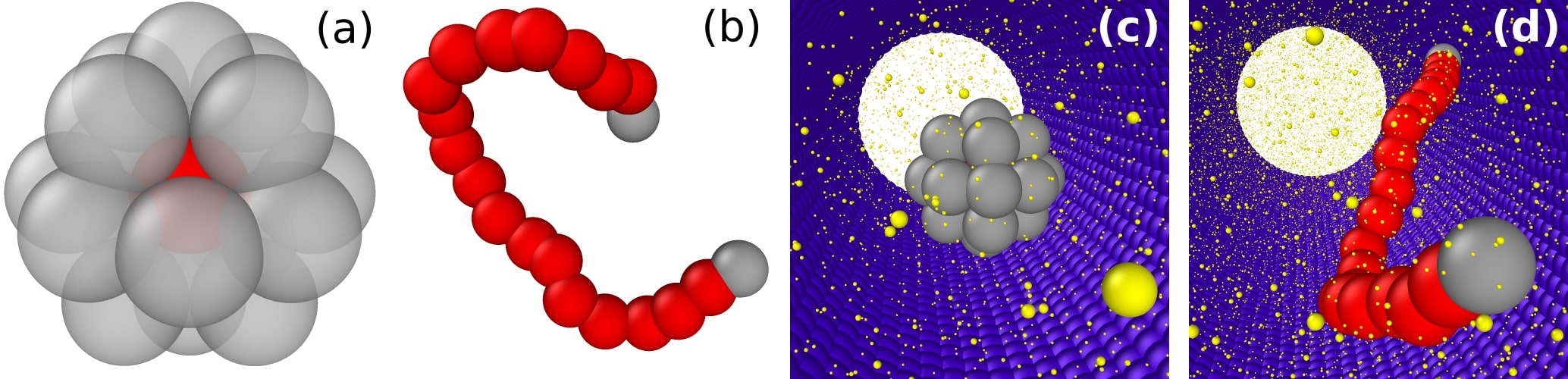
Figure 1: a: A raspberry-like active colloid composed of 19 particles. b: An active polymer composed of 20 beads. c: An active colloids in a cylindrical confinement. d: An active polymer in a cylindrical confinement.Red: thruster particles. Gray: filler particles. Blue: wall particles composing the confining channel. Yellow: solvent particles.

The propulsion mechanism of the thruster particle will be explained in the next section, when detailing the implementation of the hydrodynamic interactions. The orientation of the colloid is defined by the “active axis” identified by three chosen co-linear particles. This axis is also the symmetry axis of the force field we will apply to the solvent, and thus will define the colloid’s direction of propulsion. All particles belonging to each colloid interact via DPD: 1) with the solvent, 2) with particles belonging to other colloids and 3) with particles building the channel. However, particles belonging to each colloid do not interact between them, except for the rigid interactions that keep them glued together. In table 1 we report the chosen DPD parameters for all interactions between particles: solvent-solvent, solvent-colloid, solvent-cylinder, colloid-colloid, colloid-cylinder.

	$SOL$-$SOL$	$SOL$-$COL$	$SOL$-$CYL$	$COL$ -$COL$	$COL$ -$CYL$
$A$	25.0	25.0	100.0	25.0	25.0
$\gamma$	4.5	4.5	4.5	4.5	4.5
$r_{c}$	1.0	2.0	1.0	2.0	2.0

Table 1: DPD parameters used to study a spherical colloidal squirmer for ($COL$) embedded in a solvent ($SOL$), in bulk or in a cylindrical confinement ($CYL$). All parameters are in reduced DPD units.

In Section 2.4 we will describe different squirmer models, such as pushers, pullers and neutral swimmers, each one characterised by a different velocity field in the surrounding fluid. In order to check whether the raspberry-like colloid reproduces the features of the different squirmers, we compute the velocity fields and compared them to those reported for the different squirmers in Ref.starkMPC .

Having studied the active colloid in bulk, we study its physical behaviour when confined in cylindrical environments of different radii. The cylinder is composed of DPD overlapping particles, properly aligned along the $x$ axis at given angles. Overlapped DPD particles are left out of the time integration and thus can be used to model a wall. Particles are first evenly distributed along a circumference in the $yz$-plane and then this circumference is repeated through the $x$-axis. The separation of the particles is chosen so that the roughness of the inner surface of the cylinder is the same along the angular and longitudinal directions. Periodic boundary condition (PBC) are applied along the longitudinal direction ($x$ axis). Particles’ interaction parameters are reported in table 1.

DPD interactions between cylinder particles have been switched off. Choosing DPD interactions for modelling the collisions with the channel allows us to maintain a large time step $\Delta t=10^{-2}$. Due to the softness of the DPD interactions, we have appropriately set the DPD parameters for the channel particles to avoid leaking of solvent particles through the channel wall.

Moreover, DPD enables adding a friction between the solvent and the channel wall. In our case, we have tested that for high enough values of $\gamma$ we are able to simulate Poiseuille flow. However, for our study we have decided to explore low values of $\gamma$: this corresponds to the implementation of slip boundary conditions at channel’s walls.

II.3 Polymers in bulk and in confinement

Following Ref. bianco , we model the active polymer as a chain of active monomers. As shown in fig. 1.b, each of the $N_{b}$ monomers is composed by a single thruster DPD particle, except the head and tail monomer. Monomers are held together to their first neighbours via an harmonic potential $V_{\rm{harmonic}}(r)=K(r-r_{0})^{2}$, acting between thruster particles of the connected beads separated by a distance $r$, with $K=30$ $k_{B}T/\sigma_{dpd}^{2}$, being $r_{0}\equiv 1.5\,\sigma_{dpd}$. Since all interaction between particles are soft (DPD-like), we can choose $dt=10^{-2}$ as a time step to integrate the equations of motion.

As in Ref.bianco , we assume that all monomers are active a part from the first and the last (in grey in fig. 1). An active force $\bf{F}_{a,i}$ acts on each thruster monomer ${\bf r}_{i}$: the force is characterised by a constant magnitude $F_{a}$ and a direction of ${\bf r}_{i+i}-{\bf r}_{i-i}$ parallel to the polymer backbone tangent, being ${\bf r}_{i+i}$ and ${\bf r}_{i-i}$ the position vectors of the thruster particles of neighbouring monomers.

To characterise the bulk properties of an active polymer, we study a dilute system of 4 active polymers in a box with edge $L=20$ at a solvent density of $\rho=3$. Care must be taken if the volume fraction of polymers is not low enough, since polymers might interact via hydrodynamics. This is not our case, since in our system the polymers volume fraction is always lower than 5%) simulations to avoid the interaction between polymers.

To study the polymer under confinement we embed the active polymer and the solvent in a cylindrical channel with periodic boundary conditions along the axial axis. The cylinder consists of $N_{c}=24415$ frozen WCA-like particles that interact with the DPD particles (solvent and polymers) via a WCA-like potential

$$V_{\rm LJ}(r)=\begin{cases}4\epsilon\left[\left(\frac{\sigma_{dpd}}{r}\right)^{12}-\left(\frac{\sigma_{dpd}}{r}\right)^{6}\right]+\epsilon;&{\text{for}}\,\,r<2^{1/6}\,\sigma_{dpd},\cr 0;&{\text{for}}\,\,r\geq 2^{1/6}\,\sigma_{dpd},\end{cases}$$ (2)

where $\epsilon$ is the unit of energy and $\sigma_{dpd}$ represent the monomer diameter. In all simulations we set $k_{B}T=1.0$ (Lennard-Jones units). Cylinder particles are located close enough to avoid DPD solvent particles to cross the cylinder’s wall.

The chosen values for the DPD parameters are reported in table 2 for all interactions between particles: solvent-solvent, solvent-polymer, solvent-cylinder, polymer-polymer, polymer-cylinder.

	$SOL$-$SOL$	$SOL$-$POL$	$SOL$-$CYL$	$POL$-$POL$	$POL$-$CYL$
$A$	25.0	25.0	25.0	25.0	0.0
$\gamma$	4.5	4.5	4.5	4.5	0.0
$r_{c}$	1.0	1.0	1.0	1.0	0.0
$\epsilon$	0.0	0.0	0.0	0.0	1.0

Table 2: DPD parameters used to study an active polymer ($POL$) embedded in a solvent ($SOL$), in bulk or in a cylindrical confinement ($CYL$). All parameters are in reduced DPD units.

We should stress the fact that when dealing with active colloids or active polymers we have chosen to simulate the cylindrical channel in a different way. In the former case, the channel has been simulated by means of particles interacting via DPD, as explained earlier when describing the simulation details for the active colloid. Whereas in the latter case, the channel has been built using particles interacting via a repulsive potential, to compare with Refbianco .

II.4 Swimming induced by hydrodynamics

In order to numerically consider full hydrodynamic interactions between the active agents and the surrounding solvent, we prescribe a force field for the solvent particles surrounding the thruster particles of the active agent (the red particles in fig. 1).

When dealing with a spherical squirmer, the usual approach consists in prescribing tangential velocities to the solvent particles at the swimmers surface lighthill . Note that we have not followed the usual squirmer approach. In our case, tangential solvent forces, instead of velocities, are prescribed over a hydrodynamic active volume $\Gamma_{H}$ around the colloid, instead of just at the colloid’s surface. This approach is more general since it enables the possibility of studying different agent shapes and inertial effects, which are present in many active systems lowen_inertial .

In this study we only consider axisymmetric force fields, choosing the hydrodynamic region $\Gamma_{H}$ as a spherical shell around the thruster particles of inner and outer radii $R_{c}$ and $R_{H}$, respectively. $\Gamma_{H}$ is the region where a redistribution of the force fields between solvent and thruster particles occurs. The expressions of the force fields considered for the colloid and the polymer are reported in what follows (see the appendix for more details).

$$\bm{f}(r,\theta)=\big{[}f_{r}(r,\theta)\bm{\hat{e}}_{r}+f_{\theta}(r,\theta)\bm{\hat{e}}_{\theta}\big{]}P_{R_{c},R_{H}}(r)\$$ (3)

where $r$ is the distance from the thruster to the solvent particle, $\theta$ the angle between the agents orientation and the solvent position vector $\vec{r}$, $\hat{e}_{r}$, $\hat{e}_{\theta}$ are radial and tangential unitary vectors with respect to the colloid frame of reference and $P_{R_{c},R_{H}}(r)=\Theta(r-R_{c})\Theta(R_{H}-r)$ is a pulse function in the radial dimension which implements the spherical shell.

In order to have more control over the propelling force, we normalize the force field over the hydrodynamic region $\Gamma_{H}$, and multiply by a factor $F_{p}$. $F_{p}$ is the input parameter for the magnitude of the self-propelling force. Thus the hydrodynamic force field that will be applied to the solvent reads,

$$\bm{f}_{H}(r,\theta)=F_{p}\frac{\bm{f}(r,\theta)}{N},\quad\text{where}\quad N=\left|\int_{\Gamma_{H}}\bm{f}(r,\theta)\,\text{d}V\right|.$$ (4)

Since in our case we are dealing with a discrete fluid (made of solvent particles), the $i$-th solvent particle will feel a force,

$$\bm{f}_{H}^{\,i}=F_{p}\frac{\bm{f}(r_{i},\theta_{i})}{N},\quad\text{where}\quad N=\bigg{|}\sum_{j\in\Gamma_{H}}\bm{f}(r_{j},\theta_{j})\,\Delta V\bigg{|}$$ (5)

where the sum is taken over all the solvent particles that are inside $\Gamma_{H}$ and $\Delta V=r_{c}^{3}=1$.

In case of a spherical colloidal particle only the first two surface modes of the polar component, $f_{\theta}(r,\theta)$, are considered and the radial component is neglected $f_{r}(r,\theta)=0$ (see appendix sec. V.1 for the details). Thus, the force field becomes,

$$\bm{f}(r,\theta)=(B_{1}\sin\theta+B_{2}\sin\theta\cos\theta)P_{R_{c},R_{H}}(r)\bm{\hat{e}}_{\theta}\equiv\bm{f}_{\text{col}},$$ (6)

for which $N=(R_{H}^{3}-R_{c}^{3})B_{1}\pi^{2}/4$. In this way, the total propulsion force (which is precisely the integral appearing in eq. 4) experimented by the colloid is just $F_{p}$. $B_{2}$ controls the asymmetric character of the force field. Because of this formulation, $B_{1}$ plays no role and will be fixed to $1.0$ from here on. As in the squirmer model, we define $\beta=B_{2}/B_{1}$ as the active stress parameter that controls the type of squirmer (see fig. 2). Under the assumption of Stokes flow (low Reynolds number), it is reasonable to think that the velocity field of the solvent particles will resemble that of the squirmer model starkMPC ; lighthill .

Now we need to deal with the reaction force that is exerted on the colloid which will result in its thrust. Moreover, since an active colloid is an extended rigid object we would like to preserve the torque that may arise due to density fluctuations or interactions with other agents or objects. The reaction thrust force ($\mathbf{f}_{T}$) is applied on the nearest colloid particle (thruster or not) to each of the solvent particles and it is equal and opposite ($-\mathbf{f}_{H}$) to the redistributed force on that solvent particle:

$$\bm{f}_{T}^{\,k}(r,\theta)=-\bm{f}_{H}^{\,i(k)}(r,\theta)$$ (7)

where $i(k)$ represents the nearest solvent particle to the $k$-th colloid particle.

At each step, we implement the following algorithm:

1. We identify the neighboring particles around the agent’s thruster particles located between the agent radius ($R_{\text{col}}$ for the colloid; $r_{c}$ for the polymer) and the “hydrodynamic” radius $R_{H}$.

2. We compute the force field $\bm{f}_{H}$ in Eq. (4) at each of the neighbors positions, consistently with the agents orientation. The norm of the total distributed force is also computed.

3. For each neighbor,

4. 1. we apply the corresponding normalized force;

   2. we find the nearest agent particle and apply the same and opposite force.

In this way self-propulsion is achieved, while linear and angular momenta are locally conserved at each step. This procedure enables physically realistic modeling of the propulsion mechanism of a wide range of self-propelled systems, both living and artificial.

In case of the active polymer, we have considered a constant field modulated by $\cos\left(\frac{\theta}{2}\right)$ for each thruster monomer,

$$\bm{f}(r,\theta)=-\cos\left(\frac{\theta}{2}\right)P_{R_{c},R_{H}}(r)\,\bm{\hat{e}}\equiv\bm{f}_{\text{pol}},$$ (8)

where $\bm{\hat{e}}=\cos\theta\,\bm{\hat{e}}_{r}-\sin\theta\,\bm{\hat{e}}_{\theta}$ is the self-propulsion direction of the thruster particle. In this case, a reaction force that provides thrust to the agent is applied on each thruster particle. This force is equal and opposite to the total force distributed among the solvent particles in each step. Since in this case we are dealing with a flexible object that has many thruster particles, we need not to worry about the reaction force, since this is already taken care of, as the force that each thruster particle redistributes is equal and opposite to the one that is exerted on it.

In figure 2 we can see the hydrodynamic force fields, $\bm{f}$, we have used in this work. The continuous and dashed circumferences represent the inner ($R_{c}$), and outer ($R_{H}$) radius respectively and define the region $\Gamma_{H}$ where redistribution occurs. In this figure the propulsion force is computed as the surface integral of the vector field inside this region, $\bm{F}_{p}=-\int_{\Gamma_{H}}\bm{f}_{H}(r,\theta)\,d\bm{S}$, in this case computed in 2D as an example. Since the force field is asymmetric there exists a net propulsion force that provides thrust to the agent. In the case of the polymer (d), each polymer bead (or monomer) acts as a small colloid with its own redistribution field, so in this case $R_{c}=r_{c}$ would represent the beads radius, i.e. the thickness of the polymer.

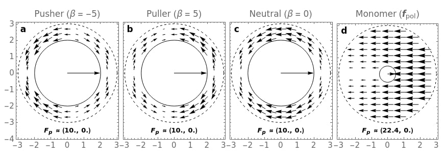
Figure 2: Examples of 2D hydrodynamic redistribution force fields for all the studied cases: a pusher (panel a) with $\beta=-5$, a puller (panel b) with $\beta=5$, a neutral squirmer (panel c) with $\beta=0$ and a monomer of the active polymer (panel d). These correspond to a section of the 3D field passing through the equator of the redistribution sphere. The arrow inside the central colloid indicates the direction of the propulsion force $F_{p}$, with magnitude indicated in each panel.

To conclude, the total force experienced by an agent particle consists of the following contributions

$$\bm{F}=\bm{F}_{C}+\bm{F}_{D}+\bm{F}_{R}+\bm{F}_{T}$$ (9)

where $\bm{F}_{T}$ is the total thrust force, computed as the sum of all the forces on each colloid particle $\bm{F}_{T}=\sum_{k}\bm{f}_{T}^{k}$. It is worth noting that while in this study we have restricted ourselves to axisymmetric force fields, the code implementation is made for general force fields, allowing for example azimuthal flows, like those of the Volvox algae Drescher2009 .

II.4.1 Quantifying activity

To characterise an active agent in the solvent, we will define adimensional numbers such as the Reynolds number and the Péclet number. For this, we will need to establish the viscosity $\eta$ of the fluid. $\eta$ can be numerically computed in a DPD fluid, as recently shown in Ref.Panoukidou2021 , or estimated via a mean field, as in Warren and Groot Groot . In our work, we follow the second approach, according to which the DPD solvent kinematic viscosity $\nu$, defined as $\frac{\eta}{\rho}$, can be computed as

$$\nu=\frac{\eta}{\rho}=\frac{D_{sol}}{2}+\frac{2\pi\gamma\rho r_{c}^{5}}{1575}$$ (10)

where the diffusion coefficient $D_{sol}$ is

$$D_{sol}=\frac{45k_{B}T}{2\pi\gamma\rho r_{c}^{3}}.$$ (11)

For more details, see Warren and Groot Groot . Note that in MPCD the viscosity can be computed as $\eta=16.05\,\sqrt{m_{0}k_{B}T}/a_{0}^{2}$, where $m_{0}$ and $a_{0}$ are the mass and the size of the cell used in MPCD algorithm. See StarkPeclet ; Noguchi2005 ; Kikuchi2003 ; Tuzel2003 for more details.

Once we know the viscosity, we compute the Reynolds number and the Péclet number. The Reynolds number quantifies the amount of inertial versus viscous forces acting on an object that moves in a fluid, cause by the different fluid velocities.

$$\text{Re}=\frac{v_{p}r_{c}}{\nu}$$ (12)

where $r_{c}=1$ is the solvent characteristic length and $v_{p}$ is the active agent’s propulsion velocity. For both the active colloids and the active polymer, the velocity is the one of the center of mass.

The Péclet number is defined to describe the degree of activity in the system as the ratio between the self-propulsion of the active agent and a persistent velocity scale $\mathrm{Pe}=v_{p}\,\tau_{r}/\sigma$. However, different works have shown different definitions for this number. We define the Péclet number for the colloid following Ref. StarkPeclet as,

$$\text{Pe}_{col}=\frac{v_{p}R_{\text{col}}}{D_{col}}$$ (13)

here $D_{col}=k_{B}T/6\pi\eta R_{col}$ is the diffusion coefficient of the colloid and $R_{\text{col}}$ is the colloid radius that if fixed to 2 for all our simulations with the exception of the flow fields shown in figure 3 in which $R_{\text{col}}=3$ was chosen for better visibility. We studied the following ranges $F_{p}\in[0,50]$, $v_{p}\in[0,1.25]$, $\mathrm{Pe}\in[0,156]$ and $\mathrm{Re}\in[0,12]$. As mentioned earlier, for some parameters we cannot assume that we are at Stokes flow conditions, so we should not use the relation $v_{p}=F_{p}\,/\,6\pi\eta R_{c}$ for computing the colloids propulsion velocity, this is why we “measure” it as $v_{p}=\langle\bm{v}_{\text{col}}\cdot\hat{\bm{e}}\rangle_{t}$. The values obtained are shown in fig. 10 of the appendix sec. V.2. Note that it was found that the propulsion velocityof the colloid, and thus the $\mathrm{Pe}$ and $\mathrm{Re}$, are not always linear with the propulsion force $F_{p}$. Moreover, they change whether we are dealing with pusher, neutral or puller squirmers, in fig. 10 we show the different propulsion velocities found (and their corresponding $\mathrm{Pe}$ and $\mathrm{Re}$) for each type of squirmer. However, in all simulations presented, we remain in the range $F_{p}\in[0,\,50]$ where the separation between the $v_{p}$ values for different squirmer types is not so dramatic and the behaviour does not depart too much from linearity.

For the polymer we follow the ref. bianco and define the Péclet number as

$$\text{Pe}_{pol}=\frac{F_{p}\cdot\sigma_{dpd}}{k_{B}T}$$ (14)

where $\sigma_{dpd}=1$ is the diameter of the monomers. The length of the polymer $N_{b}$ range between 40 and 100. For this particular cases we have explored values $\mathrm{Pe}=\{0.01,0.1,1.0\}$ that correspond with Reynolds numbers in the laminar regimen, around Re$\approx 0.3$.

II.5 Analysis tools

In order to characterise a system consisting of active agents in a solvent, we compute both structural and dynamical features. Concerning the active colloid, we first establish the velocity field of the solvent surrounding the swimmer to characterise the nature of each spherical squirmer (whether pusher, puller or neutral). Next, we study its dynamics by computing the mean square displacement, from the long time behaviour of which we could estimate the effective diffusion coefficient. Concerning the active polymer, we first characterise how activity affects its structural features by computing the radius of gyration. Next, we study its dynamics by computing the mean square displacement of the center of mass, from the long time behaviour of which we could estimate the effective diffusion coefficient.

Velocity fields. For computing the solvent velocity fields around the colloid we run simulations of a fixed colloid in the center of the box pointing to the positive $x$-axis. Then, we perform a binning of the simulation box and average the velocities of the solvent particles inside each bin, finally we also take ensemble and time averages in the stationary state. The velocity fields shown in fig. 3 correspond to a slab that has the same height as the colloid ($D_{\text{col}}$). The arrows represent the $xy$-projection of the full 3D velocities.

MSD. Concerning dynamical features, we compute the mean square displacement

$$\mathrm{MSD}(t)=\langle\,\left[\mathbf{r}_{\mathrm{cm}}(t)-\mathbf{r}_{\mathrm{cm}}(0)\right]^{2}\,\rangle$$ (15)

Where $\mathbf{r}_{\mathrm{cm}}$ indicates the position of the center of mass of the colloid/polymer. The average is taken over several colloids/polymers. The long time behaviour of the MSD, corresponds to the diffusion coefficient $D$, $\mathrm{MSD}(t)=6Dt$. It is worth noting that when confinement takes place in a cylinder with a small radius, it might be better to consider the system as one dimensional, thus $\mathrm{MSD}(t)=2Dt$. However, this is not our case since we consider that the agents have sufficient space to diffuse in the transverse directions. This leads to a more straighfoeward comparison between the different systems.

OACF The orientation autocorrelation function is also computed for the colloid in confinement to asses the impact of the confinement in the rotational diffusion (or equivalently, the reorientation time) of the colloid.

$$\mathrm{OACF}(\Delta t)=\frac{1}{N_{\Delta t}}\sum_{i=0}^{N_{\Delta t}}\hat{\bm{e}}(t_{i})\cdot\hat{\bm{e}}(t_{i}+\Delta t)$$ (16)

Here $\Delta t=n\,dt$ where $dt$ is our base time step. The scalar product of the orientation at a given time $\hat{\bm{e}}(t_{i})$ with itself at a delayed time $\hat{\bm{e}}(t_{i}+\Delta t)$ is averaged over the intervals of length $\Delta t$, starting at all the possible $t_{i}$’s, that fit into the total simulation time $T_{\mathrm{sim}}=N_{\mathrm{tot}}dt$. So there would be $N_{\Delta t}=N_{\mathrm{tot}}-n+1$ intervals of the same length in the full simulation interval for a given $n$.

RoG. The radius of gyration $R_{g}$ for the active polymer is computed according to the relation

$$R_{g}^{2}={\frac{1}{N}}\sum_{k=1}^{N}\left(\bf{r}_{k}-\bf{r}_{cm}\right)^{2},$$ (17)

where $\mathbf{r}_{\mathrm{\bf cm}}$ is the position of the center of mass of the polymer, $\mathbf{r}_{\mathrm{\bf k}}$ is position of the $k$ thruster particle and $N$ is the number of bead of the polymer

III Results

In what follows we present the results obtained for both active agents, either in bulk or in cylindrical confinement. We start with the simplest object: the spherical squirmer (Section 3.1) characterising its hydrodynamic features (Section 3.1.1) and its dynamical properties (Section 3.1.2). When confined in a cylindrical channel, we also compute its orientation autocorrelation function (Section 3.1.3). Next, we study the more complex-shape active polymer (Section 3.2), characterizing its structural (Section 3.2.1) and dynamical (Section 3.2.3) properties, compare our results with the passive and Brownian counterpart.

III.1 Active colloids

III.1.1 Flow Fields

To start with, we present our results for a spherical squirmer and study the velocity fields for the pusher, the puller, and the neutral swimmer.

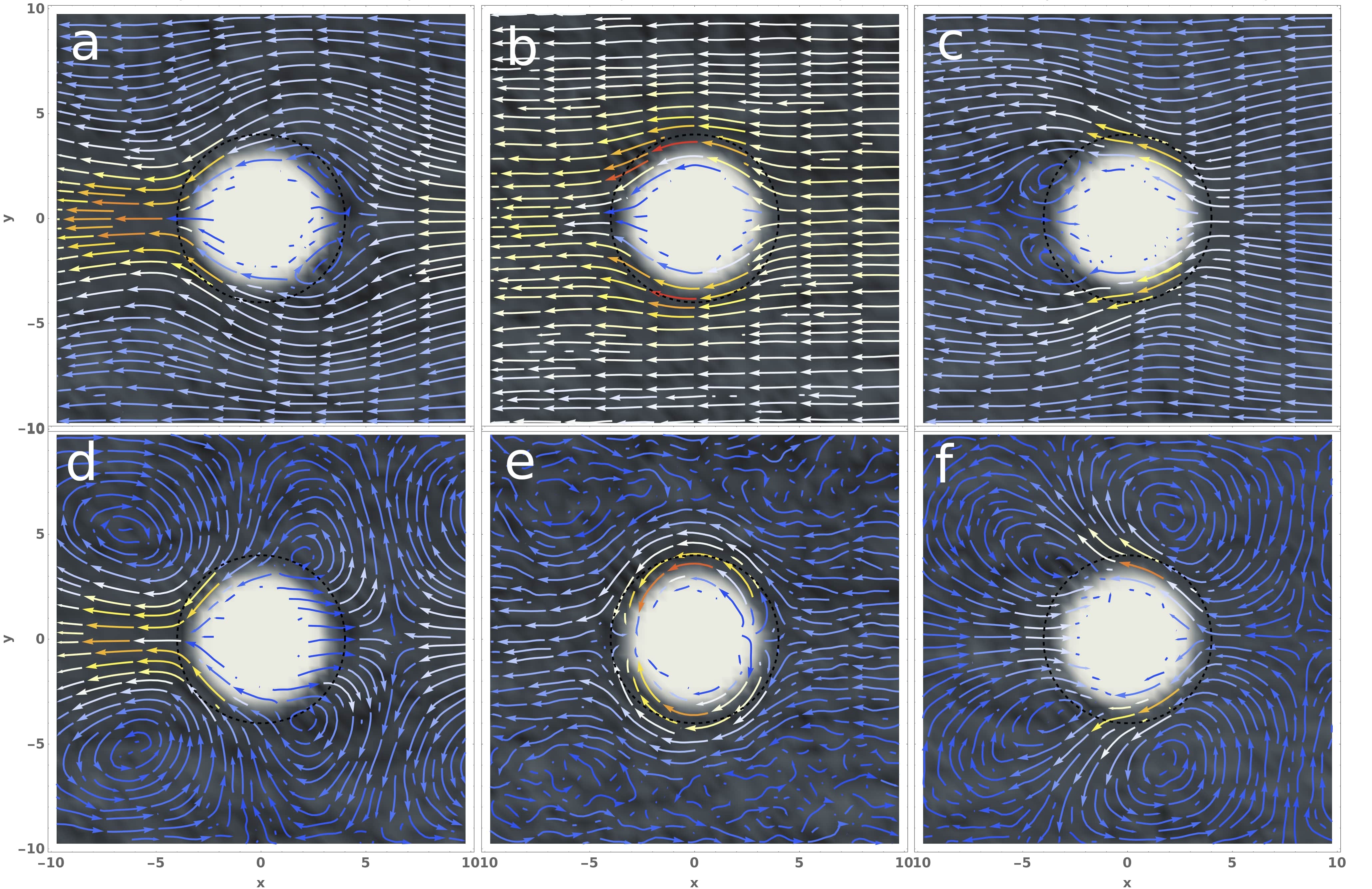
Figure 3: Sections of the velocity fields in the lab frame (bottom row) and moving with the colloid (top row), for the pusher (a, d), neutral (b, e) and puller (c, f) squirmer. surrounded by $\sim 10^{4}$ fluid particles and swimming to the right. The colour of the background is the averaged density of fluid particles, the colour of the arrows shows the fields magnitude. Here the colloid radius is $R_{c}=3$ and $F_{p}=100$ in order to obtain a clearer flow field. These values produce $\mathrm{Pe}\approx\{818,\,655,\,573\}$ and $\mathrm{Re}\approx\{25,\,20,\,17\}$ for the pusher, neutral and puller squirmers respectively.

In fig. 3 we present the velocity flow fields for this three squirmers computed as explained in the previous section: pusher (a, d), neutral (b, e) and puller (c, f) squirmer. Comparing our results with the typical flow fields expected for squirmers (e.g. ref. starkMPC ) the flow fields reported in Fig. 3 are not so symmetrical, in the case of the puller and pusher lab frames (figs. 3.d and 3.f). The four characteristic vortices of the flow field when periodic boundary conditions are present holmLBsquirmer seem to be shifted to the negative $x$-direction, compressing the two at the front and stretching the two at the back. In the same way, in the relative frame, we can see smaller swirls than usual at the front of the pusher (fig. 3a) and somewhat elongated ones at the back of the puller (fig. 3.c). In the case of the neutral swimmer, the characteristic source dipole of the lab frame (fig. 3.e) is completely compressed against the swimmers surface, and some turbulent flow is appreciated at the edges of the $y$-dimension of the section. All these deviations from the usual flow fields are ascribed to inertial effects of the fluid stemming from the high Reynolds number present in our simulations. In the Appendix V.3 we show the flow fields for a different set of parameters (lower Reynolds number, at $\mathrm{Re}\approx 0.1$) for which we find a more typical squirmer flow field starkMPC ; holmLBsquirmer .

Confining the colloid inside a cylindrical channel has a drastic impact in the solvent flow fields (fig. 4), since the channel walls change the boundary conditions of the fluid.

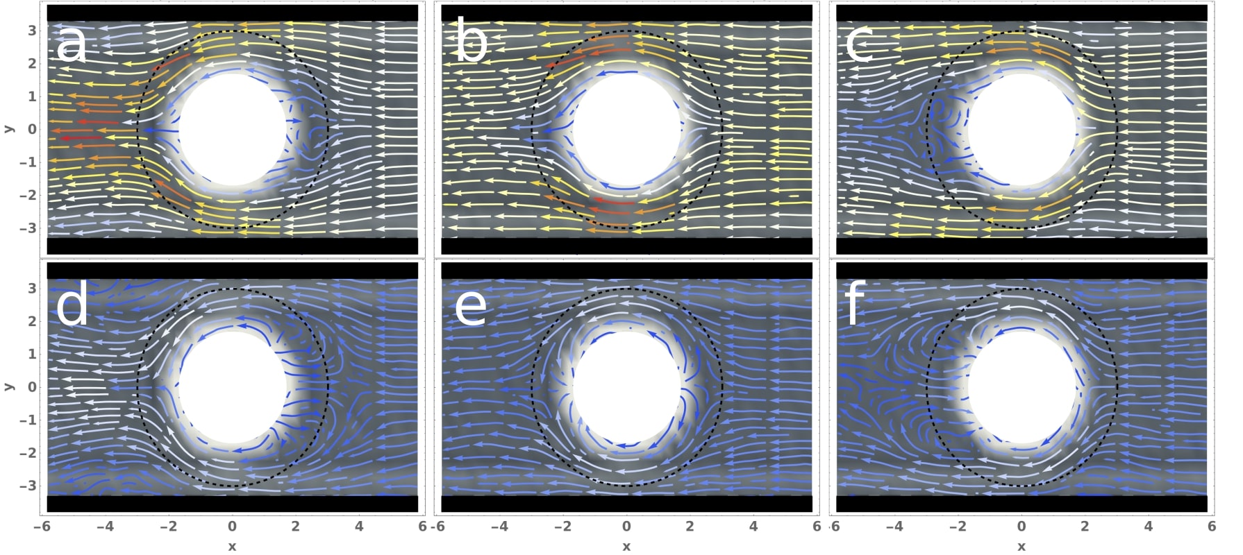
Figure 4: Solvent flow fields of the colloid confined in an cylindrical channel ($R_{\text{cyl}}=3.5$) in the lab frame (bottom row) and moving with the colloid (top row), for the pusher (a, d), neutral (b, e) and puller (c ,f) squirmer. Here the colloid radius is $R_{c}=2$ and $F_{p}=50$. These values produce $\mathrm{Pe}\approx\{90,\,76,\,61\}$ and $\mathrm{Re}\approx\{3.9,\,3.3,\,2.7\}$ for the pusher, neutral and puller squirmer respectively.

For the pusher and the puller in the absolute frame (figs. 4.a and 4.d) we observe that the two vortices at the back and front respectively seem to disappear, while the other two (at the front of the pusher and at the back of the puller) seem to have retracted to a closer position directly in front of the pusher and behind the puller. In the relative frame of reference, the swirls have also contracted further, and it is now difficult to distinguish them from just turbulent flow. It is surprising that in the case of the neutral swimmer (figs. 4.b and 4.e) the flow fields do not differ that much with respect to the ones encountered in bulk, with the exception that now there are no turbulent regions at the edges of the flow field.

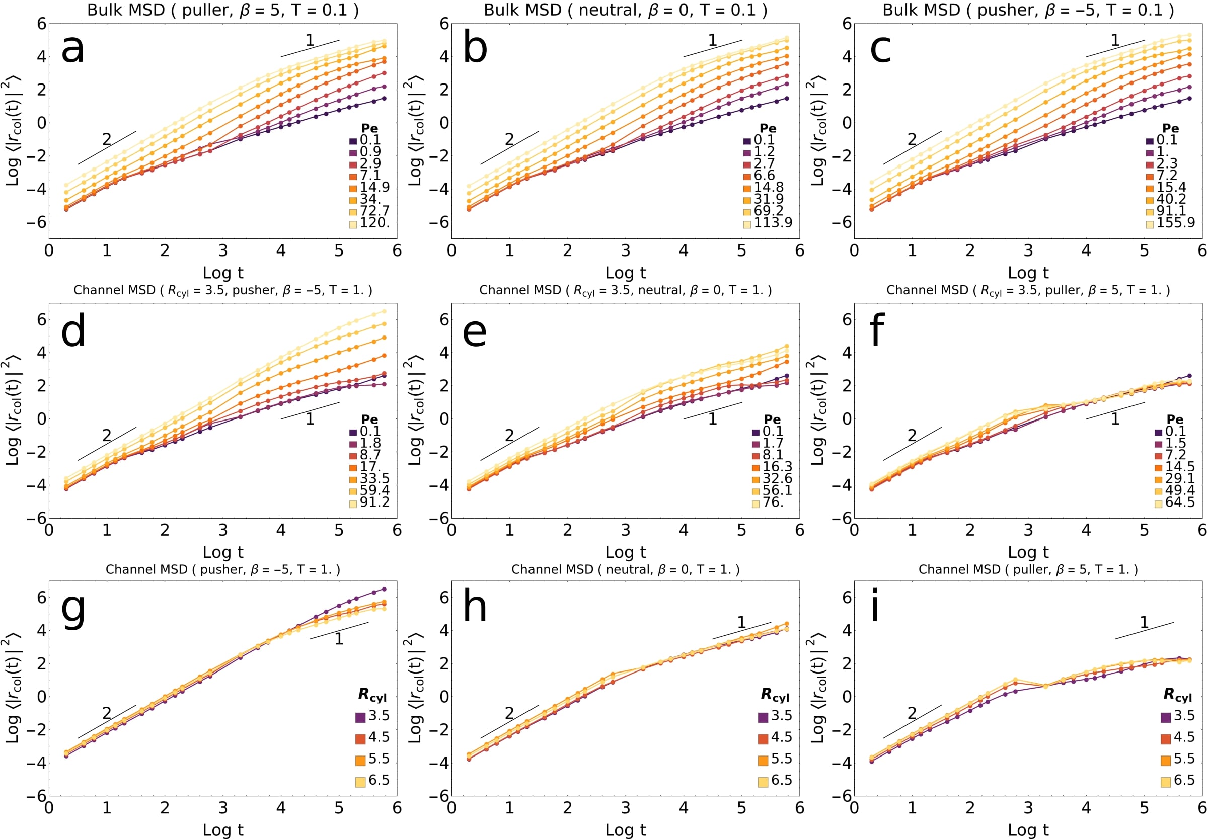
Figure 5: MSDs for the three squirmer types studied. Left column: pusher (panels a, d and g). Center column: neutral (panels b, e and h). Right column: puller (panels c, f and i). Top row: bulk (panels a, b and c). Center row: in cylindrical confinement for different $\mathrm{Pe}$’s for the smallest channel radius $R_{\text{cyl}}=3.5$ (panels d, e and f). Bottom row: for different channel radii for the highest Péclet numbers available corresponding to the highest thrust force $F_{p}=50$ (panels g, h and i).

III.1.2 Diffusion

When dealing with a colloidal squirmer in bulk, we study its dynamical features by estimating the long time diffusion coefficient normalised by the diffusion of a passive colloid in bulk via the center of mass mean square displacement, as explained in Section 2.5., for the three types of squirmers (figs. 5a-c).

The top row of panels in fig. 5 represent the MSD for a bulk dilute suspension of pushers (a), neutrals (b) and pullers (c). Their long time behaviour corresponds to the diffusion coefficient reported in fig. 6.a From the results presented, it is reasonable to conclude that the three types of squirmer diffuse almost the same for the ranges of Péclet numbers studied. As expected, the diffusion of the three of them increases when increasing their thrust force and thus their Péclet number. In fig. 6.a it is worth noting that as we increase the thrust force and thus the Péclet and Reynolds numbers, the diffusion behavior changes significantly, when we are in the range of $\mathrm{Re}\ll 1$ the diffusion increases significantly while we increase the $\mathrm{Pe}$, when we approach $\mathrm{Re}\approx 1$ the increase in diffusion is dampened reaching what seems to be a saturation as $\mathrm{Re}\gg 1$.

The middle and bottom row of panels in fig. 5 represent the MSD for a confined dilute suspension of pushers (a), neutrals (b) and pullers (c). The middle panels study the dynamics of swimmers in a channel with the smallest radius, while varying the Peclet number for pushers (d), neutrals (e) and pullers (f). The bottom panels study the dynamics of swimmers at the highest Peclet in a channel with varying radius for pushers (g), neutrals (h) and pullers (i). When we confine the active colloid inside a cylindrical channel the symmetry between pushers and pullers is lost. On the one side, if the puller encounters a wall it is more prone to get stuck since its thrust mainly comes from its front. Thus, due to the lack of solvent between the colloid and the wall the colloid experiments a torque that forces it to face the wall. On the other side, since pushers achieve their self-propulsion mainly as a thrust on their back part, they are less prone to get stuck when hitting a wall, experimenting a bouncing from it. This is in agreement with the MSD (figs. 5d-f) and also with previous literature Lauga_2009 ; starkMPC .

The same information will be recovered when plotting the OACF for each system (as will be shown in figs. 7e-g) curves).

As shown in the MSD curves (figs. 5d-f), for the pusher we detect a slight increase at large times, while for the puller the curves collapse showing a significant decrease in its motility at large times for all studied Péclet numbers . This is due to the wall-facing effect described previously, which is consistent not only with the decrease of motility, but also with the apparent independence of the diffusion with the Péclet number. The shape of the MSDs curves for the neutral swimmer (fig. 5e) also follow from this argument. The neutral squirmer gains its thrust force symmetricaly between its front and back. Therefore, it propels on its front more than the pusher but less than the puller, and propels on its back more than the puller but less than the pusher. The fact that this system is between the two is confirmed by the MSDs curves. The diffusion curves (fig. 6 a,b,c) show more clearly what we have just addressed.

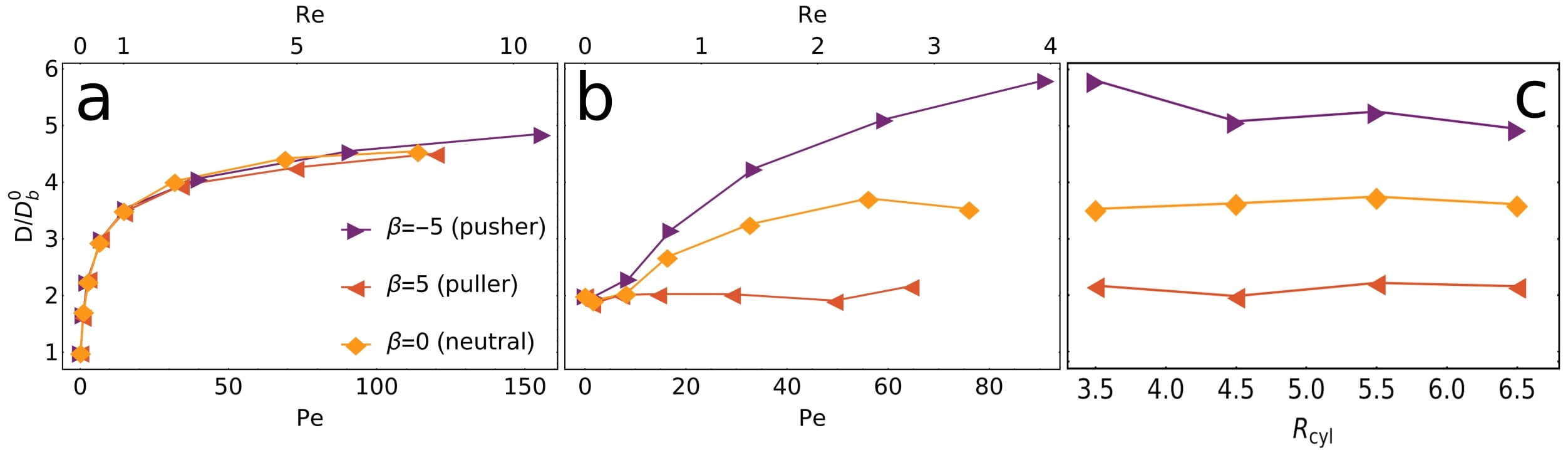
Figure 6: Diffusion as a function of the Péclet number for the active colloid in bulk (a), in confinement for the narrowest channel $R_{\text{cyl}}=3.5$ (b) and as a function of the cylinder radius for the highest Péclets (c) for the three squirmer types studied. We normalize by the diffusion of a passive colloid in bulk $D_{b}^{0}=0.032179$. In the two first plots a secondary horizontal axis shows the corresponding Reynols number.

In fig. 6c we report the normalized diffusion for highest Péclet number of the three types of squirmers in confinement as a function of the channel radius. The major effect of varying the channel radius occurs for the pusher, while the puller and neutral squirmer’s diffusion seems to remain unaffected by it (in the studied range). This is coherent with the wall-facing argument previously described. The diffusion is a long time property, while for the studied radii the colloid reaches the channel wall at much shorter time scales. Therefore once the colloid has reached the wall, it might get stuck due to the wall-facing effect regardless of the channels radius.

III.1.3 Orientation aturocorrelation function

Finally, we compute the orientation auto-correlation function (OACF) when active colloids are confined in a cylindrical channel, as depicted in fig. 7. The OACF measures the rotational diffusion (or equivalently, the reorientation time) of a colloid, i.e. for how long the colloid retains its swimming direction before it is randomized by fluctuations.

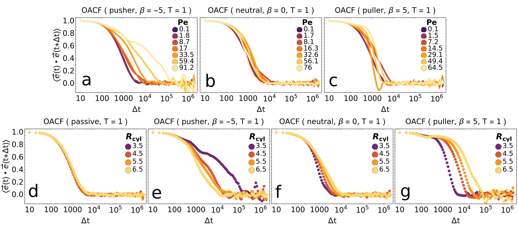
Figure 7: Auto-correlation function for the colloids orientation vector. Top: for the smallest cylinder radius $R_{\text{cyl}}=3.5$ and all the Péclet numbers studied for pusher (a), neutral (b) and puller (c). Bottom: for all the studied cylinder radii for a passive colloid (d)for which $F_{p}=0$, $\mathrm{Pe}=0.1\approx 0$ and the highest Péclet numbers available (all corresponding to $F_{p}=50$) for the three types of squirmers: pusher (e), puller (f) and neutral (g).

The top row of fig. 7 represents the OACF for the system confined in the smallest cylinder, when varying the Peclet number. Whereas the bottom row represents the OACF for an active colloid propelling at the highest Peclet number and confined in cylinders with different radii. In the case of a pusher (fig. 7a) we detect a clear increase of the reorientation time with increasing $\mathrm{Pe}$. This is expected for any non-chiral active particle which increases its $\mathrm{Pe}$ by increasing its propulsion force joseJCP Moreover, due to the wall-rebound argument discussed previously, this effect could be amplified. When dealing with the neutral (fig. 7b) and the puller (fig. 7c) squirmers, the interpretation is less clear. It seems that in both cases starting from the lowest $\mathrm{Pe}$ the reorientation time increases until it reaches a point where the behaviours for both squirmers is different. For the neutral squirmer, as we keep increasing $\mathrm{Pe}$ the reorientation time decreases, reaching a minimum for the highest $\mathrm{Pe}$. Whereas for the puller, at $\mathrm{Pe}=14.5$ there is a sharp decrease and then, as we keep increasing $\mathrm{Pe}$, a slight recovery. Anyhow it is hard to draw solid conclusions in both cases. One reason could also be due to not enough statistics.

Figure 7d-g offers a much clearer interpretation. In these panels we show how the OACF changes as we vary the channel radius keeping in all cases the maximum $\mathrm{Pe}$ available, corresponding to the highest thrust force $P_{p}=50$. As expected for a passive colloid (fig. 7.d) the OACF is the same regardless of the channel radius. Moving now to the pusher (fig. 7.e) we notice an increase of the reorientation time as we decrease the channel radius, consistent with the wall-rebound argument. For the puller (fig. 7.g) we encounter the opposite behaviour, the reorientation time increases with increasing radius, this can be explained with the wall-facing argument plus the fact that when the puller is swimming against the wall it is in an unstable state, similar to when a pencil is left standing at its tip, so it will change its orientation, some times this reorientation will lead him back to the center of the channel, but the narrower the channel, the sooner it will encounter again the wall and reorient again. For the neutral squirmer (fig. 7.f) we are again in between pushers and pullers but since neutrals propel slight in their front side, as pullers, the behaviour observed is more similar to pullers than to pushers.

III.2 Active polymer

In this section we present our results on structural and dynamical features of the active polymer in an explicit solvent. In particular, we focus on the radius of gyration $R_{g}$, and on the diffusion coefficient $D$, computed via the long-time behaviour of the mean square displacement of the polymer’s center of mass. We consider the active polymer first in bulk and then confined in a cylindrical channel, underlying the effect of the activity in comparison with the passive polymer behaviour in the same conditions. When in bulk, we unravel the effect of hydrodynamics comparing our results to the results obtained in Ref.bianco for Active Brownian polymers (without hydrodynamics).

III.2.1 Radius of Gyration

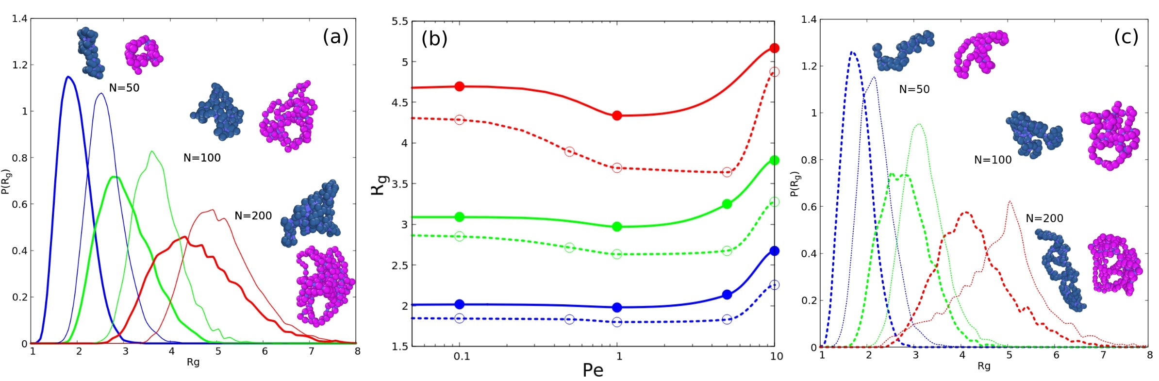
Figure 8: Probability distribution of the radius of gyration for passive ($\mathrm{Pe}=0$, thick line) and active ($\mathrm{Pe}=10$, thin line) polymers of N=50 (blue), N=100 (green), N=200 (red) monomers in bulk (a) and in confinement (c). The snapshots illustrate typical conformations for the passive (blue) or active (magenta) polymers. (b) Average value of $R_{g}$ as function of $\mathrm{Pe}$ for different polymer sizes. Continuous lines are for the polymer in bulk and dashed lines for the polymer under confinement.

Figure 8 a and c shows the probability distribution function of the radius of gyration for the polymer in bulk (panel a, continuous lines) and confined in a channel (panel c, dashed lines), comparing the passive (thick lines) to the active (thin lines) case. We also sketch snapshots representing typical conformations observed in each case, both for the passive case (in blue) and for the active one (in magenta). Panel b represents the average radious of gyration as a function of the Péclet number for polymer length of N=50 (blue), N=100 (green) and N=200 (red) in bulk (continous line) and in a channel (dashed line).

When studying a passive polymer in bulk (thick lines in fig. 8.a), our model recovers the expected increase of the radius of gyration with the polymer size. This behaviour is observed also in the presence of active forces as shown by the thin lines in fig. 8.a. In order to underline the relevance of hydrodynamics it would be interesting to compare the results obtained for the active polymer with those for the Active Brownian Polymer reported in Refbianco . However, a direct comparison is not possible, due to the different features of the chosen polymer’s model. In Refbianco the authors used a bead-spring self-avoiding polymer, whereas in our study we have used an ideal polymer.

When studying the average of the radius of gyration as a function of the Péclet number (fig. 8-panel b) we detect a non-monotonic behaviour. For short polymers ($N=50$), $R_{g}$ remains constant at low activities (until $\mathrm{Pe}=5$): the same behaviour has been detected in Ref.bianco for active Brownian polymers, sign that hydrodynamics is not relevant for low activities. For relatively short polymers ($N=50$ and $100$) the radius of gyrations is almost constant when activity is low activity, and increases at high activity. This behaviour corresponds to what one would expect if the polymer behaves like a flexible polymer.Das2021 However, when activity increases, the presence of hydrodynamics affects the polymer conformation since $R_{g}$ increases. On the other side, without hydrodynamics $R_{g}$ decreases. For larger polymers ($N>50$) $R_{g}$ reaches a minimum value before increasing again. The same behaviour have been already reported in Ref. Das2021 for active fully flexible Brownian self-avoiding polymer. Larger polymers ($N>200$) behave like a semi-flexible polymer Das2021 , characterised by an initial decrease of $R_{g}$ (more compact shape) for small values of the Péclet number, leading to an increase of $R_{g}$ with the activity (more open shape). This non-monotonic behaviour resembles the behaviour observed for the end-to-end distance of active polymers in the presence of hydrodynamicswinkler2020physics ; eisenstecken2016conformational .

Even when an active polymer is confined in a cylindrical channel (fig. 8.c), activity plays the same role on the probability distribution of the radius of gyration. The radius of gyration increases with the number of monomers $N$ when hydrodynamics is taken into account. This is expected, as we increase the mass of a polymer. Moreover, comparing the active (thin) to the passive (thick) polymer, the increase is more stretched in the active than in the passive case. Interestingly, the confinement does not seem to affect $R_{g}$ since same size active polymers ($50\leq N\leq 200$) are characterised by the same radius of gyration when in bulk or in a channel. Probably, the reason for this is that we have chosen to study a channel whose diameter is relatively large, thus not differing too much from the bulk system.

III.2.2 Diffusion

In order to understand the dynamical features of an active polymer in bulk and in confinement, we compute the MSD of the active polymer’s center of mass. As in Ref.bianco for the system without hydrodynamics and like the squirmers studied in the previous section, MSD present at short time a ballistic regime ($MSD\propto t^{2}$), a diffusive dependence at long time ($MSD\propto t$) and for middle times there is a crossover characterize for a super-diffusive regime ($MSD\propto t^{\nu}$, with $1<\nu<2$). From the MSD long time dependence, we estimate the diffusion coefficient. Figure 9 represents the diffusion coefficient $D_{eff}$ of the polymer’s center of mass as a function of the polymer size, when varying the Péclet number. While in panel a we have normalised the diffusion coefficient by the diffusion coefficient of the passive polymer ($D_{0}$), in panel b we have normalised the diffusion coefficient by the mean field diffusion of a DPD solvent particle ($D_{sol}$ in eq.22).

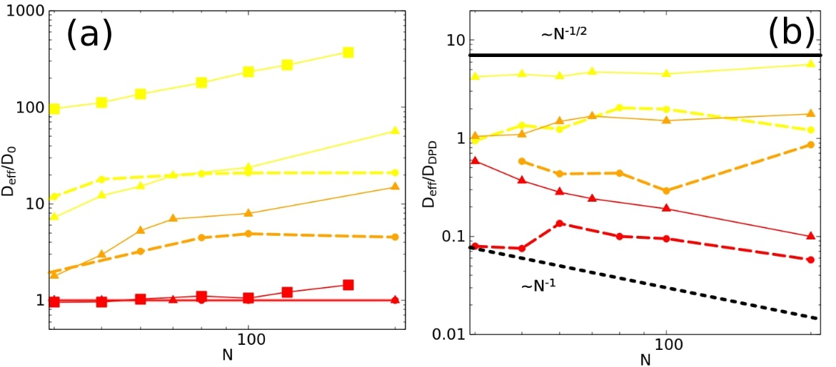
Figure 9: Diffusion coefficient of the polymer center of mass $D_{eff}$ as a function of the polymer length for three different Pe values 0 (red), 0.1 (orange) and 1 (yellow). (a) Normalised by the diffusion coefficient of the passive polymer ($D_{0}$); (b) normalised by the mean field diffusion of a DPD solvent particle Eq. (11). Square dots are results from Ref. bianco with permission of the authors, triangles are results for the system in bulk and circles for system in confinement.

In fig. 9.a. we show the results for the effective diffusion normalized by the diffusion coefficient of the passive case ($D_{0}$) as a function of the polymer size. We study values of activity ranging from the passive case (in red) to $Pe=1$ (yellow case) and observe that activity increases the effective polymer diffusion. Meanwhile, if we compare the Brownian diffusion bianco (yellow square) for the same activity $\mathrm{Pe}=1.0$ with our results (yellow triangles) we detect the same dependence with $N$ but approximately 10 times smaller. The effect of hydrodynamics is to slow down the polymers’ motion, as expected. Finally, if we compare the results obtained for the bulk system with the ones for the channel we observe how confinement does not seem to affect the small polymers ($N<50$), but turns out to be relevant when the length of the polymer is increased. For longer polymers ($N>70$) the confinement affects the polymer’s motion and the diffusion decreases when the polymer is too long.

On the other hand, in fig. 9.b. the effective diffusion has been normalized by the mean-field bead diffusion given by Eq. 11. The idea to represent the data in this way was to be able to establish a power law dependence of the diffusion coefficient with the polymer size and compare it with the prediction expected for the diffusion by the Rouse and Zimm zimm1956dynamics theory of Gaussian chains. Within this theory, the chain center of mass diffusion $D_{Rouse}\propto N^{-1}$ and $D_{Zimm}\propto N^{-1/2}$. As shown in figure 9.b, when the polymer is passive (red line), the power law resembles that predicted by the Rouse model, which does not take into account the hydrodynamic interactions between the beads of the polymer. While when the activity is relatively high (yellow line) the behavior is similar to that expected in the Zimm model, in which the hydrodynamic interaction between the polymer beads is not negligible, as expected.

IV Discussion

In many paradigmatic examples of active matter such as biological microswimmers or synthetic active colloids, the active agents are typically immersed in a solvent and the hydrodynamic interactions produced by the movement of the particles are relevant. Usually the introduction of these hydrodynamic interactions in active systems has been carried out through lattice models such as LB, that consider hydrodynamic effects but neglect thermal fluctuations, or event driven models such as MPCD that allow for the study of systems at low Reynolds number. In this work we start from a different point of view, developing a new methodology for the introduction of hydrodynamic interactions in mesoscopic molecular dynamics simulations. To do so, we have used the well known DPD model that has been showed to be a simple and well behaved coarse-grain model (for an specific set of parameters) for the implementation of hydrodynamics interactions in passive systems.

One of the main advantages of this new implementation is the possibility of easily taking into account thermal fluctuations for swimmers of complex shapes. Moreover, as our implementation has been developed as an adds on of the LAMMPSs open source package and will be sent to the LAMMPS developers (constantly maintaing the code). This makes our numerical approach readily available to be used.

In active systems there are a plethora of different mechanisms that produce the propulsion of the active agents, such as beating of flagella or chemical reactions. In our approach, we focus on the fact that in all these cases, the agents exert a force on the solvent in which they are immersed in order to achieve thrust. Depending on the type of propulsion mechanism employed, the exerted force has its own distinct features but it always respects the conservation laws of the different physical quantities. The model and its implementation is described in details, based mainly on momentum conservation: this corresponds to the fact that the force experienced by the active agent in its propulsion must be compensated by the stresses induced in the solvent.

To verify the validity of our model, we study two particular cases whose phenomenology has been well characterised by other numerical methods. The first of these cases are spherical squirmers, which represent the simplest model of an active agent in which the hydrodynamics of the system is taken into account. The second example studied is an active polymer, which is nothing more than a first approximation to a slightly more complex structure: a chain of swimmers. In this case, our proposed method is applied in the same way for each of the monomers (swimmers) that form the polymer. As shown in the results section, the proposed method leads to a phenomenology, such as flow fields, dynamical and structural features, consistent with the results obtained for the same systems studied with different numerical models.

Concerning the active colloid, we have been able to reproduce the solvent flow fields for the different types of swimmers (fig. 3), observing a characteristic deformation of the solvent flow fields due to the inertial effects present in the fluid at moderate Reynolds numbers $\mathrm{Re}\sim 20$. We have been able to asses the impact of these inertial effects on the dynamics and hydrodynamics of the swimmer and to conclude that pushers are the most efficient swimmers (in the sense that they develop a larger propulsion velocity for the same propulsion force, fig. 10), followed by neutrals and pullers when the Reynolds number is increased enough. For the ranges studied in the main part of our work, we showed that when swimming in bulk, diffusion is hardly affected by the choice of squirmer type (fig. 6a), and begins to saturate as we venture into higher Reynolds numbers. When the swimmer is confined inside a cylindrical channel, the flow fields changed dramatically in order for the fluid to adapt to the new boundary conditions (fig. 4). The confined geometry breaks this symmetry in the diffusion between the squirmer types (fig. 6b), as the behaviour of each swimmer near the channel wall is completely different: while pushers tend to rebound, aligning parallel to the wall and thus increasing their diffusion, pullers tend to get stuck, aligning perpendicularly with the wall and thus drastically decreasing their diffusion. Neutral squirmers lay in between both behaviours, but closer to pullers, as they slightly rely on the solvent ahead of them for achieving thrust. When varying the radius of the confining channel, diffusion of neutrals and pullers was hardly affected, while pushers enhanced their diffusion with decreasing channel radius (fig. 6c). Finally, we discussed the effect of the confinement in the reorientation time of the swimmers (fig. 7). We showed that pushers have slower reorientation dynamics the larger the Péclet number, but could not conclude anything solid for neutrals and pullers. Although when the Péclet is the highest and we increase the channel radius, the reorientation behaviour of pushers and pullers is clearly opposite: pushers increase their reorientation time while pullers decrease it. Again, neutrals lay in-between both behaviours although a little closer to pullers than to pushers.

In the active polymer case, we have compared the radius of gyration $R_{g}$ and diffusion to the system without hydrodynamics (Active Brownian Polymer). Concerning the radius of gyration $R_{g}$, the behavior of the polymer has been characterised as a function of both the polymer length and the Péclet number. Even though the radius of gyration monotonically increases with the polymer length (fig. 8), the dependence with the activity is not so straightforward. For short polymers $R_{g}$ always increases with activity, whereas for long polymers it reaches a minimum value. This behaviour has been already detected in active fully flexible Brownian self-avoiding polymers. On the other hand, confinement always decreases $R_{g}$ with respect to the system in bulk. When studying the dynamics of the polymer, we have compared our results with the analytical results for the Rouse and Zimm models, and concluded that our model (for the set of parameters used) is compatible with the prediction of the Rouse model at low Peclet (when hydrodynamics does not seem to play a relevant role), and is compatible to the Zimm model at higher Peclet number, when the monomers of the polymer chain can interact with each others due to hydrodynamics.

Having characterised the behaviour of individual swimmers in a solvent, we plan to use our numerical tool to study more dense suspensions of active colloids or active polymers. This will allow us to study their collective behaviour, their aggregation (if present) and the interplay played by hydrodynamics and activity, with the idea of comparing our numerical results on experiments on active synthetic colloids or active living swimmers (such as algae or bacteria), where hydrodynamics is relevant.

V Appendix

V.1 Detail on the hydrodynamic propulsion field

The radial and angular functions $f_{r}$ and $f_{\theta}$ can be expanded in terms of Legendre polynomials in a similar way than in the squirmer model, with the caveat that now we redistribute the forces on a spherical shell between $R_{c}$ and $R_{H}$ rather than just in the surface of the sphere,

$$f_{r}(r,\theta) =P_{R_{c},R_{H}}(r)\cdot\sum_{n}A_{n}P_{n}(\cos\theta)$$ (18)

$$f_{\theta}(r,\theta) =P_{R_{c},R_{H}}(r)\cdot\sum_{n}B_{n}V_{n}(\cos\theta)\quad$$ (19)

where

$$V_{n}(\cos\theta)=\frac{2\sin\theta}{n(n+1)}\frac{dP_{n}(\cos\theta)}{d\cos\theta}$$ (20)

and $P_{R_{c},R_{H}}(r)=\Theta(r-R_{c})\Theta(R_{H}-r)$ is a pulse function in the radial dimension which defines the spherical shell.

Truncating the series for $n>2$ we arrive at,

$$f_{r}(r,\theta) =\left[A_{0}+A_{1}\cos\theta+\frac{A_{2}}{2}(3\cos^{2}\theta-1)\right]\cdot P_{R_{c},R_{H}}(r)$$ (21)

$$f_{\theta}(r,\theta) =\left(B_{1}\sin\theta+B_{2}\sin\theta\cos\theta\right)\cdot P_{R_{c},R_{H}}(r)$$ (22)

V.2 Propulsion velocity

In Figure 10 we show the measured propulsion velocity of the colloid, $v_{p}=\langle\vec{v}\cdot\hat{e}\rangle_{t}$ with the corresponded Péclet and Reynolds numbers computed from eqs. 13 and 12, as a function of the propulsion force $F_{p}$ applied.

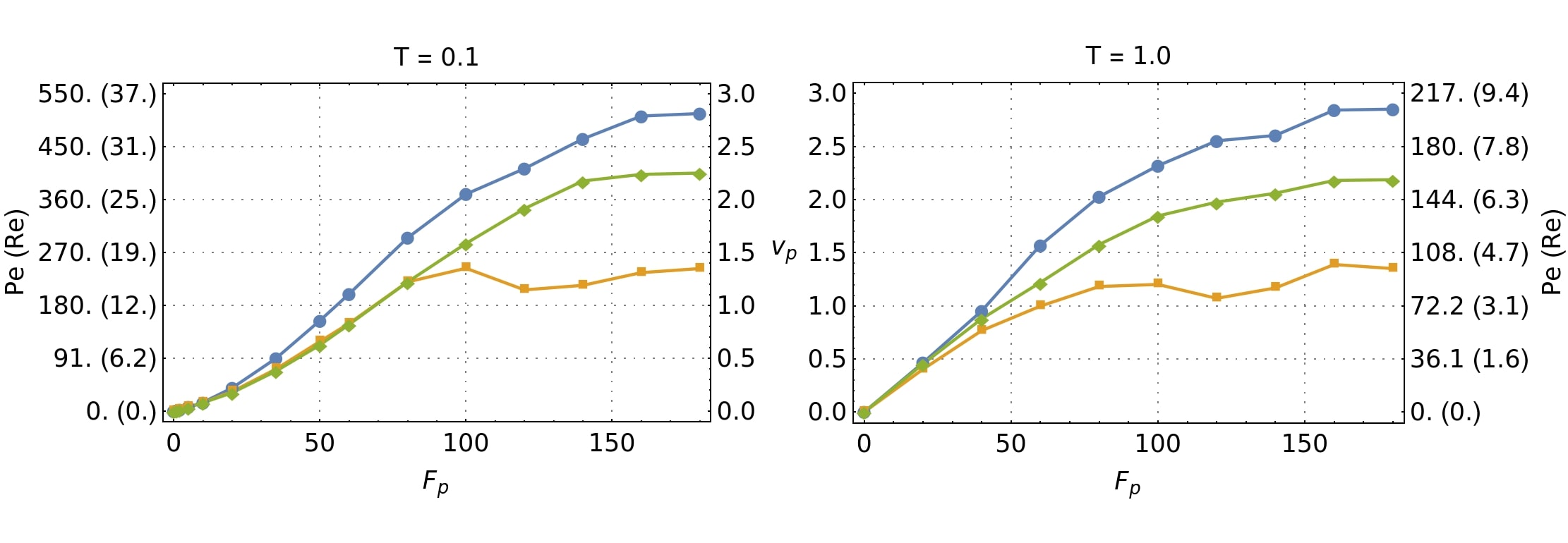
Figure 10: Propulsion velocity with its corresponding Péclet and Reynolds numbers as a function of the propulsion force of the colloid for the pusher (circles), neutral (diamonds) and puller (squares) squirmers, for $T=0.1$ (left) and $T=1.0$ (right). Note that for better readability, the right vertical axis of the left plot is shared with the left axis of the right plot and represents the propulsion velocity. The exterior axes represent the Péclet number and Reynolds number (between parenthesis) corresponding to each propulsion velocity.

As it can be seen the propulsion velocity is not linear with the propulsion force nor is the same for different kinds of squirmers. This maybe due to the fact that we are not at sufficiently low Reynolds number, since for low enough $\mathrm{Re}$ we notice that not only the relation is more linear but also that the curves collapse, giving almost the same values for the three types of squirmers. As a side result we can say that the pusher is the most efficient swimmer in this kind of environments, followed by the neutral and the puller squirmer.

V.3 Low Reynolds number

To verify that the deformation observed in the flow fields was indeed due to a high Reynolds number, we simulate a pusher in the same conditions as before but with a higher DPD friction coefficient ($\gamma^{ss}=270$) between the solvent particles. The resulting flow field (fig. 11) is less distorted, i.e. is more symmetric and the saddle point at the front of the pusher is closer to the edge of the simulation box, where it should be ideally.

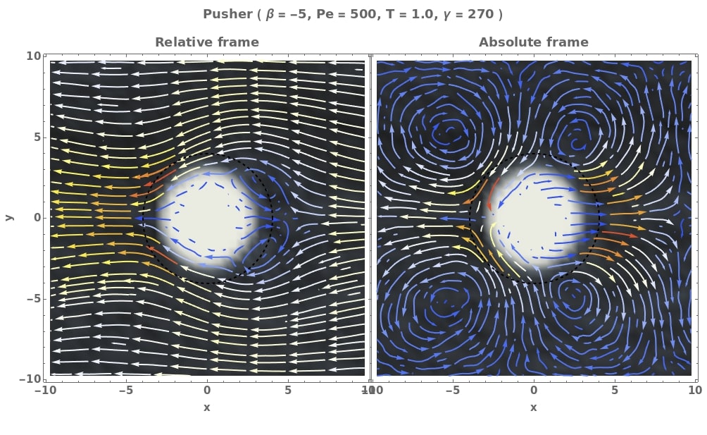
Figure 11: Pusher swimming to the right with $v_{p}\approx 0.4$, $\nu\approx 3.236$, $\mathrm{Re}\approx 0.1236$, $\mathrm{Pe}\approx 659.58$. Here we can achieve this lower Reynolds number because we choose the friction coefficient of the DPD solvent as $\gamma^{ss}=270$. Left: frame moving with the colloid. Right: lab frame.

References

- (1) G. Gompper, R. G. Winkler, T. Speck, A. Solon, C. Nardini, F. Peruani, H. Löwen, R. Golestanian, U. B. Kaupp, L. Alvarez, et al., “The 2020 motile active matter roadmap,” Journal of Physics: Condensed Matter, vol. 32, no. 19, p. 193001, 2020.
- (2) I. S. Aranson, “Active colloids,” Physics-Uspekhi, vol. 56, no. 1, p. 79, 2013.
- (3) A. Zöttl and H. Stark, “Emergent behavior in active colloids,” Journal of Physics: Condensed Matter, vol. 28, no. 25, p. 253001, 2016.
- (4) M. De Corato, X. Arqué, T. Patino, M. Arroyo, S. Sánchez, and I. Pagonabarraga, “Self-propulsion of active colloids via ion release: Theory and experiments,” Physical review letters, vol. 124, no. 10, p. 108001, 2020.
- (5) A. Lucia and E. Guzmán, “Emulsions containing essential oils, their components or volatile semiochemicals as promising tools for insect pest and pathogen management,” Advances in Colloid and Interface Science, vol. 287, p. 102330, 2021.
- (6) S. Ebbens, “Active colloids: Progress and challenges towards realising autonomous applications,” Current opinion in colloid & interface science, vol. 21, pp. 14–23, 2016.
- (7) A. C. Hortelão, T. Patiño, A. Perez-Jiménez, À. Blanco, and S. Sánchez, “Enzyme-powered nanobots enhance anticancer drug delivery,” Advanced Functional Materials, vol. 28, no. 25, p. 1705086, 2018.
- (8) J. Li, S. Thamphiwatana, W. Liu, B. Esteban-Fernandez de Avila, P. Angsantikul, E. Sandraz, J. Wang, T. Xu, F. Soto, V. Ramez, et al., “Enteric micromotor can selectively position and spontaneously propel in the gastrointestinal tract,” ACS nano, vol. 10, no. 10, pp. 9536–9542, 2016.
- (9) J. Qian and G. Kai, “Application of micro/nanomaterials in adsorption and sensing of active ingredients in traditional chinese medicine,” Journal of Pharmaceutical and Biomedical Analysis, vol. 190, p. 113548, 2020.
- (10) J. Palacci, S. Sacanna, A. Vatchinsky, P. M. Chaikin, and D. J. Pine, “Photoactivated colloidal dockers for cargo transportation,” Journal of the American Chemical Society, vol. 135, no. 43, pp. 15978–15981, 2013.
- (11) V. Bianco, E. Locatelli, and P. Malgaretti, “Globulelike conformation and enhanced diffusion of active polymers,” Physical review letters, vol. 121, no. 21, p. 217802, 2018.
- (12) R. E. Isele-Holder, J. Elgeti, and G. Gompper, “Self-propelled worm-like filaments: spontaneous spiral formation, structure, and dynamics,” Soft matter, vol. 11, no. 36, pp. 7181–7190, 2015.
- (13) T. Eisenstecken, G. Gompper, and R. G. Winkler, “Conformational properties of active semiflexible polymers,” Polymers, vol. 8, no. 8, p. 304, 2016.
- (14) R. G. Winkler and G. Gompper, “The physics of active polymers and filaments,” The Journal of Chemical Physics, vol. 153, no. 4, p. 040901, 2020.
- (15) D. Michieletto, “Non-equilibrium living polymers,” Entropy, vol. 22, no. 10, p. 1130, 2020.
- (16) E. Locatelli, V. Bianco, and P. Malgaretti, “Activity-induced collapse and arrest of active polymer rings,” Physical Review Letters, vol. 126, no. 9, p. 097801, 2021.
- (17) S. Das, N. Kennedy, and A. Cacciuto, “The coil–globule transition in self-avoiding active polymers,” Soft Matter, vol. 17, no. 1, pp. 160–164, 2021.
- (18) A. Deblais, S. Woutersen, and D. Bonn, “Rheology of entangled active polymer-like t. tubifex worms,” Physical Review Letters, vol. 124, no. 18, p. 188002, 2020.
- (19) A. Martín-Gómez, T. Eisenstecken, G. Gompper, and R. G. Winkler, “Active brownian filaments with hydrodynamic interactions: conformations and dynamics,” Soft Matter, vol. 15, no. 19, pp. 3957–3969, 2019.
- (20) J. Elgeti, R. G. Winkler, and G. Gompper, “Physics of microswimmers—single particle motion and collective behavior: a review,” Reports on progress in physics, vol. 78, no. 5, p. 056601, 2015.
- (21) R. Matas-Navarro, R. Golestanian, T. B. Liverpool, and S. M. Fielding, “Hydrodynamic suppression of phase separation in active suspensions,” Physical Review E, vol. 90, no. 3, p. 032304, 2014.
- (22) T. Ishikawa and T. J. Pedley, “Coherent structures in monolayers of swimming particles,” Physical review letters, vol. 100, no. 8, p. 088103, 2008.
- (23) I. Llopis and I. Pagonabarraga, “Dynamic regimes of hydrodynamically coupled self-propelling particles,” EPL (Europhysics Letters), vol. 75, no. 6, p. 999, 2006.
- (24) M. Lighthill, “On the squirming motion of nearly spherical deformable bodies through liquids at very small reynolds numbers,” Communications on pure and applied mathematics, vol. 5, no. 2, pp. 109–118, 1952.
- (25) J. R. Blake, “A spherical envelope approach to ciliary propulsion,” Journal of Fluid Mechanics, vol. 46, no. 1, pp. 199–208, 1971.
- (26) S. Ramachandran, P. Sunil Kumar, and I. Pagonabarraga, “A lattice-boltzmann model for suspensions of self-propelling colloidal particles,” The European Physical Journal E, vol. 20, no. 2, pp. 151–158, 2006.
- (27) E. Lauga and T. R. Powers, “The hydrodynamics of swimming microorganisms,” Reports on progress in physics, vol. 72, no. 9, p. 096601, 2009.
- (28) M. Theers, E. Westphal, G. Gompper, and R. G. Winkler, “Modeling a spheroidal microswimmer and cooperative swimming in a narrow slit,” Soft Matter, vol. 12, no. 35, pp. 7372–7385, 2016.
- (29) M. Theers, E. Westphal, G. Gompper, and R. G. Winkler, “Modeling a spheroidal microswimmer and cooperative swimming in a narrow slit,” Soft Matter, vol. 12, no. 35, pp. 7372–7385, 2016.
- (30) E. Lauga and T. R. Powers, “The hydrodynamics of swimming microorganisms,” Reports on progress in physics, vol. 72, no. 9, p. 096601, 2009.
- (31) R. D. Groot and P. B. Warren, “Dissipative particle dynamics: Bridging the gap between atomistic and mesoscopic simulation,” The Journal of chemical physics, vol. 107, no. 11, pp. 4423–4435, 1997.
- (32) A. Malevanets and R. Kapral, “Mesoscopic model for solvent dynamics,” The Journal of chemical physics, vol. 110, no. 17, pp. 8605–8613, 1999.
- (33) R. Kapral, “Multiparticle collision dynamics: Simulation of complex systems on mesoscales,” Advances in Chemical Physics, vol. 140, p. 89, 2008.
- (34) I. T. K. D. M. . W. R. G. Gompper, G., “Multi-particle collision dynamics: A particle-based mesoscale simulation approach to the hydrodynamics of complex fluids.,” Advanced computer simulation approaches for soft matter sciences III, pp. 1–87, 2009.
- (35) P. Hoogerbrugge and J. Koelman, “Simulating microscopic hydrodynamic phenomena with dissipative particle dynamics,” EPL (Europhysics Letters), vol. 19, no. 3, p. 155, 1992.
- (36) S. Succi, The lattice Boltzmann equation: for fluid dynamics and beyond. Oxford university press, 2001.
- (37) M. Cates, K. Stratford, R. Adhikari, P. Stansell, J. Desplat, I. Pagonabarraga, and A. Wagner, “Simulating colloid hydrodynamics with lattice boltzmann methods,” Journal of Physics: Condensed Matter, vol. 16, no. 38, p. S3903, 2004.
- (38) K. Stratford and I. Pagonabarraga, “Parallel simulation of particle suspensions with the lattice boltzmann method,” Computers & Mathematics with Applications, vol. 55, no. 7, pp. 1585–1593, 2008.
- (39) P. Espanol and P. Warren, “Statistical mechanics of dissipative particle dynamics,” EPL (Europhysics Letters), vol. 30, no. 4, p. 191, 1995.
- (40) J. Wei, Y. Liu, and F. Song, “Coarse-grained simulation of the translational and rotational diffusion of globular proteins by dissipative particle dynamics,” The Journal of Chemical Physics, vol. 153, no. 23, p. 234902, 2020.
- (41) D. A. Fedosov, W. Pan, B. Caswell, G. Gompper, and G. E. Karniadakis, “Predicting human blood viscosity in silico,” Proceedings of the National Academy of Sciences, vol. 108, no. 29, pp. 11772–11777, 2011.
- (42) S. Plimpton, “Fast parallel algorithms for short-range molecular dynamics,” Journal of computational physics, vol. 117, no. 1, pp. 1–19, 1995.
- (43) N. G. Chisholm, D. Legendre, E. Lauga, and A. S. Khair, “A squirmer across reynolds numbers,” Journal of Fluid Mechanics, vol. 796, pp. 233–256, 2016.
- (44) J.-T. Kuhr, J. Blaschke, F. Rühle, and H. Stark, “Collective sedimentation of squirmers under gravity,” Soft Matter, vol. 13, no. 41, pp. 7548–7555, 2017.
- (45) R. Kubo, “Statistical-mechanical theory of irreversible processes. i. general theory and simple applications to magnetic and conduction problems,” Journal of the Physical Society of Japan, vol. 12, no. 6, pp. 570–586, 1957.
- (46) A. Zöttl and H. Stark, “Simulating squirmers with multiparticle collision dynamics,” The European Physical Journal E, vol. 41, no. 5, pp. 1–11, 2018.
- (47) H. Löwen, “Inertial effects of self-propelled particles: From active brownian to active langevin motion,” The Journal of chemical physics, vol. 152, no. 4, p. 040901, 2020.
- (48) Under the same Stokes flow assumption, the colloid’s propulsion velocity can be computed from the self-propulsion force via the Stokes law . However, this assumption may not hold in some cases that are also worth studying. For these cases, we “measure” as the time averaged projection of the colloids velocity over its orientation axis as will be explained later on.
- (49) K. Drescher, K. C. Leptos, I. Tuval, T. Ishikawa, T. J. Pedley, and R. E. Goldstein, “Dancing volvox: hydrodynamic bound states of swimming algae,” Physical review letters, vol. 102, no. 16, p. 168101, 2009.
- (50) M. Panoukidou, C. R. Wand, and P. Carbone, “Comparison of equilibrium techniques for the viscosity calculation from dpd simulations,” Soft Matter, vol. 17, no. 36, pp. 8343–8353, 2021.
- (51) H. Noguchi and G. Gompper, “Dynamics of fluid vesicles in shear flow: Effect of membrane viscosity and thermal fluctuations,” Physical Review E, vol. 72, no. 1, p. 011901, 2005.
- (52) N. Kikuchi, C. Pooley, J. Ryder, and J. Yeomans, “Transport coefficients of a mesoscopic fluid dynamics model,” The Journal of chemical physics, vol. 119, no. 12, pp. 6388–6395, 2003.
- (53) E. Tüzel, M. Strauss, T. Ihle, and D. M. Kroll, “Transport coefficients for stochastic rotation dynamics in three dimensions,” Physical Review E, vol. 68, no. 3, p. 036701, 2003.
- (54) M. Kuron, P. Stärk, C. Burkard, J. De Graaf, and C. Holm, “A lattice boltzmann model for squirmers,” The Journal of chemical physics, vol. 150, no. 14, p. 144110, 2019.
- (55) Martin-Roca,José and Martinez,Raul and Alexander,Lachlan C. and Diez,Angel Luis and Aarts,Dirk G. A. L. and Alarcon,Francisco and Ramírez,Jorge and Valeriani,Chantal, “Characterization of mips in a suspension of repulsive active brownian particles through dynamical features.,” The Journal of Chemical Physics, vol. 154, p. 164901, 2021.
- (56) S. Das, N. Kennedy, and A. Cacciuto, “The coil–globule transition in self-avoiding active polymers,” Soft Matter, vol. 17, no. 1, pp. 160–164, 2021.
- (57) B. H. Zimm, “Dynamics of polymer molecules in dilute solution: viscoelasticity, flow birefringence and dielectric loss,” The journal of chemical physics, vol. 24, no. 2, pp. 269–278, 1956.