EVOTER: Evolution of Transparent Explainable Rule sets

Abstract.

Most AI systems are black boxes generating reasonable outputs for given inputs. Some domains, however, have explainability and trustworthiness requirements that cannot be directly met by these approaches. Various methods have therefore been developed to interpret black-box models after training. This paper advocates an alternative approach where the models are transparent and explainable to begin with. This approach, EVOTER, evolves rule sets based on extended propositional logic expressions. The approach is evaluated in several prediction/classification and prescription/policy search domains with and without a surrogate. It is shown to discover meaningful rule sets that perform similarly to black-box models. The rules can provide insight into the domain and make biases hidden in the data explicit. It may also be possible to edit them directly to remove biases and add constraints. EVOTER thus forms a promising foundation for building trustworthy AI systems for real-world applications in the future.

1. Introduction

Most of today’s popular and powerful Artificial intelligence and machine learning approaches rely on inherently black-box methods like neural networks, deep learning, and random forests. Therefore, they are difficult to explain, and their functionality in critical/sensitive use cases cannot be thoroughly understood. It is also difficult to modify them to remove biases or add known constraints. In some domains, such lack of transparency can lead to costly failures (e.g., in self-driving cars), and in others, mandatory regulations (e.g. insurance) or ethical concerns (e.g. gender or racial biases) cannot be met (Tjoa2021ASO).

Methods have been developed to try to explain the behavior of black-box models (e.g., deep learning networks) by interrogating them after training. In this manner, it is possible to e.g. identify the areas of the input to which the model is paying attention when making a prediction. However, post-training interrogation-based explanations are not always accurate or complete, and they can be open to interpretation.

Interpretability and explainability, therefore, are different concepts (Explainable-AI; lage2019evaluation). Interpretability can be defined as ”the ability to explain or to present in understandable terms to a human” (Doshi_2017). Another popular definition is ”the degree to which a human can understand the cause of a decision” (miller2019). These definitions point to a behavior-based interpretation of systems where the actual cause of the behavior is not transparent. In contrast, the internal processes of explainable models are transparent and can be understood in mechanical terms. As a result, they can be audited for compliance, which is useful for various stakeholders, from data scientists and business owners to risk analysts and regulators (explainable-ML; xai-survey-2018).

This paper introduces such an approach, the EVOlution of Transparent Explainable Rule sets, or EVOTER. These rule sets are transparently explainable and lead to domain insights that would be difficult to achieve through other machine-learning methods. The paper begins with a review of the legacy methods that paved the way for the EVOTER approach, emphasizing key distinctions between them. The EVOTER rule representation approach, applicable to both prediction/classification and prescription/policy search tasks, is presented. Experiments in a range of real-world domains then demonstrate that EVOTER is general and effective:

1. Rule-set evolution results in effective prediction (shown in the blood-pressure classification task) and effective prescription (shown in the flappy bird control task).

2. It results in more transparent explanations than the decision-tree legacy method (in cart-pole control)

3. Similar results are obtained both through direct evolution in the task itself and through evolution with a surrogate model of the task (in cart-pole control).

4. EVOTER leads to useful insights, including possibly identifying biases in the results (in diabetes treatment).

5. Explainability does not incur a major cost in accuracy. The performance of evolved rule sets is similar to that of neural networks trained with the same data, both when the task has a single objective (in heart-failure prevention) and when it has two objectives (in diabetes treatment).

6. The evolved rule sets are compressible, and only a small number of rules apply to each case, making the approach focused and economical (in heart-failure prevention).

Thus, we will show that EVOTER is an effective and versatile approach to forming transparent and explainable models in machine-learning tasks.

2. Background

In building explainable AI, there are two main directions: (1) explain the behavior of existing black-box models, or (2) use a modeling technique that is inherently explainable in the first place.

The former applies primarily to deep learning models, which are difficult to explain because behavior is defined by nonlinear interactions of a very large number of parameters (i.e. connection weights). The most common approaches analyze opaque models to interpret their behavior locally. For instance, they may extract feature importance for every individual prediction or perform localized distillation based on sub-spaces (darpa_xai_2019; xai-survey-2018; SHAP2017; LIME; MUSE; explain-deepNN). However, they do not result in a comprehensive characterization of the solution.

Another approach is to divide the responsibilities of the system into three models: a prescriptor model, which recommends a decision for a given context; a predictor model, which predicts the outcomes of the decision; and an uncertainty model, which estimates confidence on the predictions (miikkulainen:ieeetec21; esp-rl; qiu:iclr20). Upon getting a decision recommendation, the user can then ask the ‘Why’ question, for which the predictor will provide the answer, “Because I predict these outcomes as a result of this decision”. Further, it is possible to provide the user with a scratchpad, which allows him/her to explore alternative decisions and their outcomes. In this manner, the user can verify that the best decisions are indeed made.

In the second direction, the substrate of the model is replaced with an inherently explainable structure. Instead of running gradient descent in a deep neural network, for instance, a rule-based substrate is evolved. Thus, constructing the model results in a human-readable set of rules or equations. By reviewing this set, it is possible to understand what input features are used and how they are brought together in rules to make a decision. It is thus possible to explain, on a case-by-case basis, the behavior of the model in an exact human-readable form.

A number of early such systems were based on a fixed- or variable-length-chromosome genetic algorithm (GA) or a tree- or list-based genetic programming (GP) (Srinivasan2011; Pearroya2004PittsburghGM; MOCA; RIPPER). In these legacy methods, the rules were propositional logic expressions where each term is built from a feature compared against a constant, for example, IF (Quality = Medium OR High) AND (Advertisement = Yes OR Telemarketing = Yes) AND (Gifts = Yes) AND (Sales Profile = Good OR Medium) THEN (Profit = Good) ELSE (Profit = Low)(Srinivasan2011). These techniques were applied to several data sets in the UCI machine learning repository (Dua:2019).

In contrast, in EVOTER, these rules are extended to a more powerful syntax that brings about three key advantages compared to the legacy systems:

1. Time lags can be evolved directly for features that form a time series.

2. Features can be compared with each other; and

3. Coefficients and exponents can be evolved to implement linear and nonlinear operations on features.

This approach makes more complex applications possible, as has been demonstrated in experiments on trading in the stock market and predicting sepsis from blood pressure time series (shahrzad:gptp20; bp-sepsis).

How does one determine which explainability technique to apply to a given ML model? Post-facto explainability methods are useful for pre-existing deep learning-based models that are hard to replace, given the cost of training. In many cases, deep learning is the preferred model type, especially in very large data problems such as unstructured text, sound, images, and video. In problems where feature engineering has produced a structured data set with familiar input and output features (e.g., tabular data), rule-set evolution can be competitive and, in some cases, even more accurate, making it a preferable choice. However, this method can also be applied to unstructured data sets with continuous input or output features, and deep learning methods can sometimes do well in structured and tabular data problems. So the second, equally important consideration is whether interpretability is sufficient or whether transparent explainability is required. If explainability is, for example, mandated by regulations (as it is e.g. in some insurance use cases), then it is important to consider transparently explainable modeling techniques such as EVOTER in this paper.

3. Method

Rule sets in EVOTER are based on propositional logic expressions. They are collections of statements of the form “IF antecedent A is met THEN consequence B occurs”; the antecedents are conjunctions of conditions, and logical OR applies between the rules (Figure 1). Conditions compare single features with constant values or compare features with each other; they support linear scaling of features with coefficients and nonlinear scaling through power expressions, as well as time lags in feature values. The consequences can have probabilities associated with them (Hodjat2018).

There are several reasons why such rules are a good representation. First, they closely resemble verbal reasoning we use in our daily lives. Thus, they are explicit and interpretable, which is vital in applications where predictions need to be auditable so that experts can understand how and why a recommendation or forecast was made. Second, such rules have a linear list structure, which helps avoid the usual problems of tree evolution (e.g., bloat, mutation/crossover) while still remaining logically complete. Third, they have the ability to uncover nonlinear relationships and interactions among the domain features—even as complex as those between time lags in time series data (bp-sepsis). Fourth, the conditions can be easily augmented to represent probabilities, as well as a variety of further mathematical operations and functions.

When parsing an individual’s rule set, conditions are evaluated in order, and all actions for conditions that are met are returned. It is up to the domain to decide which subset of these actions to apply. For example, in some domains (e.g. those in Sections 4.1- 4.3), only the first action is executed; in others (e.g. Sections 4.5–4.4), a hard-max filter is used to select one of the actions based on the action coefficients; and in yet others, all actions may be executed in parallel or in sequence.

At reproduction, parent individuals are chosen through tournament selection. A variety of crossover functions are possible. A straightforward method is to pick a random crossover index less than the number of rules in one individual and, in the offspring rule set, replace the remaining rules in that individual with rules past the crossover index from the other parent individual. This method thus produces offspring in which the number of rules can potentially grow or shrink relative to their parents. Another form of crossover does a logical multiplication of one parent individual’s rules into the second parent, producing offspring with longer rules than the parents. In the experiments for this paper, the crossover style is selected randomly for each reproduction.

Mutation is defined as a single random change to an element of the rule set. Mutation may apply at the condition level, changing an element of the condition, or at the rule level, replacing, removing, or adding a condition to the rule or changing the rule’s action. Mutations can also occur in the time lags associated with the features, streamlining evolution in time-series domains. By initially focusing on locating the relevant feature and subsequently refining the lag through this type of mutation, evolution may find solutions more efficiently. Mutation can also apply at the rule level, removing an entire rule from the individual, changing the default rule, or changing the rule order. Note that mutations can thus make the offspring smaller or larger than the original individual.

In order to reduce bloat, all conditions recognized as tautologies or falsehoods are removed from offspring individuals. A useful tool is a counter called times_applied, associated with each rule to keep track of how many times the condition of the rule was evaluated and found to be true, so that the rule was subsequently applied and contributed to the individual’s behavior and fitness. This counter can be used to filter out inactive individual rules from participating in a crossover. The counter can also be useful to get a sense of each rule’s coverage and generality: for instance, a very low count could be an indication of overfitting or even a corner case bias).

Potential extensions include encouraging shorter rules through an explicit additional objective to favor smaller rule sets, incorporated e.g. through NSGA-II (Deb2002). Similarly, exploration and creativity can be encouraged through a secondary novelty objective (shahrzad:alife18; shahrzad:gptp20). In cases where the data set may be excessively large, partial and incremental evaluation through age-layering can be used to make the process more efficient (bp-sepsis; Hodjat2013; Shahrzad2016).

$$<\textit{rules}> ::=~{}\hskip 1.72221pt<\textit{rule}>|<\textit{rule}>\textbf{OR}<\textit{rules}>$$

$$<\textit{rule}> ::=~{}\hskip 1.72221pt<\textit{conditions}>~{}\longrightarrow[<\textit{certainty}>]<\textit{action}>$$

$$<\textit{conditions}> ::=~{}\hskip 1.72221pt<\textit{condition}>|<\textit{condition}>\textbf{AND}<\textit{conditions}>$$

$$<\textit{condition}> ::=~{}\hskip 1.72221pt<\textit{leading}><\textit{operator}><\textit{trailing}>$$

$$<\textit{leading}> ::=~{}\hskip 1.72221pt<\textit{coefficient}>*<\textit{feature}>^{[<\textit{power}>]}[(\textit{lag})]$$

$$<\textit{trailing}> ::=~{}\hskip 1.72221pt<\textit{leading}>|<\textit{value}>$$

$$<\textit{operator}> ::=\hskip 1.72221pt"<"\hskip 6.88889pt|\hskip 6.88889pt"\leq"\hskip 6.88889pt|\hskip 6.88889pt">"\hskip 6.88889pt|\hskip 6.88889pt"\geq"$$

$$<\textit{coefficient}> ::=\hskip 1.72221pt0.[0-9]+$$

$$<\textit{value}> ::=\hskip 1.72221pt\text{(a number between min and max feature value)}$$

$$<\textit{power}> ::=\hskip 1.72221pt[1-3]\text{(keep it to more meaningful values.)}$$

$$<\textit{lag}> ::=\hskip 1.72221pt[0-9]\text{(or the desired lag range to be explored.)}$$

$$<\textit{feature}> ::=\hskip 1.72221pt\text{(an arbitrary input feature)}$$

$$<\textit{action}> ::=\hskip 1.72221pt\text{(a predicted class or prescribed action)}$$

$$<\textit{certainty}> ::=~{}\hskip 1.72221pt<\textit{coefficient}>\text{ (confidence of a prediction or action)}$$

Figure 1. BNF grammar for the rule set representation in EVOTER.

4. Experiments

This section presents examples of applying EVOTER to prediction/classification problems as well as prescription/policy search problems. Similar prescriptions are shown to emerge when evaluation is done directly and through a surrogate model. The evolved rules are more transparent than those of legacy systems such as decision trees; they are meaningful to domain experts and, in some cases, provide useful insight to them. The prescription performance of evolved rule sets is shown similar to the performance of evolved neural networks, and the sets can be compressed and executed efficiently.

4.1. Rule sets for Prediction/Classification

In the first experiment, EVOTER utilized its key ability to evolve time lags to predict whether a patient in the ICU would go into septic shock in the next 30 minutes. This prediction was based on a time series of blood pressure measurements, highlighting the effectiveness of EVOTER in handling temporal dependencies and providing valuable insight for decision-making in critical care.

Experiment

Consider the mean arterial pressure (MAP) signal at time $t$ as $x(t)\in\mathbb{R}$. The goal is to predict if the value of the statistic $\bar{m}=\mathrm{avg}([x(t+\alpha),...,x(t+\alpha+\beta)])$ falls into one of the three intervals:

• If $\bar{m}\leq 55\text{mmHg}\longrightarrow$ Low;

• If $\text{55mmHg}<\bar{m}\leq 85\text{mmHg}\longrightarrow$ Normal;

• If $\bar{m}>85\text{mmHg}\longrightarrow$ High.

Results

The first of these intervals indicates acute hypotension indicative of septic shock. EVOTER was trained with approximately 4000 patients’ arterial blood pressure waveforms from the MIMIC II v3 data set (bp-sepsis). Rules were evolved to observe various features of these waveforms at various times and predict whether acute hypotension was likely to develop within the prediction window of 30 minutes (Figure 2). In a massively parallel implementation on 1000 clients running for several days, EVOTER achieved an accuracy of 0.895 risk-weighted error on the withheld set, with a true positive rate of 0.96 and a false positive rate of 0.394.

Note that the approach is general and does not need transformation of the data. Even though many machine learning methods could be used for this prediction task, EVOTER provides a solution that is transparent and interpretable. Indeed, the rules were evaluated by emergency-room physicians who found them meaningful. Without such an understanding and verification, it would be difficult to trust the system enough to deploy it. Thus, working in tandem with human experts, EVOTER can be useful in interpreting and understanding the progression of the patient’s health and sensitivity and serve as an early indicator of problems.

$$1. (\textit{Mean}[4]<72.75\text{mmHg})\And$$

$$(\textit{Kurtosis}[3]<4.09) \longrightarrow\textit{Low}$$

$$2. (\textit{Skew}[10]>2.01)\And$$

$$(\textit{Mean}[8]<88.92\text{mmHg})\And$$

$$(\textit{Skew}[4]<0.15) \longrightarrow Normal$$

$$3. (\textit{Mean}[0]<72.75\text{mmHg}) \longrightarrow\textit{Low}$$

$$4. (\textit{Mean}[10]<73.10\text{mmHg}) \longrightarrow\textit{Low}$$

$$5. (\textit{Mean}[1]<121.96\text{mmHg})\And$$

$$(\textit{Mean}[4]>88.92\text{mmHg})\And$$

$$(\textit{Mean}[1]>73.10\text{mmHg}) \longrightarrow\textit{High}$$

$$6. (\textit{Mean}[0]<97.53\text{mmHg}) \longrightarrow\textit{Normal}$$

$$7. (\textit{Mean}[0]<97.53\text{mmHg})\And$$

$$(\textit{Kurtosis}[0]>12.71) \longrightarrow\textit{Normal}$$

$$8. (\textit{Mean}[4]<72.75\text{mmHg})\And$$

$$(\textit{Kurtosis}[7]>4.03) \longrightarrow\textit{Low}$$

$$9. (\textit{Mean}[4]>121.96\text{mmHg})\And$$

$$(\textit{Kurtosis}[5]>12.71)\And$$

$$(\textit{Kurtosis}[3]>1.00) \longrightarrow\textit{Normal}$$

$$10. (\textit{Std}[0]<10.76) \longrightarrow\textit{High}$$

$$11. (\textit{Kurtosis}[0]>1.00) \longrightarrow\textit{High}$$

$$12. (\textit{Mean}[0]<72.75\text{mmHg})\And$$

$$(\textit{Std}[4]>0.01) \longrightarrow\textit{Low}$$

$$13. (\textit{Kurtosis}[0]<4.09)\And$$

$$(\textit{Skew}[3]>2.01) \longrightarrow\textit{Normal}$$

$$14. (\textit{Skew}[9]>0.06) \longrightarrow\textit{High}$$

$$15. (\textit{Skew}[0]<1.95) \longrightarrow\textit{High}$$

$$16. (\textit{Mean}[0]<72.75\text{mmHg})\And$$

$$(\textit{Mean}[5]<52.12\text{mmHg}) \longrightarrow\textit{Low}$$

$$17. \longrightarrow\textit{Normal}$$ Default

Figure 2. A sample rule set evolved to predict blood pressure. All the features are extracted from aggregations of MAP (bp-sepsis). EVOTER discovered sets of features at specific time points to provide a useful signal for prediction. For instance, Std[4] specifies the standard deviation of the aggregated mean arterial pressure (MAP) over four minutes earlier. The evolved rules predict sepsis accurately and are interpretable and meaningful to experts.

4.2. Rule sets for Prescription/Policy search

The second set of experiments focuses on problems where the goal is not to predict a set of known labels but instead to prescribe, i.e. generate actions for an agent in a reinforcement learning environment. Results from two standard such domains are included: flappy bird and cart-pole. In both domains, evaluation is done by observing the effects of the actions directly in a simulation of the domain.

4.2.1. Flappy Bird

Experiment

Flappy Bird is a side-scroller game where the player attempts to fly an agent between columns of pipes without hitting them by performing flapping actions at carefully chosen times. The experiment was based on a PyGame (tasfi2016PLE) implementation running at a speed of 30 frames per second. The goal of the game is to finish ten episodes of two minutes, or 3,600 frames each, through random courses of pipes. A reward is given for each frame where the bird does not collide with the boundaries or the pipes; otherwise, the episode ends. The score of each candidate is the average reward over the ten episodes(esp-rl).

Results

EVOTER finds perfect solutions to this problem typically within 400 generations. Figure 3 shows a sample solution rule set. As is typical in this domain, the rules identify cases where the agent should flap. The conditions appear complex, however, several of the clauses are redundant and can be removed to form a final solution (as will be demonstrated in Section 4.5.1). Such redundancy is common in evolved solutions, likely because it makes the solutions robust to mutations and crossover. Innovation is unlikely to break them completely, and they can be refined to be useful. While this principle applies to many evolutionary settings (e.g. neuroevolution (gomez)), rule sets make it explicit.

$$1. (0.99*\textit{next.pipe.dist.to.player}<0.93*\textit{next.next.pipe.bottom.y})\And$$

$$(0.99*\textit{next.pipe.dist.to.player}<0.83*\textit{next.next.pipe.bottom.y})\And$$

$$(0.98*\textit{player.y}\leq 0.78*\textit{next.pipe.bottom.y})\And$$

$$(0.95*\textit{player.y}\leq 0.65*\textit{next.pipe.bottom.y})\And$$

$$(0.76*\textit{player.vel}>-0.98[-8.0..10.0])\And$$

$$(0.47*\textit{next.next.pipe.bottom.y}>0.82*\textit{player.vel})\And$$

$$(0.41*\textit{player.y}\leq 0.78*\textit{next.pipe.bottom.y})\And$$

$$(0.26*\textit{next.pipe.top.y}<0.76*\textit{player.y})\And$$

$$(0.17*\textit{next.pipe.top.y}\leq 84.48[0..192.0]) \longrightarrow\textit{FLAP}$$

$$2. (0.95*\textit{player.y}\leq 0.65*\textit{next.pipe.bottom.y})\And$$

$$(0.76*\textit{player.vel}>-0.98[-8.0..10.0])\And$$

$$(0.47*\textit{next.next.pipe.bottom.y}>0.82*\textit{player.vel})\And$$

$$(0.41*\textit{player.y}\leq 0.78*\textit{next.pipe.bottom.y})\And$$

$$(0.19*\textit{next.pipe.dist.to.player}<0.64*\textit{next.pipe.bottom.y})\And$$

$$(0.17*\textit{next.pipe.top.y}\leq 84.48[0..192.0]) \longrightarrow\textit{FLAP}$$

$$3. (0.92*\textit{next.pipe.dist.to.player}<0.95*\textit{next.pipe.top.y})\And$$

$$(0.78*\textit{next.pipe.bottom.y}\geq 175.2[0..292.0])\And$$

$$(0.71*\textit{next.next.pipe.bottom.y}>0.71*\textit{next.pipe.dist.to.player})\And$$

$$(0.49*\textit{next.next.pipe.top.y}\geq 0.12*\textit{next.pipe.dist.to.player})\And$$

$$(0.53*\textit{next.pipe.top.y}<0.63*\textit{next.pipe.dist.to.player}) \longrightarrow\textit{NO FLAP}$$

$$4. \longrightarrow\textit{NO FLAP}$$ Default Action

Figure 3. A sample solution rule set discovered for the Flappy Bird domain by direct evolution. The rules primarily identify situations where a flap is warranted. Rule 3 is redundant, and the conditions in all rules have redundancy, which is common in evolved solutions, making the search robust.

4.2.2. Cart-Pole

Experiment

Cart-pole is one of the standard Reinforcement Learning benchmarks. In the popular CartPole-v0 implementation in the OpenAI Gym platform (brockman2016gym), there is a single pole on a cart that moves left and right depending on the force applied to it. The controller inputs are the position of cart, the velocity of cart, the angle of pole, and the rotation rate of pole. A reward is given for each time step that the pole stays near vertical, and the cart stays near the center of the track; otherwise, the episode ends (esp-rl).

Results

EVOTER finds solutions reliably within five generations. These rule sets will keep the pole from falling indefinitely when started with situations in the standard validation set. Figure 4 shows a sample of such a rule set. In contrast to the usual rule-set solutions that identify different situations and develop rules for each of them, this set is remarkably simple. It is based on a relationship between pole angle and cart velocity that applies across situations. In this manner, EVOTER can discover and take advantage of physical relationships, which is, in general, a powerful ability of evolutionary optimization (lipson).

$$1. (0.11*{\textit{velocity.of.cart}}^{3}<0.87*\textit{angle.of.pole}) \longrightarrow\hbox{\pagecolor{plotgreen}{\color[rgb]{1,1,1}}}$$

$$2. \longrightarrow\hbox{\pagecolor{plotred}{\color[rgb]{1,1,1}}}$$ Default Action

Figure 4. A sample solution rule set for the Cart-Pole problem discovered by direct evolution. This solution is remarkably simple: The first rule expresses a mathematical relationship between two input features, making the usual case-by-case rule approach unnecessary. Such discoveries can be useful in uncovering insights into the nature of the physical system.

The cart-pole domain can be used to illustrate the value of two extensions of EVOTER over legacy systems, i.e. the ability to compare features and to perform nonlinear operations. First, consider the rule discovered in Figure 4 without the exponent, reducing it to a straightforward comparison between the two features. This rule establishes a linear decision boundary, as shown in Figure 5$a$. A legacy system such as a decision tree would struggle to replicate this decision boundary, as shown in Figure 5$b$ for the four-level tree in Figure 5$c$.

($a$) Decision boundary for the linear rule

$$(0.11*{\textit{velocity.of.cart}}<0.87*\textit{angle.of.pole}) \longrightarrow\hbox{\pagecolor{plotgreen}{\color[rgb]{1,1,1}}}$$

else $$\longrightarrow\hbox{\pagecolor{plotred}{\color[rgb]{1,1,1}}}$$

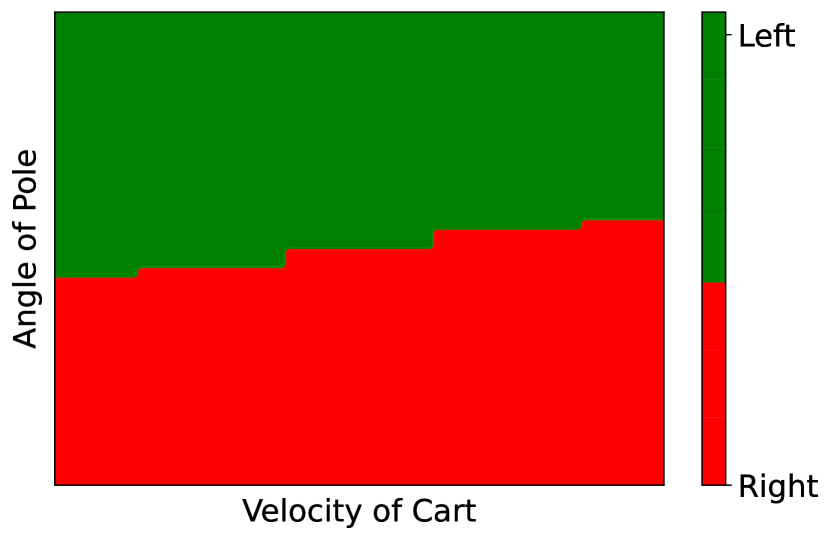
($b$) Decision boundary for the decision-tree approximation

($c$) A four-level decision tree approximating the linear rule

Figure 5. EVOTER versus decision tree representing the linear rule $(0.11*\textit{velocity.of.cart}<0.87*\textit{angle.of.pole})$. ($a$) The decision boundary of the original rule; ($b$) the decision boundary of the ($c$) four-level decision tree approximating it. The color shades in the decision boxes represent different levels of certainty in the decision-making process. Legacy systems represented by the decision tree are less transparent than the explanation discovered by EVOTER through its feature comparison extension.

Second, consider the actual nonlinear rule in Figure 4. The decision boundary is now nonlinear, as seen in Figure 6$a$, and the four-level deep decision tree is an even weaker approximation of it.

Since many physical systems are nonlinear, the ability to represent exponents is crucial in uncovering such relationships. For instance, consider Kepler’s Third Law stating that the squares of the orbital periods of planets are directly proportional to the cubes of the semi-major axes of their orbits. Like many similar laws of nature, this law was initially discovered as an underlying principle of numerous observations. Yet linear models such as decision trees cannot learn it: It is a power law that requires the representation of exponents. This level of complexity exceeds the capabilities of legacy transparent systems like decision trees, highlighting the importance of the nonlinear extension in EVOTER in developing insights in scientific domains.

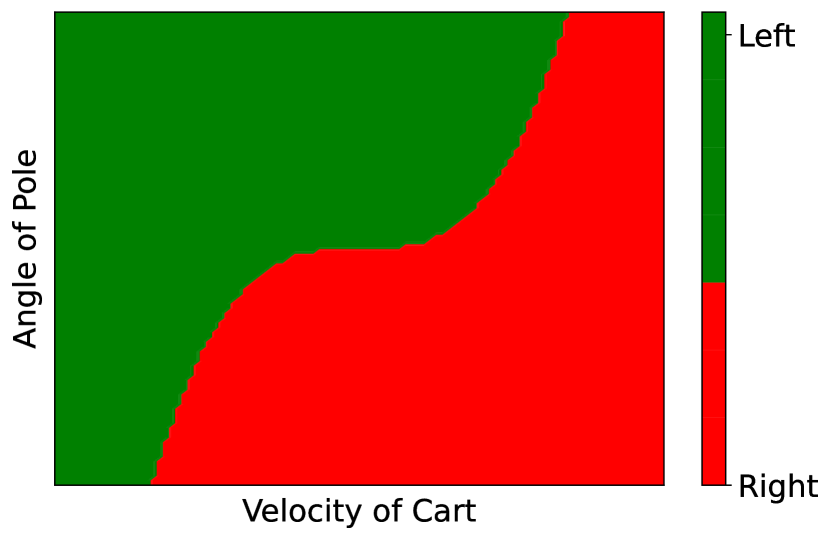
($a$) Decision boundary for the non-linear rule

$$(0.11*{\textit{velocity.of.cart}}^{3}<0.87*\textit{angle.of.pole}) \longrightarrow\hbox{\pagecolor{plotgreen}{\color[rgb]{1,1,1}}}$$

else $$\longrightarrow\hbox{\pagecolor{plotred}{\color[rgb]{1,1,1}}}$$

($b$) Decision boundary for the decision-tree approximation

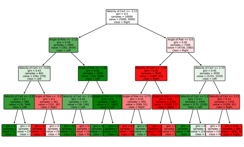
($c$) A four-level decision tree approximating the nonlinear rule

Figure 6. EVOTER versus a decision tree representing the nonlinear rule $(0.11*\textit{velocity.of.cart}^{3}<0.87*\textit{angle.of.pole})$. ($a$) The decision boundary of the original rule; ($b$) the decision boundary of the ($c$) four-level decision tree approximating it, with color shades representing certainty. EVOTER’s nonlinear extension to the rule representation not only offers simplicity and ease of understanding but also maintains precision and accuracy.

4.3. Evolving rule sets with a surrogate (ESP)

Many real-world domains are too costly for direct evolution, and the evaluation of candidates needs to be done more economically against a surrogate model (esp-rl). The next experiment demonstrates that solutions evolved with a surrogate can be remarkably similar to those evolved directly in the domain.

Experiment

Evolutionary Surrogate-Assisted Prescription, or ESP (esp-rl) is a general approach to decision making where the decision policy is discovered through evolution and the surrogate is constructed through machine learning. The surrogate, or the predictor, can be an opaque model such as a random forest or neural network trained with gradient descent. Similarly, the decision policy, or the prescriptor, is often a neural network; however, evolving a rule set to represent the strategy results in an explainable solution instead.

In this experiment, ESP was set up to solve the same cart-pole domain as in the previous section. The prescriptor population was initially random and therefore generated a diverse set of actions. The predictor was trained with the outcome of these actions. The trained predictor was then used to evaluate prescriptor candidates through evolution.

$$1. (0.16*{\textit{velocity.of.cart}}^{3}>0.89*\textit{angle.of.pole}) \longrightarrow\hbox{\pagecolor{plotred}{\color[rgb]{1,1,1}}}$$

$$2. \longrightarrow\hbox{\pagecolor{plotgreen}{\color[rgb]{1,1,1}}}$$ Default Action

Figure 7. A sample rule set discovered through ESP in the Cart-Pole domain. These rules are logically almost identical to those discovered through direct evolution (i.e., Figure 4). This result verifies that a surrogate-based optimization is a viable approach, i.e. it discovers the same solutions as direct evolution.

Results

The predictor trained reliably with 100 action examples from the random initial population. Evolution then took only three generations to find agents that solved the examples in the validation set. Interestingly, the resulting rules (Figure 7) are logically almost identical to those resulting from direct evolution (Figure 4). While this validity of the surrogate modeling approach has been demonstrated before in terms of performance (esp-rl), rule-set evolution makes this conclusion explicit.

4.4. Obtaining insights and avoiding biases

In this experiment, rule-based ESP was applied to the task of recommending medication for hospitalized diabetes patients that would both minimize hospital readmissions and lead to good discharge outcomes. The results were evaluated together with physicians, giving them a plain-text interpretation and indicating insights that are possible to obtain with this approach.

Experiment

The Diabetes data set (diabetes) represents ten years (1999-2008) of clinical care at 130 US hospitals and integrated delivery networks. Information was extracted from the database for encounters that satisfied the following criteria:

• It is an inpatient encounter (a hospital admission).

• It is a diabetic encounter, i.e., one with any kind of diabetes was entered into the system as a diagnosis.

• The length of stay was at least one day and at most 14 days.

• Laboratory tests were performed during the encounter.

• Medications were administered during the encounter.

The data set includes over 50 features characterizing the patient and the hospital context, including patient number, race, gender, age, admission type, time in hospital, the medical specialty of admitting physician, number of lab tests performed, HbA1c test results, and diagnosis, as well as the number of outpatients, inpatients, and emergency visits by the patient in the year before the hospitalization. As actions, 21 different treatments can be prescribed, i.e.,  different diabetic and other medications. Two objectives are optimized: readmission rate and discharge disposition. The three possible readmission categories are: ”no readmission” (+1 point), ”readmission in less than 30 days” (0), and ”readmission in more than 30 days” (-1). The discharge-disposition categories were: ”sent back home” (+2 points), ”remained in the hospital” (-1), ”left with advised medical attention” (-1), ”sent to another hospital” (-1), and ”died” (-4). The goal is to maximize the readmission and discharge-disposition scores simultaneously.

A neural-network predictor was trained with $\sim$66k samples in the historical data, with $\sim$33k reserved for validation and $\sim$33k for testing. A population of 100 rule sets was then evolved for 40 generations to generate a Pareto front: Given the patient and hospital contexts, they represent different tradeoffs between reducing readmissions and improving discharge dispositions. Note that these objectives are somewhat at odds: e.g.,  sending the patient home too early may result in early readmission.

$$1. (\textit{diag1.injury}\leq 2.2*\textit{diag1.respiratory})\And$$

$$(\textit{diag2.neoplasms}>33) \longrightarrow\textit{Metformin-Pioglitazone}$$

$$2. (\textit{age}[60-70)\geq 1.2*\textit{age}[10-20)) \longrightarrow\textit{Glyburide}$$

$$3. (\textit{diag2.diabetes}\geq 0.82*\textit{diag1.digestive}) \longrightarrow\textit{Glipizide- Metformin}$$

$$4. (\textit{admission.Court/Law}\geq 1.045*\textit{diag3.circulatory}) \longrightarrow\textit{Pioglitazone}$$

$$5. (\textit{age}[80-90)\geq 2.29*\textit{admission.type.id.Newborn}) \longrightarrow\textit{Tolazamide}$$

$$6. (\textit{age}[30-40)\leq 0.47*\textit{age}[50-60))\And$$

$$(\textit{admission.type.id.Newborn}\leq 0.47*\textit{age}[50-60))\And$$

$$(\textit{diag2.respiratory}\geq 1.86*\textit{diag3.musculoskeletal})\And$$

$$(\textit{diag1.diabetes}\geq 1.42*\textit{age}[30-40))\And$$

$$(0.18*\textit{gender}\geq 0.38*\textit{race.Asian})\And$$

$$(0.12*\textit{race.AfricanAmerican}\geq 0.15*\textit{admission.Court/Law})\And$$

$$(0.03*\textit{race.Hispanic}\leq 0.76*\textit{admission.Emergency.Room}) \longrightarrow\textit{Insulin}$$

$$7. \longrightarrow\textit{Glipizide}$$ Default

Figure 8. A sample rule set discovered through ESP to reduce hospital readmissions and improve discharge disposition for diabetes. The rules are transparent but contain redundancies that make them sometimes hard to read. A domain expert can verify that the set is meaningful and translate them into plain English where the insights and biases are easier to see (Figure 9).

Results

The predictor training achieved a test accuracy of $\sim$80% (of correct classifications into the three categories). Rule set evolution started with a no-readmission rate of $\sim$29%, which improved to $\sim$49% over the 40 generations; a similar improvement was observed along the discharge-disposition objective. Remarkable tradeoffs were discovered that performed much better than the actual prescriptions in the data set. Whereas 78% of patients were sent home and the no-readmission rate was 60% in the data set, the most dominant solution recommended treatments that were predicted to result in sending home as well as no readmission 99% of the time.

$$1.$$ If the patient has a respiratory problem

but not a neoplasms problem prescribe Metformin-Pioglitazone

$$2.$$ If the patient is any age except 60 to 70 prescribe Glyburide

$$3.$$ If the patient has Diabetic Diagnostic prescribe Glipizide- Metformin

$$4.$$ If the patient has circulatory diagnosis prescribe Pioglitazone

$$5.$$ If the admission type is Newborn prescribe Tolazamide

$$6. ~{}\text{If the patient's age is between 30 to 60}\And$$

$$~{}\text{the patient has musculoskeletal diagnosis}\And$$

$$~{}\text{is not Asian}\And$$

$$~{}\text{was not sent by court/law}\And$$

was admitted in emergency prescribe Insulin

$$7.$$ If none of the above prescribe Glipizide

Figure 9. Expert interpretation of the diabetes treatment rule set. In particular, Rule 6 is now easier to read. It also makes it possible to identify a potential racial bias; in this case, the bias is medically indicated, but in other applications, it may be due to inaccurate training data. Such biases can be identified and edited out when using rule sets, which would be difficult to do with other machine-learning approaches.

Figure 8 shows this highly effective rule set discovered by EVOTER. The rules are relatively transparent but again contain redundancies that make them somewhat difficult to read. To clarify and evaluate them, these rules were given to a domain expert who removed the redundancies and translated them into plain text (Figure 9). For instance, given that their features take on binary values, the last three clauses of Rule 6 can be simplified to ”not Asian”, ”not court/law”, and emergency. The expert verified that, indeed, this set constitutes a meaningful treatment policy.

This example also illustrates the potential of the rule set evolution to make biases in machine learning systems explicit. For instance, rule 6 is conditioned upon the race of the patients being Asian. In this case, race is indeed a medically valid consideration, but it is easy to see that in other domains with incomplete data, such constraints could be simply due to biases in the data. With rule sets, it is possible to identify such biases. Furthermore, it is possible to edit them out when they are not warranted, which would be very difficult to do with other machine-learning approaches.

4.5. Performance of evolved rule-set vs. neural network prescriptors

The standard approach in ESP is to evolve neural networks as the prescriptor. While neural networks are powerful and flexible, they are opaque. On the other hand, rule sets are transparent and interpretable. An essential question is whether rule sets can achieve performance comparable to neural networks in this role. In this section, this question is answered in two different tasks, one (heart-failure prevention) involving a single objective and the other (diabetes treatment) two objectives. In both cases, the performance of rule sets is found only slightly short of that of the neural networks, demonstrating that explainability can be achieved with a minimal cost.

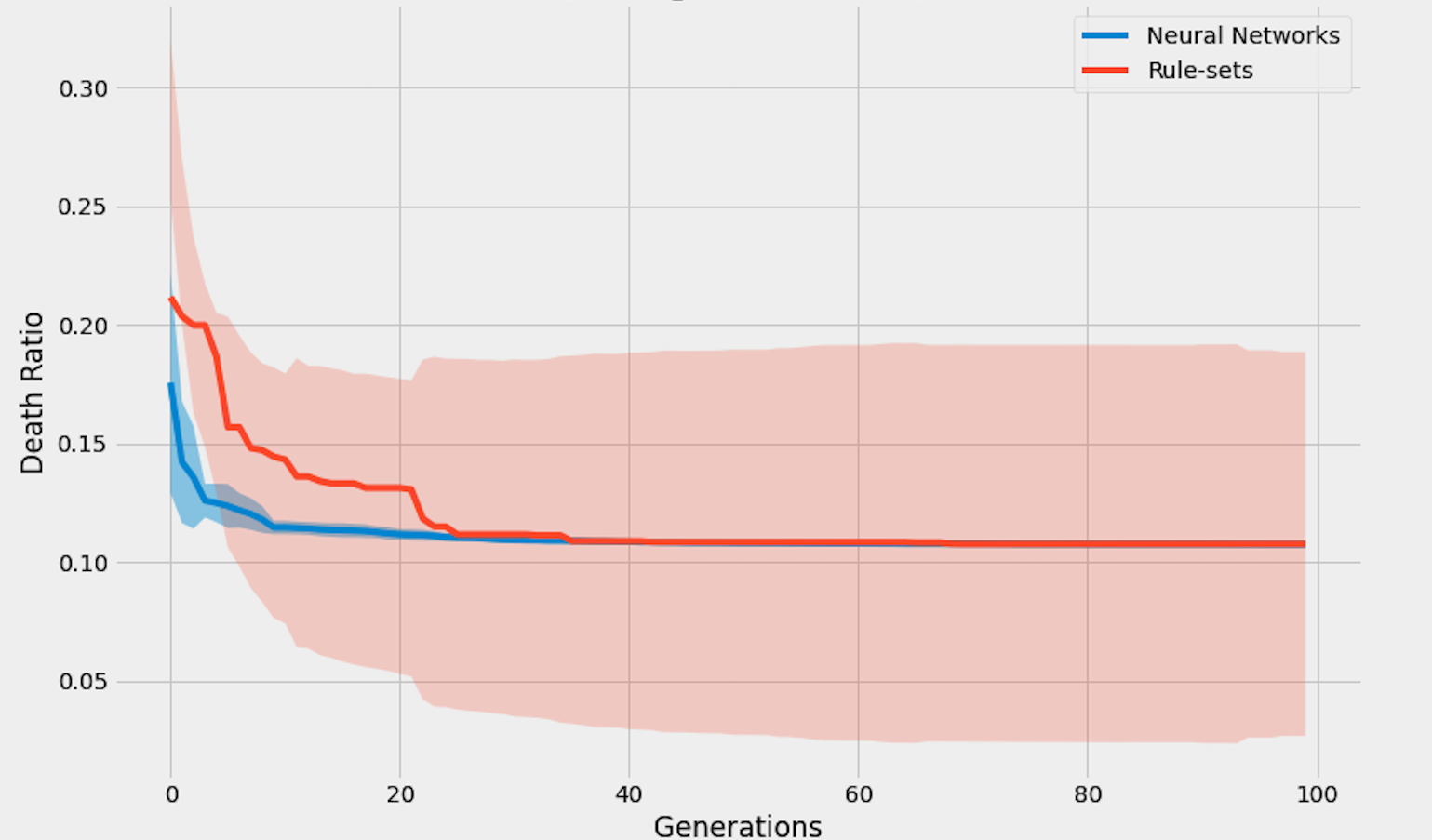
Figure 10. Evolution of neural-network and rule-set prescriptors in the single-objective domain of Heart-Failure Prevention. The plots are averaged over 10 runs and shading indicates 95% confidence intervals. The rule set population varies more throughout evolution, but the final best solutions perform almost the same on average, with a death rate of slightly less than 0.11. The differences are not statistically significant ($p=0.76$). Thus, explainability is achieved with more diversity and practically no cost in performance.

4.5.1. Heart-Failure Prevention recommendation (single objective)

Experiment

A random-forest predictor was trained on the Heart-Failure data set (chicco2020machine) to predict the probability of death for a patient given two possible interventions, i.e., ejection fraction and serum creatinine. The predictor achieved an out-of-sample Mathews correlation coefficient of 0.33.

The prescriptor receives the patient’s condition as its input and prescribes one of the two interventions. The predictor is queried to evaluate its fitness in minimizing deaths. The neural network prescriptor’s input nodes correspond to the patient’s condition and output nodes to the two possible treatments; it has a hidden layer of 16 nodes. Its weights were evolved over 100 generations using a population size of 100. Similarly, the rule-set prescriptor includes left-hand side clauses referring to the patient’s condition and right-hand side actions specifying interventions. Evolution was similarly set to run for 100 generations with a population of 100.

$$1. (0.08*\textit{anaemia}<0.44*\textit{platelets}) \longrightarrow 0.21*\textit{ejection.fraction}$$

$$2. (0.08*\textit{platelets}\leq 0.45[0.0..1.0]) \longrightarrow 0.59*\textit{ejection.fraction}$$

$$3. (0.84*\textit{anaemia}^{3}\leq 0.40*\textit{age}) \longrightarrow 0.04*\textit{serum.creatinine}$$

$$4. (0.89*\textit{serum.sodium}>0.97*\textit{smoking})\And$$

$$(0.47*\textit{serum.sodium}>0.09*\textit{creatinine.phosphokinase}) \longrightarrow 0.32*\textit{ejection.fraction}$$

$$5. (1.00*\textit{age}>0.97*\textit{platelets}) \longrightarrow 0.49*\textit{ejection.fraction}$$

$$6. (0.39*\textit{creatinine.phosphokinase}<0.92*\textit{anaemia}) \longrightarrow 0.03*\textit{serum.creatinine}$$

$$7. (0.94*\textit{platelets}\geq 0.02*\textit{anaemia}) \longrightarrow 0.65*\textit{ejection.fraction}$$

$$8. (0.46*\textit{smoking}\leq 0.50*\textit{diabetes}) \longrightarrow 0.51*\textit{ejection.fraction}$$

$$9. (0.49*\textit{anaemia}\leq 0.92[0.0..1.0])\And$$

$$(0.46*\textit{smoking}\leq 0.50*\textit{diabetes})\And$$

$$(0.09*\textit{platelets}\leq 0.78[0.0..1.0]) \longrightarrow 0.36*\textit{ejection.fraction}$$

$$10. (0.08*\textit{high.blood.pressure}^{3}\leq 0.85*\textit{diabetes}) \longrightarrow 0.21*\textit{ejection.fraction}$$

$$11. (0.91*\textit{platelets}<0.62*\textit{high.blood.pressure})\And$$

$$(0.61*\textit{age}<0.88*\textit{high.blood.pressure})\And$$

$$(0.10*\textit{creatinine.phosphokinase}<0.43*\textit{sex}) \longrightarrow 0.46*\textit{ejection.fraction}$$

$$12. (0.47*\textit{serum.sodium}>0.09*\textit{creatinine.phosphokinase}) \longrightarrow 0.32*\textit{ejection.fraction}$$

$$13. (0.46*\textit{smoking}\leq 0.50*\textit{diabetes})\And$$

$$(0.06*\textit{anaemia}>0.82*\textit{creatinine.phosphokinase})\And$$

$$(0.03*\textit{high.blood.pressure}\geq 0.21*\textit{sex}) \longrightarrow 0.51*\textit{ejection.fraction}$$

$$14. (0.31*\textit{creatinine.phosphokinase}>=0.02*\textit{high.blood.pressure}) \longrightarrow 0.48*\textit{ejection.fraction}$$

$$15. (0.47*\textit{serum.sodium}>0.09*\textit{creatinine.phosphokinase})\And$$

$$(0.40*\textit{diabetes}\geq 0.33*\textit{serum.sodium}) \longrightarrow 0.32*\textit{ejection.fraction}$$

$$16. (0.17*\textit{smoking}<0.30*\textit{high.blood.pressure})\And$$

$$(0.08*\textit{high.blood.pressure}\leq 0.85*\textit{diabetes}) \longrightarrow 0.21*\textit{ejection.fraction}$$

$$17. (0.94*\textit{platelets}\geq 0.02*\textit{anaemia})\And$$

$$(0.46*\textit{smoking}\leq 0.50*\textit{diabetes}) \longrightarrow 0.65*\textit{ejection.fraction}$$

$$18. (1.00*\textit{age}>0.97*\textit{platelets})\And$$

$$(0.97*\textit{platelets}\leq 0.36*\textit{diabetes})\And$$

$$(0.46*\textit{smoking}\leq 0.50*\textit{diabetes}) \longrightarrow 0.49*\textit{ejection.fraction}$$

$$19. (0.46*\textit{smoking}\leq 0.50*\textit{diabetes})\And$$

$$(0.08*\textit{age}>0.85*\textit{diabetes})\And$$

$$(0.03*\textit{high.blood.pressure}\geq 0.21*\textit{sex}) \longrightarrow 0.51*\textit{ejection.fraction}$$

$$20. (0.91*\textit{platelets}<0.62*\textit{high.blood.pressure})\And$$

$$(0.10*\textit{creatinine.phosphokinase}<0.43*\textit{sex}) \longrightarrow 0.46*\textit{ejection.fraction}$$

$$21. (0.46*\textit{smoking}\leq 0.50*\textit{diabetes})\And$$

$$(0.06*\textit{anaemia}>0.82*\textit{creatinine.phosphokinase}) \longrightarrow 0.51*\textit{ejection.fraction}$$

$$22. (0.88*\textit{anaemia}>0.76[0.0..1.0])\And$$

$$(0.84*\textit{creatinine.phosphokinase}<0.40*\textit{age})\And$$

$$(0.45*\textit{sex}<0.85[0.0..1.0]) \longrightarrow 0.04*\textit{serum.creatinine}$$

$$23. (0.46*\textit{smoking}\leq 0.50*\textit{diabetes})\And$$

$$(0.08*\textit{anaemia}<0.44*\textit{platelets}) \longrightarrow 0.21*\textit{ejection.fraction}$$

$$24. (0.63*\textit{high.blood.pressure}\leq 0.79*\textit{serum.sodium})\And$$

$$(0.46*\textit{smoking}\leq 0.50*\textit{diabetes})\And$$

$$(0.31*\textit{creatinine.phosphokinase}\geq 0.02*\textit{high.blood.pressure}) \longrightarrow 0.48*\textit{ejection.fraction}$$

$$25. (0.08*\textit{age}>0.85*\textit{diabetes}) \longrightarrow 0.21*\textit{ejection.fraction}$$

$$26. (0.09*\textit{platelets}\leq 0.78[0.0..1.0])\And$$

$$(0.08*\textit{age}>0.85*\textit{diabetes}) \longrightarrow 0.36*\textit{ejection.fraction}$$

$$27. (0.91*\textit{platelets}<0.62*\textit{high.blood.pressure})\And$$

$$(0.24*\textit{serum.sodium}>0.29*\textit{diabetes})\And$$

$$(0.10*\textit{creatinine.phosphokinase}<0.43*\textit{sex})\And$$

$$(0.08*\textit{age}>0.85*\textit{diabetes}) \longrightarrow 0.46*\textit{ejection.fraction}$$

$$28. (0.91*\textit{platelets}<0.62*\textit{high.blood.pressure}) \longrightarrow 0.46*\textit{ejection.fraction}$$

$$29. (0.40*\textit{diabetes}\geq 0.33*\textit{serum.sodium}) \longrightarrow 0.32*\textit{ejection.fraction}$$

$$30. (0.31*\textit{creatinine.phosphokinase}\geq 0.02*\textit{high.blood.pressure}) \longrightarrow 0.48*\textit{ejection.fraction}$$

$$31. (0.84*\textit{creatinine.phosphokinase}\geq 0.40*\textit{age}) \longrightarrow 0.04*\textit{serum.creatinine}$$

$$32. (0.94*\textit{platelets}\geq 0.02*\textit{anaemia})\And$$

$$(0.08*\textit{platelets}\leq 0.45[0.0..1.0]) \longrightarrow 0.59*\textit{ejection.fraction}$$

$$33. (0.08*\textit{anaemia}<0.44*\textit{platelets})\And$$

$$(0.08*\textit{age}>0.85*\textit{diabetes}) \longrightarrow 0.21*\textit{ejection.fraction}$$

$$34. (0.47*\textit{serum.sodium}>0.09*\textit{creatinine.phosphokinase})\And$$

$$(0.46*\textit{smoking}\leq 0.50*\textit{diabetes})\And$$

$$(0.40*\textit{diabetes}\geq 0.33*\textit{serum.sodium}) \longrightarrow 0.32*\textit{ejection.fraction}$$

$$35. (0.39*\textit{creatinine.phosphokinase}<0.92*\textit{anaemia})\And$$

$$(0.10*\textit{anaemia}\geq 0.06*\textit{serum.sodium}) \longrightarrow 0.03*\textit{serum.creatinine}$$

$$36. (0.91*\textit{platelets}<0.62*\textit{high.blood.pressure})\And$$

$$(0.46*\textit{smoking}\leq 0.50*\textit{diabetes})\And$$

$$(0.10*\textit{creatinine.phosphokinase}<0.43*\textit{sex}) \longrightarrow 0.46*\textit{ejection.fraction}$$

$$37. (0.46*\textit{smoking}\leq 0.50*\textit{diabetes})\And$$

$$(0.08*\textit{age}\leq 0.85*\textit{diabetes}) \longrightarrow 0.21*\textit{ejection.fraction}$$

$$38. (0.46*\textit{smoking}\leq 0.50*\textit{diabetes})\And$$

$$(0.08*\textit{platelets}\leq 0.45[0.0..1.0]) \longrightarrow 0.59*\textit{ejection.fraction}$$

$$39. (0.46*\textit{smoking}\leq 0.50*\textit{diabetes})\And$$

$$(0.03*\textit{high.blood.pressure}\geq 0.21*\textit{sex}) \longrightarrow 0.51*\textit{ejection.fraction}$$

$$40. (0.41*\textit{high.blood.pressure}>0.48*\textit{sex})\And$$

$$(0.09*\textit{platelets}\leq 0.78[0.0..1.0])\And$$

$$(0.08*\textit{age}>0.85*\textit{diabetes}) \longrightarrow 0.36*\textit{ejection.fraction}$$

$$41. (0.46*\textit{smoking}\leq 0.50*\textit{diabetes})\And$$

$$(0.09*\textit{platelets}\leq 0.78[0.0..1.0]) \longrightarrow 0.36*\textit{ejection.fraction}$$

$$42. (0.21*\textit{high.blood.pressure}\leq 0.85*\textit{diabetes})\And$$

$$(0.17*\textit{smoking}<0.30*\textit{high.blood.pressure}) \longrightarrow 0.21*\textit{ejection.fraction}$$

$$43. (1.00*\textit{age}>0.97*\textit{platelets})\And$$

$$(0.97*\textit{platelets}\leq 0.36*\textit{diabetes}) \longrightarrow 0.49*\textit{ejection.fraction}$$

$$44. (0.97*\textit{platelets}\leq 0.36*\textit{diabetes}) \longrightarrow 0.49*\textit{ejection.fraction}$$

$$45. (0.23*\textit{diabetes}>0.89*\textit{platelets})\And$$

$$(0.08*\textit{high.blood.pressure}^{3}\leq 0.85*\textit{diabetes}) \longrightarrow 0.21*\textit{ejection.fraction}$$

$$46. (0.14*\textit{creatinine.phosphokinase}>0.75*\textit{smoking})\And$$

$$(0.08*\textit{age}\leq 0.85*\textit{diabetes}) \longrightarrow 0.21*\textit{ejection.fraction}$$

$$47. \longrightarrow 0.13*\textit{serum.creatinine}$$ Default

Figure 11. A sample solution rule set for the Heart-Failure Prevention domain. The default rule indicates serum, and the others mostly identify situations where ejection fraction is preferable. Many of the rules are redundant, which is a common result of the search process. Based on the times_applied counters, those rules can be removed, resulting in a compact set shown in Figure 12.

$$1.\hskip 6.93195pt(1.)\hskip 3.31529pt83 \hskip 3.31529pt(0.08*\textit{anaemia}<0.44*\textit{platelets}) \longrightarrow 0.21*\textit{ejection.fraction}$$

$$2.\hskip 3.31529pt(40.)\hskip 3.31529pt66 \hskip 3.31529pt(0.89*\textit{serum.sodium}>0.97*\textit{smoking})\And$$

$$\hskip 3.31529pt(0.47*\textit{serum.sodium}>0.09*\textit{creatinine.phosphokinase}) \longrightarrow 0.32*\textit{ejection.fraction}$$

$$3.\hskip 6.63052pt(8.)102 \hskip 3.31529pt(0.46*\textit{smoking}\leq 0.50*\textit{diabetes}) \longrightarrow 0.51*\textit{ejection.fraction}$$

$$4.\hskip 3.31529pt(10.)\hskip 3.31529pt78 \hskip 3.31529pt(0.08*\textit{high.blood.pressure}^{3}\leq 0.85*\textit{diabetes}) \longrightarrow 0.21*\textit{ejection.fraction}$$

$$5.\hskip 3.31529pt(11.)\hskip 6.63052pt6 \hskip 3.31529pt(0.91*\textit{platelets}<0.62*\textit{high.blood.pressure})\And$$

$$\hskip 3.31529pt(0.61*\textit{age}<0.88*\textit{high.blood.pressure})\And$$

$$\hskip 3.31529pt(0.10*\textit{creatinine.phosphokinase}<0.43*\textit{sex}) \longrightarrow 0.46*\textit{ejection.fraction}$$

$$6.\hskip 3.31529pt(12.)\hskip 3.31529pt73 \hskip 3.31529pt(0.47*\textit{serum.sodium}>0.09*\textit{creatinine.phosphokinase}) \longrightarrow 0.32*\textit{ejection.fraction}$$

$$7.\hskip 3.31529pt(13.)\hskip 3.31529pt11 \hskip 3.31529pt(0.46*\textit{smoking}\leq 0.50*\textit{diabetes})\And$$

$$\hskip 3.31529pt(0.06*\textit{anaemia}>0.82*\textit{creatinine.phosphokinase})\And$$

$$\hskip 3.31529pt(0.03*\textit{high.blood.pressure}\geq 0.21*\textit{sex}) \longrightarrow 0.51*\textit{ejection.fraction}$$

$$8.\hskip 3.31529pt(14.)108 \hskip 3.31529pt(0.31*\textit{creatinine.phosphokinase}>=0.02*\textit{high.blood.pressure}) \longrightarrow 0.48*\textit{ejection.fraction}$$

$$9.\hskip 3.31529pt(15.)\hskip 3.31529pt37 \hskip 3.31529pt(0.47*\textit{serum.sodium}>0.09*\textit{creatinine.phosphokinase})\And$$

$$\hskip 3.31529pt(0.40*\textit{diabetes}\geq 0.33*\textit{serum.sodium}) \longrightarrow 0.32*\textit{ejection.fraction}$$

$$10.\hskip 3.31529pt(16.)\hskip 3.31529pt31 \hskip 3.31529pt(0.17*\textit{smoking}<0.30*\textit{high.blood.pressure})\And$$

$$\hskip 3.31529pt(0.08*\textit{high.blood.pressure}\leq 0.85*\textit{diabetes}) \longrightarrow 0.21*\textit{ejection.fraction}$$

$$11.\hskip 3.31529pt(19.)\hskip 6.63052pt8 \hskip 3.31529pt(0.46*\textit{smoking}\leq 0.50*\textit{diabetes})\And$$

$$\hskip 3.31529pt(0.08*\textit{age}>0.85*\textit{diabetes})\And$$

$$\hskip 3.31529pt(0.03*\textit{high.blood.pressure}\geq 0.21*\textit{sex}) \longrightarrow 0.51*\textit{ejection.fraction}$$

$$12.\hskip 3.31529pt(20.)\hskip 3.31529pt26 \hskip 3.31529pt(0.91*\textit{platelets}<0.62*\textit{high.blood.pressure})\And$$

$$\hskip 3.31529pt(0.10*\textit{creatinine.phosphokinase}<0.43*\textit{sex}) \longrightarrow 0.46*\textit{ejection.fraction}$$

$$13.\hskip 3.31529pt(23.)\hskip 3.31529pt14 \hskip 3.31529pt(0.46*\textit{smoking}\leq 0.50*\textit{diabetes})\And$$

$$\hskip 3.31529pt(0.08*\textit{anaemia}<0.44*\textit{platelets}) \longrightarrow 0.21*\textit{ejection.fraction}$$

$$14.\hskip 3.31529pt(28.)\hskip 3.31529pt73 \hskip 3.31529pt(0.91*\textit{platelets}<0.62*\textit{high.blood.pressure}) \longrightarrow 0.46*\textit{ejection.fraction}$$

$$15.\hskip 3.31529pt(30.)103 \hskip 3.31529pt(0.31*\textit{creatinine.phosphokinase}\geq 0.02*\textit{high.blood.pressure}) \longrightarrow 0.48*\textit{ejection.fraction}$$

$$16.\hskip 3.31529pt(31.)\hskip 3.31529pt97 \hskip 3.31529pt(0.84*\textit{creatinine.phosphokinase}\geq 0.40*\textit{age}) \longrightarrow 0.04*\textit{serum.creatinine}$$

$$17.\hskip 3.31529pt(33.)\hskip 3.31529pt18 \hskip 3.31529pt(0.08*\textit{anaemia}<0.44*\textit{platelets})\And$$

$$\hskip 3.31529pt(0.08*\textit{age}>0.85*\textit{diabetes}) \longrightarrow 0.21*\textit{ejection.fraction}$$

$$18.\hskip 3.31529pt(35.)\hskip 3.31529pt21 \hskip 3.31529pt(0.39*\textit{creatinine.phosphokinase}<0.92*\textit{anaemia})\And$$

$$\hskip 3.31529pt(0.10*\textit{anaemia}\geq 0.06*\textit{serum.sodium}) \longrightarrow 0.03*\textit{serum.creatinine}$$

$$19.\hskip 3.31529pt(36.)\hskip 6.63052pt6 \hskip 3.31529pt(0.91*\textit{platelets}<0.62*\textit{high.blood.pressure})\And$$

$$\hskip 3.31529pt(0.46*\textit{smoking}\leq 0.50*\textit{diabetes})\And$$

$$\hskip 3.31529pt(0.10*\textit{creatinine.phosphokinase}<0.43*\textit{sex}) \longrightarrow 0.46*\textit{ejection.fraction}$$

$$20.\hskip 3.31529pt(37.)\hskip 3.31529pt14 \hskip 3.31529pt(0.46*\textit{smoking}\leq 0.50*\textit{diabetes})\And$$

$$\hskip 3.31529pt(0.08*\textit{age}\leq 0.85*\textit{diabetes}) \longrightarrow 0.21*\textit{ejection.fraction}$$

$$21.\hskip 3.31529pt(38.)\hskip 3.31529pt32 \hskip 3.31529pt(0.46*\textit{smoking}\leq 0.50*\textit{diabetes})\And$$

$$\hskip 3.31529pt(0.08*\textit{platelets}\leq 0.45[0.0..1.0]) \longrightarrow 0.59*\textit{ejection.fraction}$$

$$22.\hskip 3.31529pt(39.)\hskip 3.31529pt15 \hskip 3.31529pt(0.46*\textit{smoking}\leq 0.50*\textit{diabetes})\And$$

$$\hskip 3.31529pt(0.03*\textit{high.blood.pressure}\geq 0.21*\textit{sex}) \longrightarrow 0.51*\textit{ejection.fraction}$$

$$23.\hskip 3.31529pt(40.)\hskip 6.63052pt9 \hskip 3.31529pt(0.41*\textit{high.blood.pressure}>0.48*\textit{sex})\And$$

$$\hskip 3.31529pt(0.09*\textit{platelets}\leq 0.78[0.0..1.0])\And$$

$$\hskip 3.31529pt(0.08*\textit{age}>0.85*\textit{diabetes}) \longrightarrow 0.36*\textit{ejection.fraction}$$

$$24.\hskip 3.31529pt(41.)\hskip 3.31529pt17 \hskip 3.31529pt(0.46*\textit{smoking}\leq 0.50*\textit{diabetes})\And$$

$$\hskip 3.31529pt(0.09*\textit{platelets}\leq 0.78[0.0..1.0]) \longrightarrow 0.36*\textit{ejection.fraction}$$

$$25.\hskip 3.31529pt(42.)\hskip 3.31529pt32 \hskip 3.31529pt(0.21*\textit{high.blood.pressure}\leq 0.85*\textit{diabetes})\And$$

$$\hskip 3.31529pt(0.17*\textit{smoking}<0.30*\textit{high.blood.pressure}) \longrightarrow 0.21*\textit{ejection.fraction}$$

$$26.\hskip 3.31529pt(43.)\hskip 3.31529pt15 \hskip 3.31529pt(1.00*\textit{age}>0.97*\textit{platelets})\And$$

$$\hskip 3.31529pt(0.97*\textit{platelets}\leq 0.36*\textit{diabetes}) \longrightarrow 0.49*\textit{ejection.fraction}$$

$$27.\hskip 3.31529pt(44.)\hskip 3.31529pt72 \hskip 3.31529pt(0.97*\textit{platelets}\leq 0.36*\textit{diabetes}) \longrightarrow 0.49*\textit{ejection.fraction}$$

$$28.\hskip 3.31529pt(45.)\hskip 3.31529pt23 \hskip 3.31529pt(0.23*\textit{diabetes}>0.89*\textit{platelets})\And$$

$$\hskip 3.31529pt(0.08*\textit{high.blood.pressure}^{3}\leq 0.85*\textit{diabetes}) \longrightarrow 0.21*\textit{ejection.fraction}$$

$$29.\hskip 3.31529pt(47.)\hskip 3.31529pt10 \longrightarrow 0.13*\textit{serum.creatinine}$$ Default

Figure 12. Solution rule set from Figure 11 compressed by pruning inactive rules. The original rule number is in parenthesis, followed by the number of times the rule was applied (out of 300 samples). This set is functionally equivalent but much smaller. Also, on average only four rules are active for each case in the dataset. Such conciseness makes interpretation and explanation easier, supporting applications in safety-critical fields such as healthcare, finance, and law.

Results

Effectiveness of the two prescriptor models in preventing death is shown over evolution time in Figure 10, averaged over ten runs. It took more generations for rule set evolution to reach the same level as the neural network evolution, and there is more diversity and variance in the rule set populations. The likely reason is that even small changes in rules (e.g., adding or removing a clause) can have a large effect on performance. However, on average, the final results are very similar: The best rule set performs at 10.8% and the best neural network at 10.7%. Thus, explainability is achieved with practically no cost in performance. With such variability, an interesting question is: How can one candidate be chosen in the end such that it most likely generalizes to unseen data, given the multiple hypothesis problem (avdeeva_1966; mht2014)? It turns out that under a smoothness assumption that similar candidates perform similarly, picking a candidate based on the average performance of its neighbors provides a viable strategy (miikkulainen:ssci17).

A sample rule-set solution is shown in Figure 11. This rule set prioritizes scenarios where the ejection fraction is favorable and utilizes serum creatinine as the default prescription. As discussed in Section 4.2.1, there are many redundant rules as well. To improve interpretability, rules with times_applied=0 were pruned, resulting in a much smaller set with 29, as shown in Figure 12. Each of these rules participates in making decisions on this dataset, however, only four of them are activated for a given input on average. Such conciseness makes interpretation and explanation easier: It is possible to gain a clear understanding of the key factors driving the decision-making process in the domain. Such transparency and interpretability makes it possible to deploy AI systems in safety-critical fields such as healthcare, finance, and law.

4.5.2. Diabetes Treatment recommendation (multiobjective)

($a$) Readmission likelihood

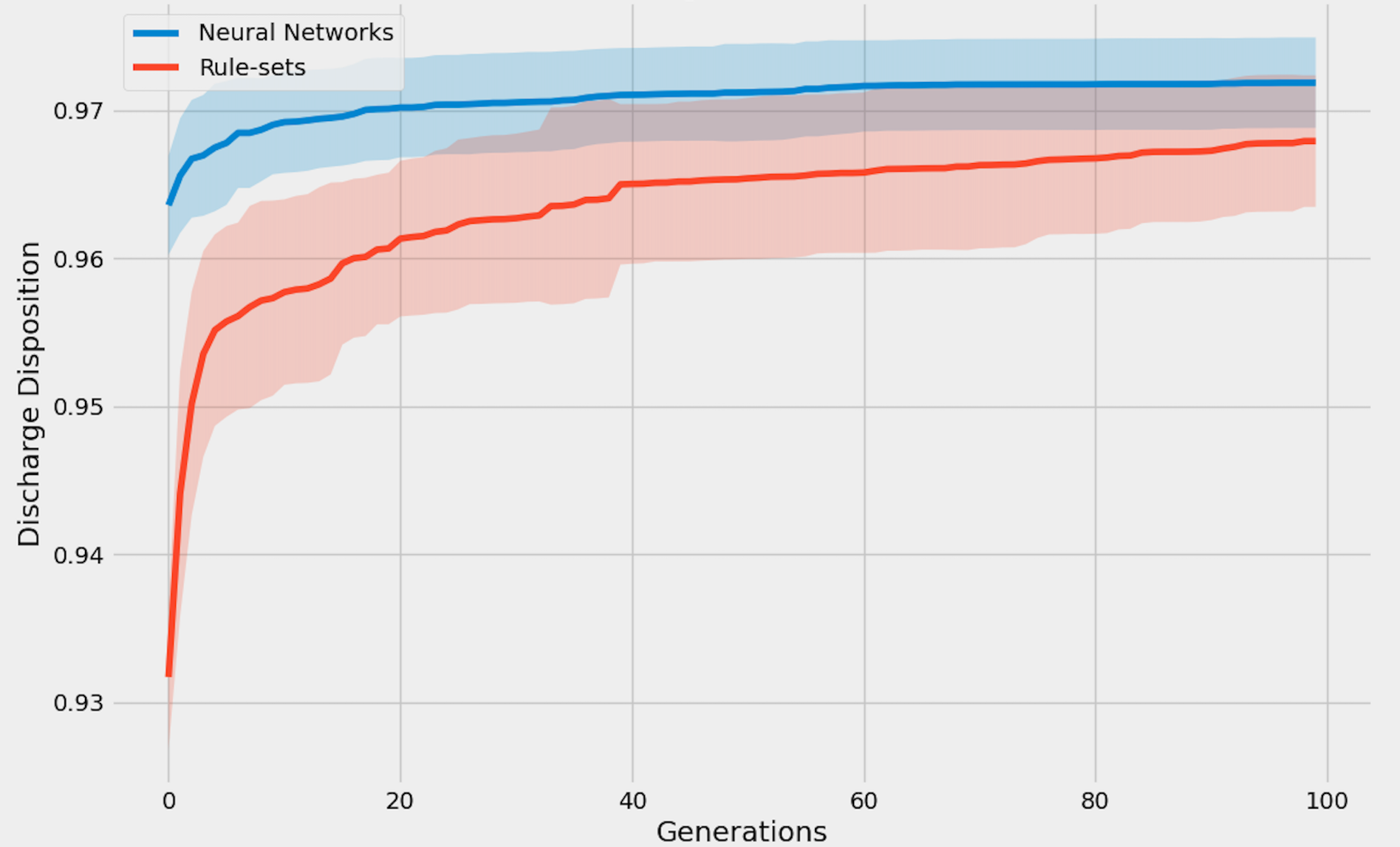
($b$) Discharge disposition quality

Figure 13. Evolution of neural-network and rule-set prescriptors in the multiobjective domain of Diabetes Treatment. ($a$) Progress in the readmission objective and ($b$) discharge disposition objective over evolution; the graphs are averages over 10 runs and shaded areas indicate 95% confidence intervals. While the rule-set population exhibits more variation during evolution, the overlapping confidence intervals suggest that the performance differences between the two approaches are small ($p=0.0012$ in $a$ and $p=0.0327$ in $b$), thus justifying the cost of explainability.

Experiment

In order to assess the cost of explainability in a domain with multiple objectives, a second comparison was run on the same Diabetes Treatment recommendation task as in Section 4.4. Again, the goal was to minimize hospital readmissions while simultaneously improving discharge dispositions. Rule-based ESP was again used to evolve a population of 100 rule sets and 100 neural networks over 100 generations, and evolution repeated ten times..

Results

Figure 13 provides an overview of the results obtained. Again, the variation in the evolved rule sets is slightly higher compared to the neural networks across the ten runs. This variation can be attributed to the discrete nature of the rule set components in contrast to the continuous values of the weights in neural networks. Although the average performance curves are noticeably different, their confidence intervals still overlap. This result suggests that the performance cost associated with the explainability provided by the rule sets is small (i.e. barely significant).

In sum, the experiments in both the single and the multiobjective domain suggest that there may be a small cost in performance when evolving rule sets vs. neural network prescriptors. Depeonding on the domain, such cost may be well worth it in order to achieve transparent, explainable performance.

5. Discussion and Future Work

The experiments presented in this paper suggest that rule-set evolution in general and its EVOTER implementation in particular is a practical and effective approach to machine-learning. EVOTER applies to a wide range of tasks, including prediction, classification, prescription, and policy search, both in static and time-series contexts. It is possible to discover solutions directly in the domain, or through surrogate models that represent the domain in a safe and cost-effective manner. Most importantly, compared to black-box models such as neural networks, rule-set solutions are transparent and explainable. They can provide insight into the domain, uncovering fundamental principles as well as hidden biases. While there may be a slight performance cost compared to black-box models, it may be well worth it in many safety-critical domains.

There are several compelling directions for future work. First, while the time-lag extensions has already proven useful in several time-series domains, its variants can be evaluated further to find the most effective implementations. A fundamental experiment would compare a single variable with a lag parameter, such as ”variable[lag]”, with multiple independent variables that each stand for the different lags, such as ”variable_lag_0”, ”variable_lag_1”, ”variable_lag_2”, and so forth. Such an experiment is expected to confirm the hypothesis that searching for the proper variables first and proper lags second provides an advantage in discovering solutions for time-series problems.

An interesting technical extension would be to expand the expression vocabulary during evolution gradually. For example, the process could be started with a restricted set of operators which could then be expanded as evolution progresses, thus implementing a form of curricular learning.

A useful practical extension to EVOTER would be to include a facility for the expert to edit the discovered rule sets. First, such a facility could be used to identify and remove redundancies, making the rules easier to read. Although much of such simplification can be done automatically, there is still room for human insight. Second, the facility can provide a means for removing biases and making sure that the models are fair. Unlike with opaque models, the learned biases are explicit and can be evaluated and edited out if desired. Third, it may be possible to edit the rules to add further knowledge that may be well understood but challenging to learn, such as safety limits and other real-world constraints.

More generally, it may be possible to build rule-set twins for existing SoTA black-box models. In this manner, converting an opaque but well-performing model into a transparent rule-set equivalent may be possible. This model can then be used to explain the learned behavior and identify its biases and potential weaknesses. Such rule-set models are executable, and if they replicate the performance of the black-box model accurately enough, they could be deployed instead of the black box in explanation-critical applications. In this manner, the process of rule set distillation can play a vital role in deploying machine learning systems in the real world.

To encourage adoption further, Large Language Models (LLMs) (anil:arxiv23; bubeck:arxiv23; touvron:arxiv23) could be used to translate EVOTER rules into plain language. Given the propositional rules as input, LLMs should be able to generate natural language explanations, descriptions, and interpretations. This approach would enable users with varying levels of expertise to comprehend the underlying concepts and their function. It could thus potentially bridge the gap between intricate machine learning techniques and broader audience, making it adoption of such systems easier.

6. Conclusion

This study demonstrated rule-set evolution, implemented in EVOTER, as a promising approach to developing inherently transparent and explainable models. The approach contrasts with the dominant black-box models, such as neural networks, in machine learning. Rule-set evolution can be applied to various tasks, including prediction, classification, prescription, and policy search, to both static and time-series problems, and with and without surrogate models of the domain. While a slight performance cost can be expected compared to black-box models, it may be acceptable in many cases considering the benefits of explainability. Rule-set evolution can thus enhance the trust, understanding, and adoption of AI systems in practical applications.

References

- (1)
- Adadi and Berrada (2018) Amina Adadi and Mohammed Berrada. 2018. Peeking Inside the Black-Box: A Survey on Explainable Artificial Intelligence (XAI). IEEE Access 6 (2018), 52138–52160.
- Austin et al. (2014) RS Austin, Isaac Dialsingh, and NS Altman. 2014. Multiple Hypothesis Testing: A Review. Journal of the Indian Society of Agricultural Statistics 68 (01 2014), 303–314.
- Avdeeva (1966) Ligiia Igorevna Avdeeva. 1966. Simultaneous statistical inference. Springer.
- Belle and Papantonis (2021) Vaishak Belle and Ioannis Papantonis. 2021. Principles and Practice of Explainable Machine Learning. Frontiers in Big Data 4 (2021).
- Brockman et al. (2016) Greg Brockman, Vicki Cheung, Ludwig Pettersson, Jonas Schneider, John Schulman, Jie Tang, and Wojciech Zaremba. 2016. OpenAI Gym. arXiv:1606.01540 (2016).
- Bubeck et al. (2023) Sébastien Bubeck, Varun Chandrasekaran, Ronen Eldan, Johannes Gehrke, Eric Horvitz, Ece Kamar, Peter Lee, Yin Tat Lee, Yuanzhi Li, Scott Lundberg, Harsha Nori, Hamid Palangi, Marco Tulio Ribeiro, and Yi Zhang. 2023. Sparks of Artificial General Intelligence: Early experiments with GPT-4. arXiv:2303.12712 (2023).
- Chicco and Jurman (2020) Davide Chicco and Giuseppe Jurman. 2020. Machine learning can predict survival of patients with heart failure from serum creatinine and ejection fraction alone. BMC medical informatics and decision making 20, 1 (2020), 1–16.
- Deb et al. (2002) K. Deb, A. Pratap, S. Agarwal, and T. Meyarivan. 2002. A fast and elitist multiobjective genetic algorithm: NSGA-II. IEEE Transactions on Evolutionary Computation 6, 2 (2002), 182–197. https://doi.org/10.1109/4235.996017
- Doshi-Velez and Kim (2017) Finale Doshi-Velez and Been Kim. 2017. Towards A Rigorous Science of Interpretable Machine Learning. arXiv:1702:08608 (2017).
- Dua and Graff (2017) Dheeru Dua and Casey Graff. 2017. UCI Machine Learning Repository. http://archive.ics.uci.edu/ml
- et al. (2023) Rohan Anil et al. 2023. PaLM 2 Technical Report. arXiv:2305.10403 (2023).
- Francon et al. (2020) Olivier Francon, Santiago Gonzalez, Babak Hodjat, Elliot Meyerson, Risto Miikkulainen, Xin Qiu, and Hormoz Shahrzad. 2020. Effective reinforcement learning through evolutionary surrogate-assisted prescription. In Proceedings of the 2020 Genetic and Evolutionary Computation Conference. 814–822.
- Gomez and Miikkulainen (1997) Faustino Gomez and Risto Miikkulainen. 1997. Incremental evolution of complex general behavior. Adaptive Behavior 5, 3-4 (1997), 317–342.
- Gunning and Aha (2019) David Gunning and David Aha. 2019. DARPA’s Explainable Artificial Intelligence (XAI) Program. AI Magazine 40, 2 (Jun. 2019), 44–58.
- Hemberg et al. (2014) Erik Hemberg, Kalyan Veeramachaneni, Babak Hodjat, Prashan Wanigasekara, Hormoz Shahrzad, and Una-May O’Reilly. 2014. Learning Decision Lists with Lags for Physiological Time Series. In Third Workshop on Data Mining for Medicine and Healthcare, at the 14th SIAM International Conference on Data Mining. 82–87.
- Hodjat and Shahrzad (2013) Babak Hodjat and Hormoz Shahrzad. 2013. Introducing an Age-Varying Fitness Estimation Function. 59–71. https://doi.org/10.1007/978-1-4614-6846-2_5
- Hodjat et al. (2018) Babak Hodjat, Hormoz Shahrzad, Risto Miikkulainen, Lawrence Murray, and Chris Holmes. 2018. PRETSL: Distributed Probabilistic Rule Evolution for Time-Series Classification. In Genetic Programming Theory and Practice XIV. Springer, 139–148.
- Jacques et al. (2015) Julie Jacques, Julien Taillard, David Delerue, Clarisse Dhaenens, and Laetitia Jourdan. 2015. Conception of a dominance-based multi-objective local search in the context of classification rule mining in large and imbalanced data sets. Applied Soft Computing 34 (2015), 705–720.
- Lage et al. (2019) Isaac Lage, Emily Chen, Jeffrey He, Menaka Narayanan, Been Kim, Sam Gershman, and Finale Doshi-Velez. 2019. An evaluation of the human-interpretability of explanation. arXiv:1902.00006 (2019).
- Lakkaraju et al. (2019) Himabindu Lakkaraju, Ece Kamar, Rich Caruana, and Jure Leskovec. 2019. Faithful and Customizable Explanations of Black Box Models. In Proceedings of the 2019 AAAI/ACM Conference on AI, Ethics, and Society (Honolulu, HI, USA) (AIES ’19). Association for Computing Machinery, New York, NY, USA, 131–138.
- Linardatos et al. (2020) Pantelis Linardatos, Vasilis Papastefanopoulos, and Sotiris Kotsiantis. 2020. Explainable ai: A review of machine learning interpretability methods. Entropy 23, 1 (2020), 18.
- Lundberg and Lee (2017) Scott M Lundberg and Su-In Lee. 2017. A unified approach to interpreting model predictions. Advances in neural information processing systems 30 (2017).
- Miikkulainen et al. (2021) Risto Miikkulainen, Olivier Francon, Elliot Meyerson, Xin Qiu, Darren Sargent, Elisa Canzani, and Babak Hodjat. 2021. From Prediction to Prescription: Evolutionary Optimization of Non-Pharmaceutical Interventions in the COVID-19 Pandemic. IEEE Transactions on Evolutionary Computation 25 (2021), 386–401.
- Miikkulainen et al. (2017) Risto Miikkulainen, Hormoz Shahrzad, Nigel Duffy, and Phil Long. 2017. How to Select a Winner in Evolutionary Optimization?. In Proceedings of the IEEE Symposium Series in Computational Intelligence. IEEE. http://www.cs.utexas.edu/users/ai-lab?miikkulainen:ssci17
- Miller (2019) Tim Miller. 2019. Explanation in artificial intelligence: Insights from the social sciences. Artificial intelligence 267 (2019), 1–38.
- Peñarroya (2004) Jaume Bacardit Peñarroya. 2004. Pittsburgh genetic-based machine learning in the data mining era: representations, generalization, and run-time.
- Poghosyan et al. (2021) Arnak Poghosyan, Ashot Harutyunyan, Naira Grigoryan, and Nicholas Kushmerick. 2021. Incident Management for Explainable and Automated Root Cause Analysis in Cloud Data Centers. Journal of Universal Computer Science 27, 11 (2021), 1152–1173.
- Qiu et al. (2020) Xin Qiu, Elliot Meyerson, and Risto Miikkulainen. 2020. Quantifying Point-Prediction Uncertainty in Neural Networks via Residual Estimation with an I/O Kernel. In Proceedings of the International Conference on Learning Representations.
- Ribeiro et al. (2016) Marco Tulio Ribeiro, Sameer Singh, and Carlos Guestrin. 2016. ”Why Should I Trust You?”: Explaining the Predictions of Any Classifier. In Proceedings of the 22nd ACM SIGKDD International Conference on Knowledge Discovery and Data Mining (San Francisco, California, USA) (KDD ’16). Association for Computing Machinery, New York, NY, USA, 1135–1144.
- Schmidt and Lipson (2009) Michael Schmidt and Hod Lipson. 2009. Distilling Free-Form Natural Laws from Experimental Data. Science 324, 5923 (2009), 81–85.
- Shahrzad et al. (2018) Hormoz Shahrzad, Daniel Fink, and Risto Miikkulainen. 2018. Enhanced Optimization with Composite Objectives and Novelty Selection. In Proceedings of the 2018 Conference on Artificial Life. Tokyo, Japan. http://www.cs.utexas.edu/users/ai-lab?shahrzad:alife18
- Shahrzad et al. (2020) Hormoz Shahrzad, Babak Hodjat, Camille Dolle, Andrej Denissov, Simon Lau, Donn Goodhew, Justin Dyer, and Risto Miikkulainen. 2020. Enhanced Optimization with Composite Objectives and Novelty Pulsation. In Genetic Programming Theory and Practice XVII, Wolfgang Banzhaf, Erik Goodman, Leigh Sheneman, Leonardo Trujillo, and Bill Worzel (Eds.). Springer, New York, 275–293.
- Shahrzad et al. (2016) Hormoz Shahrzad, Babak Hodjat, and Risto Miikkulainen. 2016. Estimating the Advantage of Age-Layering in Evolutionary Algorithms. 693–699. https://doi.org/10.1145/2908812.2908911
- Srinivasan and Ramakrishnan (2011) Sujatha Srinivasan and Sivakumar Ramakrishnan. 2011. Evolutionary multi objective optimization for rule mining: A review. Artificial Intelligence Review 36 (10 2011), 205–248. https://doi.org/10.1007/s10462-011-9212-3
- Strack et al. (2014) Beata Strack, Jonathan Deshazo, Chris Gennings, Juan Luis Olmo Ortiz, Sebastian Ventura, Krzysztof Cios, and John Clore. 2014. Impact of HbA1c Measurement on Hospital Readmission Rates: Analysis of 70,000 Clinical Database Patient Records. BioMed Research International 2014 (2014), 781670.
- Tasfi (2016) Norman Tasfi. 2016. PyGame Learning Environment. https://github.com/ntasfi/PyGame-Learning-Environment.
- Tjoa and Guan (2021) Erico Tjoa and Cuntai Guan. 2021. A Survey on Explainable Artificial Intelligence (XAI): Toward Medical XAI. IEEE Transactions on Neural Networks and Learning Systems 32 (2021), 4793–4813.
- Touvron et al. (2023) Hugo Touvron, Thibaut Lavril, Gautier Izacard, Xavier Martinet, Marie-Anne Lachaux, Timothée Lacroix, Baptiste Rozière, Naman Goyal, Eric Hambro, Faisal Azhar, Aurelien Rodriguez, Armand Joulin, Edouard Grave, and Guillaume Lample. 2023. LLaMA: Open and Efficient Foundation Language Models. arXiv:2302.13971 (2023).
- Townsend et al. (2019) Joseph Townsend, Thomas Chaton, and Joao M Monteiro. 2019. Extracting relational explanations from deep neural networks: A survey from a neural-symbolic perspective. IEEE transactions on neural networks and learning systems 31, 9 (2019), 3456–3470.