Lightweight Hybrid CNN-ELM Model for Multi-building and Multi-floor Classification

Abstract

Machine learning models have become an essential tool in current indoor positioning solutions, given their high capabilities to extract meaningful information from the environment. Convolutional neural networks (CNNs) are one of the most used neural networks (NNs) due to that they are capable of learning complex patterns from the input data. Another model used in indoor positioning solutions is the Extreme Learning Machine (ELM), which provides an acceptable generalization performance as well as a fast speed of learning. In this paper, we offer a lightweight combination of CNN and ELM, which provides a quick and accurate classification of building and floor, suitable for power and resource-constrained devices. As a result, the proposed model is $58\%$ faster than the benchmark, with a slight improvement in the classification accuracy (by less than $1\%$).

I Introduction

In the last two decades, the use of Machine Learning (ML) algorithms in indoor positioning solutions are becoming more and more frequent, because of their high performance and accuracy. Thus, industry and academia are developing new ML models to provide highly accurate solutions to the end-users. Some of these ML models are already used in Internet of Things (IoT) and wearable devices [1]. In this case, it is essential to keep a low computational load and high accuracy. There is, however, a trade-off between accuracy and computational complexity. The more accurate a model, the more computational resources used; finding an equilibrium between accuracy and power consumption has become a hot topic in ML [2].

Given the rapid growth of wearable and IoT devices that use positioning and localization services, it is essential to provide models that empower indoor positioning solutions in power-constrained devices. For instance, in [3], the authors provided three new variants for k-means clustering, which allowed a better distribution of Wi-Fi fingerprints among the clusters, reducing the computational load (by approx. $40\%$) in comparison with the original K-means clustering. Other ML algorithms have been used to enhance the positioning accuracy and/or floor hit rate, such as k-nearest neighbors ($k$-NN) [4], Convolutional Neural Network (CNN) [5], recurrent neural networks (RNN) [6], among others. However, these ML algorithms may require high computational resources to be trained, being unsuitable to be deployed on power-constrained devices.

In order to reduce the training time, [7] proposed a new learning algorithm for Single hidden layer feedforward neural network (SLFN) called Extreme Learning Machine (ELM), which uses Moore-Penrose generalized inverse to compute the output weights of the neural network. Since this neural network does not use the traditional gradient-based learning algorithms, its training time is remarkably low. ELM has been widely used for classification, regression, clustering and dimensionality reduction, providing good general performance [8, 9, 10, 11, 12]. Likewise, [13] proposed a new method based on support vector machine (SMV) for classification and data undersampling to deal with unbalanced radio-maps. As a result, the author reduced the training and prediction time in the online phase by more than five times in comparison with the original algorithm (SMV).

This research combines a deep learning algorithm CNN for feature learning and ELM to speed up the training and prediction stage. The aim is to provide an accurate and lightweight algorithm that can be used in power-constrained devices. Additionally, this combination allows learning the complex patterns of Wi-Fi fingerprinting datasets in a more efficient way, improving the building and floor hit rate.

The main contributions of this work are as follows:

• An efficient combination of convolutional neural network (CNN) and extreme learning machine (ELM) for multi-building and multi-floor classification;

• Analyzing the proposed combination’s classification performance for twelve Wi-Fi fingerprinting datasets;

• Open-source code available for public usage [14].

This research work is organized as follows. Section II provides an overview of current studies in the field of interest. Section III describes the model used in this article. Section IV shows the experiments carried out in this paper and their main results. Section V provides a brief discussion of pros and cons of the proposed machine learning model. Finally, Section VI provides the main conclusion of this work.

II Related work

Wi-Fi fingerprinting is one of the most common techniques used for indoor positioning in commercial and open-source applications such as anyplace [15], FIND [16] and indoors [17]. Additionally, this technique has been widely studied during the last decade in order to provide accurate indoor positioning solutions. However, given the complexity of indoor environments, the accuracy of these applications may vary from one scenario to another.

In order to extract meaningful information from Wi-Fi fingerprinting datasets, some scholars have used ML to learn complex patterns therefore reducing the positioning error. Additionally, to reduce the positioning error, it is essential to accurately estimate the building and floor (in the case of multi-building and multi-floor environments). However, if the complexity of the machine learning model increases, the computational load also increases during the training phase.

CNN has been successfully used in multiple datasets for pattern recognition, being widely used for image segmentation and classification. Given its high performance, it has also been used in indoor positioning solutions. For instance, [18] combined Stacked Auto-Encoder (SAE) neural network and CNN, namely CNNLoc, for a better classification of fingerprints and accurately determine the building and floor. This combination was tested in two datasets, UJIIndoorLoc [19] and Tampere dataset [20], obtaining $95.92\%$ and $94.13\%$ respectively, in the floor hit rate. Moreover, the authors got an accuracy of $100\%$ in the building hit rate in both datasets.

ELM-based algorithms have also been used to improve the accuracy of Indoor Positioning Systems. That is why [21] proposed the use of the online sequential extreme learning machine (OS-ELM) algorithm to learn the environmental dynamics and, therefore, reduce the positioning error in comparison with the traditional ELM. Additionally, ELM network is used in indoor positioning applications given its fast training, and it was combined with other ML algorithms.

[22] combined ELM with $k$-NN and adaptive weighted sparse representation classification (WSRC) namely A Fast-Accurate-Reliable Localization System (AFARLS). In the same fashion as [18], AFARLS was tested in two public datasets: UJIIndoorLoc and Tampere datasets. As a result, the authors provided a robust algorithm resilient to changes in the size of datasets, outperforming different algorithms such as weighted centroid, Received Signal Strength (RSS) clustering and Log-Gaussian probability by more than $5\%$ in the floor hit rate and $6\%$ in the positioning accuracy.

As can be observed, both ELM and CNN have been widely tested in indoor applications offering better performance and fast training. However, to the authors’ knowledge, they have never been explored together for indoor positioning. Accordingly, we propose to combine these two ML algorithms in order to speed up the training and prediction stage as well as the fingerprints classification into floor and building.

III CNN-ELM Model

In this section, we provide a general description of the proposed CNN-ELM.

III-A Data Preparation

Data preparation is one of the fundamental steps prior to applying machine learning algorithms. Thus, data transformation, data scaling and data augmentation, among others, will directly impact the learning capabilities of a neural network.

For Wi-Fi fingerprinting, two different processes have been applied to the tested radio maps in order to reduce their complexity and improve their quality. The first step is to change the original format of the dataset by using powed data representation, similar to [18, 23], as shown in Eq. 1.

$$Powed_{j}(\textbf{X}) =\begin{cases}0,&\text{if $\acs{rss}_{j}=0$},\\ \left(\frac{\acs{rss}_{j}-min(\textbf{X})}{-min(\textbf{X})}\right)^{e},&\text{otherwise}\end{cases}$$ (1)

where, $\textbf{X}\in\mathcal{R}^{N\times n}$ ($N$ number of fingerprints and $n$ number of Access Points ) and represents a radio-map. $\acs{rss}_{j}$ is the signal strength indicator received from the j-$th$ AP ($j=1,2,...,n$), $min(\textbf{X})$ is the lowest RSS value in the dataset and $e$ is the mathematical constant $e$.

The second step is data normalization (feature scaling). Here unit norm normalization is applied to the data using Eq. 2.

$$\widehat{\textbf{X}}_{j}=\frac{\textbf{X}_{j}}{\left\|\textbf{X}_{j}\right\|},j=1,2,...,n$$ (2)

where, $\widehat{\textbf{X}}_{j}$ is the normalized feature (AP), $\textbf{X}_{j}$ represent the j-$th$ feature in the radio-map and $\left\|\textbf{X}_{j}\right\|$ is the Euclidean norm of $\textbf{X}_{j}$.

III-B Convolutional Neural Network (CNN)

As previously mentioned, indoor environments are considered one of the most challenging for positioning purposes. In the particular case of radio frequency-based indoor positioning technologies, the signals are affected by multiple factors, specially the multipath effect and signal fluctuation. These adverse factors are reflected in the RSS values and, therefore, in the position estimation increasing the positioning error. That is why some authors have proposed the use of deep neural networks such as CNN in order to learn these fluctuations [18, 24].

The proposed feature learning model is composed of the following layers: a CNN layer (Conv1D) and a Pooling1D layer. The CNN layer is used to extract spatial characteristics of the radio map, and the Pooling1D reduces the dimensionality of the input by taking the average value over a spatial window of a pre-defined size (pool_size). The $batch\_flatten$ layer converts each samples of the batch (4D and 3D) into a 2D data. All parameters used in the feature learning layers are listed in Table I.

TABLE I: Feature Learning Layers - Parameters

Layer	Parameter	Value
Conv1D	Padding	same
	Strides	1
	Filter	2
	Data format	channel_last
Pooling1D	strides	2
	Padding	valid
	pool_mode	avg
	pool_size	2
	Data format	channel_last
Activation funtion		abs
batch_flatten

III-C Extreme Learning Machine (ELM)

ELM is the learning method for SLFN networks, where the input weights and bias term are randomly generated and the output weights are analytically determined using Moore-Penrose Pseudoinverse [7]. Considering $N$ arbitrary samples ($\textbf{x}_{i},\textbf{t}_{i}$), where $\textbf{x}_{i}=[x_{i1},x_{i2},x_{i3},...,x_{in}]^{T}\in\mathcal{R}^{n}$ and $\textbf{t}_{i}=[t_{i1},t_{i2},t_{i3},...,t_{im}]^{T}\in\mathcal{R}^{m}$ ($i=1,2,...,N$). In the case of regression models, the objective is to find the relationship between the input ($\textbf{x}_{i}$) and the target ($\textbf{t}_{i}$). Given that both, input weights and bias term do not need to be tuned, the ELM is comparable to solving a least squares problem [7, 25]. Thus, the first step is to map the inputs with the ELM’s hidden neurons onto a random feature space.

$$\textbf{h}:\textbf{x}_{i}\rightarrow\textbf{h}(\textbf{x}_{i})$$ (3)

where, $\textbf{h}(\textbf{x}_{i})=h(\textbf{w}_{i}\cdot\textbf{x}_{j}+b_{i})\in\mathcal{R}^{1\times L}$. $\textbf{w}_{i}=[w_{i1},w_{i2},...,w_{in}]^{T}\in\mathcal{R}^{n}$ are the initial input weights, which connect the input with the i-$th$ hidden neurons. $b_{i}\in\mathcal{R}$ is the bias term. $L$ is the number of hidden neurons. $\textbf{w}_{i}\cdot\textbf{x}_{j}$ is the dot product between $\textbf{w}_{i}$ and $\textbf{x}_{j}$ [7]. We thus represent the hidden output layer (H) as follows:

$$\textbf{H}=\begin{bmatrix}h(\textbf{w}_{1}\cdot\textbf{x}_{1}+b_{1})&\ldots&h(\textbf{w}_{L}\cdot\textbf{x}_{1}+b_{L})\\ \vdots&\ddots&\vdots\\ h(\textbf{w}_{1}\cdot\textbf{x}_{N}+b_{1})&\ldots&h(\textbf{w}_{L}\cdot\textbf{x}_{N}+b_{L})\end{bmatrix}_{N\times L}$$ (4)

Thus, the output of the ELM is give by:

$$\textbf{T}=\textbf{H}\beta$$ (5)

where, $\beta\in\mathcal{R}^{L\times m}$ represents the output weights of the ELM, which connect the hidden neurons with the output and $\textbf{T}\in\mathcal{R}^{N\times m}$ is the target matrix,

$$\beta=\begin{bmatrix}\beta_{1}^{T}\\ \vdots\\ \beta_{L}^{T}\end{bmatrix} \textbf{T}=\begin{bmatrix}\textbf{t}_{1}^{T}\\ \vdots\\ \textbf{t}_{N}^{T}\end{bmatrix}$$ and (6)

According to [7], the smallest norm least-squares solution of Eq. 7 can be achieved using Moore-Penrose Pseudoinverse as follows:

$$\beta=\textbf{H}^{\dagger}\textbf{T}$$ (7)

where, $\textbf{H}^{\dagger}$ is the Moore-Penrose Pseudoinverse of H. When $H^{T}H$ is not singular $H^{\dagger}=(H^{T}H)^{-1}H^{T}$, otherwise, $H^{\dagger}=H^{T}(HH^{T})^{-1}$. Additionally, a regularization term ($c$) has been added to the previous equation.

$$\beta=\bigg{(}\textbf{H}^{T}\textbf{H}+\frac{1}{c}\bigg{)}^{-1}\textbf{H}^{T}\textbf{T}$$ (8)

The ELM network works well with different activation functions such as sigmoid and sine, as was mentioned in [7]. In this research work, we use hyperbolic tangent sigmoid (tansig) as the main activation function.

$$tansig=\frac{2}{(1+exp(-2*(\textbf{w}_{i}\cdot\textbf{x}_{j}+b_{i})))}-1$$ (9)

Finally, the 8-bit fixed-point quantization has been used in this implementation for power-constrained devices as in [26].

Figure 1 shows the combination of CNN and ELM for fast building and floor classification. The first block represents the input data, then the feature learning block and finally the classification block (ELM).

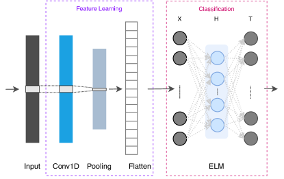
Figure 1: CNN-ELM model

III-D CNN-ELM Indoor Localisation

Wi-Fi fingerprinting is a popular indoor positioning technique given that APs and/or Wi-Fi routers are already deployed in both indoor and outdoor environments, avoiding deployment costs. Generally, this technique is divided into two phases. The off-line phase, where different RSS values are collected in known reference points in order to form the radio map. The formed radio map is divided into two or three sub-datasets to train ML models to predict or classify the incoming fingerprints in the online phase. In the on-line phase, the user device obtains some RSS values (unknown position) which are used to predict the user location.

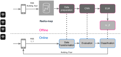
Figure 2: Wi-Fi fingerprinting and CNN-ELM model

Figure 2 shows the workflow at the off-line and on-line stages of the proposed CNN-ELM model for smartphone-based Wi-Fi fingerprinting. Since the proposed classification model for building and floor estimation does not require many computational resources in both off-line and on-line phase of Wi-Fi fingerprinting, it can be used in power-constrained devices, servers with limited capabilities, and IPS with many concurrent users.

IV Experiments and Results

This section provides a general description of the experiment setup, datasets used, and main results obtained in this research work.

IV-A Experiment setup

The experiments were performed using twelve public Wi-Fi fingerprint datasets: UJIIndoorLoc (UJI 1–2) [19], LIB 1–2 [27] (Universitat Jaume I); TUT 1–7 [28, 29, 30, 31, 32, 33] (Tampere University) and UTSIndoorLoc [18] (University of Technology Sydney). These datasets are diverse and have been collected using multiple devices and in differing scenarios, such as libraries and universities. The proposed evaluation setup allows us to obtain a generalized assessment and meaningful results as presented by [34, 23].

All the experiments have been carried out using a computer with the following characteristics: Intel® Core™ i7-8700T @ 2.40 GHz and 16 GB of RAM, the operating system is Fedora Linux 32, and the software used is python 3.9.

TABLE II: Datasets Parameters

Dataset	$\lvert\mathcal{T}_{TR}\rvert$	$\lvert\mathcal{T}_{TE}\rvert$	$\lvert\mathcal{A}\rvert$	$\lvert L\rvert$	DB Type	Data Rep.
LIB 1	576	3120	174	105	MF	Powed
LIB 2	576	3120	197	105	MF	Powed
TUT 1	1476	490	309	75	MF	Powed
TUT 2	584	176	354	160	MF	Powed
TUT 3	697	3951	992	235	MF	Powed
TUT 4	3951	697	992	275	MF	Powed
TUT 5	446	982	489	195	MF	Powed
TUT 6	3116	7269	652	450	MF	Powed
TUT 7	2787	6504	801	200	MF	Powed
UJI 1	19861	1111	520	530	MB-MF	Powed
UJI 2	20972	5179	520	215	MB-MF	Powed
UTS 1	9108	388	589	275	MF	Powed

Table II summarizes the characteristics of each dataset. $\lvert\mathcal{T}_{TR}\rvert$ represents the number of samples in the training dataset, $\lvert\mathcal{T}_{TE}\rvert$ is the number of samples in the test dataset, $\lvert\mathcal{A}\rvert$ represents the number of APs, DB Type shows if the dataset is multi-building (MB), multi-floor (MF) or both. $\lvert L\rvert$ represent the number of hidden neurons used in the ELM.

$k$-NN has been chosen as the baseline with $k=1$, and euclidean distance as the main distance metric. The $k$-NN has been implemented using the KNeighborsClassifier class of sklearn library. Furthermore, CNNLoc [18], ELM, and AFARLS have been used to compare the performance of the proposed CNN-ELM model in terms of building hit rate ($\zeta_{b}$), floor hit rate ($\zeta_{f}$), prediction time ($\delta_{tr}$) and training time ($\delta_{te}$). Thus, their normalized values $\tilde{\zeta}_{b}$, $\tilde{\zeta}_{f}$, $\tilde{\delta}_{tr}$ and $\tilde{\delta}_{te}$ are used to compare the results within the differing approaches. Given that $k$-NN does not have any training stage, the CNNLoc training time was taken as baseline.

In order to run the CNNLoc approach, the training dataset was divided into training and validation datasets. First, the training dataset was divided into buildings (if dataset is multi-building) and then into floors. From each floor in each building, $10\%$ of fingerprints were randomly taken for validation.

To choose the number of hidden nodes in the ELM network, the experiment was first run using five hidden neurons in the hidden layer and it was then increased in steps of five. The regularization term ($c$) in Eq. 8 takes the values: $1$ (TUT 7), $0.1$ (TUT 1, TUT 6, UJI 1), $0.05$ (LIB 1, TUT 3, TUT 4) and $0.01$ (LIB 2, TUT 2, TUT 5, UJI 2, UTS 1). Finally, the number of neurons found to provide a good general performance were selected. Given the random components of CNN-ELM, the random generation was seeded to ensure replicability.

The feature learning block was developed using Keras backend for low-level tasks in order to reduce the load and computational time during training and testing.

IV-B Results

Table III shows the comparison between the results obtained by AFARLS [22] and the proposed CNN-ELM in UJI 1 and TUT 3, reveling that CNN-ELM provides a slightly lower floor hit rate ($<4\%$) than AFARLS in both datasets. However, the number of hidden neurons used in our ELM is significantly lower –more than $47\%$– than in AFARLS. Similarly, our proposed method provided significantly lower training and testing times, but $\delta_{tr}$ and $\delta_{te}$ reported in [22] include the 2D positioning error, which is not incorporated in this research. In the case of building hit rate, its accuracy was not affected.

TABLE III: Datasets Parameters

Approach	Database	Parameters	$\zeta_{b}$	$\zeta_{f}$	$\delta_{tr}$	$\delta_{te}$
			$[\%]$	$[\%]$	$[$\sec$]$	$[$\sec$]$
AFARLS [22]	UJI 1	$L=1000$	$100\%$	$95.41\%$	$84.68$	$0.21$
	TUT 3	$L=1000$	$-$	$94.18\%$	$2.40$	$0.57$
CNN-ELM	UJI 1	$L=530$	$100\%$	$92.26\%$	$0.26$	$0.03$
	TUT 3	$L=235$	$-$	$93.27\%$	$0.22$	$0.10$

TABLE IV: Comparison among the 1-NN baseline, CNNLoc, ELM and CNN-ELM.

	Baseline 1-NN								CNNLoc [18]				ELM				CNN-ELM
Database	$\zeta_{b}$	$\zeta_{f}$	$\delta_{tr}$	$\delta_{te}$	$\tilde{\zeta}_{b}$	$\tilde{\zeta}_{f}$	$\tilde{\delta}{tr}$	$\tilde{\delta}_{te}$	$\tilde{\zeta}_{b}$	$\tilde{\zeta}_{f}$	$\tilde{\delta}{tr}$	$\tilde{\delta}_{te}$	$\tilde{\zeta}_{b}$	$\tilde{\zeta}_{f}$	$\tilde{\delta}{tr}$	$\tilde{\delta}_{te}$	$\tilde{\zeta}_{b}$	$\tilde{\zeta}_{f}$	$\tilde{\delta}{tr}$	$\tilde{\delta}_{te}$
	$[\%]$	$[\%]$	$[$\sec$]$	$[$\sec$]$	$[-]$	$[-]$	$[-]$	$[-]$	$[-]$	$[-]$	$[-]$	$[-]$	$[-]$	$[-]$	$[-]$	$[-]$	$[-]$	$[-]$	$[-]$	$[-]$
LIB1	-	99.20	-	0.1328	-	1	-	1	-	1.0039	1	3.2084	-	1.0042	0.0105	0.2647	-	1.0074	0.0897	0.7417
LIB2	-	99.81	-	0.0972	-	1	-	1	-	0.9830	1	4.7390	-	0.9888	0.0119	0.4769	-	0.9929	0.0244	0.4777
TUT1	-	90.82	-	0.0559	-	1	-	1	-	0.9753	1	8.1930	-	0.9820	0.0042	0.5141	-	1.0045	0.0066	0.5328
TUT2	-	94.32	-	0.0239	-	1	-	1	-	0.9759	1	8.0924	-	0.9518	0.0120	0.9895	-	0.9760	0.0147	1.1848
TUT3	-	91.60	-	0.1949	-	1	-	1	-	0.9710	1	3.6773	-	1.0177	0.0138	0.4998	-	1.0182	0.0156	0.5218
TUT4	-	94.69	-	0.1754	-	1	-	1	-	0.9606	1	1.4059	-	0.9954	0.0022	0.1661	-	1.0121	0.0042	0.1720
TUT5	-	96.84	-	0.0355	-	1	-	1	-	1.0126	1	7.9418	-	1.0074	0.0121	0.7801	-	1.0147	0.0201	0.7493
TUT6	-	99.66	-	0.8479	-	1	-	1	-	1.0011	1	1.3660	-	0.9996	0.0033	0.0765	-	0.9988	0.0079	0.1562
TUT7	-	98.36	-	0.8233	-	1	-	1	-	0.9712	1	1.1628	-	0.9919	0.0029	0.0651	-	0.9922	0.0052	0.0795
UJI1	100	92.17	-	0.6946	1	1	-	1	0.9973	1.0322	1	0.9338	0.9991	0.9375	0.0007	0.0395	1	1.0010	0.0010	0.0488
UJI2	100	91.31	-	2.9602	1	1	-	1	1	0.9444	1	0.2622	0.9996	0.9854	0.0005	0.0163	1	1.0173	0.0011	0.0141
UTS1	-	94.07	-	0.1541	-	1	-	1	-	0.9151	1	3.4835	-	0.9890	0.0011	0.1840	-	1.0137	0.0019	0.3950
Avg.	100	95.24	-	0.52	1	1	-	1	0.9987	0.9789	1	3.7055	0.9994	0.9876	0.0063	0.3394	1	1.0041	0.0160	0.4228

Table IV shows the results obtained with $k$-NN, CNNLoc, ELM, and the proposed CNN-ELM. The baseline provides $100\%$ in the building hit rate in UJI 1 and UJI 2. The average accuracy in the floor hit rate is $95.24\%$, and the average classification time is $0.52\text{\,}\mathrm{s}$. If we compare CNNLoc with the baseline, we see that the building hit rate slightly decreased in the UJI 1 dataset. Similarly, the average floor hit rate decreased by $2\%$ approximately. Nevertheless, the CNNLoc performance is better than the baseline in four datasets (LIB 1, TUT 5, TUT 6, and UJI 1). Surprisingly, the prediction time increased threefold compared with the baseline.

The ELM network provides a better classification performance than CNNLoc, but it is still lower than the baseline. In the case of LIB 1, TUT 3 and TUT 7, the floor hit rates are slightly higher than the baseline (by less than $1\%$). There is a minimal reduction in the building hit rate in the UJI 1 and UJI 2 datasets. The training and testing time is, however, considerably lower in relation to the $k$-NN and CNNLoc in all datasets. For instance, the average testing time was reduced by more than $66\%$ in comparison with the baseline.

In the case of the CNN-ELM, it has the same classification accuracy as the baseline ($1$ in the building hit rate and $1.0041$ in the floor hit rate). Compared to the CNNLoc, and ELM network, the classification accuracy of the CNN-ELM increases by more than $2\%$ on average. In spite of the fact that there is a slight increment in the training and testing time, this is offset by improved classification accuracy when we compare our approach with ELM network. Thus, the average training time is more than sixty times faster than the CNNLoc, the average testing time was reduced by almost $58\%$ in contrast with baseline, and it is just $25\%$ higher than the ELM network.

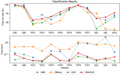
Figure 3: Classification results

Figure 3 shows the classification results (without normalization) in terms of floor hit rate (top) and testing time (bottom). The minimum floor hit rate achieved with CNN-ELM is greater than $91\%$ in the TUT 1 dataset, and the maximum is almost $100\%$ in LIB 1. Finally, CNN-ELM provides better floor detection rate in UJI 2 and UTS 1, the largest datasets in terms of number of buildings and floors.

V Discussion

In the previous section we compared four different approaches; $k$-NN, CNNLoc, ELM and, briefly, AFARLS with our approach (CNN-ELM) in Table III. Although, the classification accuracy with CNN-ELM model is not as high as AFARLS in the case of the UJI 1 (UJIIndoorLoc in [22]) and TUT 3 (Tampere in [22]) datasets. The training and testing time is significantly lower than AFARLS.

We have to consider that data preprocessing is fundamental prior to applying any machine learning model. This case is not the exception, powed data representation and data normalization technique allowed to enhance the dataset’s characteristics. These two techniques were essential to achieve better classification accuracy and processing time (training and testing time).

Similarly, code and algorithm optimization play an important role in offering fast training and testing time. Thus, if additional calculations are done during the prediction time, the time response will increase along with the computational load. An inefficient implementation may raise scalability problem when deploying an Indoor Positioning system.

As expected, the feature learning block allowed us to extract a high level of characteristics from the radio map in such a manner that the ELM network can process that information more efficiently. Thus, with minimal training time, the network can provide high levels of accuracy in line with to complex networks such as CNNLoc or AFARLS.

VI Conclusions

In this paper, we present a lightweight ensemble CNN-ELM model for building and floor indoor-positioning classification.

We have performed a comprehensive evaluation using twelve diverse datasets and compared against three known models from the literature (CNNLoc, $k$-NN and ELM). Two of these datasets were also compared against AFARLS approach.

Although the CNN-ELM network is simple, it has been capable of providing similar or better performance than complex machine learning models in short run times. Thus, the average testing time was $58\%$ faster than the baseline model based on $1$-NN, providing almost the same positioning error. Compared with the AFARLS approach, the classification accuracy of CNN-ELM was less than $4\%$ worse. However, the number of hidden neurons used in the ELM was $\approx 47\%$ less than the number of hidden neurons used in the AFARLS architecture in the datasets analysed. This makes our proposal also lighter to operate in terms of memory requirements.

Future work will include analysis of using the CNN-ELM network to provide 2D and 3D positioning estimation as well as new optimisation techniques.

References

- [1] Matteo D’Aloia et al. “IoT Indoor Localization with AI Technique” In 2020 IEEE International Workshop on Metrology for Industry 4.0 IoT, 2020, pp. 654–658 DOI: 10.1109/MetroInd4.0IoT48571.2020.9138275
- [2] Alexander E.I Brownlee et al. “Exploring the Accuracy – Energy Trade-off in Machine Learning” In 2021 IEEE/ACM International Workshop on Genetic Improvement, 2021, pp. 11–18 DOI: 10.1109/GI52543.2021.00011
- [3] Joaquín Torres-Sospedra et al. “New Cluster Selection and Fine-grained Search for k-Means Clustering and Wi-Fi Fingerprinting” In 2020 International Conference on Localization and GNSS (ICL-GNSS), 2020, pp. 1–6 DOI: 10.1109/ICL-GNSS49876.2020.9115419
- [4] Weixing Xue et al. “Improved Clustering Algorithm of Neighboring Reference Points Based on KNN for Indoor Localization” In 2018 Ubiquitous Positioning, Indoor Navigation and LBS, 2018 DOI: 10.1109/UPINLBS.2018.8559874
- [5] Wenhua Shao et al. “Indoor Positioning Based on Fingerprint-Image and Deep Learning” In IEEE Access 6, 2018, pp. 74699–74712 DOI: 10.1109/ACCESS.2018.2884193
- [6] Minh Tu Hoang et al. “Recurrent Neural Networks for Accurate RSSI Indoor Localization” In IEEE Internet of Things Journal 6.6, 2019, pp. 10639–10651 DOI: 10.1109/JIOT.2019.2940368
- [7] Guang-Bin Huang, Qin-Yu Zhu and Chee-Kheong Siew “Extreme learning machine: Theory and applications” In Neurocomputing 70, 2006, pp. 489–501 DOI: https://doi.org/10.1016/j.neucom.2005.12.126
- [8] Hualong Yu et al. “Active Learning From Imbalanced Data: A Solution of Online Weighted Extreme Learning Machine” In IEEE Transactions on Neural Networks and Learning Systems 30.4, 2019, pp. 1088–1103 DOI: 10.1109/TNNLS.2018.2855446
- [9] Meiyi Li, Weibiao Cai and Qingshuai Sun “Extreme Learning Machine for Regression Based on Condition Number and Variance Decomposition Ratio” In Proceedings of 2018 International Conference on Mathematics and Artificial Intelligence, 2018, pp. 42–45 DOI: 10.1145/3208788.3208794
- [10] Jichao Chen et al. “Unsupervised feature selection based extreme learning machine for clustering” In Neurocomputing 386, 2020, pp. 198–207 DOI: https://doi.org/10.1016/j.neucom.2019.12.065
- [11] Liyanaarachchi Lekamalage Chamara Kasun et al. “Dimension Reduction With Extreme Learning Machine” In IEEE Transactions on Image Processing 25.8, 2016, pp. 3906–3918 DOI: 10.1109/TIP.2016.2570569
- [12] Xiaoxuan Lu et al. “Robust Extreme Learning Machine With its Application to Indoor Positioning” In IEEE Transactions on Cybernetics 46, 2015, pp. 1–1 DOI: 10.1109/TCYB.2015.2399420
- [13] Zheng Wu et al. “A Fast and Resource Efficient Method for Indoor Positioning Using Received Signal Strength” In IEEE Transactions on Vehicular Technology 65.12, 2016, pp. 9747–9758 DOI: 10.1109/TVT.2016.2530761
- [14] Darwin Quezada-Gaibor et al. “Supplementary material ”Lightweight Hybrid CNN-ELM Model for Multi-building and Multi-floor Classification”” Zenodo, 2022 DOI: 10.5281/zenodo.6347465
- [15] P. Mpeis et al. “The Anyplace 4.0 IoT Localization Architecture” In 2020 21st IEEE International Conference on Mobile Data Management (MDM), 2020, pp. 218–225
- [16] FIND “FIND: The Framework for Internal Navigation and Discovery” Last accessed 10 March 2022, 2022 URL: https://www.internalpositioning.com
- [17] Indoo.rs “Indoor Mapping: Transform your analog floor plan into a digital indoor map to visualize Points of Interest, people and objects.” Last accessed 10 March 2022, 2022 URL: https://indoo.rs/
- [18] Xudong Song et al. “CNNLoc: Deep-Learning Based Indoor Localization with WiFi Fingerprinting” In 2019 IEEE SmartWorld, Ubiquitous Intelligence Computing, Advanced Trusted Computing, Scalable Computing Communications, Cloud Big Data Computing, Internet of People and Smart City Innovation, 2019, pp. 589–595 DOI: 10.1109/SmartWorld-UIC-ATC-SCALCOM-IOP-SCI.2019.00139
- [19] Joaquín Torres-Sospedra et al. “UJIIndoorLoc: A new multi-building and multi-floor database for WLAN fingerprint-based indoor localization problems” In 2014 International Conference on Indoor Positioning and Indoor Navigation, 2014, pp. 261–270 DOI: 10.1109/IPIN.2014.7275492
- [20] Elena Simona Lohan et al. “Wi-Fi Crowdsourced Fingerprinting Dataset for Indoor Positioning” In Data 2.4, 2017 DOI: 10.3390/data2040032
- [21] Han Zou et al. “A Fast and Precise Indoor Localization Algorithm Based on an Online Sequential Extreme Learning Machine” In Sensors 15.1, 2015, pp. 1804–1824 DOI: 10.3390/s150101804
- [22] Lijun Lian et al. “Improved Indoor positioning algorithm using KPCA and ELM” In 2019 11th International Conference on Wireless Communications and Signal Processing (WCSP), 2019, pp. 1–5 DOI: 10.1109/WCSP.2019.8928106
- [23] Joaquín Torres-Sospedra et al. “A Comprehensive and Reproducible Comparison of Clustering and Optimization Rules in Wi-Fi Fingerprinting” In IEEE Transactions on Mobile Computing 21.3, 2022, pp. 769–782 DOI: 10.1109/TMC.2020.3017176
- [24] Mai Ibrahim, Marwan Torki and Mustafa ElNainay “CNN based Indoor Localization using RSS Time-Series” In 2018 IEEE Symposium on Computers and Communications (ISCC), 2018, pp. 01044–01049 DOI: 10.1109/ISCC.2018.8538530
- [25] Xiaoxuan Lu et al. “Robust Extreme Learning Machine With its Application to Indoor Positioning” In IEEE Transactions on Cybernetics 46, 2016, pp. 194–205
- [26] Radu Dogaru and Ioana Dogaru “BCONV - ELM: Binary Weights Convolutional Neural Network Simulator based on Keras/Tensorflow, for Low Complexity Implementations” In 2019 6th International Symposium on Electrical and Electronics Engineering (ISEEE), 2019, pp. 1–6 DOI: 10.1109/ISEEE48094.2019.9136102
- [27] Germán Martín Mendoza-Silva et al. “Long-Term WiFi Fingerprinting Dataset for Research on Robust Indoor Positioning” In Data 3.1, 2018
- [28] S. Shrestha, J. Talvitie and E.. Lohan “Deconvolution-based indoor localization with WLAN signals and unknown access point locations”, 2013 URL: http://www.cs.tut.fi/tlt/pos/MEASUREMENTS˙WLAN˙FOR˙WEB.zip
- [29] Alireza Razavi, Mikko Valkama and Elena-Simona Lohan “K-Means Fingerprint Clustering for Low-Complexity Floor Estimation in Indoor Mobile Localization” In IEEE Globecom Workshops (GC Wkshps), 2015
- [30] Andrei Cramariuc, Heikki Huttunen and Elena Simona Lohan “Clustering benefits in mobile-centric WiFi positioning in multi-floor buildings” In 2016 International Conference on Localization and GNSS, 2016
- [31] Elena-Simona Lohan et al. “Wi-Fi Crowdsourced Fingerprinting Dataset for Indoor Positioning” In MDPI Data 2.4 MDPI, 2017
- [32] Philipp Richter, Elena Simona Lohan and Jukka Talvitie “WLAN (WiFi) RSS database for fingerprinting positioning”, 2018 URL: https://zenodo.org/record/1161525
- [33] Lohan “Additional TAU datasets for Wi-Fi fingerprinting- based positioning” Zenodo, 2020 URL: https://doi.org/10.5281/zenodo.3819917
- [34] Nicola Saccomanno, Andrea Brunello and Angelo Montanari “What You Sense Is Not Where You Are: On the Relationships between Fingerprints and Spatial Knowledge in Indoor Positioning” In IEEE Sensors Journal, 2021 DOI: 10.1109/JSEN.2021.3070098