Dirichlet Proportions Model for Hierarchically Coherent Probabilistic Forecasting

Abstract

Probabilistic, hierarchically coherent forecasting is a key problem in many practical forecasting applications – the goal is to obtain coherent probabilistic predictions for a large number of time series arranged in a pre-specified tree hierarchy. In this paper, we present an end-to-end deep probabilistic model for hierarchical forecasting that is motivated by a classical top-down strategy. It jointly learns the distribution of the root time series, and the (dirichlet) proportions according to which each parent time-series is split among its children at any point in time. The resulting forecasts are naturally coherent, and provide probabilistic predictions over all time series in the hierarchy. We experiment on several public datasets and demonstrate significant improvements of up to 26% on most datasets compared to state-of-the-art baselines. Finally, we also provide theoretical justification for the superiority of our top-down approach compared to the more traditional bottom-up modeling.

1 Introduction

A central problem in multivariate forecasting is the need to forecast a large group of time series arranged in a natural hierarchical structure, such that time series at higher levels of the hierarchy are aggregates of time series at lower levels. For example, hierarchical time series are common in retail forecasting applications [Fildes et al., 2019], where the time series may capture retail sales of a company at different granularities such as item-level sales, category-level sales, and department-level sales. In electricity demand forecasting [Van Erven and Cugliari, 2015], the time series may correspond to electricity consumption at different granularities, starting with individual households, which could be progressively grouped into city-level, and then state-level consumption time-series. The hierarchical structure among the time series is usually represented as a tree, with leaf-level nodes corresponding to time series at the finest granularity, while higher-level nodes represent coarser-granularities and are obtained by aggregating the values from its children nodes.

Since businesses usually require forecasts at various different granularities, the goal is to obtain accurate forecasts for time series at every level of the hierarchy. Furthermore, to ensure decision-making at different hierarchical levels are aligned, it is essential to generate predictions that are coherent [Hyndman et al., 2011] with respect to the hierarchy, that is, the forecasts of a parent time-series should be equal to the sum of forecasts of its children time-series. For example, the sum of the sales predictions for each shoe style should equal the sales prediction for the shoe category . Finally, to facilitate better decision making, there is an increasing shift towards probabilistic forecasting [Berrocal et al., 2010, Gneiting and Katzfuss, 2014]; that is, the forecasting model should quantify the uncertainty in the output and produce a probability distribution, instead of a single point estimate, for predictions.

In this paper, we address the problem of obtaining coherent probabilistic forecasts for large-scale hierarchical time series. While there has been a plethora of work on multivariate forecasting, there is significantly limited research on multivariate forecasting for hierarchical time series that satisfy the requirements of both hierarchical coherence and probabilistic predictions.

There are numerous recent works on deep neural network-based multivariate forecasting [Salinas et al., 2020, Oreshkin et al., 2019, Rangapuram et al., 2018, Benidis et al., 2020, Sen et al., 2019, Olivares et al., 2022a], including probabilistic multivariate forecasting [Salinas et al., 2019, Rasul et al., 2021] and even graph neural network(GNN)-based models for forecasting on time series with graph-structure correlations [Bai et al., 2020, Cao et al., 2020, Yu et al., 2017, Li et al., 2017]. However, none of these works ensure coherent predictions for hierarchical time series.

On the other hand, several papers specifically address hierarchically-coherent forecasting  [Hyndman et al., 2016, Taieb et al., 2017, Van Erven and Cugliari, 2015, Hyndman et al., 2016, Ben Taieb and Koo, 2019, Wickramasuriya et al., 2015, 2020, Mancuso et al., 2021, Abolghasemi et al., 2019], based on the idea of reconciliation. This involves a two-stage process where the first stage generates independent (possibly incoherent) univariate base forecasts, and is followed by a second reconciliation stage that adjusts these forecasts using the hierarchy structure, to finally obtain coherent predictions. These approaches are usually disadvantaged in terms of using the hierarchical constraints only as a post-processing step, and not during generation of the base forecasts. Furthermore, with the exception of Taieb et al. [2017], which is a two-stage reconciliation-based model for coherent probabilistic hierarchical forecasting, most of these approaches cannot directly handle probabilistic forecasts.

More recently, there has been some work( Rangapuram et al. [2021], Han et al. [2021a]) that propose single-stage, end-to-end deep neural architectures that directly produce hierarchically-coherent (or approximately coherent) probabilistic forecasts without a need for a post-processing step.

In this paper, we present an alternate approach to end-to-end deep probabilistic forecasting for hierarchical time series, motivated by a classical method that has not received much recent attention: top-down forecasting. The basic idea is to first model the top-level forecast in the hierarchy tree, along with the ratios or proportions according to how the top level forecasts should be distributed among the children time-series in the hierarchy. The resulting predictions are naturally coherent. Early top-down approaches were non-probabilistic, and were rather simplistic in terms of modeling the proportions; for example, by separately modeling the top-level forecast, and then deriving the proportions from historical averages [Gross and Sohl, 1990], or from independently generated (incoherent) forecasts of each time-series from another model [Athanasopoulos et al., 2009]. In this paper, we showcase how modeling both the top-level forecast and the proportions jointly through a single-stage deep probabilistic model can obtain state-of-the-art results for probabilistic, hierarchically-coherent forecasts.

Crucially, our proposed model (and indeed all top-down approaches for forecasting) relies on the intuition that the top level time series in a hierarchy is usually much less noisy and less sparse, and hence much easier to predict. Furthermore, it might be easier to predict proportions (that are akin to scale-free normalized time-series) at the lower level nodes than the actual time series themselves.

Our approach involves learning a single end-to-end deep model to jointly model “families“, consisting of a parent and its children timeseries, and predict both the parent timeseries and the proportions along which it is disaggregated among its children. We use a Dirichlet distribution [Olkin and Rubin, 1964] to model the distribution of proportions for each parent-children family in the hierarchy. The parameters of the Dirichlet distribution for each family is obtained from an MLP (Multi Layer Perceptron) based encoder-decoder model with multi-headed self-attention [Vaswani et al., 2017], that is jointly learnt from the whole dataset.

We validate our model against state-of-the art probabilistic hierarchical forecasting baselines on six public datasets, and demonstrate significant gains using our approach, outperforming the baselines on most datasets with improvements of up to 26% in terms of CRPS scores.

Additionally, we theoretically analyze the advantage of the top-down approach (over a bottom-up approach) in a simplified regression setting for hierarchical prediction, and thereby provide theoretical justification for our top-down model. Specifically, we prove that for a $2$-level hierarchy of $d$-dimensional linear regression with a single root node and $K$ children nodes, the excess risk of the bottom-up approach is $\min(K,d)$ time bigger than the one of the top-down approach in the worst case. This validates our intuition that it is easier to predict proportions than the actual values.

2 Background

Hierarchical forecasting is a multivariate forecasting problem, where we are given a set of $N$ univariate time-series (each having $T$ time points) that satisfy linear aggregation constraints specified by a predefined hierarchy. More specifically, the data can be represented by a matrix $\bm{{Y}}\in\mathbb{R}^{T\times N}$, where ${\bm{y}}^{(i)}$ denotes the $T$ values of the $i$-th time series, ${\bm{y}}_{t}$ denotes the values of all $N$ time series at time $t$, and $y_{t,i}$ the value of the $i$-th time series at time $t$. We will assume that $y_{i,t}\geq 0$, which is usually the case in all retail demand forecasting datasets (and is indeed the case in all public hierarchical forecasting benchmarks [Wickramasuriya et al., 2015]). We compactly denote the $H$-step history of $\bm{{Y}}$ by $\bm{{Y}}_{\mathcal{H}}=[{\bm{y}}_{t-H},\cdots,{\bm{y}}_{t-1}]^{\top}\in\mathbb{R}^{H\times N}$ and the $H$-step history of ${\bm{y}}^{(i)}$ by ${\bm{y}}_{\mathcal{H}}^{(i)}=[{\bm{y}}_{t-H}^{(i)},\cdots,{\bm{y}}_{t-1}^{(i)}]\in\mathbb{R}^{H}$. Similarly we can define the $F$-step future as $\bm{{Y}}_{\mathcal{F}}=[{\bm{y}}_{t},\cdots,{\bm{y}}_{t+F-1}]^{\top}\in\mathbb{R}^{F\times N}$. We use the $\hat{\cdot}$ notation to denote predicted values, and the ${\cdot}^{\top}$ notation to denote the transpose. We denote the matrix of external covariates like holidays etc by $\bm{{X}}\in\mathbb{R}^{T\times D}$, where the $t$-th row denotes the $D$-dimensional feature vector at the $t$-th time step. For simplicity, we assume that the features are shared across all time series. We define $\bm{{X}}_{\mathcal{H}}$ and $\bm{{X}}_{\mathcal{F}}$ similarly. The $\hat{\cdot}$ notation will be used to denote predicted values, for instance $\hat{\bm{{Y}}}_{\mathcal{F}}$ denotes the prediction in the future. We will also use numpy tensor notation i.e $\bm{{X}}[i:j,r:c]$ would denote the sub-matrix in rows $\{i,i+1,\cdots,j-1\}$ and columns $\{r,r+1,\cdots c-1\}$. Further, using $:$ would denote selecting all rows (or columns) depending on the axis.

Hierarchy.  The $N$ time series are arranged in a tree hierarchy, with $m$ leaf time-series, and $k=N-m$ non-leaf (or aggregated) time-series that can be expressed as the sum of its children time-series, or alternatively, the sum of the leaf time series in its sub-tree. Let ${\bm{b}}_{t}\in\mathbb{R}^{m}$ be the values of the $m$ leaf time series at time $t$, and ${\bm{r}}_{t}\in\mathbb{R}^{k}$ be the values of the $k$ aggregated time series at time $t$. The hierarchy is encoded as an aggregation matrix $\bm{{R}}\in\{0,1\}^{k\times m}$ , where an entry $R_{ij}$ is equal to 1 if the $i$-th aggregated time series is an ancestor of the $j$-th leaf time series in the hierarchy tree, and 0 otherwise. We therefore have the aggregation constraints ${\bm{r}}_{t}=\bm{{R}}{\bm{b}}_{t}$ or ${\bm{y}}_{t}=[{\bm{r}}_{t}^{\top}~{}~{}{\bm{b}}_{t}^{\top}]^{\top}=\bm{{S}}{\bm{b}}_{t}$ where $\bm{{S}}^{T}=[\bm{{R}}^{\top}|\bm{{I}}_{m}]$. Here, $\bm{{I}}_{m}$ is the $m\times m$ identity matrix. Such a hierarchical structure is ubiquitous in multivariate time series from many domains such as retail, traffic, etc, as discussed earlier. We provide an example tree with its $\bm{{S}}$ matrix in Figure 1. We can extend this equation to the matrix $\bm{{Y}}\in\mathbb{R}^{T\times N}$. Let $\bm{{B}}:=[{\bm{b}}_{1};\cdots;{\bm{b}}_{m}]^{\top}$ be the corresponding leaf time-series values arranged in a $T\times m$ matrix. Then coherence property of $\bm{{Y}}$ implies that $\bm{{Y}}^{\top}=\bm{{S}}\bm{{B}}^{\top}$. Note that we will use $\bm{{B}}_{\mathcal{F}}$ to denote the leaf-time series matrix corresponding to the future time-series in $\bm{{Y}}_{\mathcal{F}}$.

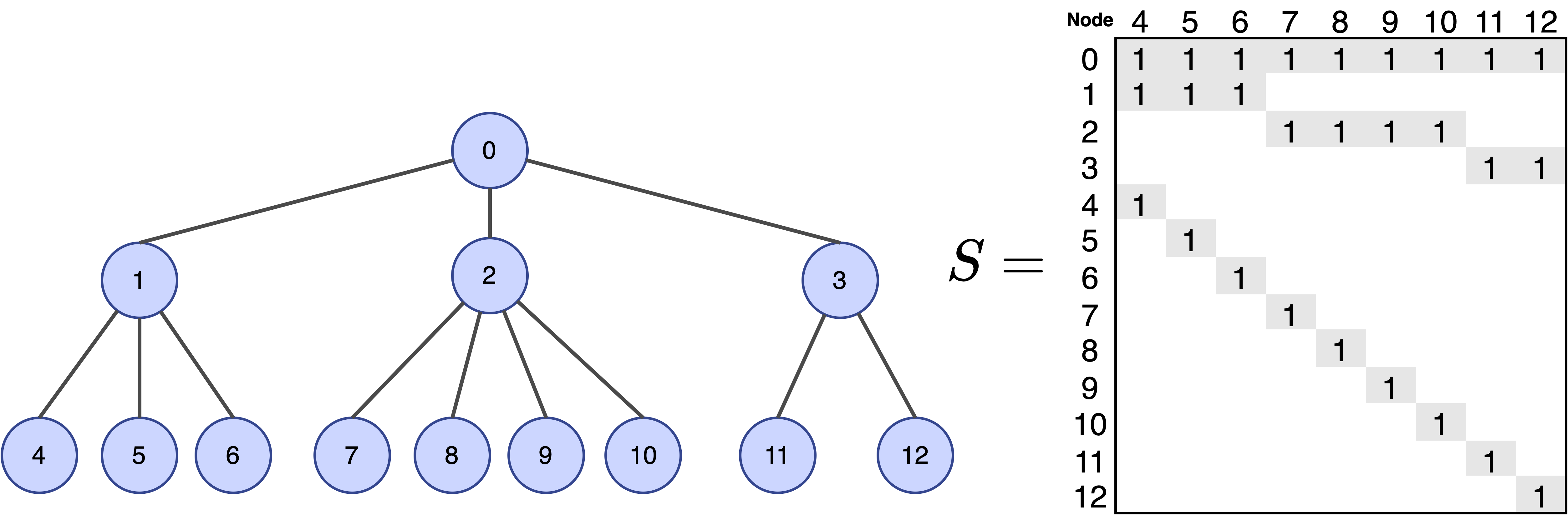
Figure 1: An example of a hierarchy and its corresponding $\bm{{S}}$ matrix. The rows and columns of the matrix are indexed by the corresponding nodes for easier interpretation. The empty cells of the matrix are zeros, and hence omitted from the figure.

Coherency.  Clearly, an important property of hierarchical forecasting is that the forecasts also satisfy the hierarchical constraints $\hat{\bm{{Y}}}^{\top}_{\mathcal{F}}=\bm{{S}}\hat{\bm{{B}}}^{\top}_{\mathcal{F}}$. This is known as the coherence property which has been used in several prior works [Hyndman and Athanasopoulos, 2018, Taieb et al., 2017]. Imposing the coherence property makes sense since the ground truth data $\bm{{Y}}$ is coherent by construction. Coherence is also critical for consistent decision making at different granularities of the hierarchy.

Our objective is to accurately predict the distribution of the future values $\hat{\bm{{Y}}}_{\mathcal{F}}\sim\hat{f}(\bm{{Y}}_{\mathcal{F}})$ conditioned on the history such that any sample $\hat{\bm{{Y}}}\in\mathbb{R}^{F\times N}$ from the predicted distribution $\hat{f}(\bm{{Y}}_{\mathcal{F}})$ satisfies the coherence property. In particular, $\hat{f}$ denotes the density function (multi-variate) of the future values $\bm{{Y}}_{\mathcal{F}}$ conditioned on the historical data $\bm{{X}}_{\mathcal{H}},\bm{{Y}}_{\mathcal{H}}$ and the future features $\bm{{X}}_{\mathcal{F}}$. We omit the conditioning from the expression for readability.

The related work can be broadly classified into (i) Coherent point forecasting that includes but is not limited to approaches like [Hyndman et al., 2011, Van Erven and Cugliari, 2015, Panagiotelis et al., 2020]; (ii) Coherent probabilistic forecasting that includes among others [Taieb et al., 2017, Rangapuram et al., 2021, Olivares et al., 2021] and (iii) Approximately coherent methods like [Mishchenko et al., 2019, Gleason, 2020, Han et al., 2021a, b, Paria et al., 2021]. We include a detailed discussion of related literature in Appendix A.

3 The Model

The basic input data-structure to our model is a family $(p,\mathcal{L}(p))$, where $p$ is a parent node in the hierarchical tree (any non-leaf node) and $\mathcal{L}(p)$ are its children nodes. In Figure 1, the set of nodes $(2,[7,8,9,10])$ denotes a family.

Our main contribution is a shared proportions model that takes in the past data points of a family and predicts (i) the future proportions of the children i.e the fractions by which the parent time-series diaggregates into the children time-series in the future (ii) the future values of the parent. The model is designed to capture dependencies among the children through appropriate applications of attention layers and also propagate information between the parent and the children. We train a single shared global proportions model for all the families in the tree.

Modeling Proportions. Before we describe the model for forecasting the proportions, we need to formally define the children proportions. For a family $(p,\mathcal{L}(p))$ let us define the proportions,

$$a_{s,c}=\frac{y_{s,c}}{\sum_{j\in\mathcal{L}(p)}y_{s,j}},\quad\text{for all }s\in[T],c\in\mathcal{L}(p).$$ (1)

The matrix $\bm{{A}}(p)\in\mathbb{R}^{T\times C}$ denotes the proportions of the children over time, where $C:=|\mathcal{L}(p)|$. We will drop the $p$ in braces when it is clear from context that we are dealing with a particular family $(p,\mathcal{L}(p))$. As in Section 2, we use $\bm{{A}}_{\mathcal{H}}$ and $\bm{{A}}_{\mathcal{F}}$ to denote the historical and future proportions. Also, ${\bm{a}}^{(i)}_{\mathcal{H}}$ will denote the historical proportions for child $i\in\mathcal{L}(p)$ and a similar definition holds for ${\bm{a}}^{(i)}_{\mathcal{F}}$.

We are interested in predicting the distribution of $\bm{{A}}_{\mathcal{F}}$ given historical proportions $\bm{{A}}_{\mathcal{H}}$, the parent’s history ${\bm{y}}^{(p)}_{\mathcal{H}}$ and covariates $\bm{{X}}$. Note that for any $s\in[T]$, the $s$th row of $\bm{{A}}(p)$, ${\bm{a}}_{s}\in\Delta^{C-1}$ (denotes the $(C-1)$-dimensional simplex). Therefore, our predicted distribution should also be a distribution over the simplex for each row. Hence, we use the Dirichlet [Olkin and Rubin, 1964] family to model the output distribution for each row of the predicted proportions, as detailed later.

We choose the simplest possible architectural building blocks for the task at hand: (i) we use a simple MLP (Multi-Layer Perceptron) encoder-decoder model for capturing the temporal dependencies in the proportions of a child (independently of other children) (ii) we use multi-headed attention [Vaswani et al., 2017] to capture dependencies among the children of the family.

Encoder:  We first form an encoding depending on the past for each child,

$${\bm{e}}_{i}\leftarrow\texttt{enc}\mathopen{}\mathclose{{}\left({\bm{a}}_{\mathcal{H}}^{(i)},{\bm{y}}^{(p)}_{\mathcal{H}},\bm{{X}}}\right)$$

where ${\bm{e}}_{i}\in\mathbb{R}^{d_{E}}$ and $d_{E}$ is the encoding dimension. We represent all the children embeddings in the matrix $\bm{{E}}\in\mathbb{R}^{d_{E}\times C}$ such that the $i$-th column of $\bm{{E}}$ is the encoding ${\bm{e}}_{i}$ of the $i$-th child. The MLP encoder, $\texttt{enc}(\cdot)$ is applied independently for each child. Each child’s embedding can also depend on the past of the parent ${\bm{y}}^{(p)}_{\mathcal{H}}$ and the covariates $\bm{{X}}$; thereby drawing information from higher level time-series.

Attention:  Then we apply multi-headed attention to mix the encoded information across the children. The input to the attention is $\bm{{E}}^{\prime}=[\bm{{E}};\mathbf{1}]\in\mathbb{R}^{d_{E}\times(C+1)}$ i.e a dummy column added to the children embeddings (the value of that column will become clear later when we dicuss the parent prediction module). The attention layer is denoted by,

$$\bm{{M}}^{\prime}\leftarrow\texttt{MultiHeadAtt}_{g,l}\mathopen{}\mathclose{{}\left(\bm{{E}}^{\prime}}\right),$$ (2)

where $g$ denotes the number of attention heads and $l$ denotes the number of attention layers. Each attention layer is followed by a fully connected layer with ReLU activation and also equipped with a residual connection (similar to the original model in [Vaswani et al., 2017]). Note that the attention is only applied across the second dimension i.e across the children. The resulting $\bm{{M}}^{\prime}$ is in $\mathbb{R}^{d_{A}\times(C+1)}$ where $d_{A}$ is the value dimension in the attention layers. Let $\bm{{M}}=\bm{{M}}^{\prime}[:,0:C+1]$.

Decoder:  Now that we have mixed the encoded information among the children, we are ready to decode to obtain the predicted distribution of future proportions of the children. The decoding follows the equations:

$$\bm{{D}} =\texttt{dec}(\bm{{M}}),~{}~{}\text{(Output shape: $d_{D}*F\times C$)},$$

$$\bm{{D}}_{\mathcal{F}} =\text{(Reshape of $\bm{{D}}$ into $d_{D}\times F\times C$)},$$

$$\hat{a}_{s,c} =\texttt{dec}_{\mathcal{F}}(\bm{{D}}_{\mathcal{F}}[:,s,c],\bm{{X}}_{\mathcal{F}}[s,:]),~{}~{}\text{(Output shape: 1)}$$

$$\hat{\bm{{A}}}_{\mathcal{F}}~{}\text{is a matrix s.t}~{}\hat{\bm{{A}}}_{\mathcal{F}}[s,c]=\exp(a_{s,c}).$$

In the first equation $\texttt{dec}(\cdot)$ is a MLP decoder with output dimensions $d_{D}*F$ that is applied on the first axis of $\bm{{M}}$. Then the output is reshaped into $\bm{{D}}_{\mathcal{F}}$ such that we have a decoded feature of length $d_{D}$ for all $F$ future time-points and all $C$ children in the family. Then we apply another MLP layer with $\texttt{dec}_{\mathcal{F}}(\cdot)$ with output dimension $1$. For each future time-point $s\in[F]$ and children $c\in C$, $\texttt{dec}_{\mathcal{F}}$ is applied independently on the concatenation of $\bm{{D}}_{\mathcal{F}}[:,s,c]$ and $\bm{{X}}_{\mathcal{F}}[s,:]$ to produce the output parameter $\hat{a}_{s,c}$. Intuitively, this final MLP combines the information in the $d_{D}$ dimensional decoded feature for the children $c$ at future time $s$ along with the future covariates at that time-point to produce the final output. The output for all future time-points and all children are then collected in the matrix $\hat{\bm{{A}}}_{\mathcal{F}}\in\mathbb{R}^{F\times C}$ after passing through the exp. function to ensure positivity.

Loss Function: We would like to output the predicted distribution of the proportions of the children in the family for all future time-steps. Our loss function is designed such that the output from the preceding decoder step $\hat{\bm{{A}}}_{\mathcal{F}}$ can represent such a distribution. Recall that the predicted proportions distributions $\hat{f}(\bm{{A}}_{\mathcal{F}})$ have to be over the simplex $\Delta^{C-1}$ for each time-point. Therefore we model it by the Dirichlet distribution. In fact our final model output $\hat{\bm{{A}}}_{\mathcal{F}}$ represents the parameters of predictive Dirichlet distributions. Specifically, we minimize the loss

$$\ell_{c}(\bm{{A}}_{\mathcal{F}},\hat{\bm{{A}}}_{\mathcal{F}})=-\frac{1}{F}\sum_{s=1}^{F}\texttt{DirLL}\mathopen{}\mathclose{{}\left({\bm{a}}_{s}+\epsilon;\hat{\mathbf{a}}_{s}}\right),$$ (3)

where ${\bm{a}}_{s}$ is the proportion of the children nodes in the family at time $s$ as defined in Equation (1). $\texttt{DirLL}({\bm{a}};\mathbf{\bm{\beta}})$ denotes the log-likelihood of Dirichlet distribution for target ${\bm{a}}$ and parameters $\mathbf{\bm{\beta}}$.

$$\texttt{DirLL}({\bm{a}};\mathbf{\bm{\beta}}):=\sum_{i}(\beta_{i}-1)\log(a_{i})-\log B(\mathbf{\bm{\beta}}),$$ (4)

where $B(\mathbf{\bm{\beta}})$ is the normalization constant. In Eq. (3), we add a small $\epsilon$ to avoid undefined values when the target proportion for some children are zero. Here, $B(\mathbf{\bm{\beta}})=\prod_{i=1}^{C}\Gamma(\beta_{i})/\Gamma(\sum_{i}\beta_{i})$ where $\Gamma(.)$ is the well-known Gamma function that is differentiable. In practice, we use Tensorflow Probability [Dillon et al., 2017] to optimize the above loss function.

Modeling the Parent. The remaining task is to predict the future values of the parent node in a family. Recall that the output of the attention layer $\bm{{M}}^{\prime}$ in Eq. (2) has an extra dimension in the second axis. We will use the output in that dimension as an input to the decoder that predicts the future of the parent. This allows us to distill historical information from the children that might also be useful for predicting the future values of the parent. The decoding for the parent prediction comprises of the following equations:

$$\bm{{P}} =\texttt{dec}^{(p)}(\bm{{M}}[:,-1],{\bm{y}}^{(p)}_{\mathcal{H}})~{}~{}\text{(Output shape: $d_{D}*F$)},$$

$$\bm{{P}}_{\mathcal{F}} =\text{(Reshape of $\bm{{P}}$ into $F\times d_{D}$)},$$

$$\hat{{\bm{p}}}_{s} =\texttt{dec}_{\mathcal{F}}^{(p)}(\bm{{P}}_{\mathcal{F}}[s,:],\bm{{X}}_{\mathcal{F}}[s,:]),~{}~{}\text{(Output shape: 2)}$$

$$\hat{\bm{{P}}}_{\mathcal{F}}~{}\text{is a matrix s.t}~{}\hat{{\bm{p}}}[s,:]=\hat{{\bm{p}}}_{s}.$$

In the first equation we use the MLP decoder to map the last dimension of the attention encoding from the children along with the past of the parent, to the future decoding of shape $d_{D}*F$. The decoding is then reshaped to have shape $F\times d_{D}$. The final parent decoding layer is an MLP $\texttt{dec}_{\mathcal{F}}^{(p)}$ with output dimension $2$ that maps each future time-step’s decoded features $\bm{{P}}_{\mathcal{F}}[s,:]$ along with the covariates at that time-step to the final predicted parameters for that time-step.

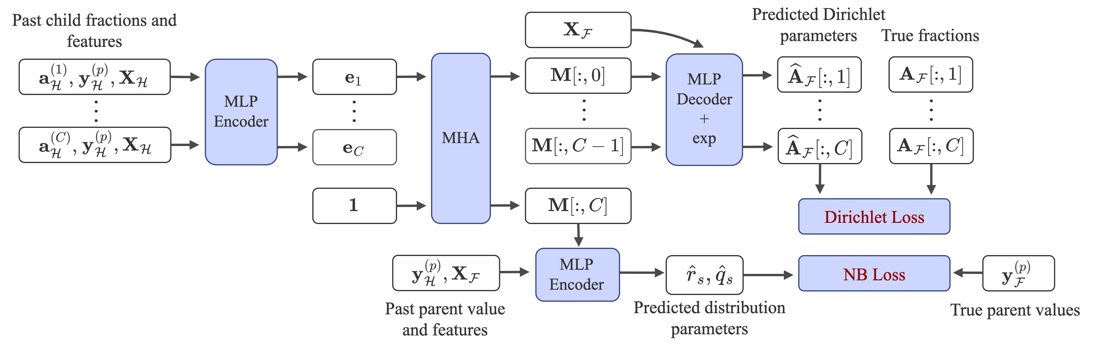
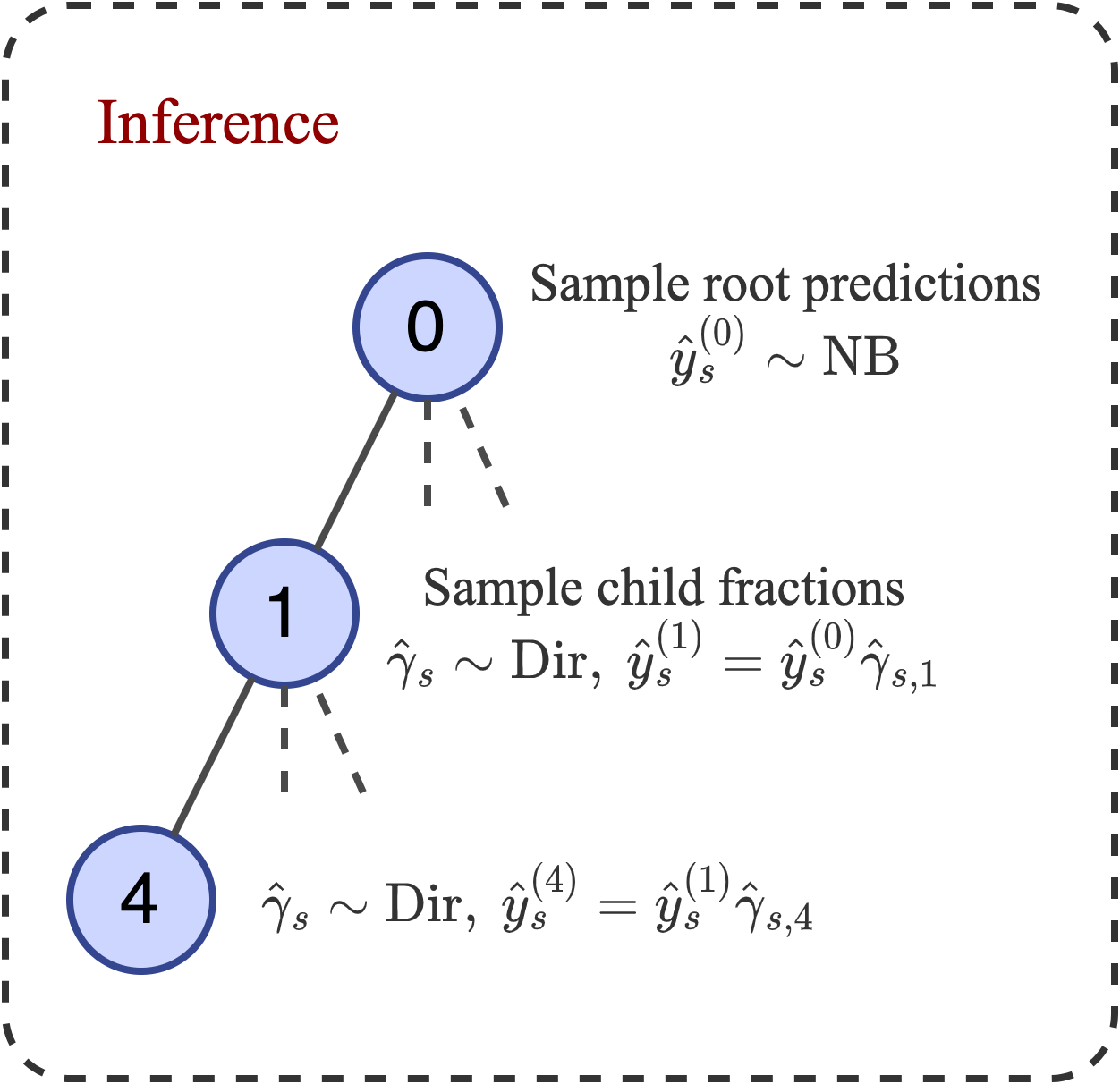
Figure 2: We provide a complete description of the training architecture. MHA denotes multi-head self attention layers. The indices $\{1,\cdots,C\}$ are used to denote the indices of the children of the parent node $p$. During inference, the top level predictions are first sampled from the negative binomial distribution with the predicted parameters $\hat{q}_{s},\hat{r}_{s}$. The children prediction are then successively sampled by first sampling the fractions $\hat{\gamma}_{s}$ from the Dirichlet distribution and then multiplying with the parent sample.

Loss Function. Since we are interested in probabilistic forecasting, we would like to predict the distribution of the parent’s future values. Therefore we will map the output parameters in each future time step ($\hat{{\bm{p}}}_{s}$ for time-step $s\in[F]$) to the parameters of a negative-binomial distribution. The p.m.f of negative binomial distribution with total count $r>0$ and success probability $q\in[0,1]$ is given by,

$$\texttt{NBL}(k;r,q)=\frac{\Gamma(k+r)}{\Gamma(k+1)\Gamma(r)}(1-q)^{k}q^{r}~{}\text{for}~{}k=1,2,\cdots$$ (5)

We first map the predicted parameters from the parent decoder $\hat{{\bm{p}}}_{s}$ to the distribution parameters $\hat{r}_{s},\hat{q}_{s}$ using link functions (designed to keep $(r,q)$ in valid ranges):

$$\hat{r}_{s} =\sigma(\hat{{\bm{p}}}_{s}[0])$$

$$\hat{q}_{s} =\frac{1}{1+\sigma(\hat{{\bm{p}}}_{s}[1])},$$

where $\sigma(x):=(2+x-|x|)/(2-x+|x|)$. Thus $\sigma$ maps $\mathbb{R}\rightarrow\mathbb{R}^{+}$. Finally we minimize the negative log likelihood of observing the actual future values of the parents under the negative binomial distribution formed by the predicted parameters,

$$\ell_{p}({\bm{y}}^{(p)}_{\mathcal{F}},\hat{\bm{{P}}}_{\mathcal{F}})=-\frac{1}{F}\sum_{s=1}^{F}\log\mathopen{}\mathclose{{}\left(\texttt{NBL}(y_{p,s};\hat{r}_{s},\hat{q}_{s})}\right).$$ (6)

We use the negative binomial distribution since a most hierarchical forecasting datasets contain count data that is positive. In such cases, the negative binomial loss has been used with great success in the context of time-series forecasting [Awasthi et al., 2021, Salinas et al., 2020].

The final loss is the summation of the children loss in Eq. (3) and the parent loss in Eq. (6). We provide a full illustration of our model in Figure 2. We refer to our model as DirProp.

Training. We train our model with mini-batch gradient descent where each batch corresponds to different history and future time-intervals of the same family. For example, if the time batch-size is $b$ and we are given a family $(p,\mathcal{L}(p))$ the input proportions that are fed into the model are of shape $b\times H\times C$ and the output distribution parameters for the Dirchlet loss are of shape $b\times F\times C$, where $C=|\mathcal{L}(p)|$. Note that we only need to load all the time-series of a given family into a batch.

Inference. At inference we have to output a representation of the predicted cumulative distribution $\hat{F}(\bm{{Y}}_{\mathcal{F}})$ such that the samples are reconciled as in Section 2. For ease of illustration, we will demonstrate the procedure for one time point $s\in\{1,\cdots,F\}$.

We first sample $\hat{y}_{s}^{(p)}$ from the predictive distribution of the parent for the family containing the root node. For instance, in the tree of Figure 1, this family would be $(0,[1,2,3])$. Then for each family $(p,\mathcal{L}(p))$ in the tree we generate a sample from the Dirchlet distribution with parameters $\hat{\bm{{A}}}_{\mathcal{F}}[s,:]$ that represents a sample of the predicted children proportions for that family. The proportion samples and the root sample can be combined to form a reconciled forecast sample $\hat{{\bm{y}}}_{s}$. We can generate many such samples and then take empirical statistics to form the predictive distribution $\hat{f}(\bm{{Y}}_{s})$, which is by definition reconciled.

4 Theoretical justification for the top-down approach

In this section, we theoretically analyze the advantage of the top-down approach over the bottom-up approach for hierarchical prediction in a simplified setting. Again, the intuition is that the root level time series is much less noisy and hence much easier to predict, and it is easier to predict proportions at the children nodes than the actual values themselves. As a result, combining the root level prediction with the proportions prediction actually yields a much better prediction for the children nodes. Consider a 2-level hierarchy of linear regression problem consisting of a single root node (indexed by $0$) with $K$ children. For each time step $t\in[n]$, a global covariate $\mathbf{x}_{t}\in\mathbb{R}^{d}$ is independently drawn from a Gaussian distribution $\mathbf{x}_{t}\sim\mathcal{N}(0,\Sigma)$, and the value for each node is defined as follows:

• The value of the root node at time $t$ is $y_{t,0}=\theta_{0}^{\top}\mathbf{x}_{t}+\eta_{t}$, where $\eta_{t}\in\mathbb{R}$ is independent of $\mathbf{x}_{t}$, and satisfies $\mathbb{E}[\eta_{t}]=0,\text{Var}[\eta_{t}]=\sigma^{2}$.

• A random $K$-dimensional vector $\mathbf{a}_{t}\in\mathbb{R}^{K}$ is independently drawn from distribution $P$ such that $\mathbb{E}[a_{t,i}]=p_{i}$ and $\text{Var}[a_{t,i}]=s_{i}$, where $a_{t,i}$ is the $i$-th coordinate of $\mathbf{a}_{t}$. For the $i$-th child node, the value of the node is defined as $a_{t,i}\cdot y_{t,0}.$

Notice that for the $i$-th child node, $\mathbb{E}[y_{t,i}|\mathbf{x}_{t}]=p_{i}\theta_{0}^{\top}\mathbf{x}_{t}$, and therefore the $i$-th child node follows from a linear model with coefficients $\theta_{i}\vcentcolon=p_{i}\theta_{0}$.

Now we describe the bottom-up approach and top-down approach and analyze the expected excess risk of them respectively. In the bottom-up approach, we learn a separate linear predictor for each child node seprately. For the $i$-th child node, the ordinary least square (OLS) estimator is

$$\hat{\theta}^{\mathbf{b}}_{i}=\mathopen{}\mathclose{{}\left(\sum_{t=1}^{n}\mathbf{x}_{t}\mathbf{x}_{t}^{\top}}\right)^{-1}\sum_{t=1}^{n}\mathbf{x}_{t}y_{t,i},$$

and the prediction of the root node is simply the summation of all the children nodes.

In the top-down approach, a single OLS linear predictor is first learnt for the root node:

$$\hat{\theta}_{0}^{\mathbf{t}}=\mathopen{}\mathclose{{}\left(\sum_{t=1}^{n}\mathbf{x}_{t}\mathbf{x}_{t}^{\top}}\right)^{-1}\sum_{t=1}^{n}\mathbf{x}_{t}y_{t,0}$$

Then the proportion coefficient $\hat{p}_{i},i\in[K]$ is learnt for each node separately as $\hat{p}_{i}=\frac{1}{n}\sum_{t=1}^{n}y_{t,i}/y_{t,0}$ and the final linear predictor for the $i$th child is $\hat{\theta}^{\mathbf{t}}_{i}=\hat{p}_{i}\hat{\theta}_{0}^{\mathbf{t}}$. Let us define the excess risk of an estimator $\hat{\theta}_{i}$ as $r(\hat{\theta}_{i})=(\hat{\theta}_{i}-\theta_{i})^{\top}\Sigma(\hat{\theta}_{i}-\theta_{i})$. The expected excess risk of both approaches are summarized in the following theorem, proved in Appendix B.1.

Theorem 4.1 (Expected excess risk comparison between top-down and bottom-up approaches).

The total expected excess risk of the bottom-up approach for all the children nodes satisfies

$$\sum_{i=1}^{K}\mathbb{E}[r(\hat{\theta}^{\mathbf{b}}_{i})]\geq\sum_{i=1}^{K}(s_{i}+p_{i}^{2})\frac{d}{n-d-1}\sigma^{2},$$

and the total expected excess risk of the top-down approach satisfies

$$\sum_{i=1}^{K}\mathbb{E}[r(\hat{\theta}^{\mathbf{t}}_{i})]$$

$$=\frac{\sum_{i=1}^{K}{s_{i}}}{n}\theta_{0}^{\top}\Sigma\theta_{0}+\mathopen{}\mathclose{{}\left(\frac{\sum_{i=1}^{K}s_{i}}{n}+\sum_{i=1}^{K}p_{i}^{2}}\right)\frac{d}{n-d-1}\sigma^{2},$$

Applying the theorem to the case where the proportion distribution $\mathbf{a}_{t}$ is drawn from a uniform Dirichlet distribution, we show the excess risk of the traditional bottom-up approach is $\min(K,d)$ times bigger than our proposed top-down approach in the following corollary. A proof of the corollary can be found in Appendix B.2

Corollary 4.2.

Assuming that for each time-step $t\in[n]$, the proportion coefficient $\mathbf{a}_{t}$ is drawn from a $K$-dimensional Dirichlet distribution $\text{Dir}(\alpha)$ with $\alpha_{i}=\frac{1}{K}$ for all $i\in[K]$ and $\theta_{0}^{\top}\Sigma\theta_{0}=\sigma^{2}$, then

$$\frac{\mathbb{E}[\sum_{i=1}^{K}r(\hat{\theta}^{\mathbf{b}}_{i})]}{\mathbb{E}[\sum_{i=1}^{K}r(\hat{\theta}^{\mathbf{t}}_{i})]}=\Omega(\min(K,d)).$$

In Section 5, we show that even the basic topdown approach analyzed in this section outperforms several state of the art methods, thus conforming to our theoretical justification. Our learnt top-down model is a further improvement over the historical fractions.

5 Experiments

We implement our model in Tensorflow [Abadi et al., 2016] and compare our approach with state of the art models for coherent probabilistic forecasting on 6 hierarchical forecasting datasets. We now describe the datasets along with the corresponding forecasting setups.

Datasets. We experiment with two retail forecasting datasets, M5 [M5, 2020] and Favorita [Favorita, 2017]. These are our largest datasets with 3060 and 4471 total time-series in their respective hierarchices. For both these datasets, we use the product hierarchy i.e each leaf time-series corresponds to the sales of an item aggregated across the stores. The other datasets include: Tourism-L [Tourism, 2019, Wickramasuriya et al., 2019] which is a dataset consisting of tourist count data; Labour [of Statistics, 2020], consisting of monthly employment data; Traffic [Cuturi, 2011], consisting of daily occupancy rates of cars on freeways; and Wiki2 [Wiki, 2017], consisting of daily views on Wikipedia articles. For Tourism-L we benchmark on both the (Geo)graphic and (Trav)el history based hierarchy. More details about the dataset and the features used for each dataset can be found in Appendix C and Table 6.

Table 1: We present the normalized metrics WAPE / NRMSE across all levels. We report normalized metrics so that they can be averaged to produce the mean column. All the numbers are averaged over 5 runs. The numbers in bold represent the statistically significant best performances in each column, while the italized ones represent the second best.

Dataset	Method	L0	L1	L2	L3	Mean
M5	DirProp	0.0404 / 0.0487	0.0518 / 0.0773	0.0662 / 0.1061	0.3238 / 0.6818	0.1205 / 0.2285
	Fedformer-Base (incoherent)	0.0585 / 0.0715	0.0659 / 0.1036	0.0718 / 0.1219	0.3453 / 0.7065	0.1354 / 0.2509
	Fedformer-BU	0.0641 / 0.0781	0.0739 / 0.1167	0.0795 / 0.1167	0.3453 / 0.7065	0.1407 / 0.2603
	Fedformer-TD	0.0585 / 0.0715	0.0680 / 0.1067	0.0738 / 0.1258	0.3443 / 0.699	0.1361 / 0.2507
	Fedformer-ERM	0.0979 / 0.1145	0.102 / 0.1462	0.1101 / 0.1755	0.3914 / 0.8100	0.1753 / 0.3110
	Fedformer-MinT	0.0619 / 0.0749	0.0714 / 0.1131	0.0772 / 0.136	0.3462 / 0.7058	0.1392 / 0.2575
Favorita	DirProp	0.0485 / 0.0614	0.0948 / 0.2336	0.1513 / 0.4504	0.3039 / 1.0925	0.1496 / 0.4595
	Fedformer-Base (incoherent)	0.0667 / 0.0869	0.1004 / 0.2562	0.1904 / 0.4447	0.3875 / 1.1264	0.1863 / 0.4786
	Fedformer-BU	0.0887 / 0.101	0.1114 / 0.2848	0.1605 / 0.4551	0.3875 / 1.1264	0.187 / 0.4918
	Fedformer-TD	0.0667 / 0.0869	0.098 / 0.2492	0.2482 / 2.4286	0.5343 / 7.3585	0.2368 / 2.5308
	Fedformer-ERM	0.0746 / 0.0967	0.0994 / 0.2721	0.1385 / 0.4397	0.3116 / 1.1243	0.156 / 0.4832
	Fedformer-MinT	0.0667 / 0.0869	0.1035 / 0.2541	0.1777 / 0.4403	0.4089 / 1.1309	0.1892 / 0.478

Note that for the sake of reproducibility, except for the additional M5 and Favorita datasets, the datasets and experimental setup are largely identical to that in [Rangapuram et al., 2021] with an increased horizon for traffic and wiki datasets. In [Rangapuram et al., 2021], the prediction window for the latter two datasets were chosen to be only 1 time-step which is extremely small; moreover on traffic the prediction window only includes the day Dec 31st which is atypical especially because the dataset includes only an year of daily data. Therefore we decided to increase the validation and test size to 7. In all datasets the last $F$ time-steps form the test window while the preceding $F$ time-steps form the validation window – the same convention was followed in [Rangapuram et al., 2021].

Table 2: Normalized CRPS scores for M5 and Favorita. We average the deep learning based methods over 5 independent runs. The rest of the methods had very little variance. We report the corresponding standard error and only bold numbers that are the statistically significantly better than the rest. The second best numbers in each column are italicized.

M5	L0	L1	L2	L3	Mean
DirProp	0.0379 $\pm$ 0.0014	0.0422 $\pm$ 0.0004	0.0536 $\pm$ 0.0023	0.2543 $\pm$ 0.0067	0.0970 $\pm$ 0.0013
Hier-E2E	0.1129 $\pm$ 0.0008	0.1106 $\pm$ 0.0008	0.1167 $\pm$ 0.0010	0.2940 $\pm$ 0.0012	0.1586 $\pm$ 0.0005
PERMBU	0.0639	0.0673	0.0737	0.2978	0.1257
Best of Nixtla (AutoARIMA-TD)	0.0599	0.0643	0.0713	0.2808	0.1191

Favorita	L0	L1	L2	L3	Mean
DirProp	0.0430 $\pm$ 0.0024	0.0709 $\pm$ 0.0016	0.1132 $\pm$ 0.0017	0.2446 $\pm$ 0.0023	0.1179 $\pm$ 0.0018
Hier-E2E	0.0955 $\pm$ 0.0009	0.1211 $\pm$ 0.0018	0.1648 $\pm$ 0.0039	0.3305 $\pm$ 0.0060	0.1780 $\pm$ 0.0028
PERMBU	0.0561	0.8279	0.6142	0.3184	0.4541
Best of Nixtla (AutoARIMA-BU)	0.0563	0.0697	0.1119	0.3190	0.1392

Table 3: Normalized CRPS scores averaged over all levels for all remaining datasets introduced in Sec 5. The full set of level-wise metrics can be found in Appendix D. We report the corresponding standard error and only bold numbers that are the statistically significantly better than the rest. The second best numbers in each column are italicized.

Mean metrics	Labour	Traffic	Wiki2	Tourism-L
DirProp	0.0250 $\pm$ 0.0015	0.0526 $\pm$ 0.0028	0.2706 $\pm$ 0.0048	0.1407
Hier-E2E	0.0340 $\pm$ 0.0088	0.0506 $\pm$ 0.0011	0.2769 $\pm$ 0.004	0.1520
PERMBU	0.0393	0.1019	0.5033	0.2518
Best of Nixtla	0.0346 (ERM)	0.0757 (TD)	0.3631 (TD)	0.1474 (MinT)

Benefits of end to end hierarchical modeling. Before comparing our method with state-of-the-art probabilistic coherent forecasting baselines on the benchmark datasets, we would like to showcase the benefit of end-to-end hierarchical modeling as a whole. To that end, we first choose a simpler task of accurate point forecasting on our two largest datasets, Favorita and M5.

In our baselines, as a base forecaster, we choose a recently published strong multivariate point forecasting method, FEDformer [Zhou et al., 2022], that uses a frequency-enhanced transformer (along with other techniques like separate modeling of seasonality and trend) to achieve state-of-the-art results in several long-horizon forecasting tasks. Then we reconcile these base forecasts using popular reconciliation techniques like Bottom-Up [Hyndman et al., 2011], Top-Down [Hyndman et al., 2011], ERM Ben Taieb and Koo [2019], MinT Wickramasuriya et al. [2020] to yield the corresponding baselines FEDformer-BU, FEDformer-TD, FEDformer-ERM and FEDformer-MinT. Lastly we also report the metrics for the incoherent base forecasts dubbed FEDformer-Base. We use the open source package Nixtla [Olivares et al., 2022b] for the reconciliation and the FEDformer repository for the base forecasts.

We present the WAPE / NRMSE metrics (defined in Appendix C) for the baseline forecasts and our p50 forecasts in Table 1. Our end to end coherent method achieves better performance across all levels compared to the base forecasts FEDformer-Base, even though we use a relatively simple architecture. Post-hoc reconciliation seems to help in some cases. For example, FEDformer-ERM has better performance on the Favorita dataset than the base forecasts, but even that falls short of our model (except in L2 of Favorita). This suggests that using coherence as an inductive bias during training might be important in propagating higher level signals to leaf levels. We provide details about all our hyperparameters in Appendix E.

Probabilistic Forecasting.  Now that we have seen the benefits of end-to-end hierarchical modeling, we are ready to present our main empirical results for probabilistic hierarchical forecasting. We compare our models to state-of-the-art strictly coherent probabilistic forecasting baselines. The first two baselines capture dependencies using the tree structure during generating the initial probabilistic forecasts even before reconciliation: (i) Hier-E2E [Rangapuram et al., 2021] is an end-to-end deep-learning approach for coherent probabilistic forecasts. This method by design produces coherent probabilistic forecasts. (ii) PERMBU [Taieb et al., 2017] is a copula based approach for producing probabilistic hierarchical forecasts. The copula is used to capture dependencies among each family and the the samples are reconciled using well-known reconciliation methods like MinT and BottomUP (BU). We report the best numbers between PERMBU-MinT and PERMBU-BU. (iii) For the sake of completeness we also include post-hoc reconciliation baselines. We use the Nixtla package [Olivares et al., 2022b] that produces base probabilistic forecasts from AutoARIMA and then uses MinT, Bottom-Up (BU), TopDown (TD), and ERM reconciliation using a reverse engineered empirical covariance matrix to provide probabilistic forecasts. (Note that we cannot use Fedformer for base forecasts here, since it does not generate probabilistic forecasts.) In the interest of space, we only provide the numbers for the best performing Nixtla method in Table 2, while providing the detailed numbers in the  Appendix.

Evaluation. We evaluate forecasting accuracy using the continuous ranked probability score (CRPS). The CRPS is minimized when the predicted quantiles match the true data distribution [Gneiting and Raftery, 2007]. This is the standard metric used to benchmark probabilistic forecasting in numerous papers [Rangapuram et al., 2018, 2021, Taieb et al., 2017]. Similar to Rangapuram et al. [2021], we also normalize the CRPS scores at each level, by the absolute sum of the true values of all the nodes of that level. We mathematically define the CRPS score in Appendix D.

We present level-wise performance of all methods on M5 and Favorita, as well as mean performance on the other datasets (the full level-wise metrics on all datasets can be seen in Appendix D). In these tables, we highlight in bold numbers that are statistically significantly better than the rest. The second best numbers in each column are italicized. The deep learning based methods are averaged over 5 runs while other methods had very little variance.

M5: We see that overall in all columns, DirProp performs much better than all the baselines (around $18$% better than the best baseline (AutoARIMA-TD) on the mean). Interestingly, even a simple top-down baseline like AutoARIMA-TD outperforms recent state-of-the-art models like Hier-E2E and PERMBU, attesting to the power of top-down approaches. We hypothesize that Hier-E2E does not work well on these larger datasets because the DeepVAR model needs to be applied to thousands of time-series, which leads to a prohibitive size of the fully connected input layer and a hard joint optimization problem.

Favorita: As in the previous results, even in Favorita, DirProp outperforms the other models by a large margin, resulting in a $15$% better mean performance than the best baseline. Interestingly again, a simple AutoARIMA-BU model outperforms both Hier-E2E and PERMBU.

Other Datasets: Table 3 presents mean CRPS scores on Labor, Traffic, Tourism and Wiki2 datasets. In Traffic, DirProp  is within statistical error of the best baseline, but in the other datasets, DirProp comfortably outperforms all baselines. In three of the four smaller datasets, Hier-E2E  performs better than the other baselines, which suggest that Hier-E2E works reasonably well on smaller datasets compared to reconciliation-based methods (though DirProp  is still significantly better on Labor, Wiki2, and Tourism by 26%, 2% and 4.5% respectively. We provide more detailed results for all these datasets in Appendix D.

Table 4: We provide an ablation study in the Favorita dataset. We only provide the mean forecast for the sake of brevity but our original model outperforms the ablated baselines on all levels.

Favorita Ablation	Mean
DirProp	0.1179 $\pm$ 0.0018
DirProp - No Attention	0.1340 $\pm$ 0.0028
DirProp Root + historical fractions	0.1436 $\pm$ 0.0010

Ablation. In Table 4, we study the role of various components in our model on the Favorita dataset. We first remove the attention layers after the encoder and see a $13\%$ drop in mean metric. Thus mixing the information among the children in important. We also use historical static fractions in combination to the root (L0) predictions from our model. It can be seen that our learnt proportions model outperforms historical proportions.

6 Conclusion

In this paper, we proposed a probabilistic top-down based hierarchical forecasting approach, that obtains coherent, probabilistic forecasts without the need for a separate reconciliation stage. Our approach is built around a novel deep-learning model for learning the distribution of proportions according to which a parent time series is disaggregated into its children time series. We show in empirical evaluation on several public datasets, that our model obtains state-of-the-art results compared to previous methods.

For future work, we plan to explore extending our approach to handle more complex hierarchical structural constraints, beyond trees. We would also like to note that currently our theoretical justification only applies to learning historical proportions; it would be interesting to extend it to predicted future proportions.

Appendix A Related Work on Hierarchical Forecasting

Coherent Point Forecasting:  As mentioned earlier, many existing coherent hierarchical forecasting methods rely on a two-stage reconciliation approach. More specifically, given non-coherent base forecasts $\hat{{\bm{y}}}_{t}\in\mathbb{R}^{N}$, reconciliation approaches aim to design a projection matrix $\bm{{P}}\in\mathbb{R}^{m\times N}$ that can project the base forecasts linearly into new leaf forecasts, which are then aggregated using $\bm{{S}}$ to obtain (coherent) revised forecasts $\tilde{{\bm{y}}}_{t}=\bm{{S}}\bm{{P}}\hat{{\bm{y}}}_{t}\in\mathbb{R}^{N}$. The post-processing is call reconciliation or on other words base forecasts are reconciled. Different hierarchical methods specify different ways to optimize for the $\bm{{P}}$ matrix. The naive Bottom-Up approach [Hyndman and Athanasopoulos, 2018] simply aggregates up from the base leaf predictions to obtain revised coherent forecasts. The MinT method [Wickramasuriya et al., 2019] computes $\bm{{P}}$ that obtains the minimum variance unbiased revised forecasts, assuming unbiased base forecasts. The ERM method from  Ben Taieb and Koo [2019] optimizes $\bm{{P}}$ by directly performing empirical risk minimization over the mean squared forecasting errors. Several other criteria [Hyndman et al., 2011, Van Erven and Cugliari, 2015, Panagiotelis et al., 2020] for optimizing for $\bm{{P}}$ have also been proposed. Note that some of these reconciliation approaches like MinT can be used to generate confidence intervals by estimating the empirical covariance matrix of the base forecasts Hyndman and Athanasopoulos [2018].

Coherent Probabilistic Forecasting: The PERMBU method in  Taieb et al. [2017] is a reconciliation based hierarchical approach for probabilistic forecasts. It starts with independent marginal probabilistic forecasts for all nodes, then uses samples from marginals at the leaf nodes, applies an empirical copula, and performs a mean reconciliation step to obtain revised (coherent) samples for the higher level nodes. Athanasopoulos et al. [2020] also discuss two approaches for coherent probabilistic forecasting: (i) using the empirical covariance matrix under the Gaussian assumption and (ii) using a non-parametric bootstrap method. The recent work of Rangapuram et al. [2021] is a single-stage end-to-end method that uses deep neural networks to obtain coherent probabilistic hierarchical forecasts. Their approach is to use a neural-network based multivariate probabilistic forecasting model to jointly model all the time series and explicitly incorporate a differentiable reconciliation step as part of model training, by using sampling and projection operations. A recent approach of Olivares et al. [2021] uses a Deep Poisson Mixture Network to models the joint probability of the leaf time series as a finite mixture of Poisson distributions.

Approximately Coherent Methods:  Several approximately-coherent hierarchical models have also been recently proposed, that mainly use the hierarchy information for improving prediction quality, but do not guarantee strict coherence, and often do not generate probabilistic predictions. Many of them [Mishchenko et al., 2019, Gleason, 2020, Han et al., 2021a, b, Paria et al., 2021] use regularization-based approaches to incorporate the hierarchy tree into the model via $\ell_{2}$ regularization. Kamarthi et al. [2022] imposes approximate coherence on probabilistic forecasts via regularization of the output distribution.

Appendix B Proofs

B.1 Proof of Theorem 4.1

We prove the claims about the excess risk of top-down and bottom-up approaches in the following two sections. Recall that ordinary least square (OLS) estimator $\hat{\theta}=\mathopen{}\mathclose{{}\left(\sum_{i=1}^{n}\mathbf{x}_{i}\mathbf{x}_{i}^{\top}}\right)^{-1}\sum_{i=1}^{n}\mathbf{x}_{i}y_{i}$. The population squared error of a linear predictor is defined as $(\hat{\theta}-\theta)^{\top}\Sigma(\hat{\theta}-\theta)$, which is also known as excess risk.

B.1.1 Excess risk of the top down approach

For the root node, the OLS predictor is written as

$$\hat{\theta}_{0}=\mathopen{}\mathclose{{}\left(\sum_{t=1}^{n}\mathbf{x}_{t}\mathbf{x}_{t}^{\top}}\right)^{-1}\sum_{t=1}^{n}\mathbf{x}_{t}y_{t,0},$$

and the expected excess risk is

$$\mathbb{E}[(\hat{\theta}_{0}-\theta_{0})^{\top}\Sigma(\hat{\theta}_{0}-\theta_{0})]$$

$$\stackrel{{\scriptstyle\text{(a)}}}{{=}}\; \mathbb{E}\mathopen{}\mathclose{{}\left[\sigma^{2}\sum_{{t}=1}^{n}\mathbf{x}_{t}^{\top}\mathopen{}\mathclose{{}\left(\sum_{{r=1}}^{{n}}\mathbf{x}_{t}\mathbf{x}_{t}^{\top}}\right)^{-1}\Sigma\mathopen{}\mathclose{{}\left(\sum_{{r=1}}^{{n}}\mathbf{x}_{t}\mathbf{x}_{t}^{\top}}\right)^{-1}\mathbf{x}_{t}}\right]$$

$$\stackrel{{\scriptstyle\text{(b)}}}{{=}}\; \operatorname{Tr}\mathopen{}\mathclose{{}\left[\mathbb{E}\mathopen{}\mathclose{{}\left[\sigma^{2}\mathopen{}\mathclose{{}\left(\sum_{{t=1}}^{{n}}\mathbf{x}_{t}\mathbf{x}_{t}^{\top}}\right)^{-1}\Sigma}\right]}\right]$$

$$\stackrel{{\scriptstyle\text{(c)}}}{{=}}\; \sigma^{2}d/(n-d-1)$$ (7)

where equation (a) holds by expanding $y_{i,0}=\mathbf{x}_{i}^{\top}\theta_{0}+\eta_{i}$ and the fact that $\eta_{i}$ is independent of $\mathbf{x}_{i}$, equation (b) holds by the property of trace, and equation (c) follows from the mean of the inverse-Wishart distribution.

For each children node, we learn the proportion coefficient with

$$\hat{p}_{i}=\frac{1}{n}\sum_{t=1}^{n}\frac{y_{t,i}}{y_{t,0}}.$$

Notice that

$$\text{Var}[\hat{p}_{i}] =\frac{1}{n}\text{Var}\mathopen{}\mathclose{{}\left[\frac{y_{1,i}}{y_{1,0}}}\right]$$

$$=\frac{1}{n}\text{Var}[a_{i}]$$

$$=s_{i}/n.$$ (8)

Recall that the optimal linear predictor of the $i$-th child node is $p_{i}\theta_{0}$. Therefore, the expected excess risk of the top down predictor is

$$\mathbb{E}\mathopen{}\mathclose{{}\left[(\hat{p}_{i}\hat{\theta}_{0}-p_{i}\theta_{0})^{\top}\Sigma(\hat{p}_{i}\hat{\theta}_{0}-p_{i}\theta_{0})}\right]$$

$$=\; \mathbb{E}\mathopen{}\mathclose{{}\left[(\hat{p}_{i}\hat{\theta}_{0}-{p}_{i}\hat{\theta}_{0}+{p}_{i}\hat{\theta}_{0}-p_{i}\theta_{0})^{\top}\Sigma(\hat{p}_{i}\hat{\theta}_{0}-{p}_{i}\hat{\theta}_{0}+{p}_{i}\hat{\theta}_{0}-p_{i}\theta_{0})}\right]$$

$$=\; \mathbb{E}\mathopen{}\mathclose{{}\left[(\hat{p}_{i}-p_{i})^{2}\hat{\theta}_{0}^{\top}\Sigma\hat{\theta}_{0}+p_{i}^{2}(\hat{\theta}_{0}-\theta_{0})^{\top}\Sigma(\hat{\theta}_{0}-\theta_{0})}\right]$$

$$\stackrel{{\scriptstyle\text{(a)}}}{{=}}\; \frac{1}{n}s_{i}\theta_{0}^{\top}\Sigma\theta_{0}+\mathopen{}\mathclose{{}\left(\frac{1}{n}s_{i}+p_{i}^{2}}\right)\frac{d}{n-d-1}\sigma^{2},$$

where we have applied Equation 8 and Equation 7 in equality (a). Taking summation over all the children, we get the total excess risk equals

$$\frac{\sum_{i=1}^{K}{s_{i}}}{n}\theta_{0}^{\top}\Sigma\theta_{0}+\mathopen{}\mathclose{{}\left(\frac{\sum_{i=1}^{K}s_{i}}{n}+\sum_{i=1}^{K}p_{i}^{2}}\right)\frac{d}{n-d-1}\sigma^{2}$$

B.1.2 Excess risk of the bottom up approach

For the $i$-th child node, the OLS estimator is

$$\hat{\theta}_{i}=\mathopen{}\mathclose{{}\left(\sum_{t=1}^{n}\mathbf{x}_{t}\mathbf{x}_{t}^{\top}}\right)^{-1}\sum_{t=1}^{n}\mathbf{x}_{t}y_{t,i}.$$

Recall that the best linear predictor of the $i$-th child node is $p_{i}\theta_{0}$ The excess risk is

$$\mathbb{E}(\hat{\theta}_{i}-p_{i}\theta_{0})^{\top}\Sigma(\hat{\theta}_{i}-p_{i}\theta_{0})$$

$$=\; \mathbb{E}\mathopen{}\mathclose{{}\left[((\hat{\theta}_{i}-p_{i}\hat{\theta}_{0})+(p_{i}\hat{\theta}_{0}-p_{i}\theta_{0}))^{\top}\Sigma((\hat{\theta}_{i}-p_{i}\hat{\theta}_{0})+(p_{i}\hat{\theta}_{0}-p_{i}\theta_{0}))}\right]$$

Notice that the cross term has $0$ expectation as

$$\mathbb{E}[(\hat{\theta}_{i}-p_{i}\hat{\theta}_{0})^{\top}\Sigma(p_{i}\hat{\theta}_{0}-p_{i}\theta_{0})]$$

$$\stackrel{{\scriptstyle\text{(a)}}}{{=}}\; \mathbb{E}\mathopen{}\mathclose{{}\left[\mathbb{E}_{\mathbf{a}}\mathopen{}\mathclose{{}\left[\sum_{t=1}^{n}(a_{t,i}y_{t,0}-p_{i}y_{t,0})\mathbf{x}_{t}^{\top}\mathopen{}\mathclose{{}\left(\sum_{t=1}^{n}\mathbf{x}_{t}\mathbf{x}_{t}^{\top}}\right)^{-1}\Sigma(p_{i}\hat{\theta}_{0}-p_{i}\theta_{0})}\right]}\right]$$

$$\stackrel{{\scriptstyle\text{(b)}}}{{=}}\; 0,$$

where the first equality holds by the definition of node $i$-th value $y_{t,i}$. Therefore, it holds that

$$\mathbb{E}\mathopen{}\mathclose{{}\left[((\hat{\theta}_{i}-p_{i}\hat{\theta}_{0})+(p_{i}\hat{\theta}_{0}-p_{i}\theta_{0}))^{\top}\Sigma((\hat{\theta}_{i}-p_{i}\hat{\theta}_{0})+(p_{i}\hat{\theta}_{0}-p_{i}\theta_{0}))}\right]$$

$$=\; \mathbb{E}\mathopen{}\mathclose{{}\left[(\hat{\theta}_{i}-p_{i}\hat{\theta}_{0})^{\top}\Sigma(\hat{\theta}_{i}-p_{i}\hat{\theta}_{0})}\right]+p_{i}^{2}\frac{d}{n-d-1}\sigma^{2}$$

$$=\; \mathbb{E}\operatorname{Tr}\mathopen{}\mathclose{{}\left[\sum_{j=1}^{n}(a_{j,i}-p_{i})^{2}y_{t,0}^{2}\mathbf{x}_{j}\mathbf{x}_{j}^{\top}\mathopen{}\mathclose{{}\left(\sum_{t=1}^{n}\mathbf{x}_{t}\mathbf{x}_{t}^{\top}}\right)^{-1}\Sigma\mathopen{}\mathclose{{}\left(\sum_{t=1}^{n}\mathbf{x}_{t}\mathbf{x}_{t}^{\top}}\right)^{-1}}\right]+p_{i}^{2}\frac{d}{n-d-1}\sigma^{2}$$

$$=\; s_{i}\mathbb{E}\operatorname{Tr}\mathopen{}\mathclose{{}\left[\sum_{j=1}^{n}\mathopen{}\mathclose{{}\left((\theta_{0}^{\top}\mathbf{x}_{j})^{2}+\eta_{j}^{2}}\right)\mathbf{x}_{j}\mathbf{x}_{j}^{\top}\mathopen{}\mathclose{{}\left(\sum_{t=1}^{n}\mathbf{x}_{t}\mathbf{x}_{t}^{\top}}\right)^{-1}\Sigma\mathopen{}\mathclose{{}\left(\sum_{t=1}^{n}\mathbf{x}_{t}\mathbf{x}_{t}^{\top}}\right)^{-1}}\right]+p_{i}^{2}\frac{d}{n-d-1}\sigma^{2}$$

$$\stackrel{{\scriptstyle\text{(a)}}}{{\geq}}\; s_{i}\sigma^{2}\mathbb{E}\operatorname{Tr}\mathopen{}\mathclose{{}\left[\mathopen{}\mathclose{{}\left(\sum_{j=1}^{n}\mathbf{x}_{j}\mathbf{x}_{j}^{\top}}\right)\mathopen{}\mathclose{{}\left(\sum\mathbf{x}_{i}\mathbf{x}_{i}^{\top}}\right)^{-1}\Sigma\mathopen{}\mathclose{{}\left(\sum\mathbf{x}_{i}\mathbf{x}_{i}^{\top}}\right)^{-1}}\right]+p_{i}^{2}\frac{d}{n-d-1}\sigma^{2}$$

$$\stackrel{{\scriptstyle(b)}}{{=}}\; (s_{i}+p_{i}^{2})\sigma^{2}\frac{d}{n-d-1},$$

where inequality (a) holds since $(\theta^{\top}_{0}\mathbf{x}_{j})^{2}$ term is non-negative, equality (b) holds by the property of inverse-Wishart distribution. Taking summation over all the children, we get the total excess risk is lower bounded by

$$\sum_{i=1}^{K}(s_{i}+p_{i}^{2})\frac{d}{n-d-1}\sigma^{2}$$

This concludes the proof.

B.2 Proof of Corollary 4.2

In this section, we apply Theorem 4.1 to Dirichlet distribution to show that the excess risk of bottom-up approach is $\min(d,K)$ times higher than top-down approach for a natural setting.

Recall that a random vector $\mathbf{a}$ drawn from a $K$-dimensional Dirichlet distribution $\text{Dir}(\alpha)$ with parameters $\alpha$ has mean $\mathbb{E}[\mathbf{a}]=\frac{1}{\sum_{i=1}^{K}\alpha_{i}}\alpha$, and the variance $\text{Var}[a_{i}]=\frac{\alpha_{i}(1-\alpha_{i})}{\sum_{i=1}^{K}\alpha_{i}+1}$. Let $\alpha_{i}=\frac{1}{K}$ for all $i\in[K]$, $\theta_{0}^{\top}\Sigma\theta_{0}=\sigma^{2}$. The total excess risk of the top-down approach is

$$\mathbb{E}\mathopen{}\mathclose{{}\left[\sum_{i=1}^{K}r(\hat{\theta}^{\mathbf{t}}_{i})}\right]\;= \frac{\sum_{i=1}^{K}{s_{i}}}{n}\theta_{0}^{\top}\Sigma\theta_{0}+\mathopen{}\mathclose{{}\left(\frac{\sum_{i=1}^{K}s_{i}}{n}+\sum_{i=1}^{K}p_{i}^{2}}\right)\frac{d}{n-d-1}\sigma^{2}$$

$$=\; \mathopen{}\mathclose{{}\left(\frac{1-1/K}{2n}+\mathopen{}\mathclose{{}\left(\frac{1-1/K}{2n}+\frac{1}{K}}\right)\frac{d}{n-d-1}}\right)\sigma^{2}.$$

The total excess risk of the bottom-up approach is lower bounded by

$$\mathbb{E}\mathopen{}\mathclose{{}\left[\sum_{i=1}^{K}r({\hat{\theta}}^{\mathbf{b}}_{i})}\right]=\; (s_{i}+p_{i}^{2})\frac{d}{n-d-1}\sigma^{2}$$

$$=\; \mathopen{}\mathclose{{}\left(\frac{1-1/K}{2}+\frac{1}{K}}\right)\frac{d}{n-d-1}\sigma^{2}$$

Now assuming that $n\geq 2d$, the top-down approach has expected risk $\mathbb{E}[\sum_{i=1}^{K}r(\hat{\theta}^{\mathbf{t}}_{i})]=O(\frac{1}{n}+\frac{d}{nK})$, and the bottom-up approach has expected risk $\mathbb{E}[\sum_{i=1}^{K}r(\hat{\theta}^{\mathbf{t}}_{i})]=\Omega(\frac{d}{n})$. Therefore, it holds that

$$\frac{\mathbb{E}[\sum_{i=1}^{K}r(\hat{\theta}^{\mathbf{b}}_{i})]}{\mathbb{E}[\sum_{i=1}^{K}r(\hat{\theta}^{\mathbf{t}}_{i})]}=\Omega(\min(d,K))$$

Appendix C Datasets

Table 5: Normalized CRPS scores on all datasets. We average the deep learning based methods over 5 independent runs. The rest of the methods did not show any variance. We report the corresponding standard error and only bold the numbers that are significantly better than the rest. We also report the mean performance across all levels in the corresponding column. For ease of comparison, we restate some of the PERMBU numbers by Rangapuram et al. [2018].
 

M5	L0	L1	L2	L3	Mean
DirProp	0.0379 $\pm$ 0.0014	0.0422 $\pm$ 0.0004	0.0536 $\pm$ 0.0023	0.2543 $\pm$ 0.0067	0.0970 $\pm$ 0.0013
Hier-E2E	0.1129 $\pm$ 0.0008	0.1106 $\pm$ 0.0008	0.1167 $\pm$ 0.0010	0.2940 $\pm$ 0.0012	0.1586 $\pm$ 0.0005
PERMBU	0.0639	0.0673	0.0737	0.2978	0.1257
AutoARIMA-BU	0.1188	0.1173	0.1202	0.2945	0.1627
AutoARIMA-ERM	2.9453	3.0110	3.0552	14.613	5.9062
AutoARIMA-TD	0.0599	0.0643	0.0713	0.2808	0.1191
AutoARIMA-MinT	0.0566	0.0725	0.0880	0.3074	0.1311

Favorita	L0	L1	L2	L3	Mean
DirProp	0.0430 $\pm$ 0.0024	0.0709 $\pm$ 0.0016	0.1132 $\pm$ 0.0017	0.2446 $\pm$ 0.0023	0.1179 $\pm$ 0.0018
Hier-E2E	0.0955 $\pm$ 0.0009	0.1211 $\pm$ 0.0018	0.1648 $\pm$ 0.0039	0.3305 $\pm$ 0.0060	0.1780 $\pm$ 0.0028
PERMBU	0.0561	0.8279	0.6142	0.3184	0.4541
AutoARIMA-BU	0.0563	0.0697	0.1119	0.3190	0.1392
AutoARIMA-ERM	1.4857	1.7470	2.4220	4.8256	2.6201
AutoARIMA-TD	0.0802	0.2606	0.5253	1.1120	0.4945
AutoARIMA-MinT	0.0781	0.1539	0.2456	0.4448	0.2306

Tourism	L0	L1 (Geo)	L2 (Geo)	L3 (Geo)	L1 (Trav)	L2 (Trav)	L3 (Trav)	L4 (Trav)	Mean
DirProp	0.0457 $\pm$ 0.0033	0.0823 $\pm$ 0.0027	0.1341 $\pm$ 0.0028	0.1769 $\pm$ 0.0027	0.0812 $\pm$ 0.0018	0.1358 $\pm$ 0.0008	0.2015 $\pm$ 0.0009	0.2684 $\pm$ 0.0008	0.1407 $\pm$ 0.0022
Hier-E2E	0.0810 $\pm$ 0.0053	0.1030 $\pm$ 0.0030	0.1361 $\pm$ 0.0024	0.1752 $\pm$ 0.0026	0.1027 $\pm$ 0.0062	0.1403 $\pm$ 0.0047	0.2050 $\pm$ 0.0028	0.2727 $\pm$ 0.0017	0.1520 $\pm$ 0.0033
PERMBU	0.131	0.129	0.1723	0.2189	0.1698	0.3063	0.5461	0.3415	0.2518
AutoARIMA-BU	0.1240	0.1166	0.1612	0.2134	0.1249	0.1554	0.2401	0.3428	0.1848
AutoARIMA-ERM	0.0465	0.1181	0.1970	0.2781	0.0678	0.1571	0.2952	0.4304	0.1987
AutoARIMA-TD	0.0332	0.0823	0.1547	0.2137	0.4237	0.7107	1.0285	1.2487	0.4869
AutoARIMA-MinT	0.0322	0.0673	0.1270	0.1999	0.0733	0.1298	0.2149	0.3352	0.1474

Labour	L0	L1	L2	L3	Mean
DirProp	0.0172 $\pm$ 0.0019	0.0242 $\pm$ 0.0018	0.0243 $\pm$ 0.0016	0.0345 $\pm$ 0.0007	0.0250 $\pm$ 0.0015
Hier-E2E	0.0311 $\pm$ 0.0120	0.0336 $\pm$ 0.0089	0.0336 $\pm$ 0.0082	0.0378 $\pm$ 0.0060	0.0340 $\pm$ 0.0088
PERMBU	0.0406	0.0389	0.0382	0.0397	0.0393
AutoARIMA-BU	0.0314	0.0402	0.0393	0.0361	0.0368
AutoARIMA-ERM	0.0246	0.0306	0.0335	0.0495	0.0346
AutoARIMA-TD	0.0343	0.0458	0.0462	0.0462	0.0431
AutoARIMA-MinT	0.0396	0.0392	0.0410	0.0436	0.0409

Traffic ($F=7$)	L0	L1	L2	L3	Mean
DirProp	0.0213 $\pm$ 0.0041	0.0247 $\pm$ 0.0039	0.0296 $\pm$ 0.0032	0.1350 $\pm$ 0.0001	0.0527 $\pm$ 0.0028
Hier-E2E	0.0245 $\pm$ 0.0011	0.0268 $\pm$ 0.001	0.0307 $\pm$ 0.0011	0.1206 $\pm$ 0.0019	0.0506 $\pm$ 0.0011
PERMBU	0.0780	0.0744	0.0708	0.1844	0.1019
AutoARIMA-BU	0.0682	0.0648	0.0621	0.1832	0.0946
AutoARIMA-ERM	0.0997	0.1086	0.1117	0.3364	0.1641
AutoARIMA-TD	0.0486	0.0507	0.0549	0.1485	0.0757
AutoARIMA-MinT	0.0340	0.0429	0.0570	0.1859	0.0800

Wiki2 ($F=7$)	L0	L1	L2	L3	L4	Mean
DirProp	0.1483 $\pm$ 0.0116	0.2096 $\pm$ 0.0056	0.2817 $\pm$ 0.0042	0.29 $\pm$ 0.0036	0.4233 $\pm$ 0.005	0.2706 $\pm$ 0.0048
Hier-E2E	0.133 $\pm$ 0.0102	0.2094 $\pm$ 0.0057	0.2942 $\pm$ 0.0032	0.3057 $\pm$ 0.0031	0.4421 $\pm$ 0.0016	0.2769 $\pm$ 0.004
PERMBU	0.1859	0.3437	0.5551	0.5635	0.8685	0.5033
AutoARIMA-BU	0.1954	0.3853	0.6083	0.6155	0.9732	0.5555
AutoARIMA-ERM	0.3238	0.4981	0.6285	0.6458	0.9778	0.6148
AutoARIMA-TD	0.2449	0.3398	0.3841	0.389	0.4577	0.3631
AutoARIMA-MinT	0.2171	0.3651	0.5525	0.6542	1.2531	0.6084

We use publicly available benchmark datasets for our experiments.

1. M5 : It consists of time series data of product sales from 10 Walmart stores in three US states. The data consists of two different hierarchies: the product hierarchy and store location hierarchy. For simplicity, in our experiments we use only the product hierarchy consisting of 3k nodes and 1.8k time steps. Time steps 1907 to 1913 constitute a test window of length 7. Time steps 1 to 1906 are used for training and validation.

2. Favorita : It is a similar dataset, consisting of time series data from Corporación Favorita, a South-American grocery store chain. As above, we use the product hierarchy, consisting of 4.5k nodes and 1.7k time steps. Time steps 1681 to 1687 constitute a test window of length 7. Time steps 1 to 1686 are used for training and validation.

3. Tourism-L: consists of monthly domestic tourist count data in Australia across 7 states which are sub-divided into regions, sub-regions, and visit-type. The data consists of around 500 nodes and 228 time steps. This dataset consists of two hierarchies (Geo and Trav) as also followed in [Rangapuram et al., 2021]. Time steps 1 to 221 are used for training and validation. The test metrics are computed on steps 222 to 228.

4. Traffic [Cuturi, 2011]: Consists of car occupancy data from freeways in the Bay Area, California, USA. The data is aggregated in the same way as [Ben Taieb and Koo, 2019], to create a hierarchy consisting of 207 nodes spanning 366 days. Time steps 1 to 359 are used for training and validation. The remaining 7 time steps are used for testing.

5. Labour: Australian employement data consisting of 514 time steps sampled monthly, and 57 node hierarchy.

6. Wiki2: This dataset is derived from a larger dataset consisting of daily views of 145k Wikipedia articles. We use a smaller version of the dataset introduced by Ben Taieb and Koo [2019] which consists of a subset of 150 bottom level time series, and 199 total time series.

For both M5 and Favorita we used time features corresponding to each day including day of the week and month of the year. We also used holiday features, in particular the distance to holidays passed through a squared exponential kernel. In addition, for M5 we used features related to SNAP discounts, and features related to oil prices for Favorita. For Tourism, Traffic, Labour, and Wiki2 we only used date features such as day of the week, month of the year, and holiday features from the GluonTS package [Alexandrov et al., ]. All the input features were normalized to -0.5 to 0.5.

Table 6: Dataset characteristics. $F$ denotes the horizon.

Dataset	Total time series	Leaf time series	Levels	Observations	$F$
M5	3060	3049	4	1913	35 days
Favorita	4471	4100	4	1687	35 days
Tourism-L (Geo)	111	76	4	228	12 months
Tourism-L (Trav)	445	304	5	228	12 months
Traffic	207	200	4	366	7 days
Labour	57	32	4	514	8 months
Wiki2	199	150	5	366	7 days

Metrics: For point forecasting we use the metrics WAPE (Weighted Average Percentage Error) and NRMSE (Normalized Root Mean Squared Error). The definitions are as follows:

$$\mathrm{wape}\mathopen{}\mathclose{{}\left(\bm{{Y}},\hat{\bm{{Y}}}}\right) =\frac{\sum_{t,i}|Y_{t,i}-\hat{Y}_{t,i}|}{\sum_{t,i}|Y_{t,i}|}$$

$$\mathrm{nrmse}\mathopen{}\mathclose{{}\left(\bm{{Y}},\hat{\bm{{Y}}}}\right) =\frac{\sqrt{1/(T*N)\sum_{t,i}(Y_{t,i}-\hat{Y}_{t,i})^{2}}}{1/(T*N)\sum_{t,i}|Y_{t,i}|}.$$

For probabilistic forecasting we use the CRPS metric. Denote the $F$ step $q$-quantile prediction for time series $i$ by $\hat{\bm{{Q}}}^{(i)}_{\mathcal{F}}(q)\in\mathbb{R}^{F}$. $\hat{\bm{{Q}}}^{(i)}_{s}(q)$ denotes the $q$-th quantile prediction for the $s$-th future time-step for time-series $i$, where $s\in[F]$. Then the CRPS loss is:

$$\mathrm{CRPS}(\hat{\bm{{Q}}}^{(i)}_{\mathcal{F}}(q),\bm{{Y}}^{(i)}_{\mathcal{F}})=$$

$$\frac{1}{F}\sum_{s\in[F]}\int_{0}^{1}2(\mathbb{I}[\bm{{Y}}^{(i)}_{s}\leq\hat{\bm{{Q}}}^{(i)}_{s}(q)]-q)(\hat{\bm{{Q}}}^{(i)}_{s}(q)-\hat{\bm{{Y}}}^{(i)}_{s})dq.$$

We normalize the score by the absoluted true values.

Appendix D Full Results on All Datasets

Tables 5 show the full set of results for all remaining datasets for all probabilistic baselines.

Appendix E Additional Experimental Details

Hyper-parameters and validation. As mentioned before, we use the last $F$ time-points as the test set and the $F$ time-points before the test window as the validation set. All hyper-parameters are tuned using the validation set. Then a model with the best hyperparameter (hparams) is trained on training + validation set. We report the metrics obtained by this model on the test set.

In order to reduce the total number of hparams we use a single hparam hiddenSize for all hidden state dimension parameters. This controls the size of hidden state in enc, dec,$\texttt{dec}_{\mathcal{F}}$, $\texttt{dec}^{(p)}$, $\texttt{dec}_{\mathcal{F}}^{(p)}$ and the fully connected layer after each attention layer in MultiHeadAtt. We tuned this between [128, 256, 512]. The number of hidden layers in enc is dubbed numEncoderLayers and the number of hidden layers in dec and $\texttt{dec}^{(p)}$ is controlled by numDecoderLayers. Both of them were tuned within [2, 3]. The other decoders have only one hidden layer. Learning rate is controlled by learningRate, which was tuned in log-scale from 1e-5 to 1e-2. The attention layer has parameters numAttHeads (tuned in [8, 16, 32]) and numAttLayers (tuned in [2, 3, 5]). We also tune the batchSize within [8, 16, 32].

Now we will specify the chosen hparams for all datasets. Note that we also tune the context length among a few values for each dataset similar to what was done in [Rangapuram et al., 2021].

Favorita. learningRate: 0.00085, hiddenSize: 128, numAttLayers: 3, numAttHeads: 8, batchSize: 32, numEncoderLayers: 3, numDecoderLayers: 3. The context length is tuned between [140, 70, 35, 28] and 70 was chosen.

M5. learningRate: 0.00034, hiddenSize: 128, numAttLayers: 3, numAttHeads: 16, batchSize: 32, numEncoderLayers: 2, numDecoderLayers: 2. The context length is tuned between [140, 70, 35, 28] and 28 was chosen.

Toursim-L. learningRate: 0.00007, hiddenSize: 512, numAttLayers: 5, numAttHeads: 16, batchSize: 16, numEncoderLayers: 3, numDecoderLayers: 2. The context length was fixed to 36.

Traffic. learningRate: 0.0001, hiddenSize: 512, numAttLayers: 2, numAttHeads: 8, batchSize: 16, numEncoderLayers: 3, numDecoderLayers: 3. The context length was fixed to 300.

Labour. learningRate: 0.00006, hiddenSize: 256, numAttLayers: 3, numAttHeads: 8, batchSize: 16, numEncoderLayers: 3, numDecoderLayers: 2. The context length was tuned in [8, 16, 32 64] and 32 was chosen.

Wiki2. learningRate: 0.00006, hiddenSize: 512, numAttLayers: 2, numAttHeads: 16, batchSize: 8, numEncoderLayers: 3, numDecoderLayers: 3. The context length was tuned in [140, 70, 35, 28] and 28 was chosen.

Training details. Our model is implemented in Tensorflow [Abadi et al., 2016] and trained using the Adam optimizer with default parameters. We set a step-wise learning rate schedule that decays by a factor of 0.5 a total of 8 times over the schedule. The max. training epoch is set to be 50 while we early stop with a patience of 10. All our experiments were performed on a single server with a 32 core Intel Xeon CPU and an Tesla V100 GPU.

Baselines. We used the experimental framework released by Rangapuram et al. [2021] for running the baselines PERMBU, Hier-E2E. On the Favoroita dataset, the original R code of PERMBU does not work because of non positive definite covariance matrix. Therefore we use the implementation in Olivares et al. [2022b] as that code is more modular and easy to debug.

References

- Abadi et al. [2016] M. Abadi, P. Barham, J. Chen, Z. Chen, A. Davis, J. Dean, M. Devin, S. Ghemawat, G. Irving, M. Isard, et al. Tensorflow: A system for large-scale machine learning. In 12th USENIX symposium on operating systems design and implementation (OSDI 16), pages 265–283, 2016.
- Abolghasemi et al. [2019] M. Abolghasemi, R. J. Hyndman, G. Tarr, and C. Bergmeir. Machine learning applications in time series hierarchical forecasting. arXiv preprint arXiv:1912.00370, 2019.
- [3] A. Alexandrov, K. Benidis, M. Bohlke-Schneider, V. Flunkert, J. Gasthaus, T. Januschowski, D. C. Maddix, S. Rangapuram, D. Salinas, J. Schulz, L. Stella, A. C. Türkmen, and Y. Wang. Gluonts: Probabilistic and neural time series modeling in python. J. Mach. Learn. Res.
- Athanasopoulos et al. [2009] G. Athanasopoulos, R. A. Ahmed, and R. J. Hyndman. Hierarchical forecasts for australian domestic tourism. Int. J. Forecasting, 25(1):146–166, 2009.
- Athanasopoulos et al. [2020] G. Athanasopoulos, P. Gamakumara, A. Panagiotelis, R. J. Hyndman, and M. Affan. Hierarchical forecasting. In Macroeconomic forecasting in the era of big data, pages 689–719. Springer, 2020.
- Awasthi et al. [2021] P. Awasthi, A. Das, R. Sen, and A. T. Suresh. On the benefits of maximum likelihood estimation for regression and forecasting. In International Conference on Learning Representations, 2021.
- Bai et al. [2020] L. Bai, L. Yao, C. Li, X. Wang, and C. Wang. Adaptive graph convolutional recurrent network for traffic forecasting. In H. Larochelle, M. Ranzato, R. Hadsell, M. F. Balcan, and H. Lin, editors, Advances in Neural Information Processing Systems, volume 33, pages 17804–17815. Curran Associates, Inc., 2020.
- Ben Taieb and Koo [2019] S. Ben Taieb and B. Koo. Regularized regression for hierarchical forecasting without unbiasedness conditions. In Proceedings of the 25th ACM SIGKDD International Conference on Knowledge Discovery and Data Mining, pages 1337–1347, 2019.
- Benidis et al. [2020] K. Benidis, S. S. Rangapuram, V. Flunkert, B. Wang, D. Maddix, C. Turkmen, J. Gasthaus, M. Bohlke-Schneider, D. Salinas, L. Stella, et al. Neural forecasting: Introduction and literature overview. arXiv preprint arXiv:2004.10240, 2020.
- Berrocal et al. [2010] V. J. Berrocal, A. E. Raftery, T. Gneiting, and R. C. Steed. Probabilistic weather forecasting for winter road maintenance. J. Amer. Statist. Assoc., 105(490):522–537, 2010.
- Cao et al. [2020] D. Cao, Y. Wang, J. Duan, C. Zhang, X. Zhu, C. Huang, Y. Tong, B. Xu, J. Bai, J. Tong, and Q. Zhang. Spectral temporal graph neural network for multivariate time-series forecasting. In Advances in Neural Information Processing Systems, 2020.
- Cuturi [2011] M. Cuturi. Fast global alignment kernels. In ICML, 2011.
- Dillon et al. [2017] J. V. Dillon, I. Langmore, D. Tran, E. Brevdo, S. Vasudevan, D. Moore, B. Patton, A. Alemi, M. Hoffman, and R. A. Saurous. Tensorflow distributions. arXiv preprint arXiv:1711.10604, 2017.
- Favorita [2017] Favorita. Favorita forecasting dataset. ¡https://www.kaggle.com/c/favorita-grocery-sales-forecast¿, 2017.
- Fildes et al. [2019] R. Fildes, S. Ma, and S. Kolassa. Retail forecasting: Research and practice. Int. J. Forecasting, 2019.
- Gleason [2020] J. L. Gleason. Forecasting hierarchical time series with a regularized embedding space. San Diego, 7, 2020.
- Gneiting and Katzfuss [2014] T. Gneiting and M. Katzfuss. Probabilistic forecasting. Annual Review of Statistics and Its Application, 1:125–151, 2014.
- Gneiting and Raftery [2007] T. Gneiting and A. E. Raftery. Strictly proper scoring rules, prediction, and estimation. Journal of the American statistical Association, 102(477):359–378, 2007.
- Gross and Sohl [1990] C. W. Gross and J. E. Sohl. Disaggregation methods to expedite product line forecasting. J Forecast, 9(3):233–254, 1990.
- Han et al. [2021a] X. Han, S. Dasgupta, and J. Ghosh. Simultaneously reconciled quantile forecasting of hierarchically related time series. In International Conference on Artificial Intelligence and Statistics, pages 190–198. PMLR, 2021a.
- Han et al. [2021b] X. Han, J. Hu, and J. Ghosh. Mecats: Mixture-of-experts for quantile forecasts of aggregated time series. arXiv preprint arXiv:2112.11669, 2021b.
- Hyndman and Athanasopoulos [2018] R. J. Hyndman and G. Athanasopoulos. Forecasting: principles and practice. OTexts, 2018.
- Hyndman et al. [2011] R. J. Hyndman, R. A. Ahmed, G. Athanasopoulos, and H. L. Shang. Optimal combination forecasts for hierarchical time series. Comput Stat Data Anal, 55(9):2579–2589, 2011.
- Hyndman et al. [2016] R. J. Hyndman, A. J. Lee, and E. Wang. Fast computation of reconciled forecasts for hierarchical and grouped time series. Comput Stat Data Anal, 97:16–32, 2016.
- Kamarthi et al. [2022] H. Kamarthi, L. Kong, A. Rodríguez, C. Zhang, and B. A. Prakash. Profhit: Probabilistic robust forecasting for hierarchical time-series. arXiv preprint arXiv:2206.07940, 2022.
- Li et al. [2017] Y. Li, R. Yu, C. Shahabi, and Y. Liu. Diffusion convolutional recurrent neural network: Data-driven traffic forecasting. arXiv preprint arXiv:1707.01926, 2017.
- M5 [2020] M5. M5 forecasting dataset. ¡https://www.kaggle.com/c/m5-forecasting-accuracy/¿, 2020.
- Mancuso et al. [2021] P. Mancuso, V. Piccialli, and A. M. Sudoso. A machine learning approach for forecasting hierarchical time series. Expert Syst. Appl., 182:115102, 2021.
- Mishchenko et al. [2019] K. Mishchenko, M. Montgomery, and F. Vaggi. A self-supervised approach to hierarchical forecasting with applications to groupwise synthetic controls. arXiv preprint arXiv:1906.10586, 2019.
- of Statistics [2020] A. B. of Statistics. Labour force, australia, dec 2020. ¡https: //www.abs.gov.au/statistics/labour/ employment-and-unemployment/ labour-force-australia/latest-release.¿, 2020.
- Olivares et al. [2021] K. G. Olivares, O. N. Meetei, R. Ma, R. Reddy, M. Cao, and L. Dicker. Probabilistic hierarchical forecasting with deep poisson mixtures. arXiv preprint arXiv:2110.13179, 2021.
- Olivares et al. [2022a] K. G. Olivares, C. Challu, G. Marcjasz, R. Weron, and A. Dubrawski. Neural basis expansion analysis with exogenous variables: Forecasting electricity prices with nbeatsx. Int. J. Forecasting, 2022a.
- Olivares et al. [2022b] K. G. Olivares, F. Garza, D. Luo, C. Challú, M. Mergenthaler, S. B. Taieb, S. L. Wickramasuriya, and A. Dubrawski. Hierarchicalforecast: A reference framework for hierarchical forecasting in python. 2022b. URL https://arxiv.org/abs/2207.03517.
- Olkin and Rubin [1964] I. Olkin and H. Rubin. Multivariate beta distributions and independence properties of the wishart distribution. The Annals of Mathematical Statistics, pages 261–269, 1964.
- Oreshkin et al. [2019] B. N. Oreshkin, D. Carpov, N. Chapados, and Y. Bengio. N-beats: Neural basis expansion analysis for interpretable time series forecasting. arXiv preprint arXiv:1905.10437, 2019.
- Panagiotelis et al. [2020] A. Panagiotelis, P. Gamakumara, G. Athanasopoulos, R. J. Hyndman, et al. Probabilistic forecast reconciliation: Properties, evaluation and score optimisation. Monash econometrics and business statistics working paper series, 26:20, 2020.
- Paria et al. [2021] B. Paria, R. Sen, A. Ahmed, and A. Das. Hierarchically regularized deep forecasting. arXiv preprint arXiv:2106.07630, 2021.
- Rangapuram et al. [2018] S. S. Rangapuram, M. W. Seeger, J. Gasthaus, L. Stella, Y. Wang, and T. Januschowski. Deep state space models for time series forecasting. Adv Neural Inf Process Syst, 31:7785–7794, 2018.
- Rangapuram et al. [2021] S. S. Rangapuram, L. D. Werner, K. Benidis, P. Mercado, J. Gasthaus, and T. Januschowski. End-to-end learning of coherent probabilistic forecasts for hierarchical time series. In ICML, pages 8832–8843. PMLR, 2021.
- Rasul et al. [2021] K. Rasul, A.-S. Sheikh, I. Schuster, U. M. Bergmann, and R. Vollgraf. Multivariate probabilistic time series forecasting via conditioned normalizing flows. In ICLR, 2021.
- Salinas et al. [2019] D. Salinas, M. Bohlke-Schneider, L. Callot, R. Medico, and J. Gasthaus. High-dimensional multivariate forecasting with low-rank gaussian copula processes. arXiv preprint arXiv:1910.03002, 2019.
- Salinas et al. [2020] D. Salinas, V. Flunkert, J. Gasthaus, and T. Januschowski. Deepar: Probabilistic forecasting with autoregressive recurrent networks. Int. J. Forecasting, 36(3):1181–1191, 2020.
- Sen et al. [2019] R. Sen, H.-F. Yu, and I. S. Dhillon. Think globally, act locally: A deep neural network approach to high-dimensional time series forecasting. NeurIPS, 32, 2019.
- Taieb et al. [2017] S. B. Taieb, J. W. Taylor, and R. J. Hyndman. Coherent probabilistic forecasts for hierarchical time series. In ICML, pages 3348–3357. PMLR, 2017.
- Tourism [2019] Tourism. Tourism forecasting dataset. ¡https://robjhyndman.com/publications/mint/¿, 2019.
- Van Erven and Cugliari [2015] T. Van Erven and J. Cugliari. Game-theoretically optimal reconciliation of contemporaneous hierarchical time series forecasts. In Modeling and stochastic learning for forecasting in high dimensions, pages 297–317. Springer, 2015.
- Vaswani et al. [2017] A. Vaswani, N. Shazeer, N. Parmar, J. Uszkoreit, L. Jones, A. N. Gomez, L. Kaiser, and I. Polosukhin. Attention is all you need. In NIPS, 2017.
- Wickramasuriya et al. [2015] S. L. Wickramasuriya, G. Athanasopoulos, R. J. Hyndman, et al. Forecasting hierarchical and grouped time series through trace minimization. Department of Econometrics and Business Statistics, Monash University, 105, 2015.
- Wickramasuriya et al. [2019] S. L. Wickramasuriya, G. Athanasopoulos, and R. J. Hyndman. Optimal forecast reconciliation for hierarchical and grouped time series through trace minimization. J. Amer. Statist. Assoc., 114(526):804–819, 2019.
- Wickramasuriya et al. [2020] S. L. Wickramasuriya, B. A. Turlach, and R. J. Hyndman. Optimal non-negative forecast reconciliation. Stat. Comput., 30(5):1167–1182, 2020.
- Wiki [2017] Wiki. Web traffic time series forecasting dataset. ¡https://www.kaggle.com/c/ web-traffic-time-series-forecasting/data¿, 2017.
- Yu et al. [2017] B. Yu, H. Yin, and Z. Zhu. Spatio-temporal graph convolutional networks: A deep learning framework for traffic forecasting. arXiv preprint arXiv:1709.04875, 2017.
- Zhou et al. [2022] T. Zhou, Z. Ma, Q. Wen, X. Wang, L. Sun, and R. Jin. Fedformer: Frequency enhanced decomposed transformer for long-term series forecasting. In ICML, pages 27268–27286. PMLR, 2022.