Sparse Graphical Modelling via the sorted $\ell 1$ - Norm

Abstract

Sparse graphical modelling has attained widespread attention across various academic fields. We propose two new graphical model approaches, Gslope and Tslope, which provide sparse estimates of the precision matrix by penalizing its sorted $\ell_{1}$-norm, and relying on Gaussian and T-student data, respectively. We provide the selections of the tuning parameters which provably control the probability of including false edges between the disjoint graph components and empirically control the False Discovery Rate for the block diagonal covariance matrices. In extensive simulation and real world analysis, the new methods are compared to other state-of-the-art sparse graphical modelling approaches. The results establish Gslope and Tslope as two new effective tools for sparse network estimation, when dealing with both Gaussian, t-student and mixture data.

Keywords: Graphical Models, Sparsity, Penalty Specification, SLOPE

1 Introduction

Massive data sets are nowadays routinely collected in many fields of science and business. Acquiring the knowledge from such huge data collections usually relies on discovering some hidden patterns, like the dependency structure between different variables. One set of tools to recover this structure is provided by the probabilistic graphical models, which use graphs to encode the relationships between different variables (see, e.g. Lauritzen (1996)).

In Graphical Models the relationship between variables is described by the graph (or network) $\mathtt{G}=\left(\mathtt{V},\mathtt{E}\right)$, where the elements of the $\mathtt{V}$ and $\mathtt{E}$ sets are the vertices (or nodes) and edges (or links) of $\mathtt{G}$, respectively. The vertices of $\mathtt{G}$ correspond to variables, or, in other words, entries of the $p\times 1$ random vector $\boldsymbol{X}=\left[X_{1},\ldots,X_{p}\right]^{\prime}$. In this article we focus on undirected graphs, also known as Markov random fields or Markov networks, where the absence of an edge between two vertices $i$ and $j$ means that $X_{i}$ and $X_{j}$ are conditionally independent, given the other variables of the random vector $\boldsymbol{X}$; that is, $X_{i}\perp X_{j}|\boldsymbol{X}_{-(i,j)}$, where $\boldsymbol{X}_{-(i,j)}$ denotes the $\boldsymbol{X}$ vector without $X_{i}$ and $X_{j}$ (Dempster, 1972; Murphy, 2012; Hastie et al., 2017).

If the structure of the undirected graph is not known a priori, we need to perform graphical model selection; that is, to identify the edges belonging to $\mathtt{E}$. Specific assumptions about the distribution of $\boldsymbol{X}$ are then required. For example, in Gaussian Graphical Models (GGM), it is assumed that $\boldsymbol{X}$ follows a multivariate normal distribution $\mathcal{N}_{p}\left(\boldsymbol{\mu},\boldsymbol{\Sigma}\right)$, where $\boldsymbol{\mu}=\left[\mathbb{E}[X_{1}]\;\cdots\;\mathbb{E}[X_{p}]\right]^{\prime}$ and $\boldsymbol{\Sigma}=\mathbb{E}\left[\bf(X-\mu)\bf(X-\mu)^{\prime}\right]$ is the covariance matrix of the random variables $X_{1},\ldots,X_{p}$.

Gaussian graphical models are also known as covariance selection or concentration graph models (Torri et al., 2019), since they rely on the inverse of the covariance matrix $\boldsymbol{\Theta}=\boldsymbol{\Sigma}^{-1}$ (i.e. the precision or concentration matrix) to determine the graph structure. Specifically, $\boldsymbol{\Theta}$ provides information about the partial covariance between $X_{i}$ and $X_{j}$ conditional on $\boldsymbol{X}_{-(i,j)}$, for $i,j=1,\ldots,p$ and $i\neq j$; $X_{i}$ and $X_{j}$ are conditionally independent, given the variables in $\boldsymbol{X}_{-(i,j)}$, if and only if $\boldsymbol{\Theta}_{i,j}=0$ (Lauritzen, 1996; Hastie et al., 2017). Moreover, the Gaussian graphical model can be represented as the set of $p$ multiple regression models, where for each $i\in\{1,\ldots,p\}$

$$X_{i}=\sum_{j\neq i}X_{j}\beta_{i,j}+\nu_{i},\;\;\nu_{i}\sim\mathcal{N}(0,\sigma_{i}^{2})\;\;.$$ (1)

In this representation $X_{i}$ and $X_{j}$ are conditionally independent if and only if $\beta_{i,j}=0$ (see e.g., Anderson (2003)). Due to this conceptual clarity Gaussian Graphical Models are probably the most popular group of undirected graphical models and are nowadays routinely used for structure-discovery in many fields, like neuroimaging, genetics, or finance (see e.g., Friedman et al. (2008); Wang et al. (2011); Ryali et al. (2012); Mohan et al. (2012); Belilovsky et al. (2016); Zhao (2019)).

Given $n$ realizations of the random vector $\boldsymbol{X}\sim\mathcal{N}_{p}\left(\boldsymbol{\mu},\boldsymbol{\Sigma}\right)$, denoted as $\mathbf{x}^{(1)},\ldots,\mathbf{x}^{(n)}$, the log-likelihood of the data is proportional to

$$\mathcal{L}\left(\boldsymbol{\Theta}\right)=\log\det\boldsymbol{\Theta}-\operatorname{tr}\left(\boldsymbol{\Theta}\boldsymbol{S}\right)\;\;,$$

where $\boldsymbol{S}$ is the sample covariance matrix defined as

$$\boldsymbol{S}=\frac{1}{n}\sum_{j=1}^{n}\left(\mathbf{x}^{(j)}-\hat{\mu}\right)\left(\mathbf{x}^{(j)}-\hat{\mu}\right)^{\prime}\;,$$ (2)

with $\hat{\mu}=\frac{1}{n}\sum_{j=1}^{n}\mathbf{x}^{(j)}$ (see, among others, Murphy (2012) and Hastie et al. (2017)). The maximization of $\mathcal{L}\left(\boldsymbol{\Theta}\right)$, with respect to $\boldsymbol{\Theta}$, provides $\boldsymbol{S}^{-1}$ as the maximum likelihood estimator of $\boldsymbol{\Theta}$. Nevertheless, this estimator is typically unsatisfactory or ill-defined when $p$ approaches to or is greater than $n$ (Pircalabelu and Claeskens, 2020). In particular, when $p>n$, the covariance matrix $\boldsymbol{S}$ is singular and $\boldsymbol{S}^{-1}$ does not exist.

The classical solution to the above issues relies on the application of the penalized likelihood estimators obtained by solving the following optimization problem:

$$\widehat{\boldsymbol{\Theta}}=\operatorname*{arg\;max}_{\boldsymbol{\Theta}>\textbf{0}}\;\mathcal{L}\left(\boldsymbol{\Theta}\right)-Pen(\boldsymbol{\Theta})\;\;,$$ (3)

where the constraint $\boldsymbol{\Theta}>\textbf{0}$ guarantees that the solution is positive-definite and the penalty term $Pen(\boldsymbol{\Theta})$ penalizes the model complexity. The classical model selection criteria, like the Akaike Information Criterion Akaike (1974) or the Bayesian Information Criterion Schwarz (1978) directly penalize the number of graph edges. In these cases $Pen(\boldsymbol{\Theta})=f(||\boldsymbol{\Theta}||_{0})$, where $||\boldsymbol{\Theta}||_{0}$ is the number of nonzero elements of $||\boldsymbol{\Theta}||$ and $f(\cdot)$ is an increasing function. As discussed e.g. in Foygel and Drton (2010), when $p$ is comparable or larger than $n$ then AIC and BIC lead to many false discoveries and need to be replaced by the criteria which penalize the dimension of $\boldsymbol{X}$, like the modified Bayesian Information Criterion (Bogdan et al. (2004); Żak-Szatkowska and Bogdan (2011)) or the Extended Bayesian Information Criterion (Chen and Chen (2008)). However, similarly as in the multiple linear regression, identifying the model which yields the maximum value of a given model selection criterion is NP-hard. Therefore the $L_{0}$ penalty is often replaced by some convex penalties like the $\ell_{2}$ or the $\ell_{1}$ norms of the vectorized version of $\boldsymbol{\Theta}$.

The $\ell_{1}$-norm penalization is a popular technique for obtaining sparse estimators in a wide range of statistical problems. It was originally employed by Santosa and Symes (1986) in geo-physics and by Chen and Donoho (1994) in the context of signal-processing. In Tibshirani (1996) $\ell_{1}$-norm penalty was introduced into the general statistics as the well-known Least Absolute Shrinkage and Selection Operator (LASSO) for selection of important variables in regression models. The first application of LASSO to the sparse inverse covariance estimation was proposed by Meinshausen and Bühlmann (2006) as the neighborhood selection method. In this approach LASSO is applied separately to solve each of the multiple regression problems (1). Subsequently, in Friedman et al. (2008) the graphical lasso (Glasso) was proposed, where $\ell_{1}$ penalty is used directly with the multivariate normal likelihood.

Specifically, the Glasso estimation builds upon the following optimization problem:

$$\widehat{\boldsymbol{\Theta}}=\operatorname*{arg\;max}_{\boldsymbol{\Theta}>\textbf{0}}\;\left\{\log\det\boldsymbol{\Theta}-\operatorname{tr}\left(\boldsymbol{\Theta}\boldsymbol{S}\right)-\lambda\left\|\boldsymbol{\Theta}\right\|_{1}\right\},$$ (4)

where $\left\|\boldsymbol{\Theta}\right\|_{1}=\sum_{i\neq j}\left|\theta_{i,j}\right|$ is the $\ell_{1}$-norm of $\boldsymbol{\Theta}$ (i.e. the sum of the absolute values of the entries of $\boldsymbol{\Theta}$), whereas $\lambda>0$ is the tuning parameter which determines the intensity of the penalization. Glasso has been proved to be consistent under certain assumptions (Ravikumar et al., 2008) and has received considerable attention in the literature (see, among others, Meinshausen and Bühlmann, 2006; Mazumder and Hastie, 2012; Murphy, 2012; Pourahmadi, 2013; Sojoudi, 2016; Fattahi and Sojoudi, 2019; Torri et al., 2019; Pircalabelu and Claeskens, 2020).

Furthermore, in Finegold and Drton (2011) the scale-mixture representation of the t-distribution was used to extend Glasso to handle the heavy-tailed distributions. The new method, so called Tlasso, has proven to be an effective tool for a robust graphical inference in presence of outliers or contaminated data (Finegold and Drton, 2014; Torri et al., 2018; Cribben, 2019; Torri et al., 2019).

Despite its appealing properties, LASSO suffers from relevant shortcomings. For instance, it typically provides biased estimates, overshrinking the retained variables (Fan and Li, 2001). Moreover, in the context of multiple regression, it performs a random selection among two or more variables when they are highly correlated (Bondell and Reich, 2008), which may lead to overlooking some of the important predictors. In the context of the neighborhood selection this may lead to overlooking some of the important graph edges. To solve these problems, several generalizations of LASSO were developed. One of them is the Elastic Net (Zou and Hastie, 2005), which relies on the linear combination of $\ell_{1}$ and $\ell_{2}$ penalties and encourages including the groups of correlated predictors. Another extension of LASSO is SLOPE (Bogdan et al., 2015), with the penalty defined by the sorted $\ell_{1}$ norm (SL1);

$$J_{\boldsymbol{\lambda}}(\boldsymbol{\beta})=\sum_{i=1}^{p}\lambda_{i}\left|\beta\right|_{(i)},$$ (5)

where $\boldsymbol{\beta}$ is the vector of the model parameters, whose absolute values are sorted in descending order: $\left|\beta\right|_{(1)}\ldots\geq\left|\beta\right|_{(p)}$, whereas $\boldsymbol{\lambda}=\left[\lambda_{1}\cdots\lambda_{p}\right]$ is the sequence of the corresponding tuning parameters, which satisfy the condition $\lambda_{1}\geq...\geq\lambda_{p}\geq 0$.

SLOPE penalty is based on a decaying sequence of tuning parameters, which allows for assigning exactly the same estimated regression coefficients to the groups of variables with a similar influence on the loss function (Figueiredo and Nowak, 2016; Schneider and Tardivel, 2019; Kremer et al., 2021) and, in this way, it encourages including the groups of correlated predictors. Moreover, when predictors are independent, one can select the sequence of tuning parameters so that SLOPE controls the False Discovery Rate (FDR) among the selected regressors (Bogdan et al., 2013, 2015; Virouleau et al., 2017; Brzyski et al., 2018; Kos and Bogdan, 2020). In general, SLOPE exhibits two levels of shrinkage of regression coefficients: i) shrinking towards zero; and ii) shrinking the similar estimates towards each other. This, together with FDR control, allows SLOPE to adapt to unknown signal sparsity and obtain sharp minimax estimation and prediction rates for the orthogonal and the independent gaussian designs (Su and Candès, 2016). This is in contrast with LASSO, which can obtain sharp minimaxity only by adjusting the tuning parameter $\lambda$ to the unknown sparsity. Consecutively, in a series of works (Bellec et al., 2016; Virouleau et al., 2017; Bellec et al., 2018; Abramovich and Grinshtein, 2019) it was proved that SLOPE attains the minimax estimation rates for the general class of design matrices satisfying the modified restricted eigenvalue condition. As shown in the simulation study reported in Bogdan and Frommlet (2022), the superior predictive properties of SLOPE are even more pronounced under strongly correlated designs, which is in accordance with the theoretical results of Figueiredo and Nowak (2016).

More recently, in Lee et al. (2019), SLOPE has been applied to Gaussian graphical models. Similarly as in the Neighborhood Selection version of the graphical LASSO (Meinshausen and Bühlmann, 2006), the method relies on application of SLOPE for solving the system of multiple regression problems (1) and has been given a name the Neighborhood Selection Sorted L-One Penalized Estimator (nsSLOPE). In this article we follow the path of the development of Glasso and propose a novel Gslope algorithm, where the Sorted L-One norm is directly applied to penalize the multivariate normal likelihood. We propose the selection of the tuning parameters which provably controls the probability of connecting the disjoint components of the graph and yields the procedure which is less conservative than the corresponding version of Glasso (see Banerjee et al. (2008)). Moreover, we propose an even more liberal sequence, which, according to the empirical results, allows to control the False Discovery Rate among the selected edges when the covariance matrix has a block diagonal structure. Furthermore, we extend the approach of Finegold and Drton (2011) and construct Tslope for the graphical representation of the t-distributed data. We empirically show that our selection of the tuning parameters still allows for FDR control when the data are t-distributed. We also present empirical results concerning the precision of the estimation of the sparse covariance matrix and the application of our methods for identifying the gene network structure based on the gene expression data. Implementation of our methods and codes for the simulation study are available at https://github.com/Riccardo-Riccobello/Gslope_Tslope_code.git.

2 SLOPE for the Gaussian Graphical Models (Gslope)

In this section we formally define the graphical SLOPE (Gslope) and illustrate its properties with respect to control of the number of false edges.

2.1 Gslope definition

We assume that our data consist of $n$ independent realizations $x^{(1)},\ldots,x^{(n)}$ of the $p$ dimensional random vector $\boldsymbol{X}$ from a multivariate normal distribution $\mathcal{N}_{p}\left(\mu,\boldsymbol{\Sigma}\right)$. Our goal is to infer the graphical representation of $\boldsymbol{X}$; $\mathtt{G}=\left(\mathtt{V},\mathtt{E}\right)$, where the vertices $\mathtt{V}$ correspond to the coordinates of $\boldsymbol{X}$ (variables) and the edges connect those components $X_{i}$, $X_{j}$, which are conditionally dependent given all other variables $\boldsymbol{X}_{-(i,j)}\in R^{p-2}$.

Let us denote by $\boldsymbol{\Theta}=\boldsymbol{\Sigma}^{-1}$ the concentration (or precision) matrix of $\boldsymbol{X}$. It is well known that in this Gaussian graphical model $X_{i}$ and $X_{j}$ are conditionally independent if and only if $\boldsymbol{\Theta}_{i,j}=0$ (Lauritzen, 1996; Hastie et al., 2017). Thus our goal reduces to the estimation of $\boldsymbol{\Theta}$ and identification of its nonzero elements. This knowledge can be further used to increase the precision of the estimation of ${\boldsymbol{\Theta}}$ or $\boldsymbol{\Sigma}$.

In this study, we introduce a new graphical model which builds on the SLOPE (Bogdan et al. (2013, 2015)) method. In contrast to the neighborhood selection version of graphical SLOPE (Lee et al., 2019), mentioned in the Introduction, we penalize the log-likelihood function of our data, similar to the Glasso method (4). Compared to Glasso, we replace the $\ell_{1}$-norm with the SL1 penalty on a $p\times p$ precision matrix $\boldsymbol{\Theta}$. For this purpose, we first vectorize the upper triangle of $\boldsymbol{\Theta}$, creating a new $1\times m$ vector $\boldsymbol{\theta}^{\star}=\left[\theta^{\star}_{1}\cdots\theta^{\star}_{m}\right]=\left[\theta_{1,2}\cdots\theta_{1,p}\;\theta_{2,3}\cdots\theta_{2,p}\cdots\theta_{p-1,p}\right]$, where $m=\frac{p(p-1)}{2}$. We then define the following SL1 penalty:

$$J_{\boldsymbol{\lambda}}\left(\boldsymbol{\Theta}\right)=\sum_{i=1}^{m}\lambda_{i}\left|\theta^{\star}\right|_{(i)},$$ (6)

that, similar to $J_{\boldsymbol{\lambda}}(\boldsymbol{\beta})$ in (5), sorts the absolute values of the entries of $\boldsymbol{\theta}^{\star}$ in decreasing order, and assigns to each of them a specific tuning parameter, such that $\lambda_{1}\geq...\geq\lambda_{m}\geq 0$.

Building on the penalty defined in Equation (6), Gslope solves the following optimization problem:

$$\widehat{\boldsymbol{\Theta}}=\operatorname*{arg\;max}_{\boldsymbol{\Theta}>\textbf{0}}\;\left\{\log\det\boldsymbol{\Theta}-\operatorname{tr}\left(\boldsymbol{\Theta}\boldsymbol{S}\right)-J_{\boldsymbol{\lambda}}\left(\boldsymbol{\Theta}\right)\right\}\;\;,$$ (7)

where $\boldsymbol{S}$ is the sample covariance matrix given in (2).

Just like Glasso, Gslope is a convex optimization problem which can be efficiently solved. In Section 2.3 we provide an implementation of the ADMM (Alternating Direction Method of Multipliers, Boyd et al. (2011)) algorithm for Gslope, which we developed and applied in our empirical analyses.

2.2 Control of the number of edges between distinct connectivity components

2.2.1 Selection of $\lambda$ for Glasso

Note that the larger $\boldsymbol{\lambda}$ sequence, the sparser the solution derived from (6), with an increasing number of elements of the precision matrix that tend to vanish. The similar situation occurs for Glasso where different approaches have been proposed to compute the optimal $\lambda$ value. Among them, we mention the cross-validation and BIC-type methods, which are widely used in applied machine learning, as they are flexible and easy to implement, providing at the same time accurate results (Hastie et al., 2017).

One specific goal in the graphical model estimation is the discovery of as many edges as possible while controlling for the number of falsely detected edges. From the practical perspective, we are mainly interested in controlling the probability of the appearance of false edges between two distinct connectivity components of the true graph.

For any node $k\in\{1,\ldots,p\}$ let us denote by $C_{k}$ its connectivity component: the set of all nodes which are connected to the node $k$ through some path in the graph. Moreover, let us denote by $\hat{C}_{k}^{\lambda}$ the estimate of $C_{k}$ obtained by the graphical Lasso with the tuning parameter $\lambda$. In Banerjee et al. (2008) the following result is proved.

Theorem 1.

If the tuning parameter for Glasso is selected as

$$\lambda_{\alpha}^{Banerjee}=\max_{i>j}(\sqrt{S_{ii}S_{jj}})\frac{t_{n-2}\left(1-\frac{\alpha}{2p^{2}}\right)}{\sqrt{n-2+t^{2}_{n-2}\left(1-\frac{\alpha}{2p^{2}}\right)}}\;\;,$$ (8)

where $S_{ii}$ is the empirical variance of $i$-th variable and $t_{n-2}(\delta)$ is the $\delta$ quantile of the student’s t-distribution with $n-2$ degrees of freedom, then

$$P\left(\forall k\in\{1,\ldots,p\}:\hat{C}_{k}^{\lambda}\subset C_{k}\right)\geq 1-\alpha\;\;.$$

Corollary 2.

According to Theorem 1, the probability of connecting different connectivity components by Glasso with $\lambda=\lambda_{\alpha}^{Banerjee}$ is not larger than $\alpha$.

While the proof of Theorem 1 is not trivial, the selection of $\lambda$ is motivated by the following basic facts:

• Two variables from distinct connectivity components are not correlated.

• Let $r$ be the sample correlation coefficient between $X_{i}$ and $X_{j}$. If the vector $(X_{i},X_{j})$ has a bivariate normal distribution and $Cov(X_{i},X_{j})=0$ then the statistic

  $$t=r\sqrt{\frac{n-2}{1-r^{2}}}\;\;$$

  has a t-distribution with $n-2$ degrees of freedom.

• Bonferroni correction: The probability of at least one false rejection (Family Wise Error Rate, FWER) in the sequence of $v$ tests is smaller than the sum of type I errors for each of these tests. Thus, to control FWER at the level $\alpha$, one can perform each test at the significance level $\alpha/v$.

The above observations lead to the conclusion that the tuning parameter $\lambda_{\alpha}^{Banerjee}$ is actually too conservative (i.e. too large). This is because the construction uses the Bonferroni correction to adjust to $p^{2}$ tests, while in fact we test only for $\frac{p(p-1)}{2}$ off-diagonal elements of the precision matrix. The following result states that indeed, the probability of falsely connecting distinct connectivity components can be controlled by Glasso with a substantially smaller tuning parameter $\lambda$.

Theorem 3.

If the tuning parameter for Glasso is selected as

$$\lambda_{\alpha}^{Bon}=\max_{i>j}(\sqrt{S_{ii}S_{jj}})\frac{t_{n-2}\left(1-\frac{\alpha}{p(p-1)}\right)}{\sqrt{n-2+t^{2}_{n-2}\left(1-\frac{\alpha}{p(p-1)}\right)}},$$ (9)

where $S_{ii}$ is the empirical variance of $i$-th variable and $t_{n-2}(\delta)$ is the $\delta$ quantile of the student’s t-distribution with $n-2$ degrees of freedom, then

$$P\left(\forall k\in\{1,\ldots,p\}:\hat{C}_{k}^{\lambda}\subset C_{k}\right)\geq 1-\alpha\;\;.$$

The proof of Theorem 3 is presented in Section C.2 of the Appendix.

2.2.2 Controlling the probability of connecting different connectivity components by Gslope

When applying Gslope we at first standardize our variables to the unit variance. Thus, Gslope is applied to the correlation rather than to the covariance matrix.

As noted above, the tuning parameter $\lambda$ for LASSO provided in Theorem 3 is obtained by using the Bonferroni correction for testing the hypotheses about the correlation coefficients. In the theory of multiple testing it is well known that the FWER control can be obtained by using a more liberal Holm procedure, defined below.

$$\mbox{For}\;\;i\in\{1,\ldots,m\}\;\;\mbox{let}\;\;t_{i}=\left|r_{i}\sqrt{\frac{n-2}{1-r_{i}^{2}}}\right|$$ (10)

be the absolute value of the t-test statistic for testing the hypothesis that the two variables ”connected” by the $i^{th}$ edge are not correlated. Then, let $C_{j}=t_{n-2}\left(1-\frac{\alpha_{j}}{2}\right)$ be the critical value for the t-test at the significance level $\alpha_{j}=\frac{\alpha}{m+1-j}$.

Now, let us sort our t-statistics in a non-increasing order $t_{(1)}\geq t_{(2)}\geq\ldots\geq t_{(m)}$ and define

$$k_{min}=\min\;\;\{j:\;\;\mbox{such that}\;\;t_{(j)}<C_{j}\;\}\;\;.$$

Holm’s multiple testing procedure rejects all hypothesis such that $t_{i}>t_{(k_{min})}$ and controls the probability of rejecting at least one false hypothesis at the level $\alpha$ independently on the structure of correlations between different t-statistics (see Holm (1979)).

Alternatively, let us now define

$$k_{max}=\max\;\;\{j:\;\;\mbox{such that}\;\;t_{(j)}\geq C_{j}\}\;\;.$$

Hochberg (1988) multiple testing procedure rejects all hypothesis such that $t_{i}\geq t_{(k_{max})}$. This procedure is more powerful than the Holm’s procedure and controls the probability of rejecting at least one false hypothesis at the level $\alpha$ if the t-statistics are independent or satisfy some additional assumptions on their dependency structure, like the multivariate totally positive of order two (MTP2) condition of (Karlin and Rinott, 1980) or the positive regression dependence on subset (PRDS) (Benjamini and Yekutieli, 2001; Sarkar, 2002). As discussed in Karlin and Rinott (1980) these conditions are shared by commonly encountered multivariate distributions.

The above results give the motivation for the first sequence of the tuning parameters for Gslope:

$$\forall k=1,...,m,\;\;\;\lambda_{k}^{Holm}=\frac{t_{n-2}\left(1-\frac{\alpha}{m+1-k}\right)}{\sqrt{n-2+t_{n-2}^{2}\left(1-\frac{\alpha}{m+1-k}\right)}}\;.$$ (11)

The following result states that Gslope with the sequence of tuning parameters given in (11) controls the probability of connecting disjoint connectivity components at the level $\alpha$.

Theorem 4.

Assume that the t-test statistics (10) for testing the hypothesis of the lack of correlation between pairs of variables satisfy the assumptions for the FWER control of the Hochberg’s multiple testing procedure. Then it holds

$$P\left(\forall k\in\{1,\ldots,p\}:\hat{C}_{k}^{Holm}\subset C_{k}\right)\geq 1-\alpha\;\;,$$

where $\hat{C}_{k}^{Holm}$ are the estimates of the connectivity components obtained by Gslope with the sequence of the tuning parameters (11).

The proof of Theorem 4 is provided in Section C.3 of the Appendix.

Figure 1: Illustration of the Holm (11) and BH (12) tuning sequences for Gslope for $p=100$ (i.e., $m=4950$) and $n=50$. The horizontal lines represent the tuning parameters $\lambda$ for Glasso, provided in (8) and (9).

2.2.3 Controlling the distant False Discovery Rate by Gslope

Figure 1 illustrates that for small and moderate $k$ the difference between $\lambda^{Glasso}$ and the elements of the Gslope Holm sequence is rather small. Therefore, as shown in the Figure 2, the power of identification of important egdes by Gslope is only slightly larger than the respective power of Glasso.

Therefore, we will now consider a different sequence of the tuning parameters for Gslope, based on the Benjamini-Hochberg correction for multiple testing (Benjamini and Hochberg, 1995):

$$\forall k=1,...,m,\;\;\;\lambda_{k}^{BH}=\frac{t_{n-2}\left(1-\frac{\alpha k}{2m}\right)}{\sqrt{n-2+t_{n-2}^{2}\left(1-\frac{\alpha k}{2m}\right)}}\;.$$ (12)

In the context of multiple regression the analogous sequence has been shown to control the proportion of false discoveries among all discoveries (False Discovery Rate, FDR) when the columns of the design matrix are orthogonal. In Kos (2019); Kos and Bogdan (2020) it is proved that the FDR control holds asymptotically, as long as the covariates are independent. In case of the graphical model, the precise control of the False Discovery Rate among edges from the same connectivity component is a very challenging task. However, based on the asymptotic results for the generalizations of Slope (like the logistic regression) presented in Kos (2019) (see also Kos and Bogdan (2020)) we expect that the Gslope based on the BH sequence (12) should asymptotically control the ”distant” FDR (dFDR) defined as follows.

Let $V_{d}$ be the number of falsely identified edges between different connectivity components and let $R$ be the total number of identified edges. We define dFDR as

$$dFDR=E\left(\frac{V_{d}}{\max(R,1)}\right)\;\;.$$

The desired performance of the Gslope based on the BH sequence (12) is shown in Figure 3. The upper panel represents the distant FDR as a function of a sample size for different pairwise correlations between the variable belonging to the same connectivity component. The lower panel represents the power defined as the average percentage of true edges which are identified by different methods. Here, we see that in the examples considered, dFDR is controlled at the assumed level and that Gslope based on the BH sequence can identify many more true edges than Glasso or the Holm version of Gslope. In Section 4.4, we will show that this performance results in improved estimates of the covariance matrix $\Sigma$.

Figure 2: FWER Control. The Figure shows the Family-wise Error Rate (FWER) control for the block diagonal correlation matrix at a given level $\alpha=0.1$ and when considering $n=100,200,400,800$.

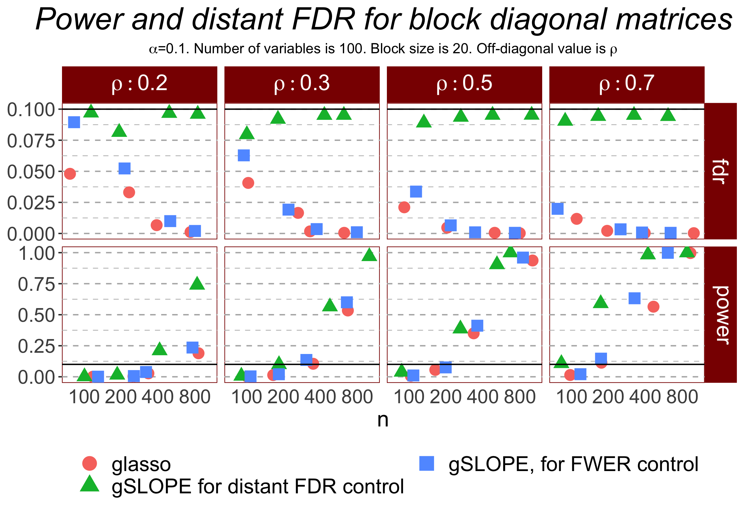
Figure 3: Distant FDR Control. The Figure shows the Distant False Discovery Rate (FDR) control for the block diagonal correlation matrix at a given level $\alpha=0.1$ and when considering $n=100,200,400,800$.

2.3 Alternating Direction Method of Multipliers for Gslope

The solution to (7) can be found using the general alternative direction method of multipliers (ADMM), which has been successfully applied to solve the Glasso optimization problem (see e.g., Scheinberg et al. (2010); Boyd et al. (2011)). The general formulation of ADMM algorithm can be found in Appendix A.

To derive our algorithm, we first note that the optimization problem in (7) is strictly concave. We then derive the corresponding strictly convex and constrained version as follows:

$$\begin{cases}\min_{\boldsymbol{\Theta}}&-\log\det\boldsymbol{\Theta}+\operatorname{tr}\left(\boldsymbol{\Theta}\boldsymbol{S}\right)+J_{\boldsymbol{\lambda}}\left(\boldsymbol{\Theta}\right)\\ s.t.&\boldsymbol{\Theta}>\textbf{0}\;\;.\end{cases},$$ (13)

We can rewrite the problem in (13) as:

$$\begin{cases}\min_{\boldsymbol{\Theta}}&-\log\det\boldsymbol{\Theta}+\operatorname{tr}\left(\boldsymbol{\Theta}\boldsymbol{S}\right)+\mathbb{I}[\boldsymbol{\Theta}>\boldsymbol{0}]+J_{\boldsymbol{\lambda}}\left(\boldsymbol{Y}\right)\\ s.t.&\boldsymbol{\Theta}=\boldsymbol{Y}\end{cases},$$ (14)

where the indicator function $\mathbb{I}[A]=0$ if $A$ holds $\mathbb{I}[A]=\infty$ if $A$ does not hold effectively reduces the domain to the positive-definite matrices.

Furthermore, the augmented Lagrangian function in the inner product form of the problem in (14) is expressed as:

$$\mathcal{L}^{+}(\boldsymbol{\Theta},\boldsymbol{Y},\boldsymbol{Z}) = -\log\det\boldsymbol{\Theta}+\operatorname{tr}\left(\boldsymbol{\Theta}\boldsymbol{S}\right)+\mathbb{I}[\boldsymbol{\Theta}>\boldsymbol{0}]+J_{\boldsymbol{\lambda}}\left(\boldsymbol{Y}\right)$$

$$+\rho\left\langle\boldsymbol{Z},\boldsymbol{\Theta}-\boldsymbol{Y}\right\rangle_{F}+\frac{\rho}{2}\left\|\boldsymbol{\Theta}-\boldsymbol{Y}\right\|_{F}^{2},$$

where $\boldsymbol{Z}$ is the second dual variable, $\rho>0$ is the augmented Lagrangian penalty parameter, $\left\langle\cdot,\cdot\right\rangle_{F}$ is the Frobenius inner product and $\left\|\cdot\right\|_{F}$ is the Frobenius norm inducted by the inner product.

Following the ADMM algorithm described in Appendix A, we minimize the augmented Lagrangian as a function of $\boldsymbol{\Theta}$ and $\boldsymbol{Y}$, implementing the dual update. As for the $(k+1)$-th update of $\boldsymbol{\Theta}$, we obtain:

$$\boldsymbol{\Theta}_{(k+1)}=\arg\min_{\boldsymbol{\Theta}>\textbf{0}}\left\{-\log\det\boldsymbol{\Theta}+\frac{\rho}{2}\left\|\boldsymbol{\Theta}+(\boldsymbol{Z}_{(k)}-\boldsymbol{Y}_{(k)}+\rho^{-1}\boldsymbol{S})\right\|_{F}^{2}\right\}.$$ (16)

After defining the quantity $\boldsymbol{\tilde{S}}_{(k)}=-\boldsymbol{Z}_{(k)}+\boldsymbol{Y}_{(k)}-\rho^{-1}\boldsymbol{S}$, the optimization problem in (16) can be rewritten as:

$$\boldsymbol{\Theta}_{(k+1)}=\arg\min_{\boldsymbol{\Theta}\geq\textbf{0}}\left\{-\log\det\boldsymbol{\Theta}+\frac{\rho}{2}\left\|\boldsymbol{\Theta}-\boldsymbol{\tilde{S}}_{(k)}\right\|_{F}^{2}\right\}.$$ (17)

The gradient of the augmented Lagrangian in (17) is equal to:

$$\nabla_{\boldsymbol{\Theta}}\mathcal{L}^{+}(\boldsymbol{\Theta},\boldsymbol{Y}_{(k)},\boldsymbol{Z}_{(k)})=-\boldsymbol{\Theta}^{-1}+\rho\boldsymbol{\Theta}-\rho\boldsymbol{\tilde{S}}_{(k)}$$ (18)

and, given the convexity of the augmented Lagrangian in (18), for some optimal matrix $\boldsymbol{\Theta}^{*}>\boldsymbol{0}$, we have: $\nabla_{\boldsymbol{\Theta}}\mathcal{L}^{+}(\boldsymbol{\Theta}^{*},\boldsymbol{Y}_{(k)},\boldsymbol{Z}_{(k)})=\boldsymbol{0}$, so that:

$$-(\boldsymbol{\Theta}^{*})^{-1}+\rho\boldsymbol{\Theta}^{*}-\rho\boldsymbol{\tilde{S}}_{(k)}=\boldsymbol{0}.$$ (19)

This means that $\boldsymbol{\Theta}^{*}$ is the solution for the update of $\boldsymbol{\Theta}$. We need to find a positive definite solution $\boldsymbol{\Theta}^{*}$ to guarantee the invertibility of the precision matrix. We start from the spectral decomposition of $\boldsymbol{\tilde{S}}_{(k)}$, defined as $\boldsymbol{\tilde{S}}_{(k)}=\boldsymbol{Q}\boldsymbol{H}\boldsymbol{Q}^{\prime}$, where $\boldsymbol{H}=\operatorname{diag}\{h_{i}\}$. Suppose that there exists a solution of the following type: $\boldsymbol{\Theta}^{*}=\boldsymbol{Q}\boldsymbol{D}\boldsymbol{Q}^{\prime}$, where $\boldsymbol{D}=\operatorname{diag}\{d_{i}\}$ and $d_{i}>0$. Building on these decompositions, we can reformulate the optimal conditions in (19) as $\boldsymbol{Q}(-\boldsymbol{D}^{-1}+\rho\boldsymbol{D}-\rho\boldsymbol{H})\boldsymbol{Q}^{\prime}=\boldsymbol{0}$, which is equivalent to solve the following equality:

$$-\boldsymbol{D}^{-1}+\rho\boldsymbol{D}-\rho\boldsymbol{H}=\boldsymbol{0}.$$ (20)

Moreover, given that both $\boldsymbol{D}$ and $\boldsymbol{H}$ are diagonal matrices, Equation (20) can be expressed as $-d_{i}^{-1}+\rho d_{i}-\rho h_{i}=0\;\forall i$, from which we obtain $d_{i}^{2}-d_{i}h_{i}-\frac{1}{\rho}=0$, which leads to the following solution:

$$d_{i}=\frac{1}{2}\cdot\left\{h_{i}+\sqrt{h_{i}^{2}+\frac{4}{\rho}}\right\}.$$ (21)

We stress the fact that all diagonal elements are positive, given that $\rho>0$. Moreover, $d_{i}>0$ even if $h_{i}\leq 0$. As a result, the condition that $\boldsymbol{\tilde{S}}_{(k)}$ has positive eigenvalues is not required. Therefore, $\boldsymbol{\Theta}^{*}=\boldsymbol{Q}\boldsymbol{D}\boldsymbol{Q}^{\prime}$ is the solution to our problem, where $\boldsymbol{D}=1/2\cdot\operatorname{diag}\left\{h_{i}+\sqrt{h_{i}^{2}+\frac{4}{\rho}}\right\}$. Since the solution depends on the eigenvalues of $\boldsymbol{\tilde{S}}_{(k)}$, the update rule for $\boldsymbol{\Theta}_{(k+1)}$ can be defined as follows:

$$\boldsymbol{\Theta}_{(k+1)}=\mathcal{F}_{\rho}\left(\boldsymbol{\tilde{S}}_{(k)}\right)=\mathcal{F}_{\rho}\left(-\boldsymbol{Z}_{(k)}+\boldsymbol{Y}_{(k)}-\frac{1}{\rho}\boldsymbol{S}\right),$$ (22)

where $\mathcal{F}_{\rho}\left(\boldsymbol{\tilde{S}}_{(k)}\right)\equiv\boldsymbol{Q}\boldsymbol{D}\boldsymbol{Q}^{\prime}$.

As for the update rule of $\boldsymbol{Y}_{(k+1)}$, we obtain the following result:

$$\boldsymbol{Y}_{(k+1)}= \arg\min_{\boldsymbol{Y}} \mathcal{L}^{+}\left(\boldsymbol{\Theta}_{(k+1)},\boldsymbol{Y},\boldsymbol{Z}_{(k)}\right)$$

$$= \arg\min_{\boldsymbol{Y}} -\log\det\boldsymbol{\Theta}_{(k+1)}+\operatorname{tr}\left(\boldsymbol{\Theta}_{(k+1)}\boldsymbol{S}\right)+J_{\boldsymbol{\lambda}}\left(\boldsymbol{Y}\right)+\rho\left\langle\boldsymbol{Z}_{(k)},\boldsymbol{\Theta}_{(k+1)}-\boldsymbol{Y}\right\rangle_{F}$$

$$+\frac{\rho}{2}\left\|\boldsymbol{\Theta}_{(k+1)}-\boldsymbol{Y}\right\|_{F}^{2}$$

$$= \arg\min_{\boldsymbol{Y}} J_{\boldsymbol{\lambda}}\left(\boldsymbol{Y}\right)+\frac{\rho}{2}\left\|\boldsymbol{Y}-(\boldsymbol{\Theta}_{(k+1)}+\boldsymbol{Z}_{(k)})\right\|_{F}^{2}=\mathrm{prox}_{(J_{\lambda},\rho)}(\boldsymbol{\Theta}_{(k+1)}+\boldsymbol{Z}_{(k)}),$$ (23)

where

$$\mathrm{prox}_{(J_{\lambda},\rho)}(t)=\arg\min_{x}J_{\lambda}(x)+\frac{\rho}{2}||t-x||_{F}^{2}$$

is the proximal operator of the SLOPE norm. An efficient algorithm for solving this proximal optimization problem is provided e.g. in Bogdan et al. (2015).

Building on the results derived above, we report below the ADMM algorithm that we developed for solving the Gslope problem.

$\boldsymbol{Y}_{(0)}\leftarrow\boldsymbol{\tilde{Y}}$, $\boldsymbol{Z}_{(0)}\leftarrow\boldsymbol{\tilde{Z}}$, $\rho\leftarrow\rho_{(0)}>0$, $k\leftarrow 1$;

while convergence criterion is not satisfied do

      Perform the spectral decomposition of the $\boldsymbol{\tilde{S}}_{(k)}$ matrix: $\boldsymbol{\tilde{S}}_{(k)}=\boldsymbol{Q}\boldsymbol{H}\boldsymbol{Q}^{\prime}$;

       $\boldsymbol{\Theta}_{(k+1)}\coloneqq\mathcal{F}_{\rho}(\boldsymbol{\tilde{S}}_{(k)})$;

       $\boldsymbol{Y}_{(k+1)}\coloneqq\mathrm{prox}_{(J_{\lambda},\rho)}(\boldsymbol{\Theta}_{(k+1)}+\boldsymbol{Z}_{(k)})$;

       $\boldsymbol{Z}_{(k+1)}\coloneqq\boldsymbol{Z}_{(k)}+\rho(\boldsymbol{\Theta}_{(k+1)}-\boldsymbol{Y}_{(k+1)})$;

       $k\leftarrow k+1$;

end while

Algorithm 1 Alternating Direction Method of Multipliers for Gslope

Theorem 5.

Algorithm (1) produces a sequence of precision matrices which converges to the optimal solution in the objective function value.

Proof.

• Firstly, notice that both functions that are part of the objective function, $-\log\det\boldsymbol{\Theta}+\operatorname{tr}\left(\boldsymbol{\Theta}\boldsymbol{S}\right)+\mathbb{I}[\boldsymbol{\Theta}>\boldsymbol{0}]$ and $J_{\boldsymbol{\lambda}}\left(\boldsymbol{\Theta}\right)$, are closed and proper convex functions.

• Secondly, by the Saddle Point Theorem (see (Boyd and Vandenberghe, 2004)), the unaugmented Lagrangian of the Gslope has a saddle point.

Thus, the assumptions for the convergence of the ADMM algorithm from (Boyd et al., 2011) are met, which concludes our proof.

3 Dealing with $t$-distributed data

The methods discussed so far rely on the assumption that $\boldsymbol{X}$ follows a multivariate normal distribution. However, there exist contexts in which this assumption is restrictive. Therefore, the accuracy of the resulting estimates and inference may be undermined by potential deviations from Gaussianity. For instance, the impact of false-positive edges in Glasso-estimated graphs significantly increases in the presence of heavy-tailed distributions (Cribben, 2019). This limitation has prompted the development of alternative methods. Among them, the Tlasso method introduced by Finegold and Drton (2011) has proven to be an effective tool for a robust graphical inference in presence of outliers or contaminated data (Finegold and Drton, 2014; Torri et al., 2018; Cribben, 2019; Torri et al., 2019). In this section, we extend the method introduced by Finegold and Drton (2011) with a new Tslope algorithm, which exploits the advantages of the SL1 penalty described in Section 2.

In contrast to Section 2, we now assume that $\boldsymbol{X}$ follows a multivariate $t$-distribution with $\nu>2$ degrees of freedom; that is, $\boldsymbol{X}\sim t_{p}\left(\boldsymbol{\mu},\boldsymbol{\Psi},\nu\right)$, where $\boldsymbol{\mu}=\mathbb{E}\left[\boldsymbol{X}\right]\in\mathbb{R}^{p}$ is the expected value vector of $\boldsymbol{X}$, whereas $\boldsymbol{\Psi}$ is the $p\times p$ positive definite dispersion matrix. Under the assumption $\boldsymbol{X}\sim t_{p}\left(\boldsymbol{\mu},\boldsymbol{\Psi},\nu\right)$, the density function of $\boldsymbol{X}$ is defined as follows:

$$f_{\boldsymbol{X}}\left(x\mid\boldsymbol{\mu},\boldsymbol{\Psi},\nu\right)=\frac{\Gamma[(\nu+p)/2]}{(\pi\nu)^{\frac{p}{2}}\Gamma(\nu/2)\left(\det\boldsymbol{\Psi}\right)^{\frac{1}{2}}}\left[1+\frac{1}{\nu}\left(\mathbf{x}-\boldsymbol{\mu}\right)^{\prime}\boldsymbol{\Psi}^{-1}\left(\mathbf{x}-\boldsymbol{\mu}\right)\right]^{-\frac{\nu+p}{2}},$$ (24)

where $\Gamma(\cdot)$ denotes the gamma function,

Given $n$ realizations of the random vector $\boldsymbol{X}\sim t_{p}\left(\boldsymbol{\mu},\boldsymbol{\Psi},\nu\right)$, denoted as $\mathbf{x}^{(1)},\ldots,\mathbf{x}^{(n)}$, the log-likelihood of the data takes the following form:

$$\mathcal{L}\left(\boldsymbol{\mu},\boldsymbol{\Psi},\nu\right) = \log\prod_{j=1}^{n}f_{\boldsymbol{X}}\left(\mathbf{x}^{(j)}\mid\boldsymbol{\mu},\boldsymbol{\Psi},\nu\right)$$

$$= -n\log\Gamma\left(\frac{\nu}{2}\right)+n\log\Gamma\left(\frac{\nu+p}{2}\right)-\frac{np}{2}\log\nu-\frac{np}{2}\log\pi$$

$$- \frac{n}{2}\log\det\boldsymbol{\Psi}^{-1}-\left(\frac{\nu+p}{2}\right)\sum_{j=1}^{n}\log\left[\nu+\delta_{\mathbf{x}^{(j)}}\left(\boldsymbol{\mu},\boldsymbol{\Psi}\right)\right],$$ (26)

where $\delta_{\mathbf{x}^{(j)}}\left(\boldsymbol{\mu},\boldsymbol{\Psi}\right)=\left(\mathbf{x}^{(j)}-\boldsymbol{\mu}\right)^{\prime}\boldsymbol{\Psi}^{-1}\left(\mathbf{x}^{(j)}-\boldsymbol{\mu}\right)$ is the the Mahalanobis distance.

It is important to highlight the fact that the covariance matrix of $\boldsymbol{X}$ (i.e. $\boldsymbol{\Sigma}$) can be expressed as a function of $\boldsymbol{\Psi}$, through the following relationship: $\boldsymbol{\Sigma}=\frac{\nu}{\nu-2}\boldsymbol{\Psi}$. Following Finegold and Drton (2011), for notational convenience, we define the precision matrix of a multivariate $t$-distribution as $\boldsymbol{\Theta}=\boldsymbol{\Psi}^{-1}$, so that we have a clear connection with the Gaussian graphical model described in Sections 1 and 2. Similar to the Glasso and Gslope methods (see Sections 1 and 2), we aim at estimating networks in which vertices $i$ and $j$ are not connected by an edge if $\theta_{i,j}=0$. We still employ a penalty function to promote sparsity in the precision matrix. Nevertheless, in contrast to the Gaussian framework, the condition $\theta_{i,j}=0$ no longer implies conditional independence when using the $t$-distribution (Baba et al., 2004). However, despite the lack of conditional independence, the $t$-distribution provides the following property: if two vertices $i$ and $j$ are separated by a set of nodes $\mathtt{C}$ in $\mathtt{G}$, then $X_{i}$ and $X_{j}$ are conditionally uncorrelated given $X_{\mathtt{C}}$ (Finegold and Drton, 2011). Therefore, it is reasonable to replace conditional independence with zero partial correlation or zero conditional correlation. By doing so, disconnected nodes in a given graph can be considered orthogonal to each other after the effects of other vertices of the same network are removed (Torri et al., 2018).

When assuming $\boldsymbol{X}\sim t_{p}\left(\boldsymbol{\mu},\boldsymbol{\Psi},\nu\right)$, the lack of density factorization properties with $t$-distributions complicates the likelihood inference (Finegold and Drton, 2011). However, we can efficiently estimate the parameters of interest by implementing the Expectation-Maximization (EM) algorithm proposed by Finegold and Drton (2011), that we adapt to our Tslope specification. In particular, the EM algorithm builds on the scale-mixture representation of the $t$-distribution (Finegold and Drton, 2011) described below, which leads to relevant computational advantages. Specifically, let $\boldsymbol{W}\sim\mathcal{N}_{p}(\boldsymbol{0},\boldsymbol{\Psi})$ be a multivariate normal random vector independent of the Gamma random variable $\tau\sim\Gamma(\nu/2,\nu/2)$, then:

$$\boldsymbol{X}=\boldsymbol{\mu}+\frac{\boldsymbol{W}}{\sqrt{\tau}}\sim t_{p}(\boldsymbol{\mu},\boldsymbol{\Psi},\nu).$$ (27)

This scale-mixture representation allows for easy sampling and emphasizes the fact that the $t$-distribution leads to more robust inference, as extreme observations can be the result of small $\tau$ values (Finegold and Drton, 2011). Moreover, it allows us to derive the conditional distribution of $\tau$ given $\boldsymbol{X}$ and $\nu$ :

$$f_{\tau}\left(\tau\mid\boldsymbol{X}\right)\sim\Gamma\left(\frac{\nu+p}{2},\frac{\nu+\left(\boldsymbol{X}-\boldsymbol{\mu}\right)^{\prime}\boldsymbol{\Psi}^{-1}\left(\boldsymbol{X}-\boldsymbol{\mu}\right)}{2}\right).$$ (28)

Equation (28) immediately implies that conditional on $\tau$ :

$$f_{\boldsymbol{X}}\left(\mathbf{x}\mid\tau\right)\sim\mathcal{N}_{p}\left(\boldsymbol{\mu},\boldsymbol{\Psi}/\tau\right).$$ (29)

Now, suppose that we observe the following sequence of the hidden Gamma-random variables:

$$\tau^{(1)},...,\tau^{(n)}\sim\Gamma(\nu/2,\nu/2).$$ (30)

Equations (29) and (30) form a scale-mixture model with the following T-slope penalized complete log-likelihood function (Liu, 1997):

$$\mathcal{L}\left(\boldsymbol{\mu},\boldsymbol{\Theta}\mid\mathbf{x},\boldsymbol{\tau},\nu\right)\propto-\frac{1}{2}\sum_{j=1}^{n}\tau^{(j)}\left(\mathbf{x}^{(j)}-\boldsymbol{\mu}\right)^{\prime}\boldsymbol{\Theta}\left(\mathbf{x}^{(j)}-\boldsymbol{\mu}\right)+\frac{n}{2}\log\det\boldsymbol{\Theta}-J_{\boldsymbol{\lambda}}\left(\boldsymbol{\Theta}\right)\;\;,$$

where, $\mathbf{x}=(x^{(1)},\ldots,x^{(n)})$, $\boldsymbol{\tau}=(\tau^{(1)},\ldots,\tau^{(n)})$, and the symbol $\propto$ indicates that irrelevant additive constants are omitted.

Following Finegold and Drton (2011), we employ the EM algorithm that we adapt to our Tslope method. This algorithm is described below:

• E-step: we compute the conditional expectation of the penalized complete log-likelihood function given the realization $\mathbf{x}^{(j)}$. Since the penalized log-likelihood is a linear function of $\tau$, we only need to compute the conditional expectations of the coordinates of $\tau$, which are equal to:

  $$\mathbb{E}\left[\tau^{(j)}\mid\mathbf{x}^{(j)}\right]=\frac{\nu+p}{\nu+\left[\delta_{\mathbf{x}^{(j)}}\left(\boldsymbol{\mu},\boldsymbol{\Psi}\right)\right]}.$$ (31)

  Given the current estimates of $\boldsymbol{\mu}$ and $\boldsymbol{\Psi}^{-1}$, denoted, respectively, as $\widehat{\boldsymbol{\mu}}_{(k)}$ and $\widehat{\boldsymbol{\Psi}}^{-1}_{(k)}$, we can compute $\hat{\tau}_{(k+1)}^{(j)}$ at the $(k+1)$-th iteration as:

  $$\hat{\tau}_{(k+1)}^{(j)}=\frac{\nu+p}{\nu+\left[\delta_{\mathbf{x}^{(j)}}\left(\widehat{\boldsymbol{\mu}}_{(k)},\widehat{\boldsymbol{\Psi}}^{-1}_{(k)}\right)\right]},\quad j=1,...,n.$$ (32)

• M-step: we maximize the complete log-likelihood to obtain the parameter estimates at iteration $k+1$:

  $$\widehat{\boldsymbol{\mu}}_{(k+1)}=\frac{\sum_{j=1}^{n}\hat{\tau}_{(k+1)}^{(j)}\mathbf{x}^{(j)}}{\sum_{j=1}^{n}\hat{\tau}_{(k+1)}^{(j)}}$$ (33)

  $$\boldsymbol{S}_{(k+1)}=\frac{1}{n}\sum_{j=1}^{n}\hat{\tau}_{(k+1)}^{(j)}\left(\mathbf{x}^{(j)}-\widehat{\boldsymbol{\mu}}_{(k+1)}\right)\left(\mathbf{x}^{(j)}-\widehat{\boldsymbol{\mu}}_{(k+1)}\right)^{\prime}.$$ (34)

  We implement the Gslope method (see Section 2) to obtain the estimate of the precision matrix $\boldsymbol{\Psi}_{(k+1)}^{-1}\equiv\boldsymbol{\Theta}_{(k+1)}$. We remind the reader that the Gslope method solves the following optimization problem: $\widehat{\boldsymbol{\Theta}}_{(k+1)}=\arg\max_{\boldsymbol{\Theta}}\left\{\log\det\boldsymbol{\Theta}-\operatorname{tr}\left(\boldsymbol{\Theta}\boldsymbol{S}_{(k+1)}\right)-J_{\boldsymbol{\lambda}}(\boldsymbol{\Theta})\right\}$ , where $J_{\boldsymbol{\lambda}}(\boldsymbol{\Theta})$ is the SL1 penalty defined in Equation (6).

We iterate the E- and M-steps until we satisfy the following convergence criterion: $\left\|\widehat{\boldsymbol{\Theta}}_{(k+1)}-\widehat{\boldsymbol{\Theta}}_{(k)}\right\|<\epsilon$, where $\epsilon$ is a sufficiently small threshold.

4 Simulation study

In this section we report the results of the simulation study comparing Gslope and Tslope to other state-of-art methods for the estimation of the precision matrix.

4.1 Simulation set-up

For our simulation study, we rely on the R package huge, which allows to simulate data for undirected graphical models for many different network configurations, including cluster, random, hub, scale-free and band structures. Having specified the desired network structure, the number of nodes $p$ and the so called Magnitude Ratio (MR), the package returns an oracle covariance matrix $\boldsymbol{\Sigma}$ and an oracle precision matrix, $\boldsymbol{\Theta}$. The oracle covariance matrix $\boldsymbol{\Sigma}$ is then used as an input to a data generating process, from which $n$ data points are sampled. These data are then used to estimate the oracle covariance matrix using the considered methods of estimation of sparse graphical models.
Here, we resort to presenting the results for the cluster and the random networks, as we believe that those networks capture the majority of real world applications. For example, different stocks can be grouped according to different economic sectors. Still, their relationships are far from perfect and random linkages across such sectors are often observed.
To set the Magnitude Ratio (MR), which is given as $MR=\frac{u+v}{v}$, we need to choose a value for $u$, which is the value that is added to the diagonal elements of the precision matrix after it has been transformed to a positive semi-definite matrix, and $v$ that represent the off-diagonal non-zero entries of the precision matrix. The off-diagonal entries are modified to ensure the invertibility of the covariance matrix. As such, the magnitude ratio regulates the dominance of the diagonal entries, as compared to the off-diagonal entries. If the MR is close to zero, the off-diagonal entries are dominated by the diagonal entries. On the other hand, if MR is large, then the off-diagonal elements dominate. In what follows, we choose MR=0 and MR=1.43 to capture different relationships between the main diagonal and off-diagonal elements. Figure 4 shows the heatmaps of the partial correlation structure of the considered networks. The figure illustrates how a higher magnitude ratio increases the dominance of the off-diagonal elements.
Finally, given a sample of $n$ independent $p$-dimensional data vectors, we aim to estimate $\boldsymbol{\Theta}$ directly, using our newly introduced Gslope and Tslope algorithm, and further compare its performance to other state-of-the-art methods for estimation the precision matrix, including the inverse of the sample covariance matrix (Sample, only when $n>p$), graphical elastic net (Elastic Net, Kovács et al. (2021); Bernardini et al. (2021)), the Resampling Of Penalized Estimates (ROPE, Kallus et al. (2017)), the Glasso (Glasso, Friedman et al. (2008)), and the Tlasso (Tlasso, Finegold and Drton (2011)).

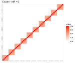
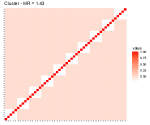
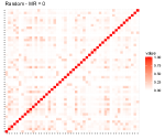
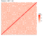
(a) (b) (c) (d)

Figure 4: Heatmaps of the partial correlation matrices for cluster networks ((a) and (b)) and the random network structures ((c) and (d)) and the magnitude ratios $MR=0$ and $MR=1.43$.

To analyse the robustness of our new methods with regard to the data generating processes, we make the following three assumptions for each of the underlying distributions:

1. Multivariate Gaussian distribution: $\boldsymbol{X}\sim N_{p}(0,\boldsymbol{\Sigma})$

2. Multivariate t-student distribution: $\boldsymbol{X}\sim t_{p}(0,\boldsymbol{\Sigma},\nu)$, with $\nu=4$

3. Multivariate Mixture distribution: $\boldsymbol{X}\sim 0.5\times N_{p}(0,\boldsymbol{\Sigma})+0.5\times t_{p}(0,\boldsymbol{\Sigma},\nu)$, with $\nu=4$

Given, that we want to compare all methods in situations where both $n>p$ and $n<p$, we fix the number of nodes to be $p=100$, and let the number of observations vary, drawing first $n=250$ and then $n=50$ data points. With the two network configurations (i.e. cluster and random), the two different values of MR (i.e. MR=0 and MR=1.43) and the three different distributional assumptions (i.e. Gaussian, t-student and mixed), we consider a total of 24 distinct simulation set-ups.

4.2 Tuning parameter set-up

All methods - except the sample estimate - depend on a single tuning parameter or a decreasing sequence of tuning parameters, which trade off model complexity and sparsity.

For Glasso and Tlasso we choose $\lambda$ according to the formula (8) of Banerjee et al. (2008), with $\alpha=0.05$ for $n=250$ and $\alpha=0.4$ for $n=50$. This goes along the statistical practice of using larger significance levels for smaller sample sizes, which allows to enhance estimation properties by preserving a high power of detection of important edges and reducing the bias due to the $L_{1}$ norm shrinkage.

In case of Gslope and Tslope we resort to the Benjamini-Hochberg (BH) sequence of the tuning paramaters (12). As illustrated in Section 2, this sequence allows Gslope to control the distant FDR when the data come from the multivariate normal distribution. Figure 5 illustrates that the same sequence allows Tslope to control the distant FDR when the data come from the multivariate t-distribution and $n>p$. For consistency with Glasso, in the remaining part of this section we will set the $\alpha$ parameters for Gslope and Tslope at $\alpha=0.05$ for $n=250$ and $\alpha=0.4$ for $n=50$. As the sequence of tuning parameters for Gslope and Tslope is decaying we expect the overall shrinkage magnitude to be larger for Glasso and Tlasso, as compared to the Slope procedures. Thus, we expect Slope methods to produce denser graphs.

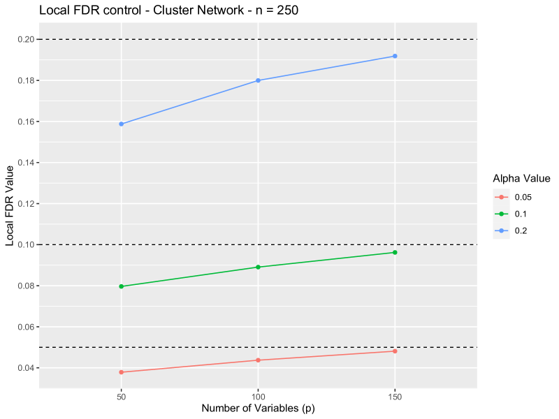
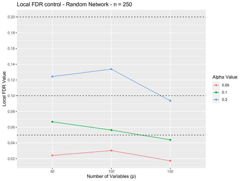
Figure 5: The distant False Discovery Rate (FDR) control by Tslope for the data generated according to the multivariate t-distribution and the cluster and random network with $MR=0$. Here $alpha=0.05,0.1,0.2$, $n=250$ and $p=50,100,150$, respectively.

ROPE and Elastic Net require the selection of the tuning parameter for the Lasso part of the algorithm. In our simulations we fixed this parameter at the same value as for Glasso, i.e. according to the formula (8). We also verified that the performance of these procedures is not substantially different when the selection of this tuning parameter is performed using cross-validation. Furthermore, for Elastic Net we set the value of the mixing parameter ($\alpha$ in glmnet) to 0.5 and for ROPE we used the default value of the FDR nominal level $q=0.1$.

4.3 Accuracy characteristics

While the tuning sequences for Gslope and Tslope were selected for the distant FDR control, it is interesting to verify how they perform with respect to other important measures of the accuracy of the precision matrix estimation. In our study we consider the two following standard accuracy measures.

• F1 score.

  $$\text{F1-Score}=\frac{\text{True Positives}}{\text{True Positives}+\frac{1}{2}(\text{False Positives}+\text{False Negatives})}\;\;,$$ (35)

  whereas the True Positives are the number of edges which are both in the true and estimated precision matrix, the False positives are those which are active in the estimated precision matrix, but not in the true one, and the False negatives are those edges, which the procedure fails to identify. The F1 statistics is defined on the interval [0,1]. A value of 1 indicates optimal model selection properties, in which only those edges have been selected that are also present in $\boldsymbol{\Theta}$.
  

• Frobenius Norm.

  $$D_{F}(\widehat{\boldsymbol{\Theta}},\boldsymbol{\Theta})=||\widehat{\boldsymbol{\Theta}}-\boldsymbol{\Theta}||=\sqrt{(tr((\widehat{\boldsymbol{\Theta}}-\boldsymbol{\Theta})(\widehat{\boldsymbol{\Theta}}-\boldsymbol{\Theta})^{\prime})}\;\;,$$ (36)

  where a lower value indicates a higher accuracy of the estimated model. Different to the F1-Score, the Frobenius Norm distance allows us to evaluate the magnitude of the estimated edges as compared to the oracle precision matrix.
  

4.4 Simulation results

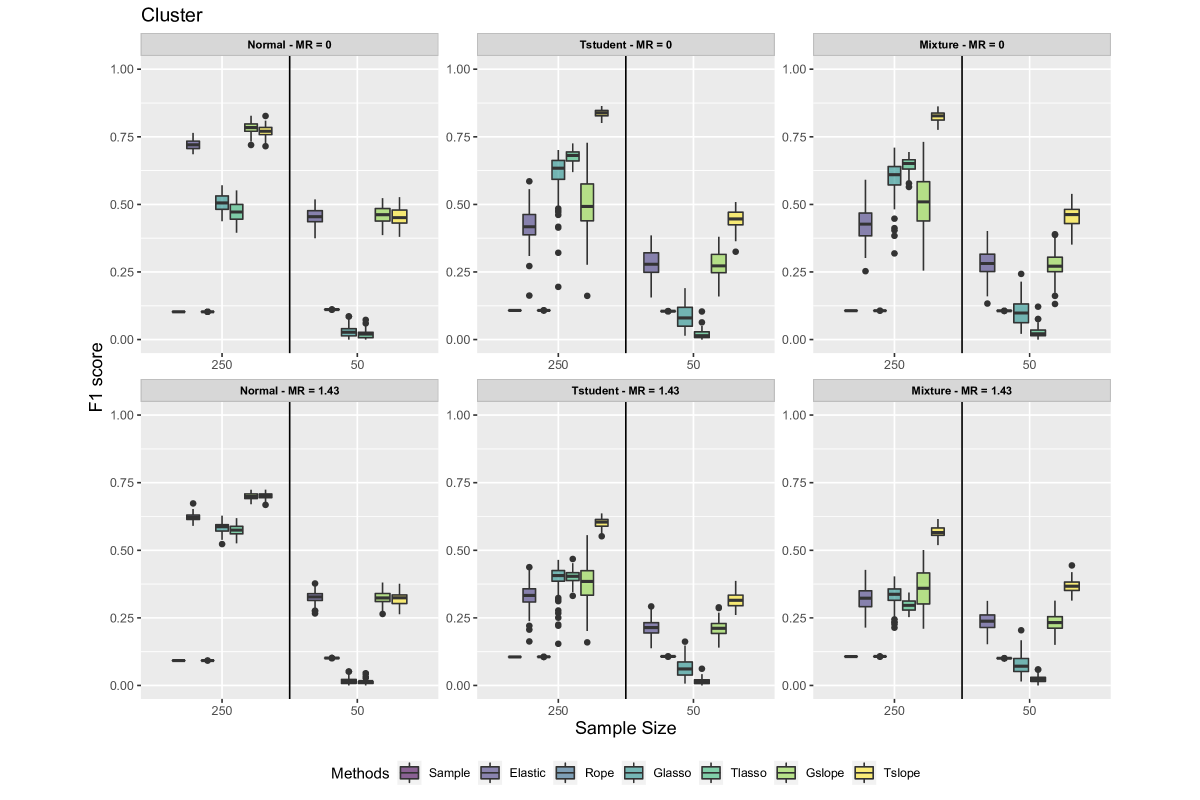
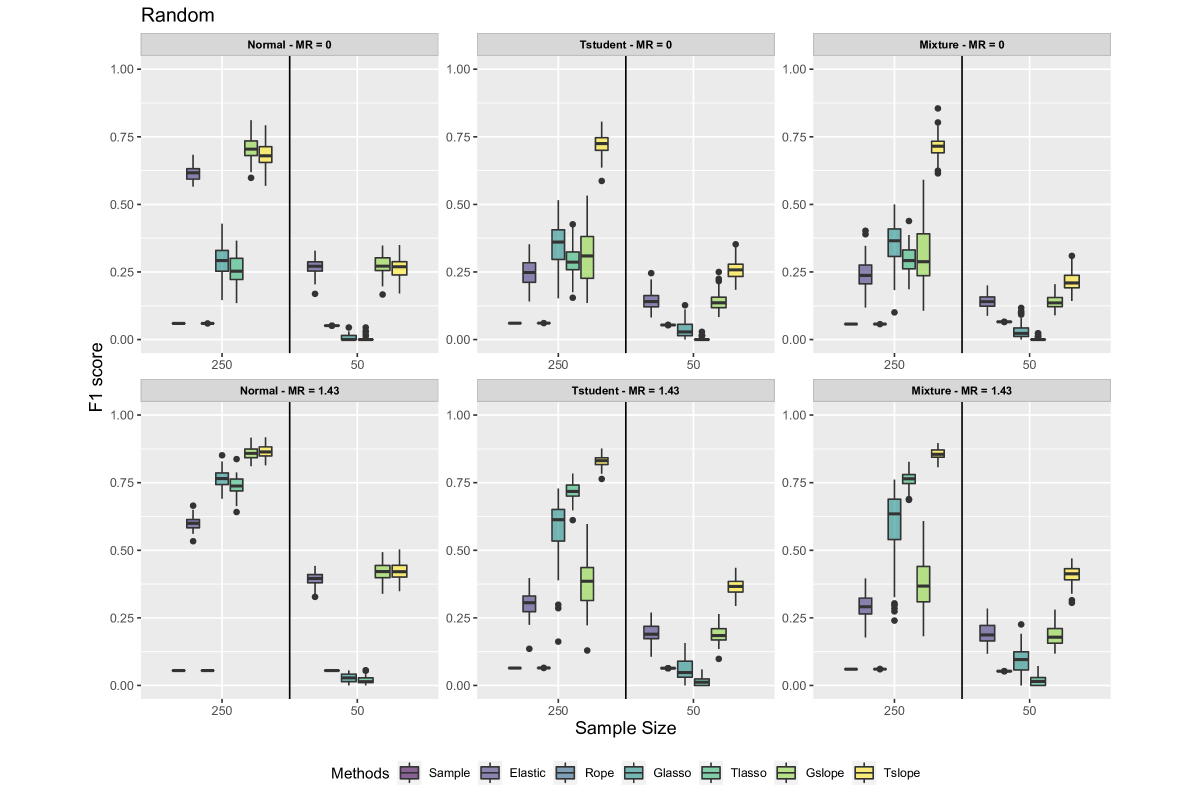
Figure 6: F1- Score Boxplots. The figure shows the F-Measure Boxplots across all 100 simulation runs for the 24 distinct network configurations for both the low dimensional ($n>p$) and the high dimensional setting ($n<p$), respectively.

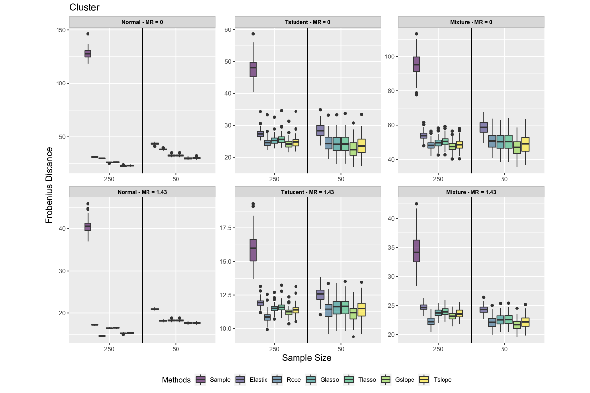
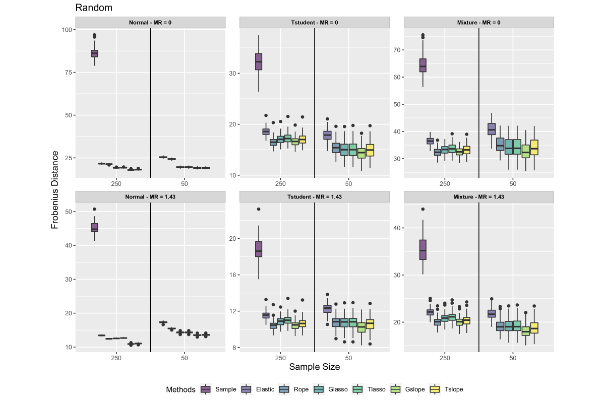
Figure 7: Frobenius Norm Distance Boxplots. The figure shows the Frobenius Norm Boxplots across all 100 simulation runs for the 24 distinct network configurations for both the low dimensional ($n>p$) and the high dimensional setting ($n<p$), respectively.

Figure 6 reports the boxplots of the F1-Score across 100 simulations for both the cluster (top two rows) and the random (bottom two rows) network structure, with MR=0 (1st and 3rd row) and MR=1.43 (2nd and 4th rows), respectively, and considering in each subplot on the left the low dimensional setting with $n>p$ (i.e. $n=250$ and $p=100$), and on the right the high dimensional setting with $n<p$ (i.e. $n=50$ and $p=100$). Boxplots in the first column consider the Gaussian case, in the second column the t-Student and in the 3rd column the Mixture distribution. In each subplot, from left to right, we report the results for the Sample, the Elastic Net, the Rope, the Glasso, the Tlasso, as well as the Gslope and Tslope procedures.
Looking at the results for the low dimensional settings (i.e. $n=250$, $p=100$), both Gslope and Tslope consistently outperform all other methods in the Gaussian case, irrespective of the network configuration and the magnitude ratio. Furthermore, even when considering non-Gaussian distributions, the graphical slope methods perform among the best. Especially, our newly introduced method Tslope shows its adaptivity with respect to the underlying distribution and the presence of fatter tails. While Tslope performs in line with Gslope under the Gaussian setting, it outperforms Gslope for a t-Student and a mixture distribution. This observation is robust to the network configuration, and towards the assumed magnitude ratio.
It is interesting to observe that for this low dimensional setup, both the sample and the Rope methods performs worse than other methods. As both do not impose any sparsity onto the estimated covariance structure, they fail to dissect the underlying graph structure.
Reducing the number of observations, while keeping the number of parameters constant ($n=50<p=100$), Figure 6 shows that all methods suffer in extracting the true underlying covariance structure as compared to the low dimensional case. This is especially true for the Lasso methods, while Elastic Net, Gslope and Tslope perform among the best. In fact, for the cluster network and independent of the magnitude ratio, Gslope and Tslope perform in line with the Elastic Net under the Gaussian assumption, while again Tslope outperforms all methods for non-Gaussian data. These observations also hold for the random network structure.
Finally, it can be observed that the performance of the SLOPE procedures (i.e. Gslope and Tslope) is best when the network structure is characterized by truly distinct groups of features. This is evident from the performance of SLOPE methods in the cluster network structure with a low magnitude ratio and the random network structure with a high magnitude ratio. Reconsidering the heatmaps of Figure 4, we can see that Panel (a) and Panel (d) will form more distinct groups of features, while the networks in Panel (b) and (c) represent a more in-distinctive setting. As the unit ball of the dual SLOPE norm takes a form of a permutahedron, SLOPE has a natural ability to cluster precision (i.e., also partial correlations) parameters into the groups with the same or very similar value (see e.g., Schneider and Tardivel (2019); Skalski et al. (2022); Bogdan et al. (2022)). This feature helps the method to better extract the underlying covariance structure in the environments of Panel (a) and (d).

Concerning the Frobenius distance, Figure 7 confirms our findings from above, showing that Gslope and Tslope represent the best performing methods across all state-of-the-art sparse graphical modelling approaches. There is only one exception for a Gaussian distribution in a cluster network and when MR=1.43. Here, the Rope method performs exceptionally well, but still in line with the Slope procedures.
Comparing among the Gslope and Tslope procedures, Gslope has a marginally better ability to extract the magnitude of the respective edges with a lower variability than Tslope, whereas this observation holds across all of the network configurations and when considering both the low and high dimensional setting. While for Gaussian data, as expected, Gslope performs remarkably well, for non-Gaussian data, Tslope stands out, with a better performance in uncovering the relationships among the parameters and only a marginally neglectable inferior performance to Gslope of estimating the magnitude of those relationships.

5 Empirical analysis

5.1 Gene expression data

Wille et al. (2004) and Kovács et al. (2021) use graphical models to analyze a real-world dataset made of $p=39$ expression levels of isoprenoid genes from $n=118$ samples from the plant Arabidopsis Thaliana. Figure 8 illustrates the results of our analysis of this data set with different graphical methods tested in our simulation study, which show that differences observed in simulations persist also in these real-world data. Firstly, we can observe that Rope and Elastic Net recover very dense graphs, whose structure is rather difficult to analyze. On the other hand Glasso and Tlasso using $\lambda$ selected according to Banerjee et al. (2008) at the FWER level $\alpha=0.05$ provides graphs which seem to be too sparse. Specifically, they leave out several unconnected nodes, which seem to be rather unrealistic in the gene expression data. The Slope methods are placed in the middle, with Gslope identifying a denser graphical model than Tslope. Both methods seem capable of clustering genes that appear to be related (e.g. PPDS1 and PPDS2 or GGPPS2, GGPPS4, GGPPS5, GGPPS8, GGPPS9, GGPPS10) as suggested by Wille et al. (2004). Following the interpretation by Wille et al. (2004) and results from our simulations, it seems that Tslope can better deal with noise in the data and avoids detecting a larger number of false discoveries, as some of the connections identified by Gslope appear hard to be interpreted from a biological perspective. However, by studying the common edge sets and the difference among the estimated graphical models, we can gain a better insights on which relationship might be persistent and which ones might need further investigation as they are always not detected.

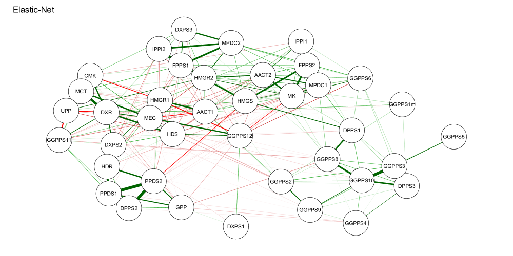
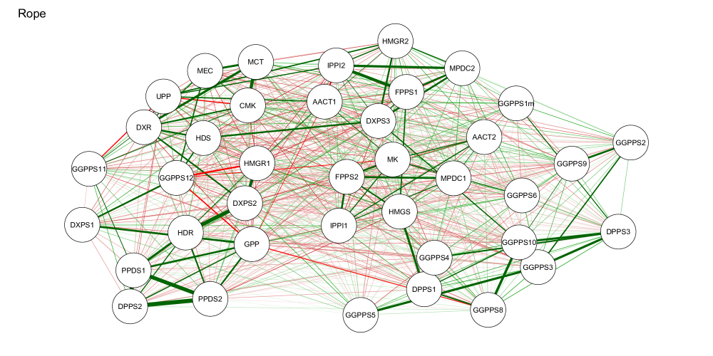
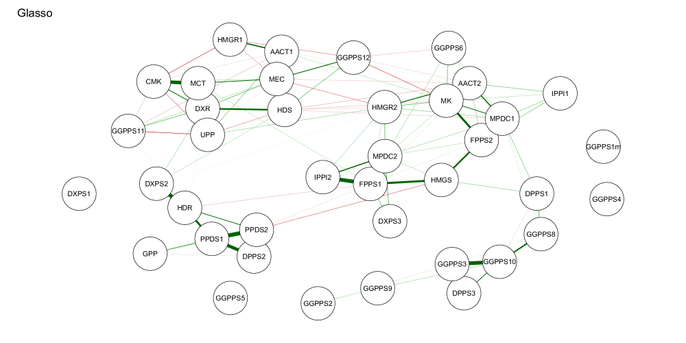
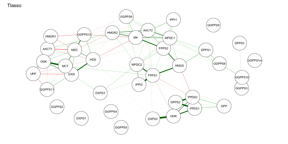
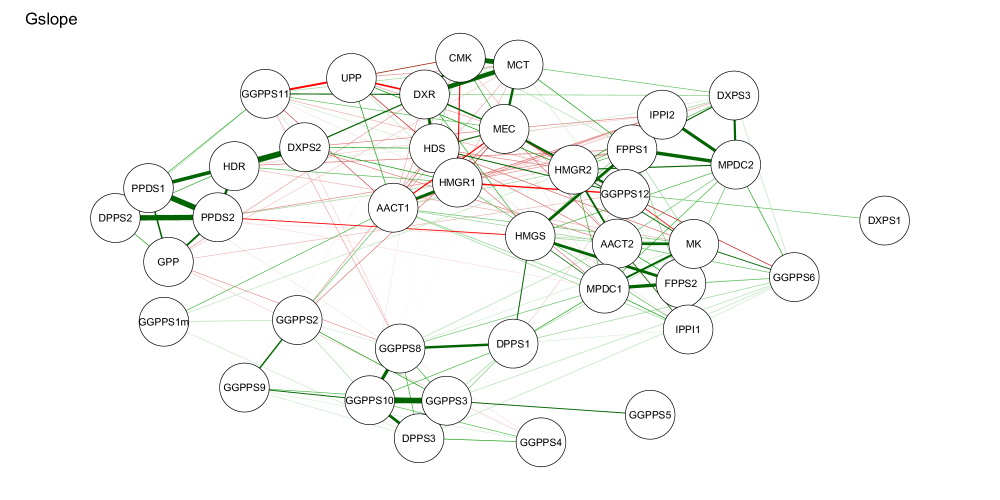
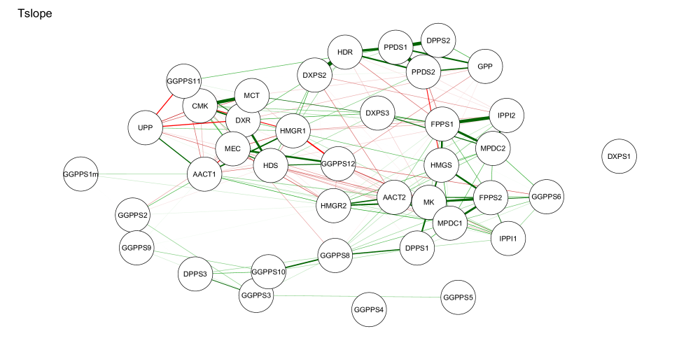
Figure 8: Gene expression networks produced by different methods of graphical model selection.

5.2 Portfolio optimization

In the parallel article Riccobello et al. (2022) Gslope and Tslope were applied for estimating the assets’ precision matrix in the context of portfolio selection. Extensive simulation and real-world analyses highlight the superiority of our new methods over other state-of-the-art approaches, especially with regard to clustering similar assets and stability characteristics in a high-dimensional scenarios. The empirical real data analysis further highlights the improvements in terms of risk and risk-adjusted returns provided by Gslope and Tslope for large portfolios, including assets with heavy-tailed distributions. At the same time, these methods show low turnover rates, bringing further advantages with regard to the impact of transaction costs.

6 Discussion

In this article, we introduced two novel regularization methods for the estimation of high-dimensional precision matrices, with the penalty defined by the Sorted L-One norm (SLOPE, Bogdan et al. (2013, 2015)). First of these methods, Gslope, is designed for estimating gaussian graphical models. The second method, Tslope, extends Gslope to the situation when the distribution of the considered random vector has heavy tails. We proposed and implemented an ADMM algorithm for solving the Gslope optimization problem and an EM algorithm for solving Tslope. We also proposed tuning parameters and tuning sequences for Glasso, Gslope and Tslope, with the goal of eliminating false edges connecting different graph connectivity components. Firstly, we relaxed the tuning parameter for Glasso introduced in Banerjee et al. (2008), so the probability of including such false ’distant’ edges is still controlled at assumed level while the power to identify the true edges slightly increases. In case of Gslope, we further relax the strength of regularization by using the slowly decaying sequence of tuning parameters based on the Holm (1979) and Hochberg (1988) multiple testing procedures. This version of Gslope provably controls the probability of including the false edges between different connectivity components under the standard assumptions of the validity of the Hochberg procedure. We also introduce a quickly decaying sequence based on the Benjamini and Hochberg (1995) multiple testing procedure, which has been empirically shown to control the percentage of false ’distant’ edges among all discovered edges (distant FDR control), both for Gslope and Tslope , and yields much higher power of identifying important edges. Our empirical studies illustrate that the respective versions of Gslope and Tslope outperform other state-of-the-art methods with respect to the accuracy of identifying the graph structure and the precision of the estimation of the concentration matrix, with Tslope outperforming Gslope when the distribution of the considered random vector has heavy tails. Good properties of our methods have been confirmed by the analysis of real biological and financial data.

Concerning the future development, it would be of interest to further investigate theoretical properties of Gslope and Tslope. Specifically, the results included in Kos (2019); Kos and Bogdan (2020) on the False Discovery Rate (FDR) control of the generalized versions of SLOPE suggest the direction for the formal proof of the asymptotic ’distant’ FDR control by Gslope. Moreover, it would be interesting to extend novel results from Bogdan et al. (2022) on the pattern recovery by SLOPE into the context of graphical models. These new results provide the conditions under which SLOPE can properly identify the low dimensional model by eliminating parameters which are equal to zero and by equalizing estimators of parameters, which are equal to each other. As reported in Bogdan et al. (2022), this additional level of dimensionality reduction allows for a substantial improvement of the estimation accuracy with respect to LASSO. The practical advantages of the clustering properties of Gslope and Tslope in the context of portfolio optimization have been reported in Riccobello et al. (2022).

While the theoretical results on the FDR control and the pattern recovery by SLOPE are very encouraging, it must be noted that they hold under rather stringent assumptions. For example, Gslope can control the number of false edges between the distinct connectivity components but it would be rather difficult (or impossible) to construct the sequence of the tuning parameters to control FDR within the connectivity components. Also, the irrepresentability condition for the pattern recovery by SLOPE is rather restrictive (see Bogdan et al. (2022)). However, as discussed in Jiang et al. (2022); Bogdan et al. (2022); Tardivel et al. (2021), the model selection properties of SLOPE can be substantially improved by using its adaptive version or by clustering values of similar SLOPE estimators (thresholded version). Specifically, theoretical and empirical results from Jiang et al. (2022); Bogdan et al. (2022); Tardivel et al. (2021) suggest that these versions of SLOPE can recover the true model under much weaker assumptions than adaptive or thresholded LASSO. Moreover, adaptive Bayesian version of SLOPE (Jiang et al., 2022) allows for increased efficiency by incorporating the prior knowledge on the model structure. In the future it would be of interest to develop appropriate adaptive or thresholded versions of Gslope and Tslope and investigate their properties.

APPENDIX

Appendix A Alternating Direction Method of Multipliers

The Alternating Direction Method of Multipliers (ADMM) represents an effective tool to solve convex optimization problems [Boyd et al., 2011]. The ADMM algorithm has the convergence properties of the method of multipliers. Moreover, it also possesses the decomposability of the dual ascent. It solves problems that can be expressed in the following form:

$$\begin{cases}\min\quad&f_{0}(\boldsymbol{x})+g_{0}(\boldsymbol{y})\\ s.t.\quad&\boldsymbol{A}\boldsymbol{x}+\boldsymbol{B}\boldsymbol{y}=\boldsymbol{c}\end{cases},$$ (37)

where $\boldsymbol{x}\in\mathbb{R}_{n\times 1}$, $\boldsymbol{y}\in\mathbb{R}_{m\times 1}$, $\boldsymbol{A}\in\mathbb{R}_{p\times n}$, $\boldsymbol{B}\in\mathbb{R}_{p\times m}$, $\boldsymbol{c}\in\mathbb{R}_{p\times 1}$.

Our aim is to find the optimal pair of values $(\boldsymbol{x}^{*},\boldsymbol{y}^{*})$ which solves the problem in (37), given the equality constraints. The corresponding augmented Lagrangian function is defined as:

$$\mathcal{L}^{+}(\boldsymbol{x},\boldsymbol{y},\boldsymbol{\lambda})=f_{0}(\boldsymbol{x})+g_{0}(\boldsymbol{y})+\boldsymbol{\lambda}^{\prime}(\boldsymbol{A}\boldsymbol{x}+\boldsymbol{B}\boldsymbol{y}-\boldsymbol{c})+\frac{\rho}{2}\left\|\boldsymbol{A}\boldsymbol{x}+\boldsymbol{B}\boldsymbol{y}-\boldsymbol{c}\right\|_{2}^{2}.$$ (38)

The ADMM algorithm consists of the following iterations:

$$\begin{cases}\boldsymbol{x}_{(k+1)}\coloneqq&\arg\min_{\boldsymbol{x}}\mathcal{L^{+}}\left(\boldsymbol{x},\boldsymbol{y}_{(k)},\boldsymbol{\lambda}_{(k)}\right)\\ \boldsymbol{y}_{(k+1)}\coloneqq&\arg\min_{\boldsymbol{y}}\mathcal{L^{+}}\left(\boldsymbol{x}_{(k+1)},\boldsymbol{y},\boldsymbol{\lambda}_{(k)}\right)\\ \boldsymbol{\lambda}_{(k+1)}\coloneqq&\boldsymbol{\lambda}_{(k)}+\rho\left(\boldsymbol{A}\boldsymbol{x}_{(k+1)}+\boldsymbol{B}\boldsymbol{y}_{(k+1)}-\boldsymbol{c}\right)\end{cases}.$$ (39)

Similar to the method of multipliers, the Lagrange multiplier is updated using the step size equal to the augmented Lagrangian penalty parameter $\rho$. The variables $\boldsymbol{x}$ and $\boldsymbol{y}$ are alternatively updated, and this explains the denomination of the ADMM algorithm.

It is important to highlight the fact that, under the two assumptions: i) functions $f_{0}(\boldsymbol{x})$ and $g_{0}(\boldsymbol{y})$ are closed, proper and convex; and ii) the augmented Lagrangian function $\mathcal{L}^{+}$ with penalty $\rho=0$ has a saddle point, the ADMM iterates satisfy the following properties:

1. Residual convergence: the residual, defined as $(\boldsymbol{A}\boldsymbol{x}+\boldsymbol{B}\boldsymbol{y}-\boldsymbol{c})_{(k)}$, approaches zero as $k\rightarrow\infty$;

2. Objective convergence: $f_{0}(\boldsymbol{x}_{(k)})+g_{0}(\boldsymbol{y}_{(k)})\rightarrow f_{0}(\boldsymbol{x}^{*})+g_{0}(\boldsymbol{y}^{*})$ as $k\rightarrow\infty$. In other words the objective function approaches its optimal value;

3. Dual variable convergence: $\boldsymbol{\lambda}_{(k)}\rightarrow\boldsymbol{\lambda}^{*}$ as $k\rightarrow\infty$, where $\boldsymbol{\lambda}^{*}$ is a dual optimal point.

The following necessary and sufficient conditions are required to solve the problem in (37):

$$\boldsymbol{A}\boldsymbol{x}^{*}+\boldsymbol{B}\boldsymbol{y}^{*}-\boldsymbol{c}=\boldsymbol{0},$$ (40)

$$\begin{cases}\boldsymbol{0}\in&\partial f(\boldsymbol{x}^{*})+\boldsymbol{A}^{\prime}\boldsymbol{\lambda}^{*}\\ \boldsymbol{0}\in&\partial f(\boldsymbol{y}^{*})+\boldsymbol{B}^{\prime}\boldsymbol{\lambda}^{*}\end{cases},$$ (41)

where $\partial$ denotes the sub-differential operator.

Equation (40) is the primal feasibility condition. In contrast, the set of relationships in (41) represents the dual feasibility condition. The augmented Lagrangian function $\mathcal{L^{+}}\left(\boldsymbol{x}_{(k+1)},\boldsymbol{y},\boldsymbol{\lambda}_{(k)}\right)$ is minimized by $\boldsymbol{y}_{(k+1)}$, which leads to the following result:

$$\boldsymbol{0} \in \partial f\left(\boldsymbol{y}_{(k+1)}\right)+\boldsymbol{B}^{\prime}\boldsymbol{\lambda}_{(k)}+\rho\boldsymbol{B}^{\prime}\left(\boldsymbol{A}\boldsymbol{x}_{(k+1)}+\boldsymbol{B}\boldsymbol{y}_{(k+1)}-\boldsymbol{c}\right)$$ (42)

$$= \partial f\left(\boldsymbol{y}_{(k+1)}\right)+\boldsymbol{B}^{\prime}\left[\boldsymbol{\lambda}_{(k)}+\rho\left(\boldsymbol{A}\boldsymbol{x}_{(k+1)}+\boldsymbol{B}\boldsymbol{y}_{(k+1)}-\boldsymbol{c}\right)\right]$$

$$= \partial f\left(\boldsymbol{y}_{(k+1)}\right)+\boldsymbol{B}^{\prime}\boldsymbol{\lambda}_{(k+1)}.$$

This means that, at each iteration, $\boldsymbol{y}_{(k+1)}$ and $\boldsymbol{\lambda}_{(k+1)}$ satisfy the dual feasibility condition $\boldsymbol{0}\in\partial f(\boldsymbol{y}^{*})+\boldsymbol{B}^{\prime}\boldsymbol{\lambda}^{*}$. We need to satisfy the remaining conditions to achieve the optimal solution. Given that $\boldsymbol{x}_{(k+1)}$ minimizes the augmented Lagrangian function $\mathcal{L^{+}}\left(\boldsymbol{x},\boldsymbol{y}_{(k)},\boldsymbol{\lambda}_{(k)}\right)$, by definition, we obtain:

$$\boldsymbol{0} \in \partial f\left(\boldsymbol{x}_{(k+1)}\right)+\boldsymbol{A}^{\prime}\boldsymbol{\lambda}_{(k)}+\rho\boldsymbol{A}^{\prime}\left(\boldsymbol{A}\boldsymbol{x}_{(k+1)}+\boldsymbol{B}\boldsymbol{y}_{(k)}-\boldsymbol{c}\right)$$ (43)

$$= \partial f\left(\boldsymbol{x}_{(k+1)}\right)+\boldsymbol{A}^{\prime}\left[\boldsymbol{\lambda}_{(k)}+\rho\left(\boldsymbol{A}\boldsymbol{x}_{(k+1)}+\boldsymbol{B}\boldsymbol{y}_{(k+1)}-\boldsymbol{c}\right)+\rho\boldsymbol{B}\left(\boldsymbol{y}_{(k)}-\boldsymbol{y}_{(k+1)}\right)\right]$$

$$= \partial f\left(\boldsymbol{x}_{(k+1)}\right)+\boldsymbol{A}^{\prime}\boldsymbol{\lambda}_{(k+1)}+\rho\boldsymbol{A}^{\prime}\boldsymbol{B}\left(\boldsymbol{y}_{(k)}-\boldsymbol{y}_{(k+1)}\right).$$

We can rewrite the relationship in (43) as: $\rho\boldsymbol{A}^{\prime}\boldsymbol{B}\left(\boldsymbol{y}_{(k+1)}-\boldsymbol{y}_{(k)}\right)\in\partial f\left(\boldsymbol{x}_{(k+1)}\right)+\boldsymbol{A}^{\prime}\boldsymbol{\lambda}_{(k+1)}$ and define its left side as: $\boldsymbol{s}_{(k+1)}=\rho\boldsymbol{A}^{\prime}\boldsymbol{B}\left(\boldsymbol{y}_{(k+1)}-\boldsymbol{y}_{(k)}\right)$. This quantity is the dual residual of the dual feasibility condition $\boldsymbol{0}\in\partial f\left(\boldsymbol{x}^{*}\right)+\boldsymbol{A}^{\prime}\boldsymbol{\lambda}^{*}$ at iteration $k+1$. In contrast, $\boldsymbol{A}\boldsymbol{x}_{(k+1)}+\boldsymbol{B}\boldsymbol{y}_{(k+1)}-\boldsymbol{c}$ is the primal residual at iteration $k+1$. If the primal and dual residuals converge to zero, the optimality conditions are satisfied and the ADMM algorithm converges. In practical applications, we stop the algorithm when the dual and primal residuals satisfy a given level of tolerance. Building on the results presented above, we conclude this section by providing a compact formulation of the ADMM algorithm.

$\boldsymbol{y}_{(0)}\leftarrow\boldsymbol{\tilde{y}}$, $\boldsymbol{\lambda}_{(0)}\leftarrow\boldsymbol{\tilde{\lambda}}$, $\rho\leftarrow\rho_{(0)}>0$, $k\leftarrow 1$;

while convergence criterion is not satisfied do

      $\boldsymbol{x}_{(k+1)}\coloneqq\arg\min_{\boldsymbol{x}}\mathcal{L}^{+}(\boldsymbol{x},\boldsymbol{y}_{(k)},\boldsymbol{\lambda}_{(k)})$;

       $\boldsymbol{y}_{(k+1)}\coloneqq\arg\min_{\boldsymbol{y}}\mathcal{L}^{+}(\boldsymbol{x}_{(k+1)},\boldsymbol{y},\boldsymbol{\lambda}_{(k)})$;

       $\boldsymbol{\lambda}_{(k+1)}\coloneqq\boldsymbol{\lambda}_{(k+1)}+\rho(\boldsymbol{Ax}_{(k)}+\boldsymbol{By}_{(k)}-\boldsymbol{c})$;

end while

Algorithm 2 Alternating Direction Method of Multipliers

Appendix B Derivation of Equation (16)

We report below the derivation of Equation (16):

$$\boldsymbol{\Theta}_{(k+1)}= \arg\min_{\boldsymbol{\Theta}>\textbf{0}} \mathcal{L}^{+}\left(\boldsymbol{\Theta},\boldsymbol{Y}_{(k)},\boldsymbol{Z}_{(k)}\right)$$

$$= \arg\min_{\boldsymbol{\Theta}>\textbf{0}} -\log\det\boldsymbol{\Theta}+\operatorname{tr}\left(\boldsymbol{\Theta}\boldsymbol{S}\right)+J_{\boldsymbol{\lambda}}\left(\boldsymbol{Y}_{(k)}\right)+\rho\left\langle\boldsymbol{Z}_{(k)},\boldsymbol{\Theta}-\boldsymbol{Y}_{(k)}\right\rangle_{F}$$

$$+\frac{\rho}{2}\left\|\boldsymbol{\Theta}-\boldsymbol{Y}_{(k)}\right\|_{F}^{2}$$

$$= \arg\min_{\boldsymbol{\Theta}>\textbf{0}} -\log\det\boldsymbol{\Theta}+\left\langle\boldsymbol{\Theta},\boldsymbol{S}\right\rangle_{F}+\rho\left\langle\boldsymbol{Z}_{(k)},\boldsymbol{\Theta}\right\rangle_{F}+\frac{\rho}{2}\left\|\boldsymbol{\Theta}-\boldsymbol{Y}_{(k)}\right\|_{F}^{2}$$

$$= \arg\min_{\boldsymbol{\Theta}>\textbf{0}} -\log\det\boldsymbol{\Theta}+\frac{\rho}{2}\left\|\boldsymbol{\Theta}+\left(\boldsymbol{Z}_{(k)}-\boldsymbol{Y}_{(k)}+\rho^{-1}\boldsymbol{S}\right)\right\|_{F}^{2}.$$ (44)

Appendix C Proofs of FWER control

C.1 Dual problem

To prove the properties of (6) we must first consider its dual problem.

Lemma 6.

Dual problem to the graphical SLOPE (6) has the following form

$$\hat{W}=\operatorname*{arg\,max}_{J^{D}_{\lambda}(W-\boldsymbol{S})\leq 1}\;\log det(W)\;\;,$$ (45)

where $J^{D}_{\lambda}(X)$ is the Gslope dual norm of the symmetric matrix $X$ obtained by applying the regular SLOPE dual norm $J^{\star}_{\lambda}(\cdot)$ to $x^{\star}$ - a vectorized upper triangle of $X$,

$$J^{D}_{\lambda}(X)=J^{\star}_{\lambda}(x^{\star})=\max\left\{\frac{|x^{\star}|_{(1)}}{\lambda_{1}},\dots,\frac{\sum_{k=1}^{m}|x^{\star}|_{(k)}}{\sum_{k=1}^{m}\lambda_{k}}\right\}$$

(for the derivation of the SLOPE dual norm see e.g. Negrinho and Martins [2014]) .

Proof.

Let us start by rewriting the Gslope norm in terms of its dual norm. Using the standard formula

$$J_{\lambda}(X)=\max_{J^{D}_{\lambda}(U)\leq 1}\operatorname{tr}{UX}\;\;,$$

where $U$ is the symmetric matrix, we obtain the following form on the Gslope optimization problem

$$\hat{X}=\operatorname*{arg\,max}_{X\succ 0}\;\log det(X)-\operatorname{tr}{\boldsymbol{S}X}-\max_{J^{D}_{\lambda}(U)\leq 1}\operatorname{tr}{UX}.$$

Using the fact that a trace is an additive function we get

$$\hat{X}=\max_{X\succ 0}\min_{J^{D}_{\lambda}(U)\leq 1}\;\log det(X)-\operatorname{tr}{X(U+\boldsymbol{S})}$$

For (6) the strong duality holds (because the problem is convex and the Slater’s condition is satisfied). Therefore we can obtain a dual solution by exchanging the min and the max

$$\hat{U}=\operatorname*{arg\,min}_{J^{D}_{\lambda}(U)\leq 1}\max_{X\succ 0}\;\log det(X)-\operatorname{tr}{X(U+\boldsymbol{S})}$$

There is a closed formula for the solution of the inner maximization. We simply compute the gradient and set it to zero. This yields

$$\boldsymbol{0} =d(\log det(X)-\operatorname{tr}{X(U+\boldsymbol{S})})$$

$$=d\log det(X)-d\operatorname{tr}{X(U+\boldsymbol{S})}$$

$$=X^{-1}-(U+\boldsymbol{S}).$$

Then $\operatorname{tr}{X(U+\boldsymbol{S})}=\operatorname{tr}{XX^{-1}}=p$ and finally we get the dual problem in the form:

$$\hat{U}=\operatorname*{arg\,min}_{J^{D}_{\lambda}(U)\leq 1}\;-\log det(U+\boldsymbol{S})-p\;\;.$$ (46)

For the sake of notation let us define $\boldsymbol{W}:=U+\boldsymbol{S}$ and rewrite (46) in the form

$$\hat{W}=\operatorname*{arg\,max}_{J^{D}_{\lambda}(\boldsymbol{W}-\boldsymbol{S})\leq 1}\;\log det(\boldsymbol{W})\;\;.$$ (47)

The dual problem (47) has an insightful interpretation. We maximize $\log det$ of a matrix W, with a constraint that $\boldsymbol{W}$ is different from the sample covariance matrix $\mathbb{S}$ by no more than than 1 in $J^{D}_{\lambda}$ norm. When we solve the graphical SLOPE (6), $\boldsymbol{W}$ is our estimate of the covariance matrix.

C.2 Proof of Theorem 3

.

Proof.

Let us sort variables such that the true covariance matrix takes the block diagonal form and let us denote by ${\cal M}$ the set of all block diagonal matrices corresponding to the connectivity components of the true graph:

$${\cal M}=\{M:M=\mbox{block diag}\;(D_{1},\ldots,D_{k}),D_{i}\in\boldsymbol{S}^{k_{i}}_{+}\}\;\;,$$

where $k_{i}$ is the number of nodes in $i^{th}$ connectivity component of the true graph and $\boldsymbol{S}^{k}_{+}$ is the set of $k\times k$ dimensional positive-definite matrices. Then it clearly holds

$$\boldsymbol{\Sigma}\in{\cal M}\;\;\mbox{and}\;\;\boldsymbol{\Theta}\in\cal{M}.$$

Since the inverse of the block diagonal matrix is also bloc-diagonal, to prove Theorem 3 it is sufficient to show that the solution to the dual problem (45) belongs to $\cal{M}$ with the probability larger or equal to $1-\alpha$.

For this aim let us denote by ${\cal H}$ the set of nodes’ pairs $(i,j)$, such that $i$ and $j$ belong to different connectivity components of the true graph

$${\cal H}=\{(i,j):\;i<j\;\mbox{and the edge}\;(i,j)\;\mbox{connects distinct connectivity components of the true graph}\}\;.$$ (48)

Observe that when $(i,j)$, $i<j$, belongs to the complement of ${\cal H}$, ${\cal H}^{C}$, then the nodes $i$ and $j$ belong to the same connectivity component.

• Feasibility

  We will at first show that for $\lambda=\lambda^{Bon}$ the set ${\cal M}$ has a nonempty intersection with the set ${\cal F_{L}}$ of all feasible solutions to the dual Glasso problem, with the probability larger than $1-\alpha$.

  For this aim observe that Glasso is a specific instance of Gslope with the constant $\lambda$ sequence and that the feasibility set for the Glasso dual problem is defined as

  $${\cal F_{L}}=\{W:||W-S||_{\infty}\leq\lambda\}\;\;.$$

  Thus, ${\cal M}$ has a nonempty intersection with the set ${\cal F_{L}}$ if and only if $|S_{ij}|<\lambda$ for all pairs of nodes from ${\cal H}$. Therefore

  $$P({\cal M}\cap{\cal F_{L}}\neq\emptyset)=P(\forall(i,j)\in{\cal H},\;\;|S_{ij}|\leq\lambda)=1-P(\exists(i,j)\in{\cal H},\;\;|S_{ij}|>\lambda)\;\;.$$

  Now, observe that under the hypothesis that $i$ and $j$ are not correlated it holds:

  $$\sqrt{n-2}\cfrac{S_{ij}}{\sqrt{S_{ii}S_{jj}-S_{ij}^{2}}}\sim t(n-2)$$

  where $t(n-2)$ is Student distribution with $n-2$ degrees of freedom.

  Thus, for all pairs $(i,j)$ such that $\Sigma_{i,j}=0$,

  $$P(|S_{ij}|\geq\lambda^{Bon})\leq\frac{\alpha}{m}\;\;$$

  and

  $$P(\exists(i,j)\in{\cal H},|S_{ij}|>\lambda^{Bon})\leq\alpha\frac{m_{0}}{m}\leq\alpha\;\;,$$

  where $m_{0}$ is the cardinality of ${\cal H}$.

• Optimality

  To finalize the proof it is enough to observe that in case when

  $${\cal M}\cap{\cal F_{L}}\neq\emptyset\;,$$ (49)

  then the optimal solution must be contained in ${\cal M}$. For this purpose observe that

  $$\frac{\partial\log|W|}{\partial W}=W^{-1}$$ (50)

  So, the gradient of the dual objective function is equal to zero at off-blog-diagonal elements of $W$ if and only if $W^{-1}\in{\cal M}$. This, together with (49) implies that the optimal solution $\hat{W}$ to the dual optimization problem must be contained in ${\cal M}$ . This also implies that the solution to the primal problem $\hat{\boldsymbol{\Theta}}=\hat{W}^{-1}$ is contained in ${\cal M}$.

C.3 Proof of Theorem 4

.

Proof.

Based on the proof of Theorem 3 it is sufficient to prove that

$$P({\cal M}\cap{\cal F}_{SL}\neq\emptyset)\geq 1-\alpha\;\;,$$

where $F_{SL}$ denotes the set of feasible solutions for the dual Gslope problem.

Let us denote by $W^{\star}$ and $\mathbb{S}^{\star}$ upper triangles of matrices $W$ and $\mathbb{S}$ vectorized according to the procedure described in Section 2.1. Now, observe that an event

$$\>\forall_{k}\in\{1,\ldots,m\}\;\;|W^{\star}-\mathbb{S}^{\star}|_{(k)}\leq\lambda_{k}$$

implies

$$J^{D}_{\lambda}(W-\mathbb{S})=\max\left\{\frac{|W^{\star}-\mathbb{S}^{\star}|_{(1)}}{\lambda_{1}},\dots,\frac{\sum_{k=1}^{m}|W^{\star}-\mathbb{S}^{\star}|_{(k)}}{\sum_{k=1}^{m}\lambda_{k}}\right\}\leq 1\;\;.$$

Thus

$$\{J^{D}_{\lambda}(W-\mathbb{S})\leq 1\}\supseteq\{\forall_{k=1,\dots,m}\quad|W^{\star}-\mathbb{S}^{\star}|_{(k)}\leq\lambda_{k}\}\;\;.$$ (51)

Let us now consider all edges $(i,j)$ from ${\cal H}$ and sort them according to the magnitude of the corresponding elements of the sample covariance matrix: $|S_{\cal H}|_{(1)}\geq|S_{\cal H}|_{(2)}\geq|S_{\cal H}|_{(m_{0})}$. Now, observe that the following solution $W\in{\cal M}$: $W_{ij}=S_{ij}$ for $(i,j)\in{\cal H}^{c}$ and $W_{ij}=0$ for $(i,j)\in{\cal H}$, is feasible if only for all $k\in{1,\ldots,m_{0}}$, $|S_{\cal H}|_{(k)}\leq\lambda_{k}$.

Thus

$$P({\cal M}\cap{\cal F_{SL}}\neq\emptyset)\geq P(\forall k\in\{1,\ldots,m_{0}\},\;\;|S_{\cal H}|_{(k)}\leq\lambda_{k})=1-P(\exists k\in\{1,\ldots,m_{0}\},\;\;|S_{\cal H}|_{(k)}>\lambda_{k})\;\;.$$

Now, observe that for our Holm selection of the sequence of tuning parameter (11) and for all pairs $(i,j)$ such that $\Sigma_{i,j}=0$,

$$P(|S_{ij}|\geq\lambda^{Holm}_{k})=\frac{\alpha}{m-k+1}\;\;.$$

Thus

$$P(\exists k\in\{1,\ldots,m_{0}\},\;\;|S_{\cal H}|_{(k)}>\lambda_{k})\leq P(V_{Hoch}>0)\leq\alpha\;\;,$$

where $V_{Hoch}$ is the number of false discoveries made by the Hochberg multiple testing procedure for testing the set of hypotheses: $H_{ij}:\Sigma_{ij}=0$ based on the statistics $|S_{ij}|.$

References

- Abramovich and Grinshtein [2019] F. Abramovich and V. Grinshtein. High-dimensional classification by sparse logistic regression. IEEE Transactions on Information Theory, 65(5):3068 – 3079, 2019. doi: 10.1109/TIT.2018.2884963.
- Akaike [1974] H. Akaike. A new look at the statistical model identification. IEEE Transactions on Automatic Control, 19(6):716–723, 1974.
- Anderson [2003] T.W. Anderson. An Introduction to Multivariate Statistical Analysis. Wiley-Interscience, London, 2003.
- Baba et al. [2004] K. Baba, R. Shibata, and M. Sibuya. Partial correlation and conditional correlation as measures of conditional independence. Australian & New Zealand Journal of Statistics, 46(4):657–664, 2004.
- Banerjee et al. [2008] O. Banerjee, L.E. Ghaoui, and A. d’Aspremont. Model selection through sparse maximum likelihood estimation for multivariate gaussian or binary data. Journal of Machine Learning Research, 9:485–516, 2008.
- Belilovsky et al. [2016] E. Belilovsky, G. Varoquaux, and M. B. Blaschko. Hypothesis testing for differences in gaussian graphical models: Applications to brain connectivity. In Advances in Neural Information Processing Systems (NIPS), volume 29, 2016.
- Bellec et al. [2018] P. C. Bellec, G. Lecué, and A. B. Tsybakov. Slope meets lasso: Improved oracle bounds and optimality. Annals of Statistics, 46(6B):3603–3642, 12 2018. doi: 10.1214/17-AOS1670. URL https://doi.org/10.1214/17-AOS1670.
- Bellec et al. [2016] P.C. Bellec, G. Lecué, and A.B. Tysbakov. Bounds on the prediction error of penalized least squares estimators with convex penalty. In: Panov V. (eds) Modern Problems of Stochastic Analysis and Statistics, Festschrift in honor of Valentin Konakov, 2016.
- Benjamini and Hochberg [1995] Y. Benjamini and Y. Hochberg. Controlling the false discovery rate: A pratical and powerful approach to multiple testing. 1:289–300, 1995.
- Benjamini and Yekutieli [2001] Y. Benjamini and D. Yekutieli. The control of the false discovery rate in multiple testing under dependency. Annals of Statistics, 29:1165–1188, 2001.
- Bernardini et al. [2021] D. Bernardini, S. Paterlini, and E. Taufer. New estimation approaches for graphical models with elastic net penalty. arXiv:2102.01053, 2021.
- Bogdan and Frommlet [2022] M. Bogdan and F. Frommlet. Handbook of Multiple Comparisons, chapter 7: Identifying important predictors in large data bases–multiple testing and model selection, pages 139–182. Chapman and Hall/CRC, 2022.
- Bogdan et al. [2004] M. Bogdan, J.K. Ghosh, and R.W. Doerge. Modifying the schwarz bayesian information criterion to locate multiple interacting quantitative trait loci. Genetics, 167:989–999, 2004.
- Bogdan et al. [2013] M. Bogdan, E. van den Berg, W. Su, and Candès E.J. Statistical estimation and testing via the ordered norm. arXiv:1310.1969, pages 1–46, 2013.
- Bogdan et al. [2015] M. Bogdan, E. van den Berg, C. Sabatti, W. Su, and E.J. Candes. SLOPE - Adaptive variable selection via convex optimization. Annals of Applied Statistics, 9(3):1103–1140, 2015.
- Bogdan et al. [2022] M. Bogdan, X. Dupuis, P. Graczyk, B. Kołodziejek, T. Skalski, P. Tardivel, and M. Wilczyński. Pattern recovery by slope. arXiv:2203.12086, 2022.
- Bondell and Reich [2008] H. Bondell and B. Reich. Simultaneous regression shrinkage, variable selection, and supervised clustering of predictors with OSCAR. Biometrics, 64(1):115–123, March 2008.
- Boyd and Vandenberghe [2004] S. Boyd and L. Vandenberghe. Convex Optimization. Cambridge University Press, New York, NY, USA, 2004. ISBN 0521833787.
- Boyd et al. [2011] S. Boyd, N. Parikh, E. Chu, B. Peleato, and J. Eckstein. Distributed optimization and statistical learning via the alternating direction method of multipliers. Foundations and Trends in Machine Learning, 3(1):1–122, 2011.
- Brzyski et al. [2018] D. Brzyski, A. Gossmann, W. Su, and M. Bogdan. Group slope - adaptive selection of groups of predictors. Journal of the American Statistical Association, 114:419–433, 2018. doi: 10.1080/01621459.2017.1411269. URL https://doi.org/10.1080/01621459.2017.1411269.
- Chan and Wood [1997] G. Chan and A. Wood. Algorithm as312: An algorithm for simulating stationary gaussian random fields. Journal of the Royal Statistical Society, 46(1):171–181, 1997.
- Chen and Chen [2008] J. Chen and Z. Chen. Extended Bayesian Information criteria for model selection with large model spaces. Biometrika, 95(3):759–771, 2008.
- Chen and Donoho [1994] S. Chen and D. Donoho. Basis pursuit. In Proceedings of 1994 28th Asilomar Conference on Signals, Systems and Computers, volume 1, pages 41–44. IEEE, 1994.
- Cribben [2019] I. Cribben. Change points in heavy-tailed multivariate time series: methods using precision matrices. Applied Stochastic Models in Business and Industry, 35(2):299–320, 2019.
- Dempster [1972] A.P. Dempster. Covariance selection. Biometrics, 28(1):157–175, 1972.
- Fan and Li [2001] J. Fan and R. Li. Variable selection via nonconcave penalized likelihood and its oracle properties. Journal of the American Statistical Association, 96(456):1348–1360, 2001.
- Fattahi and Sojoudi [2019] S. Fattahi and S. Sojoudi. Graphical lasso and thresholding: equivalence and closed-form solutions. Journal of Machine Learning Research, 20:1–44, 2019.
- Figueiredo and Nowak [2016] M. Figueiredo and R. Nowak. Ordered weighted l1 regularized regression with strongly correlated covariates: Theoretical aspects. Proceedings of the 19th International Conference on Artificial Intelligence and Statistics, PMLR, pages 930–938, 2016.
- Finegold and Drton [2011] M. Finegold and M. Drton. Robust graphical modeling of gene networks using classical and alternative t-distributions. The Annals of Applied Statistics, 5(2A):1057–1080, 2011.
- Finegold and Drton [2014] M. Finegold and M. Drton. Robust bayesian graphical modeling using dirichlet -distributions. Bayesian Analysis, 9(3):521–550, 2014.
- Foygel and Drton [2010] R. Foygel and M. Drton. Extended bayesian information criteria for gaussian graphical models. In Advances in Neural Information Processing Systems (NIPS), volume 23, 2010.
- Friedman et al. [2008] J. Friedman, T. Hastie, and R. Tibshirani. Sparse inverse covariance estimation with the graphical lasso. Biostatistics, 9(3):432–441, 2008.
- Hastie et al. [2017] T. Hastie, R. Tibshirani, and J. Friedman. The Elements of Statistical Learning - Data Mining, inference and Prediction. Springer, 2 edition, 2017.
- Hochberg [1988] Y. Hochberg. A sharper bonferroni procedure for multiple tests of significance. Biometrika, 75:800–802, 1988.
- Holm [1979] S. Holm. A simple sequentially rejective multiple test procedure. Scandinavian Journal of Statistics, 6(2):65–70, 1979.
- Jiang et al. [2022] W. Jiang, M. Bogdan, J. Josse, S. Majewski, B. Miasojedow, V. Rockova, and TraumaBase Group. Adaptive bayesian slope: Model selection with incomplete data. Journal of Computational and Graphical Statistics, 31(1):113–137, 2022.
- Kallus et al. [2017] J. Kallus, J. Sanchez, A. Jauhiainen, S. Nelander, and R. Jörnsten. Rope: high-dimensional network modeling with robust control of edge fdr. arXiv:1702.07685, 2017.
- Karlin and Rinott [1980] S. Karlin and Y. Rinott. Classes of orderings of measures and related correlation inequalities i: Multivariate totally positive distributions. Journal of Multivariate Analysis, 10:467–498, 1980.
- Kos [2019] M. Kos. Identification of statistically important predictors in high-dimensional data. theoretical properties and practical applications. Ph.D. thesis, Department of Mathematics, University of Wroclaw, 2019.
- Kos and Bogdan [2020] M. Kos and M. Bogdan. On the asymptotic properties of slope. Sankhya A, 82(2):499–532, 2020.
- Kovács et al. [2021] S. Kovács, T. Ruckstuhl, H. Obrist, and P. Bühlmann. Graphical elastic net and target matrices: Fast algorithms and software for sparse precision matrix estimation. arXiv:2101.02148, January 2021.
- Kremer et al. [2021] P.J. Kremer, D. Brzyski, M. Bogdan, and S. Paterlini. Sparse index clones via the sorted l1-norm. Quantitative Finance, 0(0):1–18, 2021. doi: 10.1080/14697688.2021.1962539. URL https://doi.org/10.1080/14697688.2021.1962539.
- Lauritzen [1996] S.L. Lauritzen. Graph models, vol. 17. Clarendon Press, Wotton-under-Edge, 1996.
- Lee et al. [2019] S. Lee, P. Sobczyk, and M. Bogdan. Structure learning of gaussian markov random fields with false discovery rate control. Symmetry, 11(10):1311, 2019.
- Liu [1997] C. Liu. ML estimation of the multivariate distribution and the EM algorithm. Journal of Multivariate Analysis, 63:296–312, 1997.
- Liu and Rubin [1995] C. Liu and D.B. Rubin. ML estimation of the distribution using EM and its extensions, ECM and ECME. Statistica Sinica, 5(1):19–39, 1995.
- Mazumder and Hastie [2012] R. Mazumder and T. Hastie. Exact covariance thresholding into connected components for large-scale graphical lasso. Journal of Machine Learning Research, 13:723–736, 2012.
- Meinshausen and Bühlmann [2006] N. Meinshausen and P. Bühlmann. High-dimensional graphs and variable selection with the lasso. Annals of Statistics, 34(3):1436–1462, 2006.
- Mohan et al. [2012] K. Mohan, M. Chung, S. Han, D. Witten, S.-I. Lee, and M. Fazel. Structured learning of gaussian graphical models. In Advances in Neural Information Processing Systems (NIPS), volume 25, pages 620–628, 2012.
- Murphy [2012] K.P. Murphy. Machine learning: a probabilistic perspective. The MIT Press, 2012.
- Negrinho and Martins [2014] Renato Negrinho and Andre Martins. Orbit regularization. In Z. Ghahramani, M. Welling, C. Cortes, N. Lawrence, and K.Q. Weinberger, editors, Advances in Neural Information Processing Systems, volume 27. Curran Associates, Inc., 2014. URL https://proceedings.neurips.cc/paper/2014/file/f670ef5d2d6bdf8f29450a970494dd64-Paper.pdf.
- Pircalabelu and Claeskens [2020] E. Pircalabelu and G. Claeskens. Community-based group graphical lasso. Journal of Machine Learning Research, 21(64):1–32, 2020.
- Pourahmadi [2013] M. Pourahmadi. High-dimensional covariance estimation: with high-dimensional data. Wiley, 2013.
- Ravikumar et al. [2008] P. Ravikumar, G. Raskutti, M. Wainwright, and B. Yu. Model selection in gaussian graphical models: High-dimensional consistency of regularized mle. Advances in Neural Information Processing Systems 21 (NIPS 2008), pages 1329–1336, 2008.
- Riccobello et al. [2022] R. Riccobello, G. Bonaccolto, P.J. Kremer, S. Paterlini, and M. Bogdan. Sparse graphical modelling for minimum variance portfolios. Working Paper, 2022. Available at: https://ssrn.com/abstract=4099586.
- Ryali et al. [2012] S. Ryali, T. Chen, K. Supekar, and V. Menon. Estimation of functional connectivity in fmri data using stability selection-based sparse partial correlation with elastic net penalty. NeuroImage, 59(4):3852–3861, 2012.
- Santosa and Symes [1986] F. Santosa and W. W. Symes. Linear inversion of band-limited reflection seismograms. SIAM Journal on Scientific and Statistical Computing, 7:1307–1330, 1986.
- Sarkar [2002] S.K. Sarkar. Some results on false discovery rate in stepwise multiple testing procedures. Annals of Statistics, 30:239–257, 2002.
- Scheinberg et al. [2010] K. Scheinberg, S. Ma, and D. Goldfarb. Sparse inverse covariance selection via alternating linearization methods. In Advances in Neural Information Processing Systems (NIPS), volume 23, 2010.
- Schneider and Tardivel [2019] U. Schneider and P. Tardivel. The geometry of uniqueness, sparsity and clustering in penalized estimation. arXiv:2004.09106, 2019.
- Schwarz [1978] G. Schwarz. Estimating the dimension of a model. The Annals of Statistics, 6(2):461–464, 1978.
- Skalski et al. [2022] T. Skalski, P. Graczyk, B. Kołodziejek, and M. Wilczyński. Pattern recovery and signal denoising by slope when the design matrix is orthogonal. arXiv:2202.08573, 2022.
- Sojoudi [2016] S. Sojoudi. Equivalence of graphical lasso and thresholding for sparse graphs. Journal of Machine Learning Research, 17:1–21, 2016.
- Su and Candès [2016] W. Su and E. Candès. Slope is adaptive to unknown sparsity and asymptotically minimax. The Annals of Statistics, 44(3):1038–1068, 2016.
- Tardivel et al. [2021] P. Tardivel, T. Skalski, P. Graczyk, and U. Schneider. The geometry of model recovery by penalized and thresholded estimators. HAL preprint hal-03262087, 2021.
- Tibshirani [1996] R. Tibshirani. Regression shrinkage and selection via the LASSO. Journal of the Royal Statistical Society Ser.B, 58(1):267–288, 1996.
- Torri et al. [2018] G. Torri, R. Giacometti, and S. Paterlini. Robust and sparse banking network estimation. European Journal of Operational Research, 270(1):51–65, 2018.
- Torri et al. [2019] G. Torri, R. Giacometti, and S. Paterlini. Sparse precision matrices for minimum variance portfolios. Computational Management Science, 16:375?400, 2019.
- Virouleau et al. [2017] A. Virouleau, A. Guilloux, S. Gaiffas, and M. Bogdan. High-dimensional robust regression and outliers detection with slope. arXiv:1712.02640, 2017.
- Wang et al. [2011] H. Wang, C. Reeson, and C.M. Carvalho. Dynamic financial index models: Modeling conditional dependencies via graphs. Bayesian Analysis, 6(4):639–664, 2011.
- Wille et al. [2004] A. Wille, P. Zimmermann, E. Vranová, A. Fürholz, O. Laule, S. Bleuler, L. Hennig, A. Prelić, P. von Rohr, L. Thiele, E. Zitzler, W. Gruissem, and P. Bühlmann. Sparse graphical gaussian modeling of the isoprenoid gene network in arabidopsis thaliana. Genome Biology, 5(11):R92, 2004. doi: 10.1186/gb-2004-5-11-r92.
- Żak-Szatkowska and Bogdan [2011] M. Żak-Szatkowska and M. Bogdan. Modified versions of bayesian information criterion for sparse generalized linear models. Computational Statistics and Data Analysis, 55:2908–2924, 2011.
- Zhao [2019] D. Zhao, H.and Zhong-Hui. Cancer genetic network inference using gaussian graphical models. 13:1177932219839402, 2019.
- Zou and Hastie [2005] H. Zou and T. Hastie. Regularization and variable selection via the elastic net. Journal of the Royal Statistical Society, 67(2):301–320, 2005.