SoftEdge: Regularizing Graph Classification with Random Soft Edges

Abstract

Augmented graphs play a vital role in regularizing Graph Neural Networks (GNNs), which leverage information exchange along edges in graphs, in the form of message passing, for learning. Due to their effectiveness, simple edge and node manipulations (e.g., addition and deletion) have been widely used in graph augmentation. Nevertheless, such common augmentation techniques can dramatically change the semantics of the original graph, causing overaggressive augmentation and thus under-fitting in the GNN learning. To address this problem arising from dropping or adding graph edges and nodes, we propose SoftEdge, which assigns random weights to a portion of the edges of a given graph for augmentation. The synthetic graph generated by SoftEdge maintains the same nodes and their connectivities as the original graph, thus mitigating the semantic changes of the original graph. We empirically show that this simple method obtains superior accuracy to popular node and edge manipulation approaches and notable resilience to the accuracy degradation with the GNN depth.

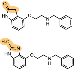
Figure 1: A pair of molecular graphs exhibit the activity cliff phenomena (D van Tilborg, 2022): highly similar structure but dramatic differences in potency.

1 Introduction

Graph Neural Networks (GNNs) (Kipf & Welling, 2017; Veličković et al., 2018), which iteratively propagate learned information in the form of message passing, have recently emerged as powerful approaches on a wide variety of tasks, including drug discovery (Stokes et al., 2020), chip design (Zhang et al., 2019), and catalysts invention (Godwin et al., 2021). Recent studies on GNNs, nevertheless, also reveal a challenge in training GNNs. That is, similar to other successfully deployed deep neural networks, GNNs also require strong model regularization techniques to rectify their over-parameterized learning paradigm.

To this end, various regularization techniques for GNNs have been actively investigated, combating issues such as over-fitting (Zhang et al., 2021), over-smoothing (Li et al., 2018; Wu et al., 2019), and over-squashing (Alon & Yahav, 2021). Despite the complexity of arbitrary structure and topology in graph data, simple edge and node manipulations (e.g., addition and deletion) on graphs (Rong et al., 2020; Zhou et al., 2020; You et al., 2020; Zhao et al., 2021b; Papp et al., 2021) represent a very effective data augmentation strategy, which has been widely used to regularize the learning of GNNs.

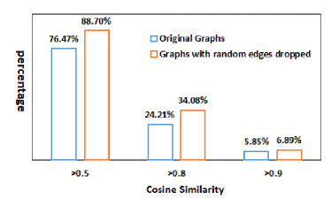
Figure 2: Percentages of graph pairs with certain cosine similarity score but with opposite labels in the NCI1 dataset. This serves as a motivation for careful graph topology modification when conducting graph augmentation for model regularization.

In this paper, we reveal an overlooked issue in the aforementioned graph data augmentation technique for supervised graph classification. That is, simple edge and node manipulations such as addition and deletion can dramatically change the semantics of the original graphs. Consequently, regualarization with such overaggressive graph augmentation methods essentially induces a form of under-fitting, which would inevitably result in the performance degradation of the model. For example, activity cliff phenomena (Maggiora, 2006; D van Tilborg, 2022) has been well observed in molecular graphs. That is, a pair of molecules have highly similar structure but exhibit dramatic differences in potency. Figure 1 visualizes a pair of such molecules (D van Tilborg, 2022). For those molecular pairs, edge or node operation on the graphs risks shifting the functionalities of the molecules, causing overaggressive augmentation.

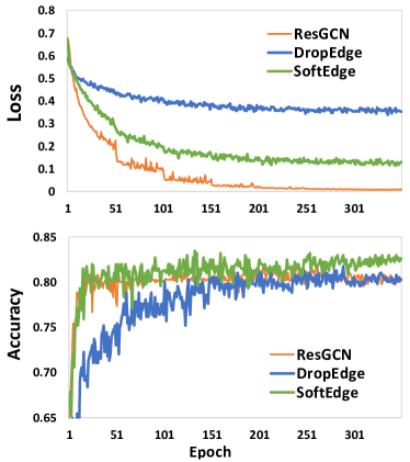
Figure 3: Training loss (top) and validation accuracy (bottom), obtained by ResGCN, DropEdge with 20% edge drop rate, and SoftEdge with 20% soft edges.

Consider, for example, the established benchmark NCI1 dataset (Morris et al., 2020), where each input graph represents a chemical compound with nodes and edges respectively denoting atoms and bonds in a molecule. For such dataset, one can model the Weisfeiler-Lehman graph isomorphism test by comparing the histograms of the node colors of graph pairs in the dataset to demonstrate the activity cliff phenomena. Figure 2 presents the cosine similarity scores of such histograms for all graph pairs with opposite labels both in the original graphs and in the original graphs with randomly dropping 40% of edges. This figure shows that in the original graphs about 5.85% of the graphs with a structure similarity of over 0.9 but with opposite labels, and the percentage increases to 24.21% if we use a cosine similarity threshold of 0.8. Notably, after the random edge dropping, as shown in Figure 2, the percentages of graphs with cosine similarity scores over 0.9 and 0.8 increase to 6.89% and 34.08% respectively. These observations indicate that, in the NCI1 dataset there are many graphs have very similar structures but with different labels, and node and edge modifications may change the semantics of the original graphs and flip the graph labels. We note that in the above motivation analysis, we assume that all edges and nodes are equally important. There also exist scenarios that some graphs are not similar, but changing their key nodes/edges can dramatically change these graphs’ semantic meanings as well, such as removing the hub nodes in social graphs. These observations suggest that graph augmentation should be carefully conducted, and an overaggressive graph augmentation approach can easily result in under-fitting, as will be elaborated next.

In fact, a form of overaggressive regularization has been observed in the popular edge manipulation method DropEdge (Rong et al., 2020), which randomly removes a portion of the edges in a given graph for augmentation. In specific, Figure 3 plots the training loss (top subfigure) and validation accuracy (bottom subfigure) of the ResGCN (Li et al., 2019) and DropEdge (with 20% edge drop rate) methods with 8 layers across the 350 training epochs on the NCI1 dataset. From Figure 3, we can see that ResGCN over-fits the training dataset with close to zero loss, while DropEdge under-fits the training data with a large loss, although their validation accuracy is not too bad. The overaggressive regularization behavior can be further confirmed by the graph embeddings formed. Figure 4 pictures the original training graphs’ embeddings, generated by the trained model of ResGCN as well as DropEdge with 20% and 40% drop rate. We project them to 2D using t-SNE (van der Maaten & Hinton, 2008). From the top, we can see that, the trained model without DropEdge can embed the training graphs into two separable regions for the two classes of the dataset. From the middle subfigures, we can see that, the model trained with DropEdge projects the original training samples to very overlapped embedding regions of the two classes; as the drop rate increases the overlapped regions enlarge. This indeed indicates a form of under-fitting.

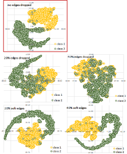
Figure 4: The original training graphs’ 2D embeddings generated by the trained model. Top: ResGCN; Middle: DropEdge with edge drop rate of 20% and 40%. Bottom: SoftEdge with soft edge rate of 20% and 40%.

To address the aforementioned overaggressive augmentation issue caused by dropping/adding graph edges and nodes we propose SoftEdge, which simply assigns random weights in (0, 1) to a portion of the edges of a given graph to generate synthetic graphs. Different to that resulting from DropEdge and DropNode, the synthetic graph generated by SoftEdge has the same nodes and their connectivities as the original graph, thus mitigating the semantic changes during graph augmentation. As shown in Figures 3 (green curve) and  4 (the bottom subfigures), SoftEdge maintains a good trade-off between under-fitting in DropEdge and over-fitting in ResGCN, serving as an effective regularizer for graph classification.

In the experiment section, we further demonstrate, using several benchmark graph classification datasets, that SoftEdge can effectively regularize graph classification learning, resulting in superior accuracy to popular node and edge manipulation approaches and notable resilience to the accuracy degradation in deeper GNNs.

The SoftEdge is easy to be implemented in practice. For example, it can be implemented with the following 6 lines of code in PyTorch Geomertic:

⬇

1. row, _ = data.edge_index #data is the input graphs

2. p = 0.2 # 20% of edges with soft weights

3. softedge = (1- torch.rand((row.size(0),))).to(device)

4. mask = data.edge_index.new_full(

(row.size(0), ), 1 - p, dtype=torch.float)

5. mask = torch.bernoulli(mask)

6. data.edge_weight = softedge*(1-mask)+mask

2 Related Work

Graph data augmentation (Zhao et al., 2021b; Ding et al., 2022b) has been shown to be very effective in regularizing GNNs for generalizing to unseen graphs (Kipf & Welling, 2017; Ying et al., 2018; Veličković et al., 2018; Klicpera et al., 2019b; Xu et al., 2019; Bianchi et al., 2020). Nonetheless, graph data augmentation is rather under-explored due to the arbitrary structure and topology in graphs. Most of such strategies heavily focus on perturbing nodes and edges in graphs (Hamilton et al., 2017; Zhang et al., 2018b; Rong et al., 2020; Chen et al., 2020a; Zhou et al., 2020; Qiu et al., 2020; Wang et al., ; Fu et al., 2020; Wang et al., 2020; Song et al., 2021; Zhao et al., 2021b). For example, DropEdge (Rong et al., 2020) randomly removes a set of edges of a given graph. DropNode, representing node sampling based methods (Hamilton et al., 2017; Chen et al., 2018; Huang et al., 2018), samples a set of nodes from a given graph. DropGNN (Papp et al., 2021) executes multiple GNN runs on the input graph, each with random node dropping. Leveraging sample pairs under the context of Mixup (Zhang et al., 2018a; Guo et al., 2019; Guo, 2020) for graph data augmetation has also been shown to be very promising, including Graph transplant (Park et al., 2022), GraphMixup (Wang et al., 2021) and ifMixup (Guo & Mao, 2021). Compared to the existing works, our study identifies an intrinsic problem in graph data augmentation, namely overaggressive graph augmentation causing under-fitting, which in turn inspires us to devise a novel method, without edge or node deletion/addition, to address this issue in graph augmentation. According to (Ding et al., 2022a; Zhao et al., 2022), the data augmentaiton setting of our method falls in the following category: supervised learning, graph-level classification, edge and node removal and addition.

Graph data augmentation has also been successfully used for contrastive learning  (Chen et al., 2020b; He et al., 2020; You et al., 2020, 2021; Zhu et al., 2020; Suresh et al., 2021; Sun et al., 2021). These methods aim at learning informative graph representations under a self-supervised learning setting. In contrast, we here target a supervised learning setting, aiming to cope with the overaggressive graph augmentation caused by dropping or adding graph edges and nodes.

Our work here is also related to the diffusion processing on the graph adjacency matrix (Klicpera et al., 2019a; Hassani & Khasahmadi, 2020; Zhao et al., 2021a; Chamberlain et al., 2021). Diffusion is a fundamental principle which has been applied to many domains such as image, graph, and physics etc. Compared to the adjacency matrix which focuses on characterizing local information, the diffusion matrix tends to capture global information and needs to be carefully designed. In contrast, instead of capturing the global information as in diffusion models, the equivalent adjacency matrix in SoftEdge tries to retain as much semantics of the original graph as possible by a simple design. Also, leveraging diffusion process to change edge weight would involve careful design of a new learning paradigm, which is in contrast to the simplicity of our proposed method.

3 Augmented Graph with Random Soft Edges

3.1 Graph Classification with Soft Edges

We consider an undirected graph $G=(V,E)$ with the node set $V$ and the edge set $E$. $\mathcal{N}(v)$ represents the neighbours of node $v$, namely the set of nodes in the graph that are directly connected to $v$ in $E$ (i.e., {$u\in V|(u,v)\in E,v\in V\}$). We denote with $N=|V|$ the number of nodes and $A\in\mathbf{R}^{N\times N}$ the adjacency matrix. Each node in $V$ is also associated with a $d$-dimensional feature vector, forming the feature matrix $X\in R^{|V|\times d}$ of the graph. Consider the graph classification task with $C$ categories. Based on a GNN, we aim to learn a mapping function $f:G\rightarrow y$, which assigns a graph $G$ to one of the $C$-class labels $y\in\{1,\dots,C\}$.

Modern GNNs leverage both the graph structure and node features to construct a distributed vector to represent a graph. The forming of such graph representation or embedding follows the “message passing” mechanism for the neighborhood aggregation. In a nutshell, every node starts with the embedding given by its initial features $X(v)$. A GNN then iteratively updates the embedding of a node $h_{v}$ by aggregating representations (i.e., embeddings) of its neighbours layer-by-layer, keep transforming the node embeddings. After the construction of individual node embeddings, the entire graph representation $h_{G}$ can then be obtained through a READOUT function, which aggregates the embeddings of all nodes in the graph.

Formally, the $v$-th node’s representation $h_{v}^{k}$ at the $k$-th layer of a GNN is constructed as follows:

$$h_{v}^{k}=\text{AGGREGATE}(h_{v}^{k-1},{h_{u}^{k-1}|u\in\mathcal{N}(v)},W^{k}),$$ (1)

where $W^{k}$ is the trainable weights at the $k$-th layer; AGGREGATE denotes an aggregation function implemented by the specific GNN model (e.g., the permutation invariant pooling operations Max, Mean, Sum); and $h_{v}^{0}$ is typically initialized as the node input feature $X(v)$.

To provide the graph level representation $h_{G}$, a GNN typically aggregates node representations $h_{v}$ by implementing a READOUT graph pooling function (e.g., Max, Mean, Sum) to summarize information from its individual nodes:

$$h_{G}=\text{READOUT}({h_{v}^{k}|v\in V}).$$ (2)

The final step of the graph classification is to map the graph representation $h_{G}$ to a graph label $y$, through, for example, a softmax layer.

Our proposed SoftEdge leverages graph data with soft edges, which requires the GNN networks be able to take the edge weights into account for message passing when implementing Equation 1 to generate node representations. Fortunately, the two popular GNN networks, namely GCNs (Kipf & Welling, 2017) and GINs (Xu et al., 2019), can naturally take into account the soft edges through weighted summation of neighbor nodes, as follows.

In a GCN, the adjacency matrix can naturally include edge weight values between zero and one (Kipf & Welling, 2017), instead of binary edge weights. Consequently, Equation 1 in a GCN is implemented through a weighted sum operation:

$$\mathbf{h}^{k}_{v}=\sigma\left(W^{k}\cdot\left(\sum_{u\in\mathcal{N}(v)\cup\{v\}}\frac{e_{u,v}}{\sqrt{\hat{d}_{u}\hat{d}_{v}}}\mathbf{h}^{k-1}_{u}\right)\right),$$ (3)

where $\hat{d}_{v}=1+\sum_{u\in\mathcal{N}(v)}e_{u,v}$; $e_{u,v}$ is the edge weight between nodes $u$ and $v$; $W^{k}$ stands for the trainable weights at layer $k$; and $\sigma$ is the non-linearity transformation ReLu.

Similarly, to handle soft edge weights in a GIN, we can simply replace the sum operation of the isomorphism operator with a weighted sum calculation, and get the following implementation of Equation 1 for message passing:

$$\mathbf{h}^{k}_{v}=\text{MLP}^{k}\left((1+\epsilon^{k})\cdot\mathbf{h}_{v}^{k-1}+\sum_{u\in\mathcal{N}(v)}e_{u,v}\cdot\mathbf{h}_{u}^{k-1}\right).$$ (4)

Here, $\epsilon^{k}$ denotes a learnable parameter.

3.2 Graph Learning with Random Soft Edges

Our method SoftEdge takes as input a graph $G=(V,E)$, and a given $\lambda\in(0,1)$ representing the percentage of edges that will be associated with random soft weights. Specifically, at each training epoch, SoftEdge randomly selects $\lambda$ percentage of edges in $E$, and assigns each of the selected edges (denoted as $\widetilde{E}$, $\widetilde{E}\subset E$) with a random weight $w_{\lambda}$ that is uniformly sampled from $(0,1)$.

Assume that all edge weights of the original graph are $1$. With the above operation the newly created synthetic graph will have the same nodes (i.e., $V$) and the edge set (i.e., $E$) as the original graph $G$, except that the edge weights are not all with the value $1$ anymore. In specific, $\lambda$% of edges will be associated with a random weight in $(0,1)$, and the rest will be unchanged. Formally, the edge weights in SoftEdge are as follows:

$$e(u,v)_{w_{\lambda}}=\left\{\begin{array}[]{cl}w_{\lambda},&{\rm if}(u,v)\in\widetilde{E}\\ 1&{\rm otherwise}\end{array}\right.,$$ (5)

where $w_{\lambda}\in(0,1)$, $u,v\in V$, and $\widetilde{E}\subset E$.

This softening edges process is illustrated in Figure 5, where the left subfigure is the original adjacency matrix $A$ for a fully connected graph with self-loop, and the right is the new adjacency matrix $A_{w_{\lambda}}$ generated by SoftEdge, which can be obtained by the dot product between $A$ and the edge weights. The yellow cells are edges with soft weights (belong to edges in $\widetilde{E}$). With such weighted edges, message passing in GNNs as formulated in Equations 3 and  4 can be directly applied for learning.

The pseudo-code of the synthetic graph generation in SoftEdge is described in Algorithm 1.

Algorithm 1 Synthetic graph generation in SoftEdge

Input: a graph $G=(V,E)$ (all edges in $E$ have weight 1); percentage of soft weights $\lambda\in(0,1)$

Output: a synthetic graph $G_{w_{\lambda}}$

Sample $\lambda$ percentage of edges from $E$, forming $\widetilde{E}$

for $(u,v)\in E$ do

    if $(u,v)\in\widetilde{E}$ then

         Sample $w_{\lambda}$ from $(0,1)$ uniformly

         $e(u,v)_{w_{\lambda}}=w_{\lambda}$

    else

         $e(u,v)_{w_{\lambda}}=1$

    end if

end for

Return synthetic graph with new edge weights $e(u,v)_{w_{\lambda}}$

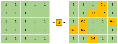
Figure 5: Illustration of SoftEdge: The left is the original adjacency matrix (self-loop; fully connected) with binary weights, and the right is the SoftEdge’s adjacency matrix where $\lambda$% of its elements are in $(0,1)$.

3.3 Discussion

Relation to DropEdge (Rong et al., 2020) The proposed SoftEdge method is inspired by and closely related to DropEdge. Unlike DropEdge, SoftEdge excludes the edge deletion, and instead assigns random weights between $(0,1)$ to a portion of the edges in a graph (SoftEdge would be equivalent to DropEdge if the soft weights were all zero). As a consequence, different from DropEdge, SoftEdge maintains the same nodes and their connectivities as the original graphs in its augmented graphs, thus effectively mitigating the semantic changes during the graph augmentation process.

Why SoftEdge works? Intuitively, GNNs essentially update node embeddings with a weighted sum of the neighborhood information through the graph structure. In SoftEdge, edges of the graph are associated with different weights that are randomly sampled. Consequently, SoftEdge enables a random subset aggregation instead of the fixed neighborhood aggregation during the learning of GNNs, which provides dynamic neighborhood over the graph for message passing. This can be considered as a form of data augmentation or denoising filter, which in turn helps the graph learning because edges in real graphs are often noisy and arbitrarily defined.

More importantly, different from DropEdge, the synthetic graph generated by SoftEdge has the same nodes and their connectivities (i.e., the same $V$ and $E$) as the original graph. The only difference is that the synthetic graph has some soft edges. As such, the synthetic graphs maintain a large similarity to their corresponding original graphs and alleviate the semantic changes during the graph augmentation, which we believe attributes to the superiority of SoftEdge to DropEdge and DropNode.

SoftEdge Improves GNN Expressiveness

Lemma 1

When two different graphs are indistinguishable by the Weisfeiler-Lehman test, assigning random weights to the graphs resolves the ambiguities leading to the failure of the Weisfeiler-Lehman test.

Proof: Due to the random soft edges, each message in the two graphs is transformed differently depending on the weight between the endpoint nodes. As such, the GNN produces the same embedding for the two graphs if we have exactly the same subset of edges with the same random weights, which has the probability zero due to the following fact in SoftEdge: each $w_{\lambda}$ is independently drawn from a continuous distribution over $(0,1)$; hence, the probability of two sets of soft weights $\widetilde{E}_{w_{\lambda}^{i}}$ and $\widetilde{E}_{w_{\lambda}^{j}}$ being identical is zero. Intuitively, the exploiting of graph structure in message passing GNNs can be understood as the breadth first search tree (Xu et al., 2019). Such trees will not be identical when associating some random weights in different tree traversal paths. $\Box$

Sampling in Uniform Distribution It is worth noting that, there is no need to force the soft edge weights to be sampled from a Uniform distribution. For example, one can use a Beta distribution or a Truncated Gaussian.

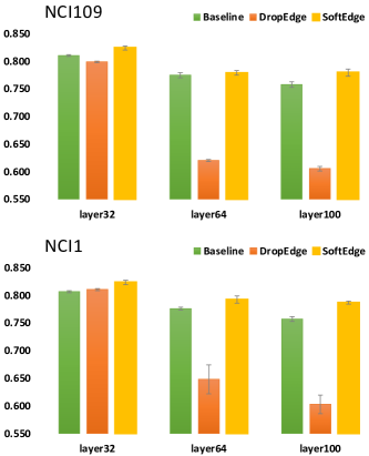
Figure 6: Accuracy obtained by ResGCN, DropEdge, and SoftEdge with 32, 64, and 100 layers on NCI109 and NCI1.

4 Experiments

4.1 Settings

Datasets We conduct experiments using six graph classification tasks from the graph benchmark datasets collection TUDatasets (Morris et al., 2020): PTC_MR, NCI109, NCI1, and MUTAG for small molecule classification, and ENZYMES and PROTEINS for protein categorization. These datasets have been widely used for benchmarking such as in (Xu et al., 2019) and can be downloaded directly using PyTorch Geometric (Fey & Lenssen, 2019)’s built-in function online . Table 1 summarizes the statistics of the datasets, including the number of graphs, the average node number per graph, the average edge number per graph, the number of node features, and the number of classes.

Name	graphs	nodes	edges	features	classes
PTC_MR	334	14.3	29.4	18	2
NCI109	4127	29.7	64.3	38	2
NCI1	4110	29.9	64.6	37	2
MUTAG	188	17.9	39.6	7	2
ENZYMES	600	32.6	124.3	3	6
PROTEINS	1113	39.1	145.6	3	2

Table 1: Statistics of the graph classification benchmark datasets.

Comparison Baselines We compare our method with three baselines: DropEdge (Rong et al., 2020), DropNode (Hamilton et al., 2017; Chen et al., 2018; Huang et al., 2018), and Baseline. For the Baseline model, we use two popular GNN network architectures: GCNs (Kipf & Welling, 2017) and GINs (Xu et al., 2019). GCNs use spectral-based convolutional operation to learn spectral features of graph through message aggregation, leveraging a normalized adjacency matrix. In the experiments, we use the GCN with Skip Connection (He et al., 2016) as that in (Li et al., 2019). Such Skip Connection empowers the GCN to benefit from deeper layers in a GNN. We denote this GCN as ResGCN. The GIN represents the state-of-the-art GNN architecture. It leverages the nodes’ spatial relations to aggregate neighbor features. For both ResGCN and GIN, we use their implementations in the PyTorch Geometric platform .

We note that, in this paper, we aim to study the overaggressive graph augmentation issue in edge and node manipulation. Therefore, we compare our method with commonly used data augmentation baselines DropEdge and DropNode. We believe that, our method is also useful for advanced graph data augmentation strategies, which we will leave for future studies.

Detailed Settings We follow the evaluation protocol and hyperparameters search of GIN (Xu et al., 2019) and DropEdge (Rong et al., 2020). In detail, we evaluate the models using 10-fold cross validation, and compute the mean and standard deviation of three runs. Each fold is trained with 350 epochs with AdamW optimizer (Kingma & Ba, 2015). The initial learning rate is decreased by half every 50 epochs. The hyper-parameters searched for all models on each dataset are as follows: (1) initial learning rate $\in$ {0.01, 0.0005}; (2) hidden unit of size 64; (3) batch size $\in$ {32, 128}; (4) dropout ratio after the dense layer $\in$ {0, 0.5}; (5) drop ratio in DropNode and DropEdge $\in$ {20%, 40%}, (6) number of layers in GNNs $\in$ {3, 5, 8, 16, 32, 64, 100}. For SoftEdge, $\lambda$, the percentage of soft edges, is 20%, and the soft edge weights are uniformly sampled from (0, 1), unless otherwise specified. Following GIN (Xu et al., 2019) and DropEdge (Rong et al., 2020), we report the case giving the best 10-fold average cross-validation accuracy. Our experiments use a NVIDIA V100/32GB GPU.

Dataset	Method	3 layers	5 layers	8 layers	16 layers	max
PTC_MR	ResGCN	0.619$\pm$0.006	0.642$\pm$0.003	0.638$\pm$0.003	0.652$\pm$0.008	0.652
	DropEdge	0.633$\pm$0.006	0.653$\pm$0.007	0.646$\pm$0.002	0.652$\pm$0.005	0.653
	DropNode	0.620$\pm$0.002	0.648$\pm$0.018	0.642$\pm$0.005	0.649$\pm$0.007	0.649
	SoftEdge	0.649$\pm$0.006	0.665$\pm$0.004	0.664$\pm$0.006	0.671$\pm$0.006	0.671
NCI109	ResGCN	0.791$\pm$0.004	0.803$\pm$0.003	0.807$\pm$0.001	0.810$\pm$0.003	0.810
	DropEdge	0.760$\pm$0.000	0.778$\pm$0.008	0.800$\pm$0.002	0.808$\pm$0.003	0.808
	DropNode	0.765$\pm$0.002	0.793$\pm$0.015	0.801$\pm$0.002	0.802$\pm$0.001	0.802
	SoftEdge	0.790$\pm$0.005	0.813$\pm$0.003	0.821$\pm$0.001	0.824$\pm$0.001	0.824
NCI1	ResGCN	0.796$\pm$0.002	0.804$\pm$0.003	0.810$\pm$0.002	0.814$\pm$0.003	0.814
	DropEdge	0.776$\pm$0.001	0.795$\pm$0.010	0.814$\pm$0.001	0.818$\pm$0.001	0.818
	DropNode	0.778$\pm$0.001	0.805$\pm$0.019	0.812$\pm$0.001	0.813$\pm$0.002	0.813
	SoftEdge	0.799$\pm$0.002	0.819$\pm$0.001	0.822$\pm$0.002	0.827$\pm$0.001	0.827
MUTAG	ResGCN	0.827$\pm$0.003	0.841$\pm$0.009	0.846$\pm$0.001	0.846$\pm$0.000	0.846
	DropEdge	0.816$\pm$0.003	0.832$\pm$0.003	0.850$\pm$0.006	0.858$\pm$0.003	0.858
	DropNode	0.823$\pm$0.006	0.829$\pm$0.006	0.839$\pm$0.003	0.858$\pm$0.006	0.858
	SoftEdge	0.859$\pm$0.008	0.841$\pm$0.001	0.846$\pm$0.005	0.874$\pm$0.003	0.874
ENZYMES	ResGCN	0.508$\pm$0.015	0.537$\pm$0.003	0.540$\pm$0.010	0.541$\pm$0.014	0.541
	DropEdge	0.489$\pm$0.003	0.521$\pm$0.003	0.564$\pm$0.011	0.597$\pm$0.002	0.597
	DropNode	0.510$\pm$0.002	0.532$\pm$0.006	0.573$\pm$0.006	0.590$\pm$0.004	0.590
	SoftEdge	0.518$\pm$0.004	0.564$\pm$0.005	0.586$\pm$0.005	0.615$\pm$0.004	0.615
PROTEINS	ResGCN	0.738$\pm$0.005	0.738$\pm$0.002	0.739$\pm$0.003	0.747$\pm$0.005	0.747
	DropEdge	0.747$\pm$0.003	0.750$\pm$0.003	0.749$\pm$0.002	0.755$\pm$0.002	0.755
	DropNode	0.745$\pm$0.004	0.748$\pm$0.001	0.744$\pm$0.002	0.745$\pm$0.005	0.748
	SoftEdge	0.745$\pm$0.002	0.748$\pm$0.000	0.741$\pm$0.000	0.757$\pm$0.003	0.757

Table 2: Accuracy of the testing methods with ResGCN networks as baseline. We report mean accuracy over 3 runs of 10-fold cross validation with standard deviations (denoted $\pm$). Max depicts the max accuracy over different GNN layers. Best results are in Bold.

4.2 Results with ResGCN

4.2.1 Main Results

Table 2 presents the accuracy obtained by the ResGCN (Kipf & Welling, 2017; Li et al., 2019) baseline, DropEdge, DropNode, and SoftEdge on the six datasets, where we evaluate GNNs with 3, 5, 8, and 16 layers. In the table, the best results are in Bold.

Results in the last column of Table 2 show that SoftEdge outperformed all the three comparison models on all the six datasets when considering the max accuracy obtained with layers 3, 5, 8, and 16. For example, when compared with ResGCN, SoftEdge increased the accuracy from 65.2%, 84.6%, and 54.1% to 67.1%, 87.4%, and 61.5%, respectively, on the PTC_MR, MUTAG, and ENZYMES datasets. Similarly, when compared with DropEdge, SoftEdge improved the accuracy from 65.3%, 80.8%, and 84.6% to 67.1%, 82.4%, and 87.4%, respectively, on the PTC_MR, NCI109, and MUTAG datasets.

Promisingly, as highlighted in bold in the table, SoftEdge obtained superior accuracy to the other comparison models in most settings regardless of the network layers used. For example, on the PTC_MR, NCI1, and ENZYMES datasets, SoftEdge outperformed all the three baselines with all the network depths tested (i.e., 3, 5, 8, and 16 layers).

Another observation here is that SoftEdge improved or maintained the predictive accuracy in most of the cases as the networks increased their depth from 3, 5, 8, to 16. As can be seen in Table 2, the best accuracy of SoftEdge on all the six datasets were obtained by SoftEdge with 16 layers.

4.2.2 Ablation Studies

We conduct ablation studies to evaluate SoftEdge. We particularly compare our strategy with DropEdge, since it is the most related algorithm to our approach.

Effect on GNN Depth We conduct experiments on further increasing the networks’ depth by adding more layers, including ResGCN with 32, 64, and 100 layers. Results on the NCI109 and NCI1 datasets are presented in Figure 6.

Results in Figure 6 show that DropEdge significantly degraded the predictive accuracy when ResGCN has 64 and 100 layers; and surprisingly, the baseline model ResGCN performed better than DropEdge as the networks went deeper. Notably, the SoftEdge method was able to slow down the degradation in terms of the accuracy obtained with deeper networks, outperforming both baselines ResGCN and DropEdge with layers 32, 64, and 100.

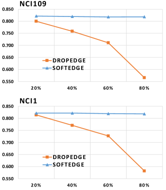
Figure 7: Accuracy obtained by DropEdge and SoftEdge as ratio of modified edges (x-axis) increasing on NCI109 and NCI1.

Ratio of Modified Edges In Figure 7, we present the results when varying the percentage of modified edges (i.e., $\lambda$) in both DropEdge and SoftEdge with 8 layers. We evaluate the percentage of 20%, 40%, 60%, and 80%, respectively, on NCI109 and NCI1. We chose these two datasets since they have the largest number of node features amongst the six tested datasets, which are more challenging. This is because, intuitively with a large number of node features the overaggressive augmentation issue could be mitigated.

Results in Figure 7 show that, DropEdge was very sensitive to the percentage of modified edges as the model’s predictive accuracy decreases significantly with the drop rate. This is expected, as DropEdge completely dropped selected edges the graph structure would be largely changed especially when the drop rate is high. On the other hand, SoftEdge seemed to be robust to the percentage of edges being modified as the accuracy obtained for the candidate ratios was quite similar. This is mainly because, unlike DropEdge, the synthetic graphs generated by SoftEdge remain a large similarity to the original graphs as the node structures are kept the same.

Dataset	Method	5 layers	8 layers	16 layers	max
PTC_MR	GIN	0.647$\pm$0.005	0.659$\pm$0.003	0.673$\pm$0.022	0.673
	DropEdge	0.680$\pm$0.003	0.681$\pm$0.009	0.679$\pm$0.007	0.681
	DropNode	0.688$\pm$0.006	0.689$\pm$0.003	0.680$\pm$0.006	0.689
	SoftEdge	0.687$\pm$0.011	0.691$\pm$0.009	0.696$\pm$0.007	0.696
NCI109	GIN	0.818$\pm$0.002	0.823$\pm$0.002	0.820$\pm$0.001	0.823
	DropEdge	0.813$\pm$0.005	0.814$\pm$0.003	0.805$\pm$0.003	0.814
	DropNode	0.819$\pm$0.002	0.821$\pm$0.002	0.816$\pm$0.004	0.821
	SoftEdge	0.835$\pm$0.002	0.836$\pm$0.001	0.838$\pm$0.003	0.838
NCI1	GIN	0.820$\pm$0.002	0.821$\pm$0.001	0.821$\pm$0.002	0.821
	DropEdge	0.819$\pm$0.004	0.823$\pm$0.001	0.818$\pm$0.003	0.823
	DropNode	0.821$\pm$0.003	0.821$\pm$0.003	0.824$\pm$0.000	0.824
	SoftEdge	0.839$\pm$0.001	0.839$\pm$0.002	0.837$\pm$0.005	0.839
MUTAG	GIN	0.876$\pm$0.003	0.871$\pm$0.003	0.874$\pm$0.000	0.876
	DropEdge	0.857$\pm$0.005	0.878$\pm$0.009	0.871$\pm$0.003	0.878
	DropNode	0.864$\pm$0.006	0.875$\pm$0.003	0.869$\pm$0.009	0.875
	SoftEdge	0.876$\pm$0.006	0.878$\pm$0.005	0.889$\pm$0.005	0.889
ENZYMES	GIN	0.531$\pm$0.004	0.533$\pm$0.006	0.532$\pm$0.001	0.533
	DropEdge	0.480$\pm$0.003	0.497$\pm$0.013	0.487$\pm$0.004	0.497
	DropNode	0.521$\pm$0.004	0.563$\pm$0.005	0.552$\pm$0.004	0.563
	SoftEdge	0.571$\pm$0.002	0.590$\pm$0.003	0.588$\pm$0.009	0.590
PROTEINS	GIN	0.741$\pm$0.006	0.744$\pm$0.005	0.743$\pm$0.001	0.744
	DropEdge	0.742$\pm$0.002	0.738$\pm$0.004	0.736$\pm$0.003	0.742
	DropNode	0.736$\pm$0.002	0.745$\pm$0.002	0.747$\pm$0.002	0.747
	SoftEdge	0.740$\pm$0.002	0.742$\pm$0.004	0.747$\pm$0.002	0.747

Table 3: Accuracy of the testing methods with GIN networks as baseline. We report mean accuracy over 3 runs of 10-fold cross validation with standard deviations (denoted $\pm$). Max depicts the max accuracy over different GNN layers. Best results are in Bold.

4.3 Results with GIN

In this section, we also evaluate our method using the GIN (Xu et al., 2019) network architecture. Table 3 presents the accuracy obtained by the GIN, DropEdge, DropNode, and SoftEdge on the six datasets, where we examine GNNs with 5, 8, and 16 layers and the best results are in Bold.

Results in Table 3 show that, similar to the ResGCN case, SoftEdge with GIN as the baseline outperformed all the other comparison models on all the six datasets, as highlighted by the last column of the table. For example, when compared with the GIN baseline, SoftEdge increased the accuracy from 67.3%, 82.1%, and 53.3% to 69.6%, 83.9%, and 59.0%, respectively, on the PTC_MR, NCI1, and ENZYMES datasets. Similarly, when compared with DropEdge, SoftEdge improved the accuracy from 81.4%, 82.3%, and 49.7% to 83.8%, 83.9%, and 59.0%, respectively, on the NCI109, NCI1, and ENZYMES datasets.

We note that our work here aims at studying and addressing the overaggressive graph augmentation issues caused by the widely used edge and node dropping on supervised graph classification. We conjecture that on the node level classification, we may also have graph nodes with very similar neighbourhoods but of different node labels, owing to the node and edge operation in the augmentation processes. Nevertheless, the aggressive augmentation issue is more complex on node level due to the over-smoothing phenomena (Li et al., 2018; Wu et al., 2019), where the representations of all nodes in a graph may converge to a subspace that makes their representations unrelated to the graph input (Li et al., 2018; Wu et al., 2019). We intend to study such node classification in the future.

5 Conclusions and Future Work

We discussed the overaggressive graph augmentation issue in simple edge and node manipulations for graph regularization, where the semantics of augmented graphs may differ from their original graphs, which will induce a form of under-fitting for model regularization. We proposed SoftEdge, which assigns random weights to a portion of the edges of a given graph, enabling training GNNs with dynamic neighborhoods. The synthetic graph generated by SoftEdge maintains the same nodes and their connectivities as the original graph, thus mitigating the semantics changes of the original graph. We also showed that this simple approach resulted in superior accuracy to popular node and edge manipulation methods and notable resilience to the accuracy degradation with the GNN depth.

We note that SoftEdge assumes that the given graphs for training have binary edges, which is a commonly adopted setting in the graph learning field. When using graphs with real-valued edge weights, there are two main strategies to handle such situation in the literature, which can be adopted by our SoftEdge algorithm. In the first method, edge weights are added to the features of the nodes (Hu et al., 2020a; Li et al., 2020). In the second approach, edge weights are treated the same way as node features in the Aggregation function of the GNNs (Gilmer et al., 2017; Xu et al., 2019; Kipf & Welling, 2017; Hu et al., 2020b). It is also worth noting that these two approaches can also be used by SoftEdge for graphs that are associated with edge attributes.

References

- Alon & Yahav (2021) Alon, U. and Yahav, E. On the bottleneck of graph neural networks and its practical implications. In International Conference on Learning Representations, 2021.
- Bianchi et al. (2020) Bianchi, F. M., Grattarola, D., and Alippi, C. Spectral clustering with graph neural networks for graph pooling. In Proceedings of the 37th international conference on Machine learning, pp. 2729–2738. ACM, 2020.
- Chamberlain et al. (2021) Chamberlain, B. P., Rowbottom, J., Gorinova, M. I., Webb, S. D., Rossi, E., and Bronstein, M. M. GRAND: Graph neural diffusion. In The Symbiosis of Deep Learning and Differential Equations, 2021. URL https://openreview.net/forum?id=_1fu_cjsaRE.
- Chen et al. (2020a) Chen, D., Lin, Y., Li, W., Li, P., Zhou, J., and Sun, X. Measuring and relieving the over-smoothing problem for graph neural networks from the topological view. In The Thirty-Fourth AAAI Conference on Artificial Intelligence, pp. 3438–3445. AAAI Press, 2020a.
- Chen et al. (2018) Chen, J., Ma, T., and Xiao, C. Fastgcn: Fast learning with graph convolutional networks via importance sampling. CoRR, 2018.
- Chen et al. (2020b) Chen, T., Kornblith, S., Norouzi, M., and Hinton, G. A simple framework for contrastive learning of visual representations, 2020b.
- D van Tilborg (2022) D van Tilborg, A Alenicheva, G. G. Exposing the limitations of molecular machine learning with activity cliffs. 2022.
- Ding et al. (2022a) Ding, K., Xu, Z., Tong, H., and Liu, H. Data augmentation for deep graph learning: A survey. 2022a.
- Ding et al. (2022b) Ding, K., Xu, Z., Tong, H., and Liu, H. Data augmentation for deep graph learning: A survey. arXiv, 2022b.
- Fey & Lenssen (2019) Fey, M. and Lenssen, J. E. Fast graph representation learning with PyTorch Geometric. In ICLR Workshop on Representation Learning on Graphs and Manifolds, 2019.
- Fu et al. (2020) Fu, K., Mao, T., Wang, Y., Lin, D., Zhang, Y., Zhan, J., an Sun, X., and Li, F. Ts-extractor: large graph exploration via subgraph extraction based on topological and semantic information. Journal of Visualization, pp. 1 – 18, 2020.
- Gilmer et al. (2017) Gilmer, J., Schoenholz, S. S., Riley, P. F., Vinyals, O., and Dahl, G. E. Neural message passing for quantum chemistry. CoRR, abs/1704.01212, 2017.
- Godwin et al. (2021) Godwin, J., Schaarschmidt, M., Gaunt, A., Sanchez-Gonzalez, A., Rubanova, Y., Veličković, P., Kirkpatrick, J., and Battaglia, P. Very deep graph neural networks via noise regularisation, 2021.
- Guo (2020) Guo, H. Nonlinear mixup: Out-of-manifold data augmentation for text classification. Proceedings of the AAAI Conference on Artificial Intelligence, pp. 4044–4051, Apr. 2020.
- Guo & Mao (2021) Guo, H. and Mao, Y. Intrusion-free graph mixup. arXiv, 2021.
- Guo et al. (2019) Guo, H., Mao, Y., and Zhang, R. Mixup as locally linear out-of-manifold regularization. In AAAI, 2019.
- Hamilton et al. (2017) Hamilton, W. L., Ying, R., and Leskovec, J. Inductive representation learning on large graphs. NIPS’17, 2017.
- Hassani & Khasahmadi (2020) Hassani, K. and Khasahmadi, A. H. Contrastive multi-view representation learning on graphs. In Advances in International Conference on Machine Learning, 2020. URL https://proceedings.mlr.press/v119/hassani20a/hassani20a.pdf.
- He et al. (2016) He, K., Zhang, X., Ren, S., and Sun, J. Deep residual learning for image recognition. In 2016 IEEE Conference on Computer Vision and Pattern Recognition (CVPR), 2016.
- He et al. (2020) He, K., Fan, H., Wu, Y., Xie, S., and Girshick, R. Momentum contrast for unsupervised visual representation learning, 2020.
- Hu et al. (2020a) Hu, W., Fey, M., Zitnik, M., Dong, Y., Ren, H., Liu, B., Catasta, M., and Leskovec, J. Open graph benchmark: Datasets for machine learning on graphs. CoRR, 2020a.
- Hu et al. (2020b) Hu, W., Liu, B., Gomes, J., Zitnik, M., Liang, P., Pande, V., and Leskovec, J. Strategies for pre-training graph neural networks, 2020b.
- Huang et al. (2018) Huang, W., Zhang, T., Rong, Y., and Huang, J. Adaptive sampling towards fast graph representation learning. 2018.
- Kingma & Ba (2015) Kingma, D. P. and Ba, J. Adam: A method for stochastic optimization. In Bengio, Y. and LeCun, Y. (eds.), 3rd International Conference on Learning Representations, ICLR 2015, San Diego, CA, USA, May 7-9, 2015, Conference Track Proceedings, 2015.
- Kipf & Welling (2017) Kipf, T. N. and Welling, M. Semi-supervised classification with graph convolutional networks. In International Conference on Learning Representations (ICLR), 2017.
- Klicpera et al. (2019a) Klicpera, J., Weißenberger, S., and Günnemann, S. Diffusion improves graph learning. CoRR, abs/1911.05485, 2019a.
- Klicpera et al. (2019b) Klicpera, J., Weißenberger, S., and Günnemann, S. Diffusion improves graph learning. In Conference on Neural Information Processing Systems (NeurIPS), 2019b.
- Li et al. (2019) Li, G., Müller, M., Thabet, A., and Ghanem, B. Deepgcns: Can gcns go as deep as cnns? In The IEEE International Conference on Computer Vision (ICCV), 2019.
- Li et al. (2020) Li, G., Xiong, C., Thabet, A. K., and Ghanem, B. Deepergcn: All you need to train deeper gcns. CoRR, abs/2006.07739, 2020.
- Li et al. (2018) Li, Q., Han, Z., and Wu, X. Deeper insights into graph convolutional networks for semi-supervised learning. In McIlraith, S. A. and Weinberger, K. Q. (eds.), AAAI, 2018.
- Maggiora (2006) Maggiora, G. On outliers and activity cliffs - why qsar often dissapoints. Journal of chemical information and modeling, 46:1535, 07 2006. doi: 10.1021/ci060117s.
- Morris et al. (2020) Morris, C., Kriege, N. M., Bause, F., Kersting, K., Mutzel, P., and Neumann, M. Tudataset: A collection of benchmark datasets for learning with graphs. In ICML 2020 Workshop on Graph Representation Learning and Beyond (GRL+ 2020), 2020.
- Papp et al. (2021) Papp, P. A., Martinkus, K., Faber, L., and Wattenhofer, R. DropGNN: Random dropouts increase the expressiveness of graph neural networks. In Beygelzimer, A., Dauphin, Y., Liang, P., and Vaughan, J. W. (eds.), Advances in Neural Information Processing Systems, 2021.
- Park et al. (2022) Park, J., Shim, H., and Yang, E. Graph transplant: Node saliency-guided graph mixup with local structure preservation. In AAAI, 2022.
- Qiu et al. (2020) Qiu, J., Chen, Q., Dong, Y., Zhang, J., Yang, H., Ding, M., Wang, K., and Tang, J. GCC: Graph Contrastive Coding for Graph Neural Network Pre-Training, pp. 1150–1160. 2020.
- Rong et al. (2020) Rong, Y., Huang, W., Xu, T., and Huang, J. Dropedge: Towards deep graph convolutional networks on node classification. In International Conference on Learning Representations, 2020.
- Song et al. (2021) Song, R., Giunchiglia, F., Zhao, K., and Xu, H. Topological regularization for graph neural networks augmentation. CoRR, abs/2104.02478, 2021.
- Stokes et al. (2020) Stokes, J. M., Yang, K., Swanson, K., Jin, W., Cubillos-Ruiz, A., Donghia, N. M., MacNair, C. R., French, S., Carfrae, L. A., Bloom-Ackermann, Z., et al. A deep learning approach to antibiotic discovery. Cell, 180(4):688–702, 2020.
- Sun et al. (2021) Sun, M., Xing, J., Wang, H., Chen, B., and Zhou, J. Mocl: Data-driven molecular fingerprint via knowledge-aware contrastive learning from molecular graph. In Zhu, F., Ooi, B. C., and Miao, C. (eds.), KDD ’21: The 27th ACM SIGKDD Conference on Knowledge Discovery and Data Mining, Virtual Event, Singapore, August 14-18, 2021, 2021.
- Suresh et al. (2021) Suresh, S., Li, P., Hao, C., and Neville, J. Adversarial graph augmentation to improve graph contrastive learning. In Beygelzimer, A., Dauphin, Y., Liang, P., and Vaughan, J. W. (eds.), Advances in Neural Information Processing Systems, 2021.
- van der Maaten & Hinton (2008) van der Maaten, L. and Hinton, G. Visualizing data using t-sne. Journal of Machine Learning Research, 9(86):2579–2605, 2008.
- Veličković et al. (2018) Veličković, P., Cucurull, G., Casanova, A., Romero, A., Liò, P., and Bengio, Y. Graph Attention Networks. International Conference on Learning Representations, 2018.
- (43) Wang, Y., Wang, W., Liang, Y., Cai, Y., Liu, J., and Hooi, B. Nodeaug: Semi-supervised node classification with data augmentation. In Gupta, R., Liu, Y., Tang, J., and Prakash, B. A. (eds.), KDD ’20, pp. 207–217.
- Wang et al. (2020) Wang, Y., Wang, W., Liang, Y., Cai, Y., and Hooi, B. Graphcrop: Subgraph cropping for graph classification. CoRR, abs/2009.10564, 2020.
- Wang et al. (2021) Wang, Y., Wang, W., Liang, Y., Cai, Y., and Hooi, B. Mixup for node and graph classification. In Proceedings of the Web Conference 2021, pp. 3663–3674, 2021.
- Wu et al. (2019) Wu, Z., Pan, S., Chen, F., Long, G., Zhang, C., and Yu, P. S. A comprehensive survey on graph neural networks. CoRR, 2019.
- Xu et al. (2019) Xu, K., Hu, W., Leskovec, J., and Jegelka, S. How powerful are graph neural networks? In International Conference on Learning Representations, 2019.
- Ying et al. (2018) Ying, Z., You, J., Morris, C., Ren, X., Hamilton, W. L., and Leskovec, J. Hierarchical graph representation learning with differentiable pooling. In NeurIPS 2018, pp. 4805–4815, 2018.
- You et al. (2020) You, Y., Chen, T., Sui, Y., Chen, T., Wang, Z., and Shen, Y. Graph contrastive learning with augmentations. In Larochelle, H., Ranzato, M., Hadsell, R., Balcan, M. F., and Lin, H. (eds.), NeurIPs, volume 33, pp. 5812–5823. Curran Associates, Inc., 2020.
- You et al. (2021) You, Y., Chen, T., Shen, Y., and Wang, Z. Graph contrastive learning automated. ICML21, 2021.
- Zhang et al. (2021) Zhang, C., Bengio, S., Hardt, M., Recht, B., and Vinyals, O. Understanding deep learning (still) requires rethinking generalization. 2021.
- Zhang et al. (2019) Zhang, G., He, H., and Katabi, D. Circuit-gnn: Graph neural networks for distributed circuit design. In International Conference on Machine Learning, 2019.
- Zhang et al. (2018a) Zhang, H., Cissé, M., Dauphin, Y. N., and Lopez-Paz, D. mixup: Beyond empirical risk minimization. In ICLR2018, 2018a.
- Zhang et al. (2018b) Zhang, Y., Pal, S., Coates, M., and Üstebay, D. Bayesian graph convolutional neural networks for semi-supervised classification. 2018b.
- Zhao et al. (2021a) Zhao, J., Dong, Y., Ding, M., Kharlamov, E., and Tang, J. Adaptive diffusion in graph neural networks. In Beygelzimer, A., Dauphin, Y., Liang, P., and Vaughan, J. W. (eds.), Advances in Neural Information Processing Systems, 2021a.
- Zhao et al. (2021b) Zhao, T., Liu, Y., Neves, L., Woodford, O., Jiang, M., and Shah, N. Data augmentation for graph neural networks. In Proceedings of the AAAI Conference on Artificial Intelligence, volume 35, pp. 11015–11023, 2021b.
- Zhao et al. (2022) Zhao, T., Liu, G., Günneman, S., and Jiang, M. Graph data augmentation for graph machine learning: A survey. arXiv preprint arXiv:2202.08871, 2022.
- Zhou et al. (2020) Zhou, J., Shen, J., and Xuan, Q. Data augmentation for graph classification. In Proceedings of the 29th ACM International Conference on Information and Knowledge Management, pp. 2341–2344, 2020.
- Zhu et al. (2020) Zhu, Y., Xu, Y., Yu, F., Liu, Q., Wu, S., and Wang, L. Graph Contrastive Learning with Adaptive Augmentation. arXiv e-prints, 2020.