Lattice and Non-lattice Piercing of Axis-Parallel Rectangles:
Exact Algorithms and a Separation Result

Abstract

For a given family of shapes $\mathcal{F}$ in the plane, we study what is the lowest possible density of a point set $P$ that pierces (“intersects”, “hits”) all translates of each shape in $\mathcal{F}$. For instance, if $\mathcal{F}$ consists of two axis-parallel rectangles the best known piercing set, i.e., one with the lowest density, is a lattice: for certain families the known lattices are provably optimal whereas for other, those lattices are just the best piercing sets currently known.

Given a finite family $\mathcal{F}$ of axis-parallel rectangles, we present two algorithms for finding an optimal $\mathcal{F}$-piercing lattice. Both algorithms run in time polynomial in the number of rectangles and the maximum aspect ratio of the rectangles in the family. No prior algorithms were known for this problem.

Then we prove that for every $n\geq 3$, there exist a family of $n$ axis-parallel rectangles for which the best piercing density achieved by a lattice is separated by a positive (constant) gap from the optimal piercing density for the respective family. Finally, we sharpen our separation result by running the first algorithm on a suitable instance, and show that the best lattice can be sometimes worse by $20\%$ than the optimal piercing set.

Keywords: axis-parallel rectangle, piercing set, piercing lattice, canonical vector basis, periodic tiling, exact algorithm, approximation algorithm.

1 Introduction

Piercing and covering are interrelated ubiquitous topics in geometry. Given a family of sets $\mathbb{E}$ in the Euclidean space, a piercing set is a set of points in $\mathbb{R}^{d}$ collectively intersecting every set in $\mathbb{E}$. If $\mathbb{E}$ contains an infinite subfamily consisting of pairwise disjoint members then clearly every piercing set for $\mathbb{E}$ must be infinite as well. Given a finite family of shapes $\mathcal{F}$ in the plane, what is the lowest possible density of a point set $P$ that pierces (“intersects”, “hits”) all translates of each shape in $\mathcal{F}$? Regardless of what $\mathcal{F}$ is, such a set must be infinite. In this paper we consider this problem for families $\mathcal{F}$ of axis-parallel rectangles where the goal is finding a point set of minimum density $\pi_{T}(\mathcal{F})$ that collectively pierces each translate of a rectangle in $\mathcal{F}$. The problem was introduced in [4], where an approximation algorithm and several other results have been obtained for such families.

If $\mathcal{F}$ consists of a single axis-parallel rectangle $R$, an optimal piercing set is a rectangular lattice given by a tiling of the plane with copies of $R$ (i.e., a covering of the plane by interior-disjoint translates of $R$). If $\mathcal{F}$ consists of two axis-parallel rectangles, the answer is unknown! The best piercing set currently known in this setting, i.e., one with the lowest density, is a lattice: for certain families of two rectangles, the known lattices are provably optimal whereas for others, the answer remains elusive [4]. As such, the question posed above appears as a basic open problem.

The starting point of this paper is the observation that for certain families $\mathcal{F}$ of axis-parallel rectangles, there exist surprisingly sparse $\mathcal{F}$-piercing point sets that are not lattices. For instance, for the family $\mathcal{F}=\{6\times 1,1\times 6,3\times 3\}$ there exists a periodic $\mathcal{F}$-piercing non-lattice set with the (optimal) density $1/6$; see Fig. 1. The indicated piercing set is a subset of the integer lattice $\mathbb{Z}^{2}$ and so the verification of the piercing property can be done visually and is left to the reader. Building up on the above observation we prove that no lattice with density $1/6$ is $\mathcal{F}$-piercing, i.e., the sparsest lattice is sometimes strictly worse than the sparsest point set, i.e., $\pi_{L}(\mathcal{F})>\pi(F)$. Moreover, we prove a separation result showing that the sparsest lattice is sometimes significantly worse than the sparsest point set. This last step requires a careful setup (see properties P1–P3 below).

Setup.

Let $\mathcal{F}=\{R_{1},\dots,R_{n}\}$ be a family of axis-parallel rectangles $R_{i}=w_{i}\times h_{i}$. Without loss of generality (after suitable scaling) we may assume that (i) the minimum rectangle width and height are both $1$; i.e., $\min w_{i}=1$, and $\min h_{i}=1$; and (ii) no input rectangle is contained in another. We further set $k=\max\{w,h\}$, where $w=\max\{w_{i}\}$ and $h=\max\{h_{i}\}$, i.e., $k$ is the maximum dimension (extent) of a rectangle in $\mathcal{F}$.

As a first step, we will show how to find a canonical vector basis $[u,v]$ for any lattice $\Lambda$; this may require a reflection of the $x$-axis and a $90^{\circ}$ rotation of the lattice and the rectangles. Such a basis satisfies the following three properties (we have opted for $b>0$ since this would be the case for the integer lattice with $a,b,c,d=0,1,1,0$). Consequently, all our algorithms work with or rely on the existence of such a basis.

1. if $u$ is a shortest vector in $\Lambda$, then $u$ has positive (or $\infty$) slope and $v$ has negative (or $0$) slope, i.e., $u=[a,b]$, $v=[c,-d]$ with $a,b,c,d\geq 0$, and $b>0$.

2. $1/2\leq|u|\leq|v|\leq\sqrt{\frac{7}{3}}\,\frac{A}{\lambda}$, where $\lambda=|u|$ and $A=ad+bc$ is the area of a fundamental parallelogram of $\Lambda$.

3. the angle $\alpha$ between $u$ and $v$ is between $45^{\circ}$ and $135^{\circ}$.

Definitions and notations.

Given a point set $P$ and a bounded domain $D$ with area $\text{Area}(D)$, we define the density of $P$ over $D$ by $\delta(P,D)=\frac{|P\cap D|}{\text{Area}(D)}$. In particular, the density of a point lattice is the reciprocal of the determinant $\det[u,v]$, where $[u,v]$ is a vector basis of the lattice [1, p. 2].

Outline.

In Section 3 we show the existence of a canonical vector basis (satisfying properties P1–P3). For lattices satisfying P1–P3, in Section 4 we present a decision algorithm: given a family $\mathcal{F}$ and a canonical vector basis the decision algorithm determines if the corresponding lattice is $\mathcal{F}$-piercing. In Section 5 we present two algorithms for computing an optimal $\mathcal{F}$-piercing lattice: given a family $\mathcal{F}$, each of the two algorithms finds an optimal $\mathcal{F}$-piercing lattice. The key for these algorithms is the fact that candidate lattices must be tight (in a sense that will be made precise). Each of the two algorithms uses the decision algorithm as a subroutine. In the second part of the paper we analyze lattice piercing versus non-lattice piercing and demonstrate explicit instances for which an optimal piercing lattice is non-optimal over all piercing sets.

Our results.

The first result is a decision algorithm. Recall that $k$ is the maximum width or height of a rectangle in $\mathcal{F}$.

Theorem 1.

Given a family $\mathcal{F}=\{R_{1},\dots,R_{n}\}$ consisting of $n$ axis-parallel rectangles, and a canonical vector basis $[u,v]$ of a lattice $\Lambda$, there is an algorithm that determines whether $\Lambda$ is an $\mathcal{F}$-piercing lattice in $\mathcal{O}((k+n)\log{k})$ time.

The existence of a decision algorithm allows us to obtain two algorithms for computing an optimal piercing lattice. Both algorithms employ the decision algorithm in Theorem 1 as a subroutine. Our first algorithm computes an optimal piercing lattice by generating and solving linear systems with two variables.

Theorem 2.

Given a family $\mathcal{F}=\{R_{1},\dots,R_{n}\}$ consisting of $n$ axis-parallel rectangles, an optimal $\mathcal{F}$-piercing lattice can be found in $\mathcal{O}\left(k^{8}n^{4}(n+k)\log{k}\right)$ time.

For rectangles with integer side-lengths we give a simpler algorithm that does not solve any linear systems but uses structural properties of the underlying systems.

Theorem 3.

Given a family $\mathcal{F}=\{R_{1},\dots,R_{n}\}$ consisting of $n$ axis-parallel rectangles with integer dimensions, an optimal $\mathcal{F}$-piercing lattice can be found in $\mathcal{O}\left(k^{18}(k+n)\log{k}\right)$ time.

Note that for rectangles with integer side-lengths we have $n\leq k^{2}$. So when $k=\mathcal{O}(1)$, both algorithms run in $\mathcal{O}(1)$ time on rectangles with integer side-lengths.

In the second part of the paper we analyze lattice piercing versus non-lattice piercing and demonstrate explicit instances for which an optimal piercing lattice is non-optimal over all piercing sets. While the resulting separation is small, its proof is nontrivial.

Theorem 4.

There exists a family $\mathcal{F}_{0}$ of $3$ axis-parallel rectangles and a positive constant $\varepsilon>0$ where the best piercing density achieved by a lattice is at least $\pi(F_{0})+\varepsilon$.

The proof of Theorem 4 yields a value $\varepsilon=3\cdot 10^{-7}$. In the final part of the paper (Sections 8 and 9) we manage to amplify the separation result by roughly six orders of magnitude via computer-assisted proofs.

Theorem 5.

There exists a family $\mathcal{F}_{0}$ of $3$ axis-parallel rectangles for which the best piercing density achieved by a lattice is at least $\frac{36}{31}\pi(F_{0})=(1.161\ldots)\,\pi(F_{0})$.

Theorem 6.

There exists a family $\mathcal{F}_{1}$ of $5$ axis-parallel rectangles for which the best piercing density achieved by a lattice is at least $\frac{6}{5}\,\pi(F_{1})$.

Theorems 4, 5 and 6 can be extended to any larger number of rectangles. Consequently, we obtain the following general separation result.

Theorem 7.

For every $n\geq 5$, there exists a family $\mathcal{F}$ of $n$ axis-parallel rectangles for which the best piercing density achieved by a lattice is at least $\frac{6}{5}\,\pi(F)$.

Related result.

To put Theorem 7 in perspective we point out that from the other direction the following approximation result has been recently obtained. We in fact use this approximation algorithm as a subroutine in our exact algorithm for finding an optimal piercing lattice.

Theorem 8.

[4] Given a family $\mathcal{F}=\{R_{1},\dots,R_{n}\}$ consisting of $n$ axis-parallel rectangles, a $1.895$-approximation of $\pi_{T}(\mathcal{F})$ can be computed in $\mathcal{O}(n)$ time. The output piercing set is a lattice with density at most $(1+\frac{2}{5}\sqrt{5})\cdot\pi_{T}(\mathcal{F})=(1.895\ldots)\cdot\pi_{T}(\mathcal{F})$.

Other related work.

Let $\mathcal{F}$ be a finite family of axis-parallel rectangles. The problem of determining whether a given (infinite) point set $P$ is $\mathcal{F}$-piercing, which is one of the problems we consider here, is closely related to that of determining all maximal empty rectangles amidst the points in $P$. Indeed, a point set $P$ is $\mathcal{F}$-piercing if and only if there is no maximal empty rectangle amidst the points in $P$ strictly containing one of the rectangles from $\mathcal{F}$ in its interior. Note that infinite point sets may allow short descriptions, for instance periodic sets and lattice sets in particular. See for instance the monograph by Grünbaum and Shephard [6] for a discussion of periodic tilings.

It is known that the number of maximal empty rectangles amidst $n$ points is $O(n^{2})$, and this bound is tight [7]. Given an axis-parallel rectangle $R$ in the plane containing $n$ points, the problem of computing a maximum-area empty axis-parallel sub-rectangle contained in $R$ has been studied extensively. Recently, an essentially asymptotically optimal algorithm running in nearly $\mathcal{O}(n\log{n})$ time has been designed by Chan [2].

Let $\mathcal{F}$ be a finite family of axis-parallel rectangles. The piercing number of $\mathcal{F}$, denoted $\tau(\mathcal{F})$, is the minimum cardinality of an $\mathcal{F}$-piercing set. The independence number or matching number of $\mathcal{F}$, namely the maximum number of pairwise disjoint sets in $\mathcal{F}$, is denoted by $\alpha(\mathcal{F})$ or $\nu(\mathcal{F})$. Clearly, $\nu(\mathcal{F})\leq\tau(\mathcal{F})$. The main unsettled question here is whether $\tau(\mathcal{F})=\mathcal{O}(\nu(\mathcal{F}))$. The best known upper bound is due to Correa et al. [3].

2 Non-lattice periodic piercing

Figure 1 below shows a non-lattice periodic grid point-set that pierces all translates of rectangles in $\mathcal{F}_{0}=\{6\times 1,1\times 6,3\times 3\}$. There are six points in a $6\times 6$ square tile whose translates can tile the whole plane. This piercing set yields an area per point equal to $36/6=6$, that is, its piercing density is $1/6$. The piercing property is left to the reader for visual verification. Since the minimum area of a rectangle in $\mathcal{F}$ is exactly $6$, this piercing set has an optimal density.

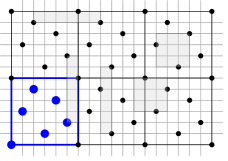
Figure 1: This non-lattice periodic grid point-set pierces all translates of $\mathcal{F}_{0}=\{6\times 1,1\times 6,3\times 3\}$.

3 Lattice piercing

Let $\mathcal{F}$ be a finite family of axis-parallel rectangles; denote by $A_{\min}$ the minimum area of a rectangle in $\mathcal{F}$. Let $\Lambda$ be an $\mathcal{F}$-piercing lattice and let $P$ be a fundamental parallelogram whose area is $A=\text{Area}(P)$. The following observation is in order:

Observation 1.

$A\leq A_{\min}$.

Two parameters of interest in a lattice are (see also [5, Ch. 4]):

• the smallest interpoint distance $\lambda$

• the distance $\mu$ between two consecutive parallel $\lambda$-lines. These are lattice lines of direction $u$, where the interpoint distance is $\lambda$; these lines are also referred to as $u$-lines.

Note that $A=\lambda\mu$. We start with a lemma of independent interest spelling out two inequalities between these parameters. (The second item is Theorem 1.3 in [8]. Nevertheless, we provide our own proof.)

Lemma 1.

The following inequalities hold:

1. $\lambda\leq\frac{2}{\sqrt{3}}\mu$

2. $\lambda\leq\sqrt{\frac{2A}{\sqrt{3}}}$

Proof.

Consider two consecutive parallel $\lambda$-lines $\ell_{1},\ell_{2}$ at distance $\mu$ from each other. Refer to Fig. 2.

Figure 2: Two consecutive parallel $\lambda$-lines.

Let $a,b\in\Lambda\cap\ell_{1}$ be consecutive lattice points on $\ell_{1}$ and $c\in\Lambda\cap\ell_{2}$ be a lattice point whose orthogonal projection $c^{\perp}$ onto $\ell_{1}$ lies between $a$ and $b$, and say, $|ca|\leq|cb|$. Consider the translation $T$ along $\ell_{2}$ that brings $c^{\perp}$ into the midpoint of $ab$. The result (obtained by extending the points on $\ell_{1}$ and $T(\ell_{2})$ to a lattice) is another lattice $T(\Lambda)$ with the same parameters $\lambda$ and $\mu$. The translation $T$ increases the minimum distance between $\Lambda\cap\ell_{1}$ and $T(\Lambda)\cap\ell_{2}$ to $\sqrt{\lambda^{2}/4+\mu^{2}}$, and so

$$\lambda\leq|ca|\leq\sqrt{\lambda^{2}/4+\mu^{2}},$$

or $\lambda\leq\frac{2\mu}{\sqrt{3}}$, proving the first inequality. Taking into account that $A=\lambda\mu$, we deduce $\lambda^{2}\leq\frac{2\lambda\mu}{\sqrt{3}}=\frac{2A}{\sqrt{3}}$, or $\lambda\leq\sqrt{\frac{2A}{\sqrt{3}}}$, proving the second inequality. ∎

Canonical vector basis.

We next argue about the existence of a canonical vector basis, i.e., one satisfying properties P1–P3 listed earlier in Section 1. Consider an $\mathcal{F}$-piercing lattice $\Lambda$ and a vector basis $\{u,v\}$, where $u$ is a shortest vector in $\Lambda$ ($|u|=\lambda$), and $v$ is chosen as in Lemma 2 below. We may assume without loss of generality (by switching the orientation of the $x$-axis) that $u$-lines have positive slope. We can then choose $v$ as the vector connecting the origin with a suitable lattice point on the next $u$-line just below the origin. Since $\mu\geq\frac{\sqrt{3}}{2}\lambda$ (by Lemma 1), it is easily seen that there is at least one lattice point in the $4$th quadrant on this line. Since $v$ connects lattice points on two consecutive $u$-lines it follows that $\{u,v\}$ is a vector basis in $\Lambda$. In this lattice $u$ has positive (or $\infty$) slope and is a shortest vector, and $v$ has negative (or $0$) slope, i.e., $u=[a,b]$, $v=[c,-d]$ with $a,b,c,d\geq 0$ and $b>0$. In particular, any pair of points in the lattice can be connected by $2$-edge polygonal path along directions $u$ and $v$: we refer to such a path as $uv$-path.

Let $0<\alpha<180^{\circ}$ be the angle made by $u$ and $v$. Our construction will ensure that $45^{\circ}\leq\alpha\leq 135^{\circ}$. The property that $\alpha$ is not to far from $90^{\circ}$ is key in bounding from above the complexity (and length) of a path connecting any two points in the lattice along directions $u$ and $v$. (See also [12, Ch. 27] for a similar angle property of the shortest vector derived from different principles.)

Let $\ell$ be a $u$-line through the origin with a positive slope and $\ell^{\prime}$ be the next $u$-line below $\ell$, where $|u|=\lambda$; $\ell$ and $\ell^{\prime}$ are parallel lattice lines. (The case when $\ell$ and $\ell^{\prime}$ are vertical is an easy special case omitted from the proofs.)

Lemma 2.

There exists a vector basis $[u,v]$ so that $u$ is a shortest vector and $u$ has positive (or $\infty$) slope, $v$ has negative (or $0$) slope , and the angle $\alpha$ made by $u$ and $v$ satisfies $45^{\circ}\leq\alpha\leq 135^{\circ}$. This interval is the best possible; i.e., it is minimal with respect to inclusion. Moreover, $|v|^{2}\leq\lambda^{2}+\mu^{2}$.

Proof.

We will choose $v$ such that its endpoint lies on $\ell^{\prime}$. Refer to Fig. 3 (left) for the following notations. Let $A$ be the endpoint of $u$ and let $p$ denote the orthogonal projection of $O$ onto $\ell^{\prime}$. Finally, denote by $B_{0}$ the rightmost lattice point on $\ell^{\prime}$ that lies in the third quadrant and denote by $B_{i}=B_{0}+i\cdot u$ the following lattice points along the line $\ell^{\prime}$. In particular, let $B_{l}$ the last lattice point on $\ell^{\prime}$ in the fourth quadrant ($l\geq 1$); it can be easily seen that the set of points $B_{i}$, $i\geq 1$ in the $4$th quadrant is nonempty.

Figure 3: The angle between $u$ and $v$ is mid-range (i.e., not too acute or too obtuse).

We distinguish two cases:

Case 1: the slope of $\ell$ is at most $1$. Refer to Fig. 3 (middle). We will set $v:=OB_{i}$ for a suitable $i\geq 1$. Initially set $v:=OB_{1}$. Since $B_{1}A$ has positive slope, we have $\beta\leq 90^{\circ}$, whence $\alpha+\gamma\geq 90^{\circ}$. In $\triangle OB_{1}A$ the side $OA$ is the shortest one, hence the corresponding angle $\gamma$ is the smallest one. In particular $\gamma\leq\alpha$ hence $\alpha\geq 45^{\circ}$. By the case distinction we also have $\alpha\leq 135^{\circ}$, as required.

We next choose a suitable $i\geq 1$ so that $v:=OB_{i}$ satisfies the upper bound on length while the angle interval is maintained. Let $i\geq 0$ be the maximum integer so that $B_{i}$ is left of $p$ on $\ell^{\prime}$. If $i=0$, we keep the original setting $v:=OB_{1}$ and see that the inequality $|v|^{2}=OB_{1}^{2}=\mu^{2}+pB_{1}^{2}\leq\mu^{2}+\lambda^{2}$ is clearly verified. If $i\geq 1$, $\alpha\geq 90^{\circ}$ and we reset $v:=OB_{i}$. This new setting decreases $\alpha$, however $\alpha\geq 90^{\circ}$ remains valid by construction, whence $\alpha\geq 45^{\circ}$ still holds. In the latter case we have $|v|^{2}=OB_{i}^{2}=\mu^{2}+pB_{i}^{2}\leq\mu^{2}+\lambda^{2}$, as required.

Case 2: the slope of $\ell$ is at least $1$. Refer to Fig. 3 (right). We will set $v:=OB_{i}$ for a suitable $i\geq 1$. Initially set $v:=OB_{l}$. Note that $\beta+\gamma$ equals the measure of the exterior angle $\angle COB_{l+1}$ in $\triangle OB_{l+1}A$ corresponding to $O$. By construction (the definitions of $B_{0}$ and $B_{l+1}$), this angle is at least $90^{\circ}$, hence $\beta+\gamma\geq 90^{\circ}$. In $\triangle OB_{l+1}A$ the side $OA$ is the shortest one, hence the corresponding angle $\gamma$ is the smallest one. In particular $\gamma\leq\beta$ hence $\beta\geq 45^{\circ}$ or $\alpha\leq 135^{\circ}$ (as complementary angles). By the case distinction we also have $\alpha\geq 45^{\circ}$, as required.

We next choose a suitable $i\geq 1$ so that $v:=OB_{i}$ satisfies the upper bound on length while the angle interval is maintained. Let $i\geq 0$ be the minimum integer so that $B_{i}$ is right of $p$ on $\ell^{\prime}$. If $i=l+1$, we keep the original setting $v:=OB_{l}$ and see that the inequality $|v|^{2}=OB_{l}^{2}=\mu^{2}+pB_{l}^{2}\leq\mu^{2}+\lambda^{2}$ is clearly verified. If $i\leq l$, $\alpha\leq 90^{\circ}$ and we reset $v:=OB_{i}$. This new setting increases $\alpha$, however $\alpha\leq 90^{\circ}$ remains valid by construction, whence $\alpha\leq 135^{\circ}$ still holds. In the latter case we have $|v|^{2}=OB_{i}^{2}=\mu^{2}+pB_{i}^{2}\leq\mu^{2}+\lambda^{2}$, as required.

Figure 4: Tight cases of optimality.

To verify the optimality of the angles $45^{\circ}$ and $135^{\circ}$ consider two lattices obtained from the integer lattice $\mathbb{Z}^{2}$ by a small perturbation consisting of suitable scaling and clockwise rotation. See Fig. 4. ∎

Lemma 3.

Let $\Lambda$ be an optimal $\mathcal{F}$-piercing lattice with density $1/A$, and let $\{u,v\}$ be a vector basis of $\Lambda$, where $\lambda=|u|$ is the smallest interpoint distance in $\Lambda$ and $v$ is chosen as in the above construction. Then $1/2\leq|u|\leq|v|\leq\sqrt{\frac{7}{3}}\,\frac{A}{\lambda}$.

Proof.

We first show that $\lambda\geq 1/2$. Assume for contradiction that $\lambda<1/2$. Recall that (i) $A=\lambda\mu\geq 1$ (since the integer lattice $\mathbb{Z}^{2}$ is $\mathcal{F}$-piercing), and so $\mu>2$; and (ii) the minimum rectangle width and height in $\mathcal{F}$ are $1$. Let $\theta>0$ denote the angle made by a $u$-line $\ell$ with the $x$-axis. Consider a new lattice $\Lambda^{\prime}$ with basis $(u^{\prime},v^{\prime})$ derived from $\Lambda$ by making the following replacements that keep every other lattice point on each $u$-line (for each line, one of the two possible choices is made arbitrarily):

$$\begin{cases}\lambda\to\lambda^{\prime}:=2\lambda\\ \mu\to\mu^{\prime}:=\frac{\mu+\varepsilon}{2}\end{cases}$$ (1)

where $\varepsilon>0$ is sufficiently small; in particular, $\varepsilon<\mu-2$. That is: $u^{\prime}=2u$ and the distance between $u$-lines is almost cut in half by new lattice lines bisecting the respective parallel strips. The lattice points on the new lines are the midpoints of shortest interpoint connecting segments. We have $|u^{\prime}|<1$ and $\mu^{\prime}>1$. See Fig. 5. We next verify that $\Lambda^{\prime}$ is still an $\mathcal{F}$-piercing lattice.

Figure 5: Obtaining $\Lambda^{\prime}$ from $\Lambda$. Left: a maximal empty rectangle amidst the points of $\Lambda$. Right: a translate of this rectangle is pierced by a lattice point on the lattice line bisecting the parallel strip.

Let $R$ be an arbitrary maximal empty rectangle amidst the points in $\Lambda$ that is determined by two adjacent $u$-lines $\ell_{1}$ and $\ell_{2}$ (i.e., $R$ is incident to two points on each of the two lines). Let $\ell$ denote the line bisecting the parallel strip made by $\ell_{1}$ and $\ell_{2}$; denote by $\ell^{\prime},\ell^{\prime}_{1},\ell^{\prime}_{2}$ the corresponding replacement lines in $\Lambda^{\prime}$. Let $R^{\prime}$ be a translate of $R$ empty of lattice points in $\ell^{\prime}_{1}$ and $\ell^{\prime}_{2}$ whose center lies in this parallel strip. We next show that $\Lambda^{\prime}$ pierces $R^{\prime}$. Observe that $|R\cap\ell_{1}|=|R\cap\ell_{2}|=\lambda$, and $|R^{\prime}\cap\ell_{1}|,|R^{\prime}\cap\ell_{2}|\leq 2\lambda$. After the replacement $\Lambda\to\Lambda^{\prime}$, we can no longer guarantee that $R^{\prime}$ intersects both $\ell^{\prime}_{1}$ and $\ell^{\prime}_{2}$; however, if $R^{\prime}$ does not intersect, say, $\ell^{\prime}_{i}$, then the corresponding corner of $R^{\prime}$ is at distance at most $\varepsilon$ from it. In addition, we have $|R^{\prime}\cap\ell^{\prime}_{1}|,|R^{\prime}\cap\ell^{\prime}_{2}|\leq 2\lambda$.

To prove our claim that $\Lambda^{\prime}$ pierces $R^{\prime}$ we distinguish two cases.

Case 1: $\ell^{\prime}$ intersects $R^{\prime}$ in two opposite sides. Then $|\ell\cap R^{\prime}|\geq 1>2\lambda$, and so $R^{\prime}$ is pierced by a lattice point on $\ell^{\prime}$.

Case 2: $\ell^{\prime}$ intersects $R^{\prime}$ in two adjacent sides; we may assume without loss of generality that $\ell^{\prime}$ intersects the left and top side of $R^{\prime}$. Suppose first that $\theta\leq 45^{\circ}$. Let $y$ be the length of the orthogonal projection from the upper-left corner of $R^{\prime}$ to $\ell^{\prime}$. The intersection $R^{\prime}\cap\ell^{\prime}$ is partitioned into two segments of lengths $s_{1}$ and $s_{2}$, where $s=s_{1}+s_{2}$. Then $\tan\theta=\frac{y}{s_{2}}$, hence by construction we have

$$s_{2}=\frac{y}{\tan\theta}\geq y\geq\frac{\mu+\varepsilon}{2}-\varepsilon=\frac{\mu-\varepsilon}{2}>1.$$

It follows that $|\ell^{\prime}\cap R^{\prime}|\geq s>s_{2}>1>2\lambda$, and so $R^{\prime}$ is pierced by a lattice point on $\ell^{\prime}$. When $\theta\geq 45^{\circ}$, a similar argument yields $|\ell^{\prime}\cap R^{\prime}|\geq s>s_{1}>1>2\lambda$, and the same conclusion holds.

In both cases we have shown that $\Lambda^{\prime}$ pierces $R^{\prime}$. However, the area of the fundamental parallelogram of $\Lambda^{\prime}$ is $A^{\prime}=\lambda^{\prime}\mu^{\prime}=2\lambda\cdot\frac{\mu+\varepsilon}{2}>\lambda\mu=A$, contradicting the optimality of $\Lambda$. It follows that the initial assumption $\lambda<1/2$ was false and we must have $\lambda\geq 1/2$.

We next show that $|v|\leq\sqrt{\frac{7}{3}}\,\frac{A}{\lambda}$. Recall that $A=\lambda\mu$ and that $\lambda\leq\frac{2\mu}{\sqrt{3}}$ (by the first inequality of Lemma 1). Observe that $|v|$ cannot be much longer than $\mu$. Indeed, by the second inequality of Lemma 2, we have

$$|v|\leq\sqrt{\mu^{2}+\lambda^{2}}\leq\sqrt{\mu^{2}+\frac{4\mu^{2}}{3}}=\sqrt{\frac{7}{3}}\,\mu=\sqrt{\frac{7}{3}}\,\frac{A}{\lambda}.\qed$$

In summary, for any finite family $\mathcal{F}$ of axis-parallel rectangles of dimensions at least $1$, there is an optimal $\mathcal{F}$-piercing lattice $\Lambda$ with a canonical vector basis $\{u,v\}$ satisfying properties P1–P3 given in the introduction.

4 A decision algorithm (proof of Theorem 1)

Suppose in what follows that the premises of Theorem 1 are satisfied. Since the lattice is periodic, it suffices to consider (i) rectangles whose left sides contain the origin and (ii) rectangles whose lower sides contain the origin. Indeed, if $R$ is a maximal empty rectangle amidst the points of the lattice, there is a congruent maximal empty rectangle $R^{\prime}$ supported on the left or from below by the origin. The latter case appears when the lattice contains horizontal lattice lines (i.e., there exist lattice points with the same $y$-coordinate); and can be easily dealt with by examining the distance between consecutive horizontal lattice lines. We call such rectangles supported (by the origin, on the left or from below). Moreover, since each side of each rectangle is at most $k$, we can restrict our attention to lattice points contained in a board rectangle $D=[0,k]\times[-k,k]$. Let $N=\mathcal{O}(k^{2}/A)$ be the number of lattice points $i\cdot u+j\cdot v$, $i,j\in\mathbb{Z}$, contained in $D$. In particular, for each lattice point in $D$ we have $|i|=\mathcal{O}(k/\lambda)=\mathcal{O}(k)$ and $|j|=\mathcal{O}(k/A)$ by Lemma 3.

The decision algorithm proceeds in two steps: First, find all maximal supported rectangles that are contained in $D$. Second, check if any of those rectangles is coordinate-wise larger than any rectangle in $\mathcal{F}$. If not, output that the lattice $\Lambda$ is $\mathcal{F}$-piercing.

For the first step, construct the set of lattice points $P=\{p\in D\}$ such that the rectangle with diagonal $op$ is empty. It turns out that this set has a special structure as described in the following.

Lemma 4.

There are $\mathcal{O}(k)$ maximal empty rectangles supported by the origin on the left side and all can be found in $\mathcal{O}(k\log{k})$ time.

Proof.

Let $P$ be the set of lattice points $p\in D$ such that $R(o,p)$ is empty. Here $R(o,p)$ denotes the rectangle determined by $o$ and $p$. Let $P=P^{+}\cup P^{-}$ be the partition of $P$ induced by the $x$-axis ($P^{+}$ and $P^{-}$ are the points above and respectively below the $x$-axis, with ties broken arbitrarily.) Order $P^{+}$ and $P^{-}$ by $x$-coordinate and observe that: (i) $P^{+}$ must form a sequence of points with decreasing $y$-coordinates; and (ii) $P^{-}$ must form a sequence of points with increasing $y$-coordinates. We refer to $P=P^{+}\cup P^{-}$ as the funnel, where $P^{+}$ is the upper funnel and $P^{+}$ is the lower funnel. Recall that the sides of $D$ have length $\mathcal{O}(k)$. Since $\lambda\geq 1/2$ is the smallest interpoint distance, we have $|P^{+}|,|P^{-}|=\mathcal{O}(k)$, whence $|P|=\mathcal{O}(k)$. ∎

Generating the funnel.

Recall that $u$ lies in the first quadrant and $v$ in the fourth quadrant. For a fixed $j\in\mathbb{Z}$, let $\ell_{j}$ be the lattice consisting of the lattice points $L(i,j):=i\cdot u+j\cdot v$, with $i\in\mathbb{Z}$. Given $j$, first a closed interval $J=[j_{1},j_{2}]$ is determined so that $\ell_{j}\cap D$ is non-empty whenever $j\in J$; note that $0\in J$. A binary search procedure accomplishes this task in $\mathcal{O}(\log{k})$ time. Since $u\in\ell_{0}$ yields the shortest interpoint distance in $\Lambda$, we have $u\in P^{+}$ and no other lattice point on $\ell_{0}$ belongs to $P$. We process the other $u$-lines $\ell_{j}$ one by one: the lines above $\ell_{0}$ are processed in decreasing order of $j$; the lines below $\ell_{0}$ are processed in increasing order of $j$. When processing the lines above $\ell$, we compute the point with smallest non-negative $x$-coordinate and we include it to $P^{+}$ if the point belongs to $D$ and its $x$-coordinate is less than all the $x$-coordinates of the points already processed (again, these points can computed by binary search). These points of $P^{+}$ form a branch starting at $u$ and approaching the positive part of the $y$-axis. Similarly, we add to $P^{+}$ the points that form a branch starting at $u$ and approaching the positive part of the $x$-axis; these points are obtained by processing the lines below $\ell$. The points in $P^{+}$ (the union of two branches) are then sorted by their $x$-coordinates, as they form the upper funnel. Refer to Fig. 6.

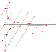
Figure 6: A maximal empty rectangle amidst the points of the funnel; the rectangle is supported from the left by the origin.

The computation of the lower funnel is analogous to the computation of the upper funnel. As before, we construct two branches, this time approaching the positive part of the $x$-axis and the negative part of the $y$ axis. The points in $P^{-}$ are then sorted by their $x$-coordinates, as they form the lower funnel.

We stop generating a branch at one point once any of those occur: (i) the $u$-line is ”too far” (it no longer intersects the board) or (ii) we get a point on the axis (if it is on the $x$-axis, put it into the bottom branch) or (iii) the distance of the champion to the respective axis is below $1$ (for the current rightmost point in $P^{+}$ and the $x$-axis, the current rightmost point in $P^{-}$ and the $x$-axis, the current highest point in $P^{+}$ and the $y$-axis, or the current lowest point in $P^{-}$ and the $x$-axis). Case (iii) is optional.

Decision algorithm and its complexity.

Since $A\geq 1$ and $|v|\geq|u|\geq 1/2$, we have $|v|=\Omega(1)$, thus only $\mathcal{O}(k)$ lines are to be processed. For each processed $u$-line, the required computation takes $\mathcal{O}(\log{k})$ time. Each line contributes $\mathcal{O}(1)$ points to the funnel $P$. Together with the sorting the first step takes $\mathcal{O}(k\log k)$ time and the produced set $P$ has size $\mathcal{O}(k)$.

For the second step, consider each rectangle in $R\in\mathcal{F}$ one by one. The funnel structure is binary searched by the rectangle width $w$ and the corresponding implied height is obtained from the funnel structure. The necessary decision is immediately taken based on the rectangle height $h$. There are $n$ rectangles in $\mathcal{F}$ and it takes $\mathcal{O}(\log{k})$ time to process each of them. The resulting time for the second step is $\mathcal{O}(n\log k)$.

The overall complexity of the decision algorithm is thus $\mathcal{O}(k\log k+n\log k)=\mathcal{O}((k+n)\log{k})$.

5 Computing an optimal $\mathcal{F}$-piercing lattice

We present two pseudo-polynomial time algorithms for finding the optimal piercing density for a set of $n$ axis-parallel rectangles: their running time are polynomial in the number of rectangles and the maximum aspect ratio of the rectangles in the family. (See [9, Ch. 9] for basic technical terms regarding algorithm complexity.) The second algorithm assumes that the rectangles have integer side-lengths.

5.1 Preliminaries

By properties P1–P3, the area of a fundamental parallelogram of $\Lambda$ is $A=ab+cd>0$. As such, $A$ is an increasing function in each of the four variables.

An $\mathcal{F}$-piercing lattice $\Lambda$ is said to be $x$-tight with respect to $\mathcal{F}$ if there exist (not necessarily distinct) rectangles $R_{s},R_{t}\in\mathcal{F}$ such that for some $i_{s},j_{s},i_{t},j_{t}\in\mathbb{Z}$ we have

$$i_{s}\cdot a+j_{s}\cdot c =w_{s},$$

$$i_{t}\cdot a+j_{t}\cdot c =w_{t},$$

where both constraints are linearly independent (the determinant of the linear system in $a,c$ is nonzero). Note that each equation has at least one positive term, i.e., $\max(i_{s},j_{s})\geq 1$ and $\max(i_{i},j_{t})\geq 1$.

An $\mathcal{F}$-piercing lattice $\Lambda$ is said to be $y$-tight with respect to $\mathcal{F}$ if there exist (not necessarily distinct) rectangles $R_{s},R_{t}\in\mathcal{F}$ such that for some $i_{s},j_{s},i_{t},j_{t}\in\mathbb{Z}$ we have

$$i_{s}\cdot b+j_{s}\cdot d =h_{s},$$

$$i_{t}\cdot b+j_{t}\cdot d =h_{t},$$

where both constraints are linearly independent. Similarly each equation has at least one positive term.

An $\mathcal{F}$-piercing lattice $\Lambda$ is said to be tight with respect to $\mathcal{F}$ (or $\mathcal{F}$-tight) if $\Lambda$ is $x$-tight with respect to $\mathcal{F}$ and $y$-tight with respect to $\mathcal{F}$. The key to both algorithms is the following.

Lemma 5.

Let $\Lambda$ be an $\mathcal{F}$-piercing lattice with minimum density. Then $\Lambda$ is $\mathcal{F}$-tight.

Proof.

Consider the set of maximal rectangles of width and height at least $1$ supported from the left or from below by the origin. Since every such maximal rectangle is contained in $D$, this set is finite. For each such rectangle $R=w^{\prime}\times h^{\prime}$, and for each input rectangle $R_{i}$, $i=1,\ldots,n$, the piercing condition requires

$$w^{\prime}\leq w_{i}\text{ or }h^{\prime}\leq h_{i}.$$ (2)

Observe that each constraint of the form $w^{\prime}\leq w_{i}$ can be expressed as a linear inequality in $a,c$, whereas each constraint of the form $h^{\prime}\leq h_{i}$ can be expressed as a linear inequality in $b,d$. Indeed, since the points that support $R$ are lattice points, $w^{\prime}$ can be expressed as an integer combination of $a$ and $c$, and $h^{\prime}$ can be expressed as an integer combination of $b$ and $d$. Construct a finite system $\Psi$ of linear inequalities by putting in $\Psi$ every inequality of this type. Let $g_{ac}\leq 2$ and $g_{bd}\leq 2$ be the number of independent $x$-tight inequalities (equations), and respectively $y$-tight inequalities that can be extracted from the system. Next we show that $g_{ac}=g_{bd}=2$ in a proof by contradiction.

If $g_{ac}=0$, pick a variable ($a$ or $c$) that appears with a positive coefficient in at least one inequality in $\Psi$ and increase it (i.e., continuously modify $\Lambda$) by a small $\varepsilon>0$ (during which interval the system of inequalities describing the lattice constraints on the rectangles does not change). Since the piercing condition is maintained and $A$ increases, this contradicts the optimality of $\Lambda$. Therefore $g_{ac}\geq 1$. By a symmetric argument we also have $g_{bd}\geq 1$.

If one of $g_{ac},g_{bd}$ is $1$ and the other one is $2$, we may assume without loss of generality that $g_{ac}=1$ and $g_{bd}=2$. This means that $b,d\geq 0$ are determined (i.e., constants). Since $g_{ac}=1$, the area $A=ad+bc$ is a linear function in one variable ($a$ or $c$), say, $A=\ell(a)$ for some $a>0$. Then every remaining inequality in $\Psi$ is linear in $a$. Depending on the sign of the coefficient of $a$, increase or decrease $a$ (i.e., continuously modify $\Lambda$) by a small $\varepsilon>0$ such that $A$ increases. Since $g_{ac}=1$ and $\varepsilon>0$ is small, the inequalities defining the rectangles do not switch. Since the piercing condition is maintained and $A$ increases, this contradicts the optimality of $\Lambda$.

The last case to consider is $g_{ac}=g_{bd}=1$. Then the area expression $A=ad+bc$ becomes a function of two variables (one from $\{a,c\}$ and one from $\{b,d\}$), say, $A=ad+bc=r_{1}ab+r_{2}a+r_{3}b$, where $r_{1},r_{2},r_{3}\in\mathbb{R}$. In addition, there exist $a,b>0$ such that $f(a,b):=r_{1}ab+r_{2}a+r_{3}b>0$. It suffices to show that $f(a,b)$ has no local maximum for $a,b>0$. If $r_{1}=0$, this is obvious since $f(a,b)$ is then a linear function in $a$ and $b$, and a suitable small change in one of the variables leads to an increase in $A=f(a,b)$, contradicting the optimality of $\Lambda$. If $r_{1}\neq 0$, write

$$f_{a}:=\frac{\partial f}{\partial a},\ \ f_{b}:=\frac{\partial f}{\partial b},\ \ f_{aa}:=\frac{\partial^{2}f}{\partial a^{2}},\ \ f_{bb}:=\frac{\partial^{2}f}{\partial b^{2}},\ \ f_{ab}:=\frac{\partial^{2}f}{\partial b\partial a}\text{ or }\frac{\partial^{2}f}{\partial a\partial b},$$

and let $\Delta:=f_{aa}f_{bb}-(f_{ab})^{2}$. By a well known theorem in calculus (see, e.g., [11, Thm. 22.15]), if $\Delta<0$ at $(a,b)$, then $(a,b)$ is not a local maximum (nor a local minimum). We verify that $f_{aa}=f_{bb}=0$ and $f_{ab}=r_{1}$, thus $\Delta=f_{aa}f_{bb}-(f_{ab})^{2}=-r_{1}^{2}<0$ and so $f(a,b)$ has no local maxima for $a,b>0$. As such, a suitable small change in one of the variables leads to an increase in $A=f(a,b)$, contradicting the optimality of $\Lambda$.

Consequently, the only remaining case is $g_{ac}=g_{bd}=2$, as required. ∎

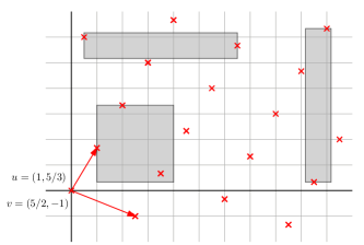
Figure 7: This lattice pierces all translates of rectangles in $\mathcal{F}_{0}=\{6\times 1,1\times 6,3\times 3\}$.

Lemma 5 immediately yields the following.

Corollary 1.

When all rectangles have rational side-lengths there is an optimal lattice with a rational vector basis.

Example.

An extremal (i.e., optimal) lattice $\Lambda$ corresponds to a pair of $2\times 2$ linear systems, one in the variables $a,c$ and one in the variables $b,d$. Consider the lattice in Fig. 7. This lattice corresponds to the systems below. Indeed, their solutions are $a=1$, $c=5/2$, and $b=5/3$, $d=1$. Note that the above solution also satisfies the inequality $b+d\leq 3$ (relevant for the piercing of $3\times 3$ rectangles).

$$\begin{aligned} \begin{cases}a=1\\ a+2c=6\end{cases}\end{aligned}\hskip 85.35826pt\begin{aligned} \begin{cases}d=1\\ 3b+d=6\end{cases}\end{aligned}$$

5.2 The first algorithm

By Lemma 5, an $\mathcal{F}$-piercing lattice of optimal density is tight. Therefore, it suffices to generate all tight lattices and output a lattice that is $\mathcal{F}$-piercing and has minimum density (i.e., largest area $A$). The algorithm essentially guesses the optimal lattice by exhaustive enumeration of all lattices that are tight with respect to $\mathcal{F}$ and have density in a prescribed interval. It retains those that are $\mathcal{F}$-piercing and finally returns one with optimal density.

For guessing the four tight inequality constraints, it suffices to choose two lattice points $p_{1},p_{2}\in D$ so that the point pairs $o,p_{1}$ and $o,p_{2}$ correspond to the two $x$-constraints and four lattice points $p_{3},p_{4},p_{5},p_{6}\in D$ so that the point pairs $p_{3},p_{4}$ and $p_{5},p_{6}$ correspond to the two $y$-constraints (not all six points need to be distinct). One can draw a constraint graph on the lattice points by including these point pairs; an example appears in Fig. 8.

Recall that $D$ is the board rectangle of diameter $\mathcal{O}(k)$. Since $p_{3},p_{4}$ are lattice points, $p_{3}p_{4}=op^{\prime}_{3}$ for a suitable lattice point $p^{\prime}_{3}\in D$. Similarly, $p_{5}p_{6}=op^{\prime}_{4}$ for a suitable lattice point $p^{\prime}_{4}\in D$. Here choosing a lattice point means specifying the integers $i,j$ for the lattice point $L(i,j):=i\cdot u+j\cdot v$. It is worth noting that this choice is symbolical in the sense that the vectors $u,v$ are left unspecified. By Lemma 2, any pair of lattice points $p,q\in D$ can be connected by a $2$-edge polygonal path along directions $u$ and $v$ and whose length is $\mathcal{O}(k)$. Moreover, since $\lambda=\Omega(1)$ (by Lemma 3), if $pq=i\cdot u+j\cdot v$, then $|i|+|j|=\mathcal{O}(k)$. In summary, guessing one constraint is equivalent to choosing $i$ and $j$ as above and this can be done in $\mathcal{O}(N)=\mathcal{O}(k^{2})$ ways. Recall that $N=\mathcal{O}(k^{2}/A)$ is the number of lattice points $i\cdot u+j\cdot v$, $i,j\in\mathbb{Z}$ contained in $D$. (This argument is applied once again in Sections 8 and 9 with extra care for obtaining sharper numeric bounds for the specific rectangle family considered there.)

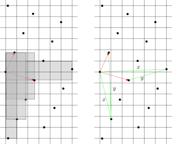
Figure 8: A (slightly suboptimal) lattice $\Lambda$ for $\mathcal{F}=\{6\times 1,1\times 6,3\times 3\}$ with vector basis $u=(4/5,7/4)$, $v=(13/5,-3/4)$ and area $A=103/20$. There are four maximal empty rectangles whose dimensions are at least $1$ that are supported on the left by the origin. The four green edges in the constraint graph (two $x$-edges and two $y$-edges) are given by three of these rectangles. Each constraint is a linear equation in two variables.

For each tuple of at most four points $p_{1},p_{2},p^{\prime}_{3},p^{\prime}_{4}$ as described above, there are $\mathcal{O}(1)$ ways to group them into pairs and generate two $x$-constraints (in variables $a,c$) and two $y$-constraints (in variables $b,d$). For each such combination, the two linear systems are solved and the corresponding lattice $\Lambda=\Lambda(a,b,c,d)$ with vectors $u=(a,b)$ and $v=(c,-d)$ is “generated” as explained below provided that properties P1–P3 are satisfied.

Denote by $A_{\min}$ the minimum area of a rectangle in $\mathcal{F}$ and by $A_{\textsf{OPT}}$ the area of the fundamental parallelogram of an optimal $\mathcal{F}$-piercing lattice ($1\leq A_{\min}\leq k^{2}$). Recall that a lattice with density $1/A^{\prime}$ can be computed in $\mathcal{O}(n)$ time [4], where $A^{\prime}$ satisfies (for convenience we replaced the $1.895$-ratio from Theorem 8 by $2$):

$$\frac{A_{\min}}{2}\leq A^{\prime}\leq A_{\min}.$$ (3)

Recall that $D$ contains $N$ lattice points. There are $\mathcal{O}(N^{4})$ ways to choose a tuple of at most four points out of $N$, and for each of them, at most $\mathcal{O}(n^{4})$ ways to “match” them with at most four rectangles out of the given $n$ rectangles in $\mathcal{F}$. Consequently, there are $\mathcal{O}(N^{4}n^{4})$ candidate lattices for the $\mathcal{F}$-piercing test to be generated; a lattice is immediately discarded if its area $A$ satisfies: $A<A^{\prime}$, according to (3).

For each lattice $\Lambda$ satisfying suitable conditions (as imposed by P1–P3) the decision algorithm from Section 4 determines if $\Lambda$ is $\mathcal{F}$-piercing. Since its running time is $\mathcal{O}((k+n)\log{k})$ time, and $N=\mathcal{O}(k^{2}/A)=\mathcal{O}(k^{2})$, the overall running time becomes

$$\mathcal{O}\left((N^{4}n^{4})(k+n)\log{k}\right)=O\left(k^{8}n^{4}(k+n)\log{k}\right).$$

6 The second algorithm

The algorithm works on input families whose rectangles have integer side-lengths. The general scheme is the same as in the first algorithm. However, instead of generating and solving all linear systems that are tight with respect to $\mathcal{F}$, two integer upper bounds $M_{ac}$ and $M_{bd}$ are deduced such that the algorithm considers only lattices whose vectors $u=(a,b)$, $v=(c,-d)$, where $a,c$ are positive fractions with common denominator $M_{ac}$ and $b,d$ are positive fractions with common denominator $M_{bd}$. $M_{ac}$ is a valid upper bound on the absolute value of a $2\times 2$ determinant of the linear system in $a,c$. Similarly, $M_{bd}$ is a valid upper bound on the absolute value of a $2\times 2$ determinant of the linear system in $b,d$. For the reference, ideas of a similar nature and an application appear in [10].

For each of the two linear systems, each coefficient is an integer of size $\mathcal{O}(k)$. As such, each $2\times 2$ the absolute value of each determinant is $\mathcal{O}(k^{2})$ and so the solutions of the linear systems are rational tuples $(a,c)$ and $(b,d)$ with denominators $\mathcal{O}(k^{2})$. The algorithm tries all possible combinations $M_{ac}=1,2,\ldots,\mathcal{O}(k^{2})$, $M_{bd}=1,2,\ldots,\mathcal{O}(k^{2})$ without solving any linear system. For each combination, it generates all possible vector bases whose coordinates have these denominators (as explained below). For each vector basis and corresponding lattice $\Lambda$, the algorithm verifies whether $\Lambda$ is $\mathcal{F}$-piercing and if so, it computes its density.

Let ${\rm Num}(f)$ and ${\rm Den}(f)$ denote the numerator and denominator of a fraction $f$. For a fixed $M_{ac}$ and $M_{bd}$, there are $\mathcal{O}(\sqrt{A}k^{2})$ choices for ${\rm Num}(a)$ and $\mathcal{O}(\sqrt{A}k^{2})$ choices for ${\rm Num}(b)$ (since $|u|\leq|v|$ and $|u||v|\leq 2A$); and $\mathcal{O}(Ak^{2})$ choices for ${\rm Num}(c)$ and $\mathcal{O}(Ak^{2})$ choices for ${\rm Num}(d)$. Summing up over all $M_{ac}=1,2,\ldots,\mathcal{O}(k^{2})$ and $M_{bd}=1,2,\ldots,\mathcal{O}(k^{2})$ yields $\mathcal{O}(k^{4})$ choices for $M_{ac}$ and $M_{bd}$, and for each such choice $\mathcal{O}(A^{3}k^{8})$ choices for the numerators of $a,b,c,d$.

Every combination yields a candidate lattice for the $\mathcal{F}$-piercing test, whence there are $\mathcal{O}(A^{3}k^{12})$ lattices to be verified. Since the running time of the decision algorithm is $\mathcal{O}((k+n)\log{k})$, and $A=\mathcal{O}(k^{2})$, the overall running time becomes

$$\mathcal{O}\left(A^{3}k^{12}(k+n)\log{k}\right)=\mathcal{O}\left(k^{18}(k+n)\log{k}\right).$$

7 A preliminary separation result

Proof of Theorem 4.

Let $\mathcal{F}_{0}=\{6\times 1,1\times 6,3\times 3\}$. Assume for contradiction that $\pi_{L}(\mathcal{F}_{0})\leq 1/6+\varepsilon$, for some small $\varepsilon>0$: The value $\varepsilon=3\cdot 10^{-7}$ will be shown to work. Let $\Lambda$ be an $\mathcal{F}_{0}$-piercing lattice. Let $P$ be a fundamental parallelogram of $\Lambda$ and $A=\text{Area}(P)$. It follows that $6-\delta\leq A\leq 6$, where $\delta=10^{-5}$. We first show that the diameter of $P$ is bounded from above by a constant.

Claim 1.

Let $P$ be a fundamental parallelogram of $\Lambda$, so that $P$ is determined by two consecutive $\lambda$-lines and has minimum diameter, say $D$. Then $\lambda\leq 2\cdot 3^{1/4}$ and $D<6$.

Proof.

Consider two adjacent parallel $\lambda$-lines $\ell_{1},\ell_{2}$ at distance $\mu$. Since $P$ has minimum diameter among all parallelograms determined by these two lines, we have $D\leq\sqrt{d^{2}+(3\lambda/2)^{2}}$. If $\mu>3\sqrt{2}$, the strip contains an unpierced $3\times 3$ square, contradicting the fact that $\Lambda$ is $\mathcal{F}_{0}$-piercing. Thus $\mu\leq 3\sqrt{2}$. By Lemma 1 we have $\lambda\leq\sqrt{\frac{2A}{\sqrt{3}}}\leq 2\cdot 3^{1/4}$. The two inequalities yield $D^{2}\leq 18+9\sqrt{3}<34$, or $D<6$, as claimed. ∎

Consider an axis-parallel square $Q$ of side-length $1800k$, where $k$ is a large positive integer. It will be convenient to think of $Q$ as being made from $k^{2}$ smaller squares (called here blocks). Each block $B$ is an axis-aligned square of side-length $1800$. Further, it will be convenient to think of each block as being made from $300^{2}=90000$ smaller squares (called here squares). Each square $S$ is an axis-aligned square of side-length $6$. By slightly translating $Q$ if needed, it may be assumed that no point in $\Lambda\cap Q$ is at integer distance from any side of $Q$ (equivalently, if $Q$ is partitioned by grid lines into unit squares, no point in $\Lambda$ lies on a grid line or on $Q$’s boundary.)

Claim 2.

$Q$ contains at most $540000.9k^{2}+\mathcal{O}(k)$ points in $\Lambda$.

Proof.

Note that $\text{Area}(Q)=(1800k)^{2}$. By 1 the number of lattice cells intersecting the boundary $\partial Q$ is $\mathcal{O}(k)$. It follows that $Q$ contains

$$\frac{\text{Area}(Q)}{\text{Area}(P)}+\mathcal{O}(k)\leq\frac{(1800k)^{2}}{6-\delta}+\mathcal{O}(k)\leq 540000.9k^{2}+\mathcal{O}(k)$$

points in $\Lambda$ provided that $\delta>0$ is sufficiently small ($\delta\leq 10^{-5}$ will suffice). ∎

Claim 3.

There is a block containing at most $6\cdot 9\cdot 10^{4}=540000$ points in $\Lambda$.

Proof.

Assume not, i.e., every block contains at least $540001$ points in $\Lambda$. Since $Q$ consists of $k^{2}$ blocks, it must contain at least $540001k^{2}$ points in $\Lambda$, contradicting 2 (for $k$ large enough). ∎

Let now $B$ denote such a block. In the remainder of the proof we will only work with $B$ (and no other block). Recall that $B$ contains exactly $300^{2}=90000$ squares (each square is $6\times 6$).

Claim 4.

Every $6\times 6$ square $S$ in $B$ contains exactly $6$ points in $\Lambda$.

Proof.

Assume not, and let $S$ be a square containing at most $5$ points in $\Lambda$. Then a slightly larger square $S^{\prime}$ that is concentric and homothetic with $S$ contains both a $1\times 6$ unpierced rectangle and a $6\times 1$ unpierced rectangle. We have reached a contradiction whence there are at least $6$ points of $\Lambda$ in each square of $B$. Since the total number of points of $\Lambda$ in $B$ is at most $540000$, and there are exactly $90000$ squares in $B$, it follows that each square in $B$ contains exactly $6$ points from $\Lambda$, as claimed. ∎

It is convenient to think of the squares in $B$ making $300$ rows of squares, where each row consists of $300$ squares. Similarly, it is convenient to think of the squares in $B$ making $300$ columns of squares, where each column consists of $300$ squares. For each square $S$ in $B$ that is not in the top row or rightmost column of $B$ pick an orthogonal system of axes $\Gamma_{S}$ whose origin is the lowest left corner of $S$. Let $x_{0}<\ldots x_{5}<x_{6}$ be the $x$-coordinates of the six points in $S$ and the first (leftmost) point in the square right of $S$. Let $y_{0}<\ldots y_{5}<y_{6}$ be the $y$-coordinates of the six points in $S$ and the first (lowest) point in the square above $S$. (Note that $(x_{i},y_{i})$ are in general not the coordinates of the same point.) The piercing requirements impose the following inequalities:

$$x_{i+1}-x_{i}\leq 1,\text{ and }y_{i+1}-y_{i}\leq 1,\text{ for }i=0,1,2,3,4,5.$$

We say that a square $S$ is $x$-bad if at least one difference $x_{i+1}-x_{i}$ is small: $x_{i+1}-x_{i}\leq 0.99$. Analogously, a square $S$ is $y$-bad if at least one difference $y_{i+1}-y_{i}$ is small: $y_{i+1}-y_{i}\leq 0.99$. A square $S$ is bad if $S$ is $x$-bad or $y$-bad or a part of the top or the right boundary of $B$, and otherwise it is good; see Fig. 9 (a).

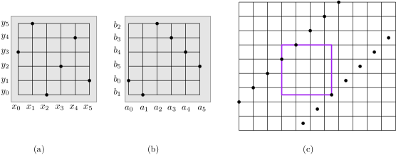
Figure 9: (a) A good square with six points. (b) Another good square with six points $p_{0},\ldots,p_{5}$ near integer grid points $(a_{i},b_{i})$, $i=0,1,2,3,4,5$, respectively. (c) An unpierced square of side-length $\approx 3.5$ in a lattice with $\lambda\approx\sqrt{2}$.

Claim 5.

Block $B$ contains at least one good square.

Proof.

Note that each row of $B$ has at most $100$ squares that are $x$-bad (otherwise a $1\times 6$ rectangle remains unpierced). Similarly, each column of $B$ has at most $100$ squares that are $y$-bad (otherwise a $6\times 1$ rectangle remains unpierced). Since each row or column of $B$ has $300$ squares, there are at most $300\cdot 100+300\cdot 100=60000$ bad squares in $B$. Taking into account that $B$ has $90000$ squares in total (and only a small number of squares are on its boundary), the claim immediately follows. ∎

Let now $S$ denote such a square. In the remainder of the proof we will only work with $S$ (and no other square). Let $p^{\prime}$ and $p^{\prime\prime}$ be the leftmost and respectively the lowest point in $\Lambda\cap S$ (it is possible that $p^{\prime}=p^{\prime\prime}$). Let $R$ denote the rectangle which is the intersection between the closed halfplane right of $p^{\prime}$, the closed halfplane above $p^{\prime\prime}$ and $S$. Note that both the width and the height of $R$ are strictly larger than $5$; $R$ contains exactly $6$ lattice points.

We finalize the proof by deducing certain properties for the relative position of the points in $\Lambda\cap S$ that in turn imply certain properties for the lattice $\Lambda$. Once a suitable restricted range is established, only two relevant cases remain, and for each we deduce that there are (many) unpierced $3\times 3$ squares. (Indeed, if there is an unpierced $w\times h$ rectangle amidst a point lattice, then there are infinitely many such rectangles.)

Pick a new orthogonal system $\Gamma$ whose origin is the left lower corner of $R$. Let $p_{0},p_{1},p_{2},p_{3},p_{4},p_{5}$ be the six points in $\Lambda\cap R$ ordered from left to right: $p_{i}=(x_{i},y_{i}),i=0,\ldots,5$. Observe that each of the $6$ points in $\Lambda\cap S$ lies in the neighborhood of a grid point in $\{0,1,2,3,4,5\}^{2}$. Let $(a_{i},b_{i})$ be the integer grid point near $p_{i}$; we have $a_{i}=i$, for $i=0,\ldots,5$. See Fig. 9 (b). Moreover, the corresponding grid points have no two $x$- or $y$-coordinates the same. As such, we have

$$x_{i} =i-\alpha_{i},\text{ for }i=0,1,2,3,4,5,\text{ where }\alpha_{i}\in[0,i/100],$$ (4)

$$y_{i} =b_{i}-\beta_{i},\text{ for }i=0,1,2,3,4,5,\text{ where }b_{i}\in\{0,1,2,3,4,5\},\beta_{i}\in[0,5/100],$$

$$b_{i} \neq b_{j}\text{ whenever }i\neq j,\text{ and }\min\{y_{i}\}=0.$$

By 1 we have $\lambda\leq 2\cdot 3^{1/4}<2.64$. Since $\lambda$ is close to a distance determined by points in $\mathbb{Z}^{2}$, this immediately implies that $\lambda\approx\sqrt{2}$ or $\lambda\approx\sqrt{5}$. More precisely, since each gap is between $1-0.01$ and $1$, the triangle inequality yields

$$\sqrt{2}-0.02\leq\lambda\leq\sqrt{2}\text{ or }\sqrt{5}-0.03\leq\lambda\leq\sqrt{5}.$$

We next rule out each of these two possibilities.

$\lambda$	Slope	$(b_{0},\ldots,b_{5})$	Comments
$\sqrt{2}$	$+1$	$(5,0,1,2,3,4)$	N/A
$\sqrt{2}$	$+1$	$(4,5,0,1,2,3)$	N/A
$\sqrt{2}$	$+1$	$(3,4,5,0,1,2)$	N/A
$\sqrt{2}$	$+1$	$(2,3,4,5,0,1)$	N/A
$\sqrt{2}$	$+1$	$(1,2,3,4,5,0)$	N/A
$\sqrt{2}$	$+1$	$(0,1,2,3,4,5)$	N/A
$\sqrt{2}$	$-1$	$(0,5,4,3,2,1)$	N/A
$\sqrt{2}$	$-1$	$(1,0,5,4,3,2)$	N/A
$\sqrt{2}$	$-1$	$(2,1,0,5,4,3)$	N/A
$\sqrt{2}$	$-1$	$(3,2,1,0,5,4)$	N/A
$\sqrt{2}$	$-1$	$(4,3,2,1,0,5)$	N/A
$\sqrt{2}$	$-1$	$(5,4,3,2,1,0)$	N/A

Table 1: Summary of cases for $\lambda\approx\sqrt{2}$.

Consider first the case $\lambda\approx\sqrt{5}$. This case corresponds to $\lambda$-lattice lines whose slopes are close approximations of $\{\pm 1/2,\pm 2\}$. We may assume (without loss of generality) that the slope of $\lambda$-lattice lines is $\approx 2$. Consider the line $\ell:y=2x+y_{0}$, where $y_{0}\in\{0,1,2,3,4,5\}$. Observe that the distance from $(3,y_{0})$ to $\ell$ is $6/\sqrt{5}$ (which is needed for $A\approx 6$). It follows that the only integer points in $\{0,1,2,3,4,5\}^{2}$ whose distance to $\ell$ is $6/\sqrt{5}$ correspond to or have the same $y$-coordinates as the integer points on $\ell$. In particular, we cannot have a lattice with $\lambda\approx\sqrt{5}$ because it would entail integer points $(a_{i},b_{i})$ with duplicate $x$- or $y$-coordinates.

Consider now the remaining case $\lambda\approx\sqrt{2}$. This would require consecutive parallel $\lambda$-lines of slope close to $1$ or $-1$ at distance $\approx 3\sqrt{2}$ (since $A\approx\sqrt{2}\cdot 3\sqrt{2}=6$ in this case). There are $12$ possible choices for $(b_{0},\ldots,b_{5})$; as listed in Table 1 (six for slope $+1$ and six for slope $-1$). Now it is easy to verify (refer to Fig. 9 (c)) that two parallel $\lambda$-lines with slope close to $1$ (or $-1$) at distance about $3\sqrt{2}$ leave unpierced certain axis-parallel squares of side-length about $3.5$, and thereby also the respective concentric smaller $3\times 3$ squares, which is a contradiction.

Consequently, $\pi_{L}(\mathcal{F}_{0})\geq 1/6+\varepsilon$, and the proof of Theorem 4 is complete. ∎

8 A sharper separation result

In this section we prove Theorem 5. Consider the $3$-rectangle family $\mathcal{F}_{0}=\{6\times 1,1\times 6,3\times 3\}$ from Section 7. The lower bound $\pi_{L}(\mathcal{F}_{0})\leq\frac{6}{31}$ is implied by the lattice with basis $u=[1,5/3]$, $v=[5/2,-1]$, shown in Fig. 7.

Let $\{u,v\}$ be a basis of an $\mathcal{F}_{0}$-piercing lattice $\Lambda$ satisfying properties P1–P3. Let $A$ denote the area of the fundamental parallelogram of $\Lambda$, and so its density is $1/A$. We will show that if $\Lambda$ has optimal density $\pi_{L}(\mathcal{F}_{0})$ then $A=\frac{31}{6}$, which immediately implies the claimed gap; indeed, $6/A=\frac{36}{31}$. In the remainder of the proof we focus on the upper bound $A\leq\frac{31}{6}$. By 1, we have $A\leq A_{\min}=6$. We may thus assume that $\frac{31}{6}\leq A\leq 6$.

Remark.

In order to get tighter estimates on the lattice parameters, one may be tempted to further assume that $\frac{31}{6}\leq A\leq\frac{31}{6}+\varepsilon$, for some small $\varepsilon>0$, as suitable. However, this would be incorrect. Recall that an optimal lattice is (i) piercing and (ii) tight. If there exists a piercing lattice with $A>\frac{31}{6}+\varepsilon$, its basis vectors can be shrunk so that the resulting lattice is still $\mathcal{F}_{0}$-piercing and its cell area $A$ belongs to the short interval indicated above. But shrinking its basis vectors will maintain (i) but not (ii). Because our first algorithm crucially relies on (ii) tightness, we need to respect the upper bound $A\leq 6$ (and cannot use the stronger version $A\leq 31/6+\varepsilon$).

$\mathcal{F}_{0}$-specific bounds.

Lemma 6.

Write $\lambda=|u|$. The following inequalities hold:

1. $1.217\leq\lambda\leq 2.633$

2. $1.962\leq\mu\leq 3\sqrt{2}$

3. $\frac{31}{6\lambda}\leq|v|\leq 4.994$

Proof.

(i) By Lemma 1 we have

$$\lambda\leq\sqrt{\frac{2A}{\sqrt{3}}}\leq\sqrt{\frac{12}{\sqrt{3}}}\leq 2.633,$$

proving the upper bound.

Observe that $\mu\leq 3\sqrt{2}$: indeed, any two parallel lines at distance at least $3\sqrt{2}$ leave a $3\times 3$ square unpierced. From $A=\lambda\mu$ we deduce that

$$\lambda=\frac{A}{\mu}\geq\frac{31/6}{3\sqrt{2}}\geq 1.217,$$

proving the lower bound.

(ii) We have $A=\lambda\mu$, hence

$$\mu=\frac{A}{\lambda}\geq\frac{31/6}{2.633}\geq 1.962,$$

proving the lower bound. The upper bound was proven in item (i) above.

(iii) From the chain of inequalities

$$\frac{31}{6}\leq A=\lambda\mu=|u||v|\sin\alpha\leq|u||v|,$$

one immediately obtains $|v|\geq\frac{31}{6\lambda}$, proving the lower bound. Finally, we have

$$|v|^{2}\leq\lambda^{2}+\mu^{2}\leq 6.9327+18=24.9327,$$

whence $|v|\leq 4.994$, proving the upper bound. ∎

Tight constraints for rectangles in $\mathcal{F}_{0}$.

Recall that $u=[a,b]$, $v=[c,-d]$ with $a,b,c,d\geq 0$, and $b>0$ is a vector basis of $\Lambda$, and that $x$-tight constraints are of the form

$$i_{s}\cdot a+j_{s}\cdot c=w_{s},$$

where $w_{s}$ is the width of a rectangle in $\mathcal{F}_{0}$. Next we consider the tight constraints for each rectangle in $\mathcal{F}_{0}=\{6\times 1,1\times 6,3\times 3\}$.

Lemma 7.

Assume that $i\cdot a+j\cdot c=6$, where $i,j\in\mathbb{Z}$, is an $x$-tight constraint for a $6\times 1$ rectangle $R$ supported on the left by the origin $o$. Then $i,j\in\mathbb{N}$ and $i+j\leq 8$.

Proof.

Suppose that the $x$-tight constraint is given by $o$ and $q=iu+jv$, where $p=iu$. Since $\max(|u|,|v|)=|v|\leq 4.994<6$ a shortest $uv$-path between $o$ and $q$ in $\Lambda$ has nonnegative coefficients, thus $i,j\in\mathbb{N}$. We may assume without loss of generality that $i,j\geq 1$. Let $\Delta{opq}$ be the triangle with one vertex at the origin and whose two other vertices are $p=iu$, and $q=iu+jv$. Refer to Fig. 10.

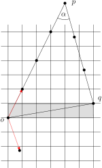
Figure 10: The triangle $\triangle{opq}$.

Let $\alpha,\beta,\gamma$ be the interior angles in $\Delta{opq}$. By the law of sines we have

$$\frac{|oq|}{\sin\alpha}=\frac{|pq|}{\sin\beta}=\frac{|op|}{\sin\gamma}.$$

In addition we have

$$|oq| \leq\sqrt{6^{2}+1^{2}}=\sqrt{37},\text{ since }R\text{ is supported by }o\text{ and }q\text{ from left and right, and}$$

$$\alpha \geq 45^{\circ}\text{ by Lemma~{}\ref{lem:angle}.}$$

It follows that

$$|op|+|pq| =\frac{\sin\beta+\sin\gamma}{\sin\alpha}\,|oq|\leq\frac{2\sin\frac{180^{\circ}-\alpha}{2}}{\sin\alpha}\,|oq|,$$ (5)

$$=\frac{2\cos\frac{\alpha}{2}}{2\sin\frac{\alpha}{2}{\cos\frac{\alpha}{2}}}\,|oq|=\frac{1}{\sin\frac{\alpha}{2}}\,|oq|$$

$$\leq\frac{1}{\sin 22.5^{\circ}}\,\sqrt{37}\leq 15.896.$$

First we note an easy bound

$$i+j\leq\left\lfloor\frac{|op|+|pq|}{\lambda}\right\rfloor\leq\left\lfloor\frac{15.896}{1.217}\right\rfloor=13.$$

Observe that if $i\geq 8$ then $j\geq 2$: indeed, since $\alpha\geq 45^{\circ}$, $|op|\geq 8\lambda>9.73$ implies $|pq|>4.994\geq|v|$. Similarly, if $j\geq 8$ then $i\geq 2$ by a symmetric argument. If $i\geq 8$ and $j\geq 2$ then (by routine algebraic verification) we have

$$|op|+|pq|\geq 8\lambda+2\,\frac{31}{6\lambda}>18.226>15.896,$$

in contradiction with (5). The case $j\geq 8$ and $i\geq 2$ can be dismissed by a symmetric argument. We can therefore subsequently assume that $1\leq i,j\leq 7$. Assume for contradiction that $i+j\geq 9$ where $2\leq i,j\leq 7$. Then

$$|op|+|pq|\geq i\lambda+(9-i)\,\frac{31}{6\lambda}\text{ for some }i\in\{2,3,4,5,6,7\}.$$

A routine algebraic verification shows that

$$ix+(9-i)\,\frac{31}{6x}>17>15.896,\text{ for }2\leq i\leq 7\text{ and }1.217\leq x\leq 2.633.$$

This is in contradiction with (5) and the claimed bound $i+j\leq 8$ follows. ∎

Lemma 8.

Assume that $i\cdot b+j\cdot d=1$, where $i,j\in\mathbb{Z}$, is a $y$-tight constraint for a $6\times 1$ rectangle $R$ supported on the left by the origin $o$. Then $|i|+|j|\leq 8$.

Proof.

Assume that the $y$-tight constraint is given by $p$ and $q$, where $p-q=iu+jv$. If $i=0$ or $j=0$ the inequality is obvious. In the remaining case, consider the triangle made by the lattice path connecting $p$ and $q$ (according to $p-q=iu+jv$) and proceed as in the proof of Lemma 7. ∎

Lemma 9.

Assume that $i\cdot a+j\cdot c=3$, where $i,j\in\mathbb{Z}$, is an $x$-tight constraint for a $3\times 3$ rectangle $R$ supported on the left by the origin $o$. Then $i,j\in\mathbb{N}$ and $i+j\leq 6$.

Proof.

Suppose that the $x$-tight constraint is given by $o$ and $q=iu+jv$, where $p=iu$. Observe that a shortest $uv$-path between $o$ and $q$ in $\Lambda$ has nonnegative coefficients, thus $i,j\in\mathbb{N}$. Note that the diagonal of the $3\times 3$ square is $3\sqrt{2}$ and then proceed as in the proof of Lemma 7.

We may assume without loss of generality that $i,j\geq 1$. Let $\Delta{opq}$ be the triangle with one vertex at the origin and whose two other vertices are $p=iu$, and $q=iu+jv$. Let $\alpha,\beta,\gamma$ be the interior angles in $\Delta{opq}$. By the law of sines we have

$$\frac{|oq|}{\sin\alpha}=\frac{|pq|}{\sin\beta}=\frac{|op|}{\sin\gamma}.$$

In addition we have

$$|oq| \leq 3\sqrt{2},\text{ since }R\text{ is supported by }o\text{ and }q\text{ from left and right, and}$$

$$\alpha \geq 45^{\circ}\text{ by Lemma~{}\ref{lem:angle}.}$$

It follows that

$$|op|+|pq|\leq\frac{1}{\sin\frac{\alpha}{2}}\,|oq|\leq\frac{1}{\sin 22.5^{\circ}}\,3\sqrt{2}\leq 11.089,$$ (6)

which further yields

$$i+j\leq\left\lfloor\frac{|op|+|pq|}{\lambda}\right\rfloor\leq\left\lfloor\frac{11.089}{1.217}\right\rfloor=9.$$

Assume for contradiction that $i+j\geq 7$. Then

$$|op|+|pq|\geq i\lambda+(7-i)\,\frac{31}{6\lambda},\text{ where }1\leq i\leq 6.$$

A routine algebraic verification shows that

$$ix+(7-i)\,\frac{31}{6x}>11.547>11.089,\text{ for }1\leq i\leq 6\text{ and }1.217\leq x\leq 2.633.$$

This is in contradiction with (6) and the claimed bound follows. ∎

Lemma 10.

Assume that $i\cdot b+j\cdot d=3$, where $i,j\in\mathbb{Z}$, is a $y$-tight constraint for a $3\times 3$ rectangle $R$ supported on the left by the origin $o$. Then $|i|+|j|\leq 6$.

Proof.

Observe that the diagonal of the $3\times 3$ square is $3\sqrt{2}$. Then proceed as in the proof of Lemma 9. ∎

The proofs of the next two lemmas are analogous to the proof of Lemma 7, as they lead to the same calculation.

Lemma 11.

Assume that $i\cdot a+j\cdot c=1$, where $i,j\in\mathbb{Z}$, is an $x$-tight constraint for a $1\times 6$ rectangle $R$ supported on the left by the origin $o$. Then $|i|+|j|\leq 8$.

Lemma 12.

Assume that $i\cdot b+j\cdot d=6$, where $i,j\in\mathbb{Z}$, is a $y$-tight constraint for a $1\times 6$ rectangle $R$ supported on the left by the origin $o$. Then $i,j\in\mathbb{N}$ and $i+j\leq 8$.

Proof.

Suppose that the $y$-tight constraint is given by $p$ and $q$, where $p$ and $q$ are on the lower and the upper side of $R$, respectively. Let $\rho=iu+jv$ be a shortest $uv$-path between $p$ and $q$ in $\Lambda$. Observe that the coefficient of $u$ in $\rho$ must be positive and the coefficient of $v$ must be negative. Recall that $v=[c,d)$ where $d<0$, whence $i,j\in\mathbb{N}$. Note that the diagonal of the $1\times 6$ square is $\sqrt{37}$ and then proceed as in the proof of Lemma 7. ∎

Lemma 13.

If $u=[a,b]$, $v=[c,-d]$ with $a,b,c,d\geq 0$, and $b>0$, and $\Lambda$ has optimal $\mathcal{F}_{0}$-piercing density $1/A$, then $A\leq\frac{31}{6}$.

Proof.

Note that $A=ad+bc$ and since $\Lambda$ has minimum $\mathcal{F}_{0}$-piercing density, $A$ is maximized. In particular, we have $A\geq\frac{31}{6}$. We may assume that the properties P1–P3 hold.

For the special case of the $3$-family rectangle $\mathcal{F}_{0}=\{6\times 1,1\times 6,3\times 3\}$ we have $k=6$; recall that $k$ is the maximum rectangle dimension (width or height). The computer program implementation follows the outline in Section 5. It performs the following steps:

1. Generate all $x$-equations for the three rectangles in $\mathcal{F}_{0}$.

2. Generate all $y$-equations for the three rectangles in $\mathcal{F}_{0}$.

3. Generate system solutions for $2\times 2$ systems in $a,c$ (from $x$-equations) according to the specifications in Lemmas 7, 9 and 11.

4. Generate system solutions for $2\times 2$ systems in $b,d$ (from $y$-equations) according to the specifications in Lemmas 8, 10 and 12.

5. Generate candidate lattices from system solutions in $a,c$ and $b,d$.

6. For each candidate lattice test if its density is in required interval $[5.16,6]$ and if the lattice is $\mathcal{F}_{0}$-piercing: Generate the lattice points in a $6\times 6$ board; compute the funnel (the funnel has generally fewer than ten points); use a brute force approach to examine the maximal empty rectangles supported from the left by the origin; the existence of horizontal lattice lines yields an easy special case of maximal empty rectangles supported from below.

7. Output valid lattices, i.e., those passing the piercing test, by increasing density (i.e., by decreasing area $A$).

The program finds the optimal piercing density is $6/31$ (i.e., $1/A$ where $A=31/6$); there are no $\mathcal{F}_{0}$-piercing lattices found with $A>31/6$. ∎

The output produced by an actual program execution when it is run with $A\in[5.16,6.00]$ appears in Section A of the appendix. In general, the same lattice may be generated from different pairs of linear systems. After removing obvious duplicates one ends up with the two lattices specified in first two rows of Table 2. These lattices are the only optimal $\mathcal{F}_{0}$-piercing lattices with density $6/31$.

$a$	$b$	$c$	$d$	Area ($A$)
$1/1$	$5/3$	$5/2$	$1/1$	$31/6=5.166\ldots$
$5/3$	$1/1$	$8/3$	$3/2$	$31/6=5.166\ldots$
$1/1$	$1/1$	$1/1$	$4/1$	$5/1=5.00$
$1/1$	$2/1$	$1/1$	$3/1$	$5/1=5.00$

Table 2: First two rows: optimal $\mathcal{F}_{0}$-piercing lattices with density $6/31$ (the first two entries from the output in Section A). Last two rows: optimal $\mathcal{F}_{1}$-piercing lattices with density $1/5$ (the first two entries from the output in Section B).

9 An even sharper separation

Theorem 4 shows a preliminary separation result. In this section we prove Theorem 6. Consider the (extended) family $\mathcal{F}_{1}=\{6\times 1,1\times 6,3\times 3,4\times 2,2\times 4\}$; note that $\mathcal{F}_{1}\supset\mathcal{F}_{0}$. It is easily verified by inspection that the periodic piercing set in Fig. 1 is also a valid piercing set for $\mathcal{F}_{1}$; it is repeated here for convenience in Fig. 11.

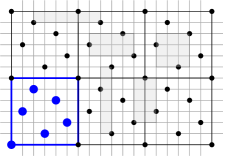
Figure 11: This non-lattice periodic grid point-set pierces all translates of $\mathcal{F}_{1}=\{6\times 1,1\times 6,3\times 3,4\times 2,2\times 4\}$.

A similar verification by inspection shows that none of the two optimal $\mathcal{F}_{0}$-piercing lattices in Fig. 12 pierces both rectangles in $\mathcal{F}_{1}\setminus F_{0}$; indeed, the first lattice does not pierce the $2\times 4$ rectangle, and the second lattice does not pierce the $4\times 2$ rectangle. Since these are the only two optimal $\mathcal{F}_{0}$-piercing lattices, we conclude that the separation gap implied by $\mathcal{F}_{1}$ is even larger.

Next we provide the technical details that provide specifications for adapting the program for computing the optimal lattice piercing density for $\mathcal{F}_{1}$. Since $\mathcal{F}_{0}\subset\mathcal{F}_{1}$ the bounds in Lemmas 6 through 12 still hold. In addition, the following specific lemmas for the new rectangles allow for an efficient implementation of the program. Since they are analogous to Lemmas 7 through 12, their proofs are omitted. It should be noted that the slightly weaker versions of these lemmas with $6$ replaced by $8$ suffice for the program implementation (at a modest increase in complexity) and the corresponding proofs are even simpler.

Lemma 14.

Assume that $i\cdot a+j\cdot c=4$, where $i,j\in\mathbb{Z}$, is an $x$-tight constraint for a $4\times 2$ rectangle $R$ supported on the left by the origin $o$. Then $|i|+|j|\leq 6$.

Lemma 15.

Assume that $i\cdot b+j\cdot d=2$, where $i,j\in\mathbb{Z}$, is a $y$-tight constraint for a $4\times 2$ rectangle $R$ supported on the left by the origin $o$. Then $|i|+|j|\leq 6$.

Lemma 16.

Assume that $i\cdot a+j\cdot c=2$, where $i,j\in\mathbb{Z}$, is an $x$-tight constraint for a $2\times 4$ rectangle $R$ supported on the left by the origin $o$. Then $|i|+|j|\leq 6$.

Lemma 17.

Assume that $i\cdot b+j\cdot d=4$, where $i,j\in\mathbb{Z}$, is a $y$-tight constraint for a $2\times 4$ rectangle $R$ supported on the left by the origin $o$. Then $|i|+|j|\leq 6$.

The maximum rectangle dimension for the family $\mathcal{F}_{1}=\{6\times 1,1\times 6,3\times 3,4\times 2,2\times 4\}$ is still $k=6$. The program finds the optimal piercing density is $1/5$ (i.e., $1/A$ where $A=5$); there are no $\mathcal{F}_{1}$-piercing lattices found with $A>5$.

The output produced by an actual program execution when it is run with $A\in[5.00,5.16]$ appears in Section B of the appendix. Again, note that the same lattice can be generated from different pairs of linear systems. After removing obvious duplicates one ends up with the two lattices specified in the last two rows of Table 2. These lattices are the only optimal $\mathcal{F}_{1}$-piercing lattices with density $1/5$.

10 Conclusion

We list several directions to be explored.

1. Given a family $\mathcal{F}$ of $n$ axis-parallel rectangles, what is the computational complexity of determining the translative piercing density $\pi_{T}(\mathcal{F})$ and the lattice piercing density $\pi_{L}(\mathcal{F})$ of $\mathcal{F}$? Is there a polynomial-time algorithm independent of $k$ for any of these problems?

2. What is the largest possible relative gap between the optimal lattice and non-lattice piercing densities for a family of axis-parallel rectangles? We have shown a lower bound of $1.2$ and an upper bound of $1.895$ (in a previous work) on this gap.

3. Is it true that $\pi_{T}(\mathcal{F})=\pi_{L}(\mathcal{F})$ for families $\mathcal{F}$ of two rectangles?

4. How does the gap between the optimal lattice and non-lattice piercing densities for families of axis-parallel boxes grow with the dimension of the space?

5. The two algorithms for finding an optimal piercing lattice appear to be extendable to piercing axis-parallel boxes in higher dimensions. This is left as an open problem.

Appendix A Program output

The program produces the following output when it is run with $A\in[5.16,6.00]$. The corresponding distinct lattices are shown in Fig. 12.

Output summary

Generating all equations

Number of equations is 230

Generate system solutions for 2x2 in x : a&c

Number of ac-solutions is 1663

Generate system solutions for 2x2 in y : b&d

Number of bd-solutions is 2007

Generate lattices from system solutions: a&c and b&d

Number of candidate lattices is 29642

Number of valid lattices with area in [5.160 , 6.000] =   4

Amax = 5.1667

Valid lattices with area in [5.160 , 6.000]:

a =  1/ 1  b =  5/ 3  c =  5/ 2  d =  1/ 1  Area= 31/ 6 =5.1667

System in a,c: 1*a + 2*c =  6, 1*a + 0*c =  1

System in b,d: 0*b + 1*d =  1, 3*b + -4*d =  1

a =  5/ 3  b =  1/ 1  c =  8/ 3  d =  3/ 2  Area= 31/ 6 =5.1667

System in a,c: 2*a + 1*c =  6, -1*a + 1*c =  1

System in b,d: 1*b + 0*d =  1, 3*b + 2*d =  6

a =  5/ 3  b =  1/ 1  c =  1/ 1  d =  5/ 2  Area= 31/ 6 =5.1667

System in a,c: 3*a + 1*c =  6, 0*a + 1*c =  1

System in b,d: 1*b + 0*d =  1, 1*b + 2*d =  6

a =  1/ 1  b =  5/ 3  c =  3/ 2  d =  8/ 3  Area= 31/ 6 =5.1667

System in a,c: 3*a + 2*c =  6, 1*a + 0*c =  1

System in b,d: -1*b + 1*d =  1, 2*b + 1*d =  6

Normal termination

Figure 12: The two optimal $\mathcal{F}_{0}$-piercing lattices of density $6/31$: Left: $u=[1,5/3]$, $v=[5/2,-1]$. Right: $u=[5/3,1]$, $v=[8/3,-3/2]$. The 2nd lattice is a reflection of the 1st one about the line $y=x$. Since $\mathcal{F}_{0}$ is preserved under this reflection, the two lattices are in some sense equivalent.

Appendix B Program output

The program produces the following output when it is run with $A\in[5.00,5.16]$. The corresponding distinct lattices are shown in Fig. 13.

Output summary

Generating all equations

Number of equations is 378

Generate system solutions for 2x2 in x : a&c

Number of ac-solutions is 3170

Generate system solutions for 2x2 in y : b&d

Number of bd-solutions is 3604

Generate lattices from system solutions: a&c and b&d

Number of candidate lattices is 19515

Number of valid lattices with area in [5.000 , 5.160] =   4

Amax = 5.0000

Valid lattices with area in [5.000 , 5.160]:

a =  1/ 1  b =  1/ 1  c =  1/ 1  d =  4/ 1  Area=  5/ 1 =5.0000

System in a,c: 1*a + 5*c =  6, 5*a + 1*c =  6

System in b,d: 1*b + 0*d =  1, -3*b + 1*d =  1

a =  1/ 1  b =  2/ 1  c =  1/ 1  d =  3/ 1  Area=  5/ 1 =5.0000

System in a,c: 1*a + 5*c =  6, 5*a + 1*c =  6

System in b,d: -1*b + 1*d =  1, 2*b + -1*d =  1

a =  1/ 1  b =  1/ 1  c =  4/ 1  d =  1/ 1  Area=  5/ 1 =5.0000

System in a,c: 2*a + 1*c =  6, 1*a + 0*c =  1

System in b,d: 0*b + 1*d =  1, 1*b + 0*d =  1

a =  2/ 1  b =  1/ 1  c =  3/ 1  d =  1/ 1  Area=  5/ 1 =5.0000

System in a,c: 0*a + 1*c =  3, -1*a + 1*c =  1

System in b,d: 0*b + 1*d =  1, 1*b + 0*d =  1

Normal termination

Figure 13: The two optimal $\mathcal{F}_{1}$-piercing lattices of density $1/5$: Left: $u=[1,1]$, $v=[1,-4]$. Right: $u=[1,2]$, $v=[1,-3]$.

References

- [1] P. Braß, W. Moser, and J. Pach, Research Problems in Discrete Geometry, Springer, New York, 2005.
- [2] T.M. Chan, Faster algorithms for largest empty rectangles and boxes, Proc. 37th International Symposium on Computational Geometry (SoCG 2021), LIPIcs series, vol. 189, Schloss Dagstuhl - Leibniz-Zentrum für Informatik, Germany, 2021, pp. 24:1–24:15. Preprint available at arXiv:2103.08043.
- [3] J. R. Correa, L. Feuilloley, P. Pérez-Lantero, and J. A. Soto, Independent and hitting sets of rectangles intersecting a diagonal line: algorithms and complexity, Discrete & Computational Geometry 53(2) (2015), 344–365.
- [4] A. Dumitrescu and J. Tkadlec, Piercing all translates of a set of axis-parallel rectangles, Proceedings of the 32nd International Workshop on Combinatorial Algorithms (IWOCA 2021), vol 12757 of LNCS, Springer, 2021, pp. 295–309. Preprint available at arXiv:2106.07459.
- [5] P. Erdős and J. Surányi, Topics in the Theory of Numbers, second edition, Springer, New York, 2003.
- [6] B. Grünbaum and G. C. Shephard, Tilings and patterns, Freeman and Company, New York, 1987.
- [7] A. Namaad, D.T. Lee, and W.-L. Hsu, On the maximum empty rectangle problem, Discrete Applied Mathematics, 8 (1984), 267–277.
- [8] J. Pach and P. K. Agarwal, Combinatorial Geometry, John Wiley, New York, 1995.
- [9] C. Papadimitriou, Computational Complexity, Addison-Wesley, Reading, MA, 1994.
- [10] C. Papadimitriou, On the complexity of integer programming, Journal of ACM, 28(4) (1981), 765–768.
- [11] D. F. Riddle, Calculus and Analytic Geometry, Wadsworth Publishing Co., Belmont, CA, 1970.
- [12] V. Vazirani, Approximation Algorithms, Springer Verlag, New York, 2001.