Autonomous Vehicle Parking in Dynamic Environments: An Integrated System with Prediction and Motion Planning

Abstract

This paper presents an integrated motion planning system for autonomous vehicle (AV) parking in the presence of other moving vehicles. The proposed system includes 1) a hybrid environment predictor that predicts the motions of the surrounding vehicles and 2) a strategic motion planner that reacts to the predictions. The hybrid environment predictor performs short-term predictions via an extended Kalman filter and an adaptive observer. It also combines short-term predictions with a driver behavior cost-map to make long-term predictions. The strategic motion planner comprises 1) a model predictive control-based safety controller for trajectory tracking; 2) a search-based retreating planner for finding an evasion path in an emergency; 3) an optimization-based repairing planner for planning a new path when the original path is invalidated. Simulation validation demonstrates the effectiveness of the proposed method in terms of initial planning, motion prediction, safe tracking, retreating in an emergency, and trajectory repairing.

I Introduction

Fully autonomous parking [1, 2] remains challenging especially in a dynamic environment with multiple independent agents, not only because it involves motion planning in a tight space, but also because autonomous vehicles (AVs) should intelligently react to the surrounding vehicles, i.e., obstacle vehicles (OVs). In contrast to driving on roads or highways, vehicle motions in parking areas do not have a clear set of rules to follow and largely depend on the driver’s intention or even skill level. These make the environment prediction in parking challenging, hence an autonomous parking system that integrates both prediction and planning is possibly necessary.

Motion prediction is crucial because it determines the safety constraints of the planning modules and thus the feasibility and smoothness of the motion plan [3]. Particularly, an accurate short-term motion prediction enables the AV to plan and react safely to the OVs; whereas long-term plan/mode prediction allows the AV to plan more efficiently and smoothly. This work proposes a model-based hybrid predictor to perform both short-term motion and long-term mode predictions by observing the poses of OVs. A major challenge in short-term prediction is to estimate the OV’s steering angle. We use extended Kalman filter (EKF) to reconstruct OV’s velocity, and then, resort to an adaptive observer for the steering estimation. Despite of the difficulty in predicting exact long-term motions, we observe that a driver generally follows some routes as a result of driving conventions (e.g., cars should stay on their left hand side in Japan). Also, vehicles’ motion throughout parking/leaving can be captured by several “modes” (e.g., maneuvering into/out of tight-spaces and cruising on aisles). Based on these two priors, we use a cost-map [4, 5] to capture these routes, combine the short-term predictions to determine OVs’ modes, and make long-term predictions.

Motion planning for AVs is another challenge in parking scenarios. General motion planning algorithms [6, 7, 8, 9, 10, 11] are not directly suitable for parking in the presence of OVs which requires rapid replanning for complicated driving maneuvers. On the other hand, motion planners specialized in autonomous parking either fail to integrate short-horizon planning with long-horizon planning or cannot incorporate online path repairing upon new obstacles in dynamic environments [12, 13, 14, 2, 15, 16]. A scenario-aware planner that implements multiple strategies can be effective in terms of computation time, leading to a high replanning rate, and possibly safety guarantees. In this work, we first generate a long-term motion reference with Bi-Directional A-Search Guided Tree (BIAGT) [17]. Then, a strategic motion planner, based on the results of the hybrid environment predictor, implements three strategies: 1) model predictive control (MPC)-based safety controller [18] for trajectory tracking if the reference remains valid regarding the environment, 2) search-based retreat-planning that quickly finds an evasion path in an emergency, and 3) optimization-based repair-planning when the reference is invalidated.

This work presents an integrated system for autonomous vehicle parking in dynamic environments. Main contributions are threefold as follows:

• A model-based hybrid environment predictor predicts short-term motions and long-term modes.

• A strategic motion planner is presented to efficiently plan under different situations.

• Simulation is performed to show the effectiveness of the proposed system.

II Related Works

II-A Predictor

Research in vehicle motion prediction has attracted a lot of interests, and results in numerous contributions, e.g., short-term motion prediction methods [19, 20, 21] and long-term plans/modes prediction methods [20, 21, 22, 23, 24, 25, 26]. It is arguably true that most research in this area is related to road driving. Interested readers are referred to an extensive survey in [27]. In contrast, vehicle motion prediction in parking is less explored. In [28], an interacting multiple model (IMM) filter is used to predict short-term trajectories in parking. Focusing on long-term prediction, [29] first trains a trajectory cluster classifier, and then acquires the mean-value trajectory of the classified cluster. In [24], the classified driver’s intent and the vehicle’s pose history are used to generate short-term motion predictions with a Long Short-Term Memory network. Purely data driven methods are not desirable for two reasons: 1) the lack of guarantees; 2) their performance depends largely on the training data set, and they may present a larger prediction error if the data set is chosen poorly. Prediction network over fitting may also be a concern. To the best of our knowledge, there are not extensive studies on a predictor fusing both short-term and long-term predictions for parking.

II-B Planning

Prevailing motion planning approaches fall into three categories: search-based [30, 31, 32], sampling-based [33, 34, 35] and optimization-based [36, 37, 38, 39]. Sampling-based planners could raise concerns in risk-sensitive tasks due to their non-deterministic nature, while optimization-based planners are only locally optimal and often need to work with global planners [40, 41, 42, 39, 43]. Various search-based motion planners are widely adopted by autonomous vehicles for their computation efficiency with well-chosen motion primitives and heuristics [44, 6, 45, 46, 47, 48, 49, 50].

If the parking environment changes, the initial long-term trajectory may need to be repaired. Real-time trajectory repairing methods include online heuristic update [51, 52, 53], pruning and reconnecting sampling-based search structures [54, 55, 56, 57], and spline-based kinodynamic search [58, 59]. The heuristic update method is not directly applicable to our tree-based search structure in BIAGT and pruning is less efficient for parking scenarios. Spline-based kinodynamic search is relatively efficient but the original trajectory is not utilized. On the other hand, we observe that alternative feasible solutions in the repairing scenarios are often in the same homotopy class as the original trajectory. Therefore, optimization-based methods [60, 37, 58] become suitable candidates for repairing an existing path.

II-C Parking system

As for system-level strategies for AV parking, [61] and [62] present autonomous parking systems to park in static environments. In [28], IMM is used for prediction with a sampling-based method for planning. The method in [22] first predicts the strategy of OVs, and then selects the navigation strategy of the ego AV. However, the AV only traverses the roads of the parking lot but do not perform parking maneuvers. Instead, our work aims at the more complete approach of an integrated parking system that makes both short-term and long-term predictions of the environment and utilize them in the strategic planning for parking.

III Methods

III-A Problem Statement

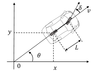
Figure 1: The simplified bicycle vehicle model. $L$ is the distance between the axis of the rear wheels and the axis of the front wheels.

Consider the planning problem with vehicle dynamics:

$$\small\dot{X}=f(X)+g(X,u),$$ (1)

where $X=[x,y,\theta]^{\top}$ denotes the 2D coordinates and the vehicle heading, and $u=[\delta,v]^{\top}$ is the control input that includes longitudinal velocity and steering angle. A collision-free configuration space $\mathcal{C}_{free}\subset{\mathbb{R}}^{n_{c}}$ is the set of configurations at which the vehicle has no intersection with the obstacles. The motion planning problem considered in this paper is defined as follows:

Problem III.1

Given an initial configuration $X_{0}\in\mathcal{C}_{free}$, a goal configuration $X_{f}\in\mathcal{C}_{free}$, and system (1), find a feasible trajectory $\mathcal{P}_{t}$ which

1. starts at $X_{0}$ and ends at $X_{f}$, while satisfying (1); and

2. lies in the collision-free configuration space $\mathcal{C}_{free}$.

We use the bicycle model, illustrated by Fig. 1, to represent the vehicle motion. The discrete-time model is obtained through Euler discretization as follows:

$$\begin{bmatrix}x_{k+1}\\ y_{k+1}\\ \theta_{k+1}\end{bmatrix}=\begin{bmatrix}x_{k}\\ y_{k}\\ \theta_{k}\end{bmatrix}+\begin{bmatrix}v_{k}T_{s}\cos(\theta_{k})\\ v_{k}T_{s}\sin(\theta_{k})\\ v_{k}T_{s}\frac{\tan{\delta_{k}}}{L}\end{bmatrix},$$ (2)

where $T_{s}$ is the sampling time.

III-B Proposed Architecture

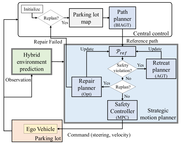
Figure 2: The integrated prediction and planning system.

Fig. 2 shows the architecture of the proposed system. The two main components are the hybrid environment predictor (Section III-C) and the strategic motion planner (Section III-D). During run-time, the central control first processes the parking lot map $M_{map}$ and generates an initial long-term trajectory $\mathcal{P}_{ref}$. We use BIAGT since it is guaranteed to plan a trajectory that brings the ego AV exactly to the goal, an important feature for parking in a tight space. The hybrid environment predictor monitors the environment and predicts the movements of the OVs. Based on the prediction, the strategic motion planner first checks if the ego AV is violating the safety margin. If not, it checks if $\mathcal{P}_{ref}$ needs to be repaired due to the OV. If any of these situations occurs, $\mathcal{P}_{ref}$ will be updated. Finally, an MPC-based safety controller plans a collision free motion that tracks the latest $\mathcal{P}_{ref}$ in the dynamic environment. If the repair-planner cannot succeed, it requests the central control to update the map and regenerate a reference trajectory.

III-C Hybrid Environment Predictor

The hybrid environment predictor (summarized in Alg. 1) contains three main parts: motion estimation, motion prediction, and mode estimation of OVs.

III-C1 Cascaded motion estimation

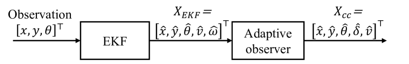
Figure 3: The architecture of the cascade motion estimator.

Motion estimation has been studied in, e.g. [24, 28], where the state $X$ is reconstructed from the measurement of $(x,y)$ based on the unicycle model. Such a treatment is not sufficient for vehicle parking, where frequent changes of moving direction and steering actions are involved. To accurately predict the short-term motion of the OV, it is advantageous to reconstruct the control input $u$. One can either pose it as an unknown input estimation problem [63] or augment the OV’s system state with the control input and solve a state estimation problem. Assume that the OV motion evolves according to the model (2). We obtain the augmented model of the OV by assuming that control input $(\delta,v)$ are piecewise constant, and estimate the augment state $[x,y,\theta,\delta,v]^{\top}$.

Given the nonlinear augmented model, it is natural to apply well-established nonlinear state estimators such as EKF or particle filter for state estimation. We observe that it is not straightforward to tune EKF for accurate estimation of the steering angle. This is partially attributed to the term $v\tan(\delta)$ which involves the multiplication of unmeasured states. Meanwhile, the heavy computation presents a hurdle for the adoption of particle filter.

A cascaded motion estimator (Fig. 3) is proposed to estimate the OV motion. The velocity estimation resorts to EKF and is based on the following discrete-time model:

$$\begin{bmatrix}x_{k+1}\\ y_{k+1}\\ \theta_{k+1}\\ v_{k+1}\\ \omega_{k+1}\end{bmatrix} =\begin{bmatrix}x_{k}+v_{k}T_{s}\cos(\theta_{k})\\ y_{k}+v_{k}T_{s}\sin(\theta_{k})\\ \theta_{k}+T_{s}\omega_{k}\\ v_{k}\\ \omega_{k}\end{bmatrix}+q_{k},\;q_{k}\sim\mathcal{N}(0,Q),$$ (3)

$$z_{k} =X_{OV,k}+r_{k},$$

where $\omega$ is the yaw rate, $q$ is the disturbance, $z_{k}=[z_{x,k},z_{y,k},z_{\theta,k}]^{\top}$ is the measurement, $X_{OV,k}=[x_{k},y_{k},\theta_{k}]^{\top}$, and $r_{k}\sim\mathcal{N}(0,R)$. The EKF outputs $X_{EKF,k}=[\hat{x}_{k},\hat{y}_{k},\hat{\theta}_{k},\hat{v}_{k},\hat{\omega}_{k}]^{\top}$. The estimation of the steering action is based on the following model

$$\omega=vs,\quad z_{\theta}=\theta,$$ (4)

where $z_{\theta}$ is the measurement and $s=\frac{\tan{\delta}}{L}$. We construct an adaptive observer as follows:

$$M_{k+1} =M_{k}-T_{s}(gM_{k}+\hat{v}_{k}),$$ (5)

$$\hat{s}_{k+1} =\hat{s}_{k}+T_{s}(\lambda M_{k}(z_{\theta}-\hat{\theta}_{a,k})),$$

$$\hat{\theta}_{a,k+1} =\hat{\theta}_{a,k}+T_{s}(\hat{s}_{k}\hat{v}_{k}+g(z_{\theta}-\hat{\theta}_{a,k})+M_{k}(\lambda M_{k}(z_{\theta}-\hat{\theta}_{a,k})),$$

where $M$ is an auxiliary signal, $g,\lambda\in\mathcal{R}$ are observer gains, $\hat{\theta}_{a}$ is the estimated heading angle, and $\hat{v}$ is the velocity estimated by EKF. The estimated steering angle can be calculated with $\hat{s}$, i.e., $\hat{\delta}=\tan^{-1}(\hat{s}L)$. It is not hard to verify that as long as $\hat{v}\rightarrow v$ and $v$ is non-zero, the steering angle estimate is guaranteed to converge to its true value as $t\rightarrow\infty$. The output of the cascade motion estimator is denoted as $X_{cc,k}=[\hat{x}_{k},\hat{y}_{k},\hat{\theta}_{k},\hat{\delta}_{k},\hat{v}_{k}]^{\top}$.

III-C2 Short-term motion prediction

For the sake of computation efficiency, we assume the short-term motion of an OV is fully captured by the mean value of the state $X_{cc}$, and its covariance. For the mean value, we propagate the estimated states $X_{cc,k}$ forward and obtain a short-term prediction $\mathbf{X}_{H,k}=[X_{1,k}^{\top},\dots,X_{H,k}^{\top}]^{\top}$ for the future $H$ steps of the time horizon. Similarly, forward propagation is carried out to obtain the covariance matrices $Pm_{H,k}=\{Pm_{k+1},\dots,Pm_{k+H}\}$ according to EKF’s forward prediction formula. These information will facilitate long-term prediction and be used to determine the safety margin for each future time step.

III-C3 Long-term mode prediction

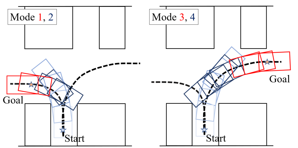
Figure 4: There are 2 routes (black dashed lines) and 2 main modes (red for “cruising” and blue for “maneuvering”) in this example, resulting in a total of 4 modes for the OV: 1) cruise(exit) left; 2) maneuver left; 3) cruise(exit) right; 4) maneuver right.

OV’s long-term motion is dependent on the history of its state, the dynamic model, and its relative movement against the environment, where the first two factors are captured to some extent by the short-term motion prediction. In order to exploit the relative movement against the environment, [4] and [5] introduced a cost map to capture an OV’s possible long-term movements. We adopt the same idea and construct a cost map, $M_{route}$ using a route planner [64], where the cost map contains possible routes that the OV will take (6). Also, we recognize that a vehicle in the parking lot normally runs in two modes, “maneuvering” and “cruising”. Vehicles in maneuvering mode change the steering frequently and deviate from the routes (black dashed line in Fig. 4) in the cost map in order to park or leave the narrow parking spot. Vehicles in cruising mode have small or steady steering angles and generally follow one of the routes. Vehicles are in this mode when they first enter the parking lot and are approaching a parking spot or when they got out of the parking spot and are leaving the parking lot. Including the route information, an OV that has $n$ routes to follow will have $2n$ possible modes (Fig. 4). To determine the mode $m$ at time step $k$, i.e., $m_{k}$, Bayesian framework is employed to keep track of the belief of each mode, i.e., $b(m_{k})$. The process is described in Alg. 1, lines 5$\sim$8. We perform the prior believe update $p(m_{k})=T_{b}b(m_{k-1})$ based on the previous belief, $b(m_{k-1})$. The posterior $p(m_{k}|X_{cc,k},\mathbf{X}_{H,k})$ is proportional to the prior multiplied with the conditional probability of the motion estimation and prediction given the mode, i.e., $p(m_{k})p(X_{cc,k},\mathbf{X}_{H,k}|m_{k})$. The Boltzmann policy is one common way to design this conditional probability [65], i.e., $p(X_{cc,k},\mathbf{X}_{H,k}|m_{k})\propto\exp(-M_{route}(m_{k},X_{cc,k},\mathbf{X}_{H,k}))f(m_{k},X_{cc,k})$. The function $M_{route}(m_{k},X_{cc,k},\mathbf{X}_{H,k})$ compares the OV states and predictions with the routes:

$$M_{route}(m_{k},X_{cc,k},\mathbf{X}_{H,k})= \min_{i}\|X_{m_{k},i}-X_{cc,k}\|^{2}_{W_{1}}$$ (6)

$$+\sum_{h}\min_{i}\|X_{m_{k},i}-X_{h,k}\|^{2}_{W_{2}},$$

where $X_{m_{k},i}$ is the $ith$ waypoint of the route in mode $m_{k}=m$, $m\in\{1,\dots,2n\}$, $\|\mathrm{v}\|^{2}_{W}=\mathrm{v}^{\top}W\mathrm{v}$, and $W_{1}$ and $W_{2}$ are weighting matrices. The function $f(m_{k},X_{cc,k})$ is proportional to the magnitude of the OV’s steering angle and the deviation of the OV’s heading angle from the final heading angle of the route. Finally, we normalize $p(m_{k}|X_{cc,k},\mathbf{X}_{H,k})$ to obtain $b(m_{k})$ and take the value of $m_{k}$ with the largest belief to be $\hat{m}_{k}$.

III-C4 Safety margin and safety bound

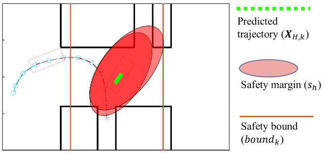
Figure 5: The hybrid predictor predicts a short-term OV trajectory (green line) and use it with mode prediction to generate the safety margins for $h=1$ and $h=H$ and the safety bound.

When the OV is in cruising mode, the predictor calculates the safety margins $\mathbf{s}_{H,k}=[s_{k+1}^{\top},\dots,s_{k+H}^{\top}]^{\top}$ (red areas in Fig. 5) according to Alg. 1, lines 9 and 10. The safety margin of the $h$th future time step is an ellipsoid and the length of the principal semi-axes $s_{k+h}$ $(h=1,\dots,H)$ are proportional to the differential entropy of the mode belief and the covariance from the motion estimation, i.e., $s_{k+h}\propto(b_{uncertainty}C^{\top}Pm_{k+h}C)$. Since the movements of the OV in maneuver mode (colored in blue in Fig. 4) are hard to predict, the predictor generates a safety bound (the bound of a convex hall of the OV’s pose history, orange lines in Fig. 5) so that the planner behaves more conservatively and keeps the ego AV away from the hardly predictable OVs. Notice that the safety margin and safety bound can also be applied to other moving obstacles such as pedestrians or motorbikes given their kinematic models and routes information.

1 input $z_{k},M_{route}$

2 $X_{EKF,k}\leftarrow\tt{EKF_{unicycle}}$$(z_{k})$

3 $X_{cc,k}\leftarrow\tt{steeringEST}$$(X_{EKF,k},z_{k})$

4 $\mathbf{X}_{H,k},Pm_{H}\leftarrow$ $\tt{propagate}$$(X_{cc,k})$

5 $p(m_{k})\leftarrow T_{p}b(m_{k-1})$

6 $p(m_{k}|X_{cc,k},\mathbf{X}_{H,k})\propto p(X_{cc,k},\mathbf{X}_{H,k}|m_{k})p(m_{k})$

7 $b(m_{k})\leftarrow$ $\tt{normalize}$$(p(m_{k}|X_{cc,k},\mathbf{X}_{H,k}))$

8 $\hat{m}_{k}\leftarrow\operatorname*{arg\,max}_{m_{k}}b(m_{k})$

9 $b_{uncertainty}\propto-\sum(b(m_{k})\log(b(m_{k})))$

10 $\mathbf{s}_{H,k}\leftarrow$ $\tt{getSafetyMargin}$$(b_{uncertainty},Pm_{H,k})$

11 if $m$ is maneuver then

12       $bound_{k}\leftarrow$ $\tt{getConvexHall}$$(X_{cc,k},bound_{k-1})$

13      

return $X_{cc,k},\mathbf{X}_{H,k},\mathbf{s}_{H,k},b(m_{k}),\hat{m}_{k},bound_{k}$

Algorithm 1 Hybrid Environment Predictor

III-D Strategic Motion Planner

With the reference trajectory $\mathcal{P}_{ref}$, the strategic motion planner runs the main module, the MPC-based safety controller, and two supporting modules: the retreat planner and the repair planner (Fig. 2). Both planners are activated if the ego AV’s current location and reference trajectory is invalidated by the OV’s movements, respectively. The strategic motion planner is summarized in Alg. 2.

III-D1 MPC-based safety controller

The safety controller tracks the reference trajectory $\mathcal{P}_{ref}$ given the safety margin and the safety bound. With $\mathcal{P}_{ref}$, we use an optimization-based planner to compute tracking motions in an MPC framework. Let $\mathbf{X}_{ref,k}$ be the segment of $\mathcal{P}_{ref}$ to track at time step $k$. $\mathbf{X}_{ref,k}$ is selected and trimmed so that it will not violate the safety margin (in all modes) nor the safety bound (in “maneuver” modes). The trajectory tracking problem is formulated as follows:

Problem III.2

Given the planning horizon $H$, the vehicle model (2), and the reference segment $\mathbf{X}_{ref,k}$, the optimization planner solves the problem

$$\mathbf{u}_{k}^{*}=\arg\min_{\mathbf{u}_{k}} \|F(X_{k})+G(X_{k},\mathbf{X}_{k},\mathbf{u}_{k})-\mathbf{X}_{ref,k}\|^{2}_{W_{3}},$$ (7)

$$s.t. \mathbf{X}_{k}=F(X_{k})+G(X_{k},\mathbf{X}_{k},\mathbf{u}_{k}),$$

$$(\mathbf{X}_{k},\mathbf{u}_{k})\in\Gamma_{k},$$

where $\mathbf{X}_{k}=[X_{k+1}^{\top},X_{k+2}^{\top},\dots,X_{k+H}^{\top}]^{\top}$, $\mathbf{u}_{k}=[u_{k}^{\top},u_{k+2}^{\top},\dots,u_{k+H-1}^{\top}]^{\top}$, and $\Gamma_{k}$ defines the feasible set, $\Gamma_{k}=\{(\mathbf{X}_{k},\mathbf{u}_{k}):X_{k+h}\in\mathcal{C}_{free,k},\;u_{k+h-1}\in[-u_{max},u_{max}],\forall h=1,\dots,H\}$.

Problem III.2 can be readily formulated as a non-convex optimization problem using various software tools, e.g., CasADi [66], and solved using nonlinear programming solvers, e.g., IPOPT. With the reference path serving as a warm start, the average solving time is around $0.06$ second. Details are omitted here.

III-D2 Retreat planner

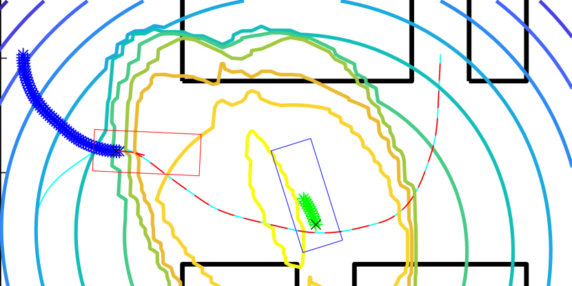
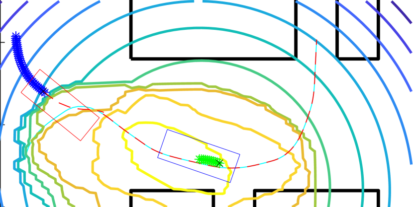
Figure 6: The ego AV following the retreating plans (blue star-lines). The light-blue lines illustrate the original trajectory, the red dashed-lines combining the blue star-lines will be the new reference $\mathcal{P}_{ref}$, and the collision field is illustrated by the contours.

The retreat planner deals with scenarios when stopping or staying on the original reference is deemed unsafe. This can happen when the OV drives toward the ego AV, and its motion largely differs from the previous prediction - possibly violating the safety margin and causing a safety threat. Therefore, the ego AV needs to find a path and retreat from the emergency. The retreating movement is not a standard navigation problem because the ego AV hasn’t had a safe goal. Instead, it needs to explore the environment to find the best goal, and thus we propose a search-based retreat planner which explores the space and quickly finds a retreating trajectory.

As a variant of A*-based algorithms, the retreat planner constructs a tree $\mathcal{T}=(\mathcal{V},\mathcal{E})$ composed of a node set $\mathcal{V}\subset\mathcal{C}_{free}$ and an edge set $\mathcal{E}$, where $E(X_{i},X_{j})\in\mathcal{E}$ represents a feasible short path between $X_{i}$ and $X_{j}$. $\mathcal{C}_{free}$ is implicitly obtained by checking collisions with obstacles in the parking lot map $M_{map}$. Let $\mathcal{M}$ denote a finite set of motion primitives pre-computed through available control actions, and $V_{max}$ denotes the maximum number of nodes allowed. The retreat planner constructs a tree $\mathcal{T}$ from $X_{k}$ (the configuration when the retreat planning starts) and expands it according to a cost function $\mathcal{F}(\cdot)$ which sums up the heuristic value $h(\cdot)$ and the arrival cost $g(\cdot)$. The heuristic (8) is calculated based on a collision field as shown in Fig. 6. The field is a weighted sum of Gaussian distributions centered at waypoints of both the predicted trajectory $\mathbf{X}_{H,k}$, i.e., $X_{h,k}$, and the routes on the cost map, i.e., $X_{m_{k},i}$, and

$$\small h(X)=\sum_{m_{k},i}b(m_{k})e^{-\|X-X_{m_{k},i}\|^{2}_{W_{4}}}+\sum_{h}ce^{-\|X-X_{h,k}\|^{2}_{W_{5}}},$$ (8)

where $c$ is a weighting constant. The planning is completed if the ego AV finds a trajectory that keeps it away from the OV at a safe clearance. If the number of nodes in $\mathcal{T}$ reaches $V_{\max}$, the trajectory giving the maximum clearance is chosen.

III-D3 Trajectory repair planner

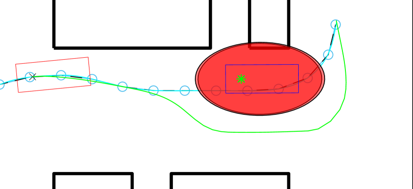
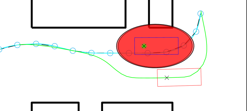
Figure 7: The ego AV (red vehicle) following the repaired plan (green lines) that is calculated from the blocked original trajectory (light-blue lines).

OV’s movements could invalidate the ego AV’s reference trajectory. Fig. 7 illustrates one such case, where an OV, represented by the blue box, stops on the AV’s reference trajectory, represented as the light-blue line. The safety controller will command the ego AV to stop on the reference trajectory when the area in front is infeasible. Unless receiving a new reference trajectory, the safety controller will stop the ego AV and wait for the OV to clear - not efficient if the OV stops for a long time. It is reasonable to update $\mathcal{P}_{ref}$, so that the safety planner can command the ego AV to go around the OV and merge back to the original path. We notice that the repaired trajectory usually lies in the same homotopy class as the original one, which makes an optimization-based repairing strategy a viable solution. To obtain a repaired path quickly, we conduct repair planning over 2D space, i.e., $X_{repair}=[x,y]^{\top}$, and modify the constraints accordingly. It is understood that the resultant path, despite being collision-free, cannot always be followed accurately, causing the AV to collide into obstacles. We therefore verify the path and accept the repaired trajectory (as shown in Fig. 7) only if it passes the kinematic feasibility check. If the repairing fails, the central control will be notified to take over the repairing task.

1 input $M_{map},M_{route},X_{goal}$

2 $\tt{RequestCentralPathPlanning}$$(X_{goal})$

3 while $X_{goal}$ not reached do

4       if $\tt{ReceiveCentralMsg}$ then

5             $\mathcal{P}_{ref}\leftarrow$ $\tt{Update}$$(\mathcal{P}_{ref})$

6            

7      $z_{k}\leftarrow$ $\tt{GetMeasurements}$

8       $X_{cc,k},\mathbf{X}_{H,k},\mathbf{s}_{H,k},b(m_{k}),\hat{m}_{k},bound_{k}\leftarrow$ $\tt{ENVPredict}$$(z_{k},M_{route})$

9       $flag_{retreat}\leftarrow$ $\tt{SafetyCheck}$$(X_{cc,k},s_{k},bound_{k},\hat{m}_{k})$

10       if $flag_{retreat}$ then

11             $\mathcal{P}_{ref}\leftarrow$ $\tt{PlanRetreat}$$(M_{map},M_{route},X_{cc,k},\mathbf{X}_{H,k},b(m_{k}))$

12            

13      $\mathbf{X}_{OV,history}\leftarrow$ $\tt{OV\_MotionHistory}$$(X_{cc,k})$ $flag_{repair}\leftarrow$ $\tt{BlockerCheck}$$(\mathbf{X}_{OV,history},\mathcal{P}_{ref})$

14       if $flag_{repair}$ then

15             $\mathcal{P}_{ref},flag_{fail}\leftarrow$ $\tt{PlanRepair}$$(P_{ref},X_{cc,k})$

16            

17      if $flag_{fail}$ then

18             $\tt{RequestCentralPathPlanning}$$(X_{goal},X_{cc,k})$

19            

20      $\mathbf{X}_{ref,k}\leftarrow$ $\tt{setXref}$$(\mathcal{P}_{ref},\mathbf{X}_{H,k},\mathbf{s}_{H,k},\hat{m}_{k},bound_{k})$

21       $u_{k}\leftarrow$ $\tt{SafetyController}$$(\mathbf{X}_{ref,k},\mathbf{X}_{H,k},\mathbf{s}_{H,k})$

22      

return $u_{k}$

Algorithm 2 The Strategic Motion Planner

IV Empirical Evaluation

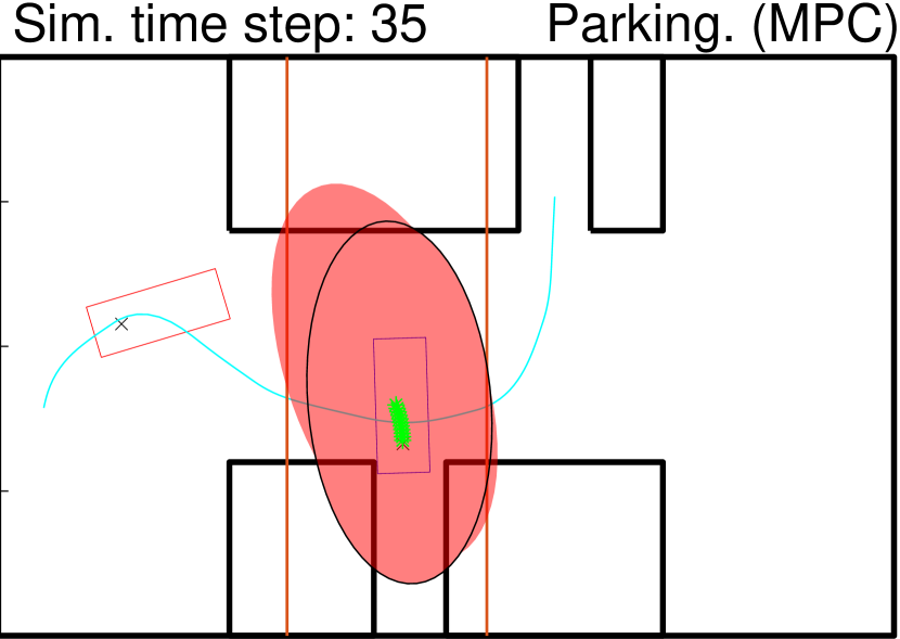
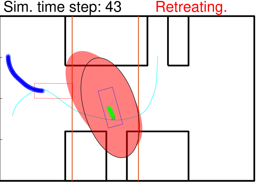
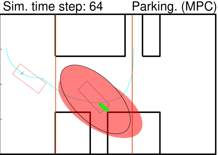
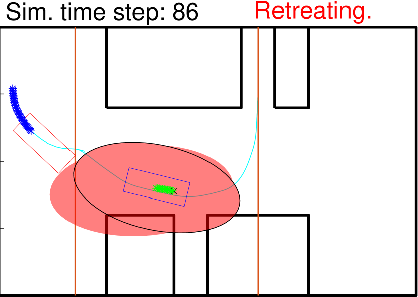
(a)	(b)	(c)	(d)
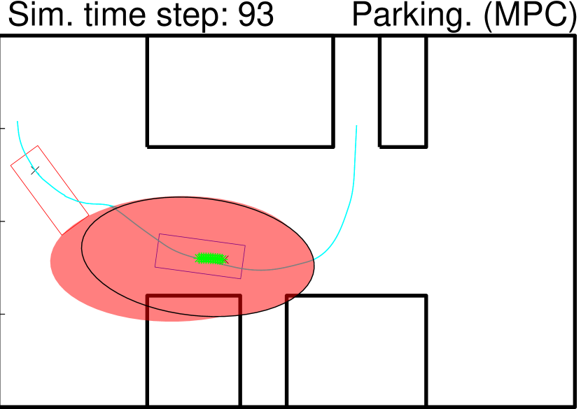
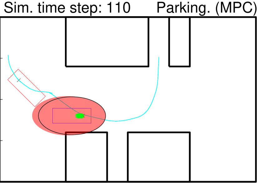
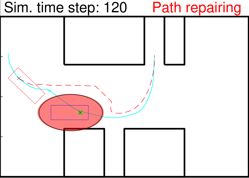
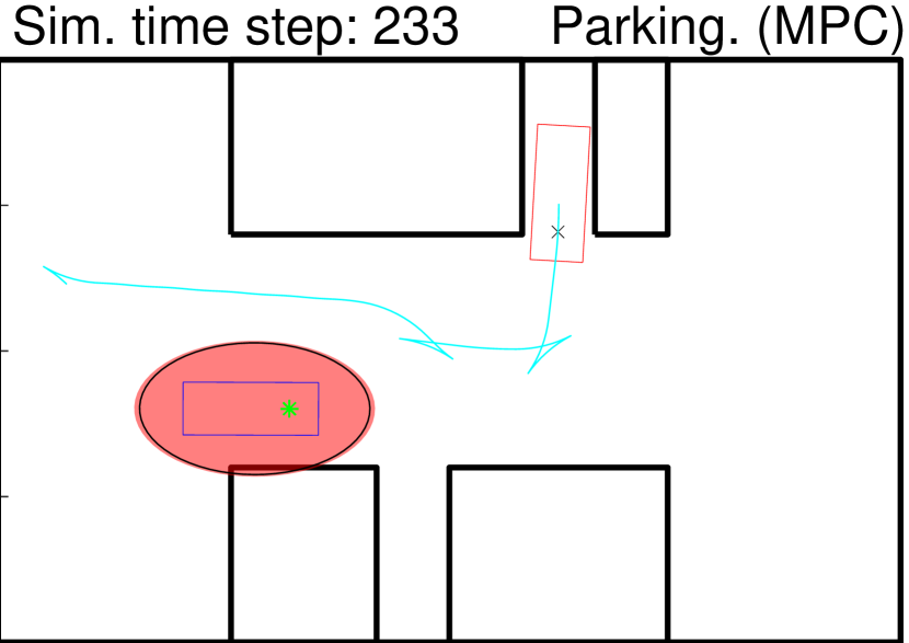
(e)	(f)	(g)	(h)

Figure 8: Simulation results in one of the parking scenarios. (0.25 s/time step)

Figure 9: The simulation result of steering estimation, mode estimation, and safety margin.

The proposed system is tested by simulation, which is conducted on a 6-core Intel i7 3.7GHz desktop with Matlab R2020a. The prediction horizon is $10$, i.e., $H=10$. The integrated system is set to runs at a rate of 4 Hz (all calculation in each time step is finished within 0.1 second). Due to space limitation, this section presents one of the simulation results as an example. More simulation results can be found in the video available at jessicaleu24.github.io/ICRA2022.html.

As shown in Fig. 8(a), the ego AV (red box) first performs parking by tracking the reference trajectory $\mathcal{P}_{ref}$ (light-blue line) while avoiding collision with the OV (blue box). The safety margins are illustrated by red shaded areas, where the one with black edge is for the current time step and the one without edge is for the $Hth$ future time step (the value is shown in Fig. 9). As the OV comes out from its parking spot, it moves towards the ego AV. The ego AV needs to retreat temporarily to make space for the OV (Fig. 8(b)$\sim$(d)). Although the ego AV might be able to avoid collision by backing up along the original reference, this movement may be dangerous since that is the direction where the OV is heading towards and will potentially block the OV. This showcases the importance of considering the long-term mode to construct a collision field (as shown in Fig. 6) of the OV in retreat planning. In Fig. 8(b)-8(c), the retreat planner is activated to update the $\mathcal{P}_{ref}$. When violation happens again (Fig. 8(d)), the retreat planner updates $\mathcal{P}_{ref}$ once more. As the OV completely leaves the parking spot, the estimator detects the mode switch (from ”maneuver left” to ”cruise (exit) left” in Fig. 9), therefore the safety bound is removed (Fig. 8(e)) and the safety controller continues to follow the reference path (Fig. 8(e)-8(f)). Later, the OV stops at the entrance of the road and blocks the original reference trajectory of the ego AV. Therefore, the ego AV tries repairing the trajectory (Fig. 8(g)). However, the repairing fails (the solver converges to an infeasible red path). Because of the narrow space, cusps are required in the maneuver, which is generally hard for an optimization-based planner to generate. Therefore, a new trajectory from the central control is required. Once the updated trajectory $\mathcal{P}_{ref}$ (Fig. 8(h)) is received, the safety controller will start following it until the ego AV reaches the goal. In the video, we show a successful path repair in demo 1 and the effectiveness of the safety bound (so that the retreat planner won’t be triggered unnecessarily) in demo 3.

V Conclusion and Future Work

This paper presents an integrated motion planning strategy for an AV to park in dynamic environments. A hybrid environment predictor incorporates the model-based short-term motion prediction and a driver behavior cost-map to make long-term prediction of an OV. A strategic motion planner, composed of an MPC-based safety controller, a search-based retreating planner, and an optimization-based repairing planner, strikes a good balance between safety, plan feasibility, and smooth maneuver by leveraging the advantages of optimization-based and search-based ideas. Depending on the predictor and the AV’s objective, the strategic motion planner generates safe and smooth trajectories that bring the AV to the target directly or through an intermediate safe spot to yield to OVs. Simulation results demonstrate that the proposed approach enables the ego AV to plan safely and move smoothly in complicated dynamic parking environments. Future work includes: 1) perform rigorous analysis of the integration strategy, e.g., formal method analysis; 2) generalize and verify the proposed strategy in multi-OVs environment; 3) perform real-time simulation in platforms, for instance dSPACE, for comprehensive assessment of performance and computation load.

VI Acknowledgement

The authors would like to thank Karl Berntop, Rien Quirynen, Marcel Menner, and Abraham P. Vinod for their valuable comments.

References

- [1] D. C. Conner, H. Kress-Gazit, H. Choset, A. A. Rizzi, and G. J. Pappas, “Valet parking without a valet,” in 2007 IEEE/RSJ international conference on intelligent robots and systems. IEEE, 2007, pp. 572–577.
- [2] K.-W. Min and J.-D. Choi, “Design and implementation of autonomous vehicle valet parking system,” in 16th International IEEE Conference on Intelligent Transportation Systems (ITSC 2013). IEEE, 2013, pp. 2082–2087.
- [3] J. Leu and M. Tomizuka, “Motion planning for industrial mobile robots with closed-loop stability enhanced prediction,” in Dynamic Systems and Control Conference, vol. 59162. American Society of Mechanical Engineers, 2019, p. V003T19A009.
- [4] D. Ferguson, T. M. Howard, and M. Likhachev, “Motion planning in urban environments: Part ii,” in 2008 IEEE/RSJ International Conference on Intelligent Robots and Systems, 2008, pp. 1070–1076.
- [5] T. Howard, M. Pivtoraiko, R. A. Knepper, and A. Kelly, “Model-predictive motion planning: Several key developments for autonomous mobile robots,” IEEE Robotics Automation Magazine, vol. 21, no. 1, pp. 64–73, 2014.
- [6] D. Dolgov, S. Thrun, M. Montemerlo, and J. Diebel, “Practical search techniques in path planning for autonomous driving,” Ann Arbor, vol. 1001, no. 48105, pp. 18–80, 2008.
- [7] M. McNaughton, C. Urmson, J. M. Dolan, and J.-W. Lee, “Motion planning for autonomous driving with a conformal spatiotemporal lattice,” in 2011 IEEE International Conference on Robotics and Automation. IEEE, 2011, pp. 4889–4895.
- [8] L. Ma, J. Xue, K. Kawabata, J. Zhu, C. Ma, and N. Zheng, “Efficient sampling-based motion planning for on-road autonomous driving,” IEEE Transactions on Intelligent Transportation Systems, vol. 16, no. 4, pp. 1961–1976, 2015.
- [9] F. Islam, V. Narayanan, and M. Likhachev, “A*-connect: Bounded suboptimal bidirectional heuristic search,” in 2016 IEEE International Conference On Robotics and Automation (ICRA). IEEE, 2016, pp. 2752–2758.
- [10] S. Aine, S. Swaminathan, V. Narayanan, V. Hwang, and M. Likhachev, “Multi-heuristic a,” The International Journal of Robotics Research, vol. 35, no. 1-3, pp. 224–243, 2016.
- [11] J. Chen, W. Zhan, and M. Tomizuka, “Constrained iterative lqr for on-road autonomous driving motion planning,” in 2017 IEEE 20th International Conference on Intelligent Transportation Systems (ITSC). IEEE, 2017, pp. 1–7.
- [12] M. F. Hsieh and U. Ozguner, “A parking algorithm for an autonomous vehicle,” in 2008 IEEE Intelligent Vehicles Symposium. IEEE, 2008, pp. 1155–1160.
- [13] R. Kummerle, D. Hahnel, D. Dolgov, S. Thrun, and W. Burgard, “Autonomous driving in a multi-level parking structure,” in 2009 IEEE International Conference on Robotics and Automation. IEEE, 2009, pp. 3395–3400.
- [14] L. Han, Q. H. Do, and S. Mita, “Unified path planner for parking an autonomous vehicle based on rrt,” in 2011 IEEE International Conference on Robotics and Automation. IEEE, 2011, pp. 5622–5627.
- [15] S. Klemm, M. Essinger, J. Oberländer, M. R. Zofka, F. Kuhnt, M. Weber, R. Kohlhaas, A. Kohs, A. Roennau, T. Schamm et al., “Autonomous multi-story navigation for valet parking,” in 2016 IEEE 19th International Conference on Intelligent Transportation Systems (ITSC). IEEE, 2016, pp. 1126–1133.
- [16] Y. Tazaki, H. Okuda, and T. Suzuki, “Parking trajectory planning using multiresolution state roadmaps,” IEEE Transactions on Intelligent Vehicles, vol. 2, no. 4, pp. 298–307, 2017.
- [17] Y. Wang, “Improved a-search guided tree construction for kinodynamic planning,” in 2019 International Conference on Robotics and Automation (ICRA). IEEE, 2019, pp. 5530–5536.
- [18] J. B. Rawlings, D. Q. Mayne, and M. Diehl, Model predictive control: theory, computation, and design. Nob Hill Publishing Madison, WI, 2017, vol. 2.
- [19] R. Schubert, E. Richter, and G. Wanielik, “Comparison and evaluation of advanced motion models for vehicle tracking,” in 2008 11th international conference on information fusion. IEEE, 2008, pp. 1–6.
- [20] A. Houenou, P. Bonnifait, V. Cherfaoui, and W. Yao, “Vehicle trajectory prediction based on motion model and maneuver recognition,” in 2013 IEEE/RSJ international conference on intelligent robots and systems. IEEE, 2013, pp. 4363–4369.
- [21] M. Althoff, O. Stursberg, and M. Buss, “Model-based probabilistic collision detection in autonomous driving,” IEEE Transactions on Intelligent Transportation Systems, vol. 10, no. 2, pp. 299–310, 2009.
- [22] X. Shen, E. L. Zhu, Y. R. Stürz, and F. Borrelli, “Collision avoidance in tightly-constrained environments without coordination: a hierarchical control approach,” arXiv preprint arXiv:2011.00413, 2020.
- [23] J. Schlechtriemen, F. Wirthmueller, A. Wedel, G. Breuel, and K.-D. Kuhnert, “When will it change the lane? a probabilistic regression approach for rarely occurring events,” in 2015 IEEE Intelligent Vehicles Symposium (IV), 2015, pp. 1373–1379.
- [24] X. Shen, I. Batkovic, V. Govindarajan, P. Falcone, T. Darrell, and F. Borrelli, “Parkpredict: Motion and intent prediction of vehicles in parking lots,” in 2020 IEEE Intelligent Vehicles Symposium (IV). IEEE, 2020, pp. 1170–1175.
- [25] N. Deo, A. Rangesh, and M. M. Trivedi, “How would surround vehicles move? a unified framework for maneuver classification and motion prediction,” IEEE Transactions on Intelligent Vehicles, vol. 3, no. 2, pp. 129–140, 2018.
- [26] C. Laugier, I. E. Paromtchik, M. Perrollaz, M. Yong, J.-D. Yoder, C. Tay, K. Mekhnacha, and A. Nègre, “Probabilistic analysis of dynamic scenes and collision risks assessment to improve driving safety,” IEEE Intelligent Transportation Systems Magazine, vol. 3, no. 4, pp. 4–19, 2011.
- [27] S. Lefèvre, D. Vasquez, and C. Laugier, “A survey on motion prediction and risk assessment for intelligent vehicles,” ROBOMECH journal, vol. 1, no. 1, pp. 1–14, 2014.
- [28] Y. Jeong, S. Kim, B. R. Jo, H. Shin, and K. Yi, “Sampling based vehicle motion planning for autonomous valet parking with moving obstacles,” International Journal of Automotive Engineering, vol. 9, no. 4, pp. 215–222, 2018.
- [29] D. A. V. Govea, F. Large, T. Fraichard, and C. Laugier, “Moving obstacles’ motion prediction for autonomous navigation,” in Proc. of the Int. Conf. on Control, Automation, Robotics and Vision, 2004.
- [30] P. E. Hart, N. J. Nilsson, and B. Raphael, “A formal basis for the heuristic determination of minimum cost paths,” IEEE Transactions on Systems Science and Cybernetics, vol. 4, no. 2, pp. 100–107, 1968.
- [31] A. Stentz, “Optimal and efficient path planning for unknown and dynamic environments,” Robotics Institute, Carnegie Mellon University, Tech. Rep. CMU-RI-TR-93-20, 1993.
- [32] M. Likhachev, D. I. Ferguson, G. J. Gordon, A. Stentz, and S. Thrun, “Anytime Dynamic A*: An anytime, replanning algorithm,” in Proc. 2005 ICAPS, 2005, pp. 262–271.
- [33] L. E. Kavraki, P. Svestka, J.-C. Latombe, and M. H. Overmars, “Probabilistic roadmaps for path planning in high-dimensional configuration spaces,” IEEE transactions on Robotics and Automation, vol. 12, no. 4, pp. 566–580, 1996.
- [34] S. M. LaValle and J. J. Kuffner Jr, “Randomized kinodynamic planning,” The international journal of robotics research, vol. 20, no. 5, pp. 378–400, 2001.
- [35] S. Karaman and E. Frazzoli, “Sampling-based algorithms for optimal motion planning,” The international journal of robotics research, vol. 30, no. 7, pp. 846–894, 2011.
- [36] M. Zucker, N. Ratliff, A. D. Dragan, M. Pivtoraiko, M. Klingensmith, C. M. Dellin, J. A. Bagnell, and S. S. Srinivasa, “Chomp: Covariant hamiltonian optimization for motion planning,” The International Journal of Robotics Research, vol. 32, no. 9-10, pp. 1164–1193, 2013.
- [37] J. Schulman, Y. Duan, J. Ho, A. Lee, I. Awwal, H. Bradlow, J. Pan, S. Patil, K. Goldberg, and P. Abbeel, “Motion planning with sequential convex optimization and convex collision checking,” The International Journal of Robotics Research, vol. 33, no. 9, pp. 1251–1270, 2014.
- [38] B. Gutjahr, L. Gröll, and M. Werling, “Lateral vehicle trajectory optimization using constrained linear time-varying mpc,” IEEE Transactions on Intelligent Transportation Systems, vol. 18, no. 6, pp. 1586–1595, 2016.
- [39] X. Zhang, A. Liniger, A. Sakai, and F. Borrelli, “Autonomous parking using optimization-based collision avoidance,” in 2018 IEEE Conference on Decision and Control (CDC). IEEE, 2018, pp. 4327–4332.
- [40] M. Zucker, J. A. Bagnell, C. G. Atkeson, and J. Kuffner, “An optimization approach to rough terrain locomotion,” in 2010 IEEE International Conference on Robotics and Automation. IEEE, 2010, pp. 3589–3595.
- [41] W. Xu, J. Wei, J. M. Dolan, H. Zhao, and H. Zha, “A real-time motion planner with trajectory optimization for autonomous vehicles,” in 2012 IEEE International Conference on Robotics and Automation. IEEE, 2012, pp. 2061–2067.
- [42] S. Dai, M. Orton, S. Schaffert, A. Hofmann, and B. Williams, “Improving trajectory optimization using a roadmap framework,” in 2018 IEEE/RSJ International Conference on Intelligent Robots and Systems (IROS). IEEE, 2018, pp. 8674–8681.
- [43] J. Leu, G. Zhang, L. Sun, and M. Tomizuka, “Efficient robot motion planning via sampling and optimization,” in 2021 American Control Conference (ACC). IEEE, 2021, pp. 4196–4202.
- [44] C. Urmson, J. Anhalt, D. Bagnell, C. Baker, B. Bittner, M. N. Clark, J. Dolan, D. Duggins, T. Galatali, C. Geyer et al., “Autonomous driving in urban environments: Boss and the urban challenge,” Journal of Field Robotics, vol. 25, no. 8, pp. 425–466, 2008.
- [45] M. Montemerlo, J. Becker, S. Bhat, H. Dahlkamp, D. Dolgov, S. Ettinger, D. Haehnel, T. Hilden, G. Hoffmann, B. Huhnke et al., “Junior: The stanford entry in the urban challenge,” Journal of field Robotics, vol. 25, no. 9, pp. 569–597, 2008.
- [46] D. Dolgov, S. Thrun, M. Montemerlo, and J. Diebel, “Path planning for autonomous vehicles in unknown semi-structured environments,” The International Journal of Robotics Research, vol. 29, no. 5, pp. 485–501, 2010.
- [47] C. Chen, M. Rickert, and A. Knoll, “Kinodynamic motion planning with space-time exploration guided heuristic search for car-like robots in dynamic environments,” in 2015 IEEE/RSJ International Conference on Intelligent Robots and Systems (IROS). IEEE, 2015, pp. 2666–2671.
- [48] Z. Ajanovic, B. Lacevic, B. Shyrokau, M. Stolz, and M. Horn, “Search-based optimal motion planning for automated driving,” in 2018 IEEE/RSJ International Conference on Intelligent Robots and Systems (IROS). IEEE, 2018, pp. 4523–4530.
- [49] C. Chen, M. Rickert, and A. Knoll, “Path planning with orientation-aware space exploration guided heuristic search for autonomous parking and maneuvering,” in 2015 IEEE Intelligent Vehicles Symposium (IV). IEEE, 2015, pp. 1148–1153.
- [50] S. Klaudt, A. Zlocki, and L. Eckstein, “A-priori map information and path planning for automated valet-parking,” in 2017 IEEE Intelligent Vehicles Symposium (IV). IEEE, 2017, pp. 1770–1775.
- [51] S. Koenig and M. Likhachev, “D^* lite,” AAAI, vol. 15, 2002.
- [52] X. Sun, W. Yeoh, and S. Koenig, “Moving target d* lite,” in Proceedings of the 9th International Conference on Autonomous Agents and Multiagent Systems: volume 1-Volume 1, 2010, pp. 67–74.
- [53] T. Oral and F. Polat, “Mod* lite: an incremental path planning algorithm taking care of multiple objectives,” IEEE Transactions on Cybernetics, vol. 46, no. 1, pp. 245–257, 2015.
- [54] D. Ferguson, N. Kalra, and A. Stentz, “Replanning with rrts,” in Proceedings 2006 IEEE International Conference on Robotics and Automation, 2006. ICRA 2006. IEEE, 2006, pp. 1243–1248.
- [55] B. Chandler and M. A. Goodrich, “Online rrt* and online fmt*: Rapid replanning with dynamic cost,” in 2017 IEEE/RSJ International Conference on Intelligent Robots and Systems (IROS). IEEE, 2017, pp. 6313–6318.
- [56] O. Adiyatov and H. A. Varol, “A novel rrt*-based algorithm for motion planning in dynamic environments,” in 2017 IEEE International Conference on Mechatronics and Automation (ICMA). IEEE, 2017, pp. 1416–1421.
- [57] J. Qi, H. Yang, and H. Sun, “Mod-rrt*: A sampling-based algorithm for robot path planning in dynamic environment,” IEEE Transactions on Industrial Electronics, 2020.
- [58] W. Ding, W. Gao, K. Wang, and S. Shen, “Trajectory replanning for quadrotors using kinodynamic search and elastic optimization,” in 2018 IEEE International Conference on Robotics and Automation (ICRA). IEEE, 2018, pp. 7595–7602.
- [59] ——, “An efficient b-spline-based kinodynamic replanning framework for quadrotors,” IEEE Transactions on Robotics, vol. 35, no. 6, pp. 1287–1306, 2019.
- [60] X. Zhang, A. Liniger, and F. Borrelli, “Optimization-based collision avoidance,” IEEE Transactions on Control Systems Technology, vol. 29, no. 3, pp. 972–983, 2021.
- [61] J.-H. Jhang and F.-L. Lian, “An autonomous parking system of optimally integrating bidirectional rapidly-exploring random trees* and parking-oriented model predictive control,” IEEE Access, vol. 8, pp. 163 502–163 523, 2020.
- [62] C. Jang, C. Kim, S. Lee, S. Kim, S. Lee, and M. Sunwoo, “Re-plannable automated parking system with a standalone around view monitor for narrow parking lots,” IEEE Transactions on Intelligent Transportation Systems, vol. 21, no. 2, pp. 777–790, 2020.
- [63] M. Hou and R. Patton, “Input observability and input reconstruction,” vol. 34, no. 6, pp. 789–794, Jun. 1998.
- [64] S. Dai and Y. Wang, “Long-horizon motion planning for autonomous vehicle parking incorporating incomplete map information.”
- [65] C. L. Baker, R. Saxe, and J. B. Tenenbaum, “Action understanding as inverse planning,” Cognition, vol. 113, no. 3, pp. 329–349, 2009.
- [66] J. A. E. Andersson, J. Gillis, G. Horn, J. B. Rawlings, and M. Diehl, “CasADi – A software framework for nonlinear optimization and optimal control,” Mathematical Programming Computation, vol. 11, no. 1, pp. 1–36, 2019.