Revealing the Galaxy-Halo Connection Through Machine Learning

Abstract

Understanding the connections between galaxy stellar mass, star formation rate, and dark matter halo mass represents a key goal of the theory of galaxy formation. Cosmological simulations that include hydrodynamics, physical treatments of star formation, feedback from supernovae, and the radiative transfer of ionizing photons can capture the processes relevant for establishing these connections. The complexity of these physics can prove difficult to disentangle and obfuscate how mass-dependent trends in the galaxy population originate. Here, we train a machine learning method called Explainable Boosting Machines (EBMs) to infer how the stellar mass and star formation rate of nearly 6 million galaxies simulated by the Cosmic Reionization on Computers (CROC) project depend on the physical properties of halo mass, the peak circular velocity of the galaxy during its formation history $v_{\mathrm{peak}}$, cosmic environment, and redshift. The resulting EBM models reveal the relative importance of these properties in setting galaxy stellar mass and star formation rate, with $v_{\mathrm{peak}}$ providing the most dominant contribution. Environmental properties provide substantial improvements for modeling the stellar mass and star formation rate in only $\lesssim 10\%$ of the simulated galaxies. We also provide alternative formulations of EBM models that enable low-resolution simulations, which cannot track the interior structure of dark matter halos, to predict the stellar mass and star formation rate of galaxies computed by high-resolution simulations with detailed baryonic physics.

1 Introduction

Numerical simulation enables theoretical models of galaxy formation to include detailed physical models for baryonic processes. Simulations can capture the physics of cooling, supernova feedback, radiative feedback and ionization, and the role of dynamics simultaneously while tracking the growth of cosmological structure formation (e.g., Schaye et al., 2015; Pillepich et al., 2018; Davé et al., 2019). The simulated galaxy populations that result from these models reproduce observed stellar mass sequences such as the main sequence of star-forming galaxies (Brinchmann et al., 2004; Noeske et al., 2007) or the red sequence of quiescent galaxies (Faber et al., 2007). The quest for realism in modeling these observed trends has also added substantial complexity, such that understanding which physical properties of a galaxy most influence its stellar mass and star formation rate can prove challenging. Many theoretical frameworks to describe these relations have been developed (e.g., Wechsler & Tinker, 2018), including halo occupation distribution models (e.g., Jing et al., 1998), subhalo abundance matching (Vale & Ostriker, 2004; Conroy et al., 2006), and semi-analytic models (for a review, see Somerville & Davé, 2015). The complex physics encoded by these models and simulations can be difficult to interpret, and the relative contribution of baryonic feedback, dark matter halo formation, and environment in setting galaxy properties remains challenging to disentangle.

This complexity extends to cosmological models of galaxy formation in the reionization epoch. To capture the distribution of sizes of ionized regions with converged simulations (Iliev et al., 2014) and the largest observed features, such as dark gaps (Zhu et al., 2021), the volume of reionization simulations should extend to a least several hundred megaparsecs. Modeling such large volumes in a single simulation while maintaining the spatial resolution needed to include the complex physics of the current state-of-the-art projects, such as Cosmic Reionization on Computers (CROC Gnedin, 2014), THESAN (Kannan et al., 2021), or Cosmic Dawn (CoDa, Ocvirk et al., 2016, 2020), remains computationally infeasible. Instead, we desire an intermediate approach where large volumes are simulated and the physics of galaxy formation are implemented with a approximate model that recovers the mean trends for galaxy baryonic properties predicted by more detailed calculations. With this goal in mind, a model for reionization sources that encapsulates the results of projects like CROC in a simple module is the first necessary step for deploying lower resolution simulations with much larger ($L\sim 500{\rm cMpc}$) simulation volumes. If the stellar mass and star formation rates of ionizing sources can be predicted from their dark matter halo properties and environment, then we can account for the ionizing photons produced by these sources in large-box simulations of the reionization process without resolving the baryonic physics in detail.

This work employs a machine learning method called Explainable Boosting Machines (EBMs Lou et al., 2013) to infer how stellar mass $M_{\star}$ and star formation rate $S\!F\!R$ depend on the physical parameters $\bm{\theta}$ of a host galaxy. In this work, we use the galaxy populations from the CROC simulations to provide our training and test data that populate samples in the multidimensional parameter space of $M_{\star}$-$S\!F\!R$-$\bm{\theta}$. For the additional parameters $\bm{\theta}$, we use a wide range of physical characteristics measured for galaxies in CROC including the virial mass $M_{\mathrm{vir}}$, redshift $z$, environmental properties averaged on a length scale $R$, and the maximum peak circular velocity $v_{\mathrm{peak}}$. We can then use this approximate machine learning-based EBM model for galaxy formation as a basis for future development to incorporate the CROC galaxy population as sources in lower resolution, large-volume reionization simulations.

EBMs represent a form of Generalized Additive Models (Hastie & Tibshirani, 1986, GAMs) where the dependencies of a target quantity, such as $M_{\star}$ or $S\!F\!R$, on each physical parameter $\theta_{i}$ are encapsulated by feature functions of one parameter (e.g., $f^{i}(\theta_{i})$) or interaction functions of two parameters (e.g., $f^{ij}(\theta_{i},\theta_{j})$). An EBM model is trained to fit these functions from a provided multidimensional dataset. The predicted value of the target quantity given the parameters (e.g., $\gamma(M_{\star}|\bm{\theta})$) is then a sum of the functions $f^{i}$ and $f^{ij}$. EBM models are often described as interpretable because the magnitudes of the functions $f^{i}$ and $f^{ij}$ directly indicate the relative importance of $\bm{\theta}$ in determining the target quantity. If a given parameter $\theta_{i}\!$ is unimportant for determining the target quantity, the EBM will find $f^{i}\!\to\!0$. A formal defintion of the EBM is provided in Section 2.1.

Previous works have applied machine learning models to infer connections between simulated galaxy properties. Lovell et al. (2021) use a tree-based learning method called Extremely Randomized Trees to map baryon information to dark matter halos in the EAGLE simulations. Xu et al. (2021) train a Random Forest to predict the number of central and satellite galaxies in dark matter halos in the Millennium simulation. Machado Poletti Valle et al. (2021) used an XGBoost model to predict gas shapes in dark matter halos in the IllustrisTNG simulations. Bluck et al. (2022) used Random Forest classifiers to study quenching mechanisms in observations, semianalytical models, and cosmological simulations. Piotrowska et al. (2022) also used Random Forest classifiers to examine how supermassive black hole feedback quenches central galaxies in the EAGLE, Illustris, and IllustrisTNG simulations. Our approach complements these prior works by studying the detailed connection between halo and environmental properties, star formation rate, and stellar mass in a model that can be directly implemented in future large-volume cosmological simulations with limited spatial resolution.

The paper is organized as follows. In §2 we review the EBM methodology, define our training dataset and procedure, and introduce the evaluation metrics used to assess the performance of the model. In §3 we present the average contribution of each parameter to the target quantities, the best-fit feature and interaction functions, and the performance of the model in determining the distributions of stellar mass and star formation rate as a function of halo virial mass. We then explore in §4 methods for constructing composite EBM models to recover the stellar mass and star formation rate of simulated galaxies that only use instantaneous halo virial properties and environmental measures (i.e., excluding $v_{\mathrm{peak}}$). We discuss our results in §5, and summarize them and conclude in §6. The Appendicies of the paper provide detailed model results for the EBM for $M_{\star}$ (§A), the mathematical formalism of the composite EBM model (§B), and detailed composite EBM model results for star formation rate (§C) and stellar mass (§D).

2 Methods

To infer the connection between $M_{\star}$, $S\!F\!R$, and other physical properties of simulated galaxies, we apply EBM models to the CROC simulated galaxy catalogs. In §2.1, we define the EBM model. We select our model parameters and describe the simulated galaxy catalog used to train the model in §2.2. The training procedure is outlined in §2.3.

2.1 Explainable Boosting Machines

Explainable Boosting Machine (Lou et al., 2013, EBM) models provide a fitted representation of the relationship between the target quantities $y$ and the parameters $\bm{\theta}$. EBMs are an extension of Generalized Additive Models (Hastie & Tibshirani, 1986, GAMs), which represent target quantities $y$ as the sum of learned univariate functions $f^{i}(\theta_{i})$ that depend on only one parameter $\theta_{i}$. EBMs extend GAMs by including both univariate functions $f^{i}(\theta_{i})$ and bivariate functions $f^{ij}(\theta_{i},\theta_{j})$ that represent dependencies on pairs of features $(\theta_{i},\theta_{j})$ beyond the dependence of the target quantity on either feature independently. Both EBMs and GAMs are forms of regression where the feature functions $f^{i}$ and $f^{ij}$ can be quite general.

The EBM aims to encode the average dependence of a target quantity $y$ on the parameters $\bm{\theta}$. Mathematically, an EBM can therefore be represented as

$$\gamma(y|\bm{\theta})=\beta_{y}+\sum_{i=0}^{n_{\mathrm{p}}-1}f_{y}^{i}(\theta_{i})+\sum_{i=0,i\neq j}^{n_{\mathrm{p}}-1}\sum_{j=0}^{n_{\mathrm{p}}-1}f_{y}^{ij}(\theta_{i},\theta_{j})$$ (1)

where $\gamma(y|\bm{\theta})$ is the predicted value of the target quantity $y$ given $n_{\mathrm{p}}$ parameters $\bm{\theta}\in\mathbb{R}^{n}$ from the dataset. We will refer to learned parameter $\beta_{y}$ as the baseline value of the target quanity $y$. Though $f_{y}^{i}$ and $f_{y}^{ij}$ can be any interpretable function (e.g., linear regression, splines, etc.), Lou et al. (2012) found that gradient boosted trees (Friedman, 2001) work best in practice. Using gradient boosted trees, the functions $f_{y}^{i}$ and $f_{y}^{ij}$ will be piece-wise one- and two-dimensional functions, respectively. By expressing the dependence of $y$ on $\bm{\theta}$ directly through the functions $f_{y}^{i}$ and $f_{y}^{ij}$, EBMs are interpretable and decomposeable. Further, after training is complete the learned tree-based functions $f_{y}^{i}$ and $f_{y}^{ij}$ can be formulated as look-up tables for performant inference.

2.2 Simulated Galaxy Catalog Training Set

To engineer an EBM that describes the connection between simulated galaxy properties, their host dark matter halos, and features of the extrinsic environment, we turn to established observations and theoretical modeling to inform our choices for constructing a training dataset.

The stellar–mass—halo–mass (SHMR) has been directly constrained out to redshifts $z\lesssim 0.05$ and galaxy masses $M_{\rm vir}>10^{12}M_{\odot}$ using galaxy kinematics (e.g. More et al., 2009; Li et al., 2012), $X$-ray observations (e.g Lin et al., 2004; Kravtsov et al., 2018) and gravitational lensing (e.g. Mandelbaum et al., 2005; Velander et al., 2014). These constraints can be extended to higher redshifts ($z<10$) and lower masses ($M_{\rm vir}<10^{10}$) by including halo–galaxy connection modeling (e.g. Nelson et al., 2015; Croton et al., 2016; Rodríguez-Puebla et al., 2017; Behroozi et al., 2019; Girelli et al., 2020). Such models consistently infer that the average stellar mass of galaxies increases with halo mass.

At fixed redshift and halo mass, average galaxy masses of central galaxies differ from satellite galaxies. Halos grow through hierarchical merging, in which small halos merge to form larger halos. As subhalos merge into larger halos, tidal heating and stripping reduce the mass of the more extended dark matter halo, while the satellite galaxy mass remains largely unaffected. For this reason, galaxy mass often correlates better with halo properties at the time of accretion than the current halo mass (e.g. Conroy et al., 2006; Vale & Ostriker, 2006; Moster et al., 2010; Reddick et al., 2013). In particular, SHAM models find that using the halo peak circular velocity, $v_{\rm peak}$, to assign galaxy masss and/or luminosity best reproduces observed galaxy clustering (e.g. Reddick et al., 2013; Hearin et al., 2013; Lehmann et al., 2017).

Star formation rates correlate tightly with galaxy masses, and increase with redshift at fixed stellar mass (e.g. Noeske et al., 2007; Stark et al., 2009; Bouwens et al., 2012). While these trends hold on average, there is a distinct bimodal distribution in the star formation rates of galaxies, corresponding to star-forming and quiescent populations (e.g. Balogh et al., 2004). The observed fraction of quiescent galaxies increases as the Universe evolves (e.g. Tomczak et al., 2014), with the interpretation that some mechanism turns off star formation in galaxies. Many quenching mechanisms have been proposed, including secular/mass quenching (e.g. Kauffmann et al., 2004; Contini et al., 2020) and environmental quenching (e.g. Davies et al., 2016; Trussler et al., 2020). Which of these processes dominate may vary with redshift (Kalita et al., 2021).

Overdense environments may cause environmental quenching, by providing close pairs that can suppress gas accretion (“strangulation”), removing gas through ram-pressure stripping, or disrupting by interactions with other galaxies (“harassment”). Environment thereby influences star formation rates, and low-mass satellite galaxies are typically the most prone to environmental quenching (e.g. Davies et al., 2019).

Given these established trends, galaxy mass and star formation rate may depend on redshift, halo mass, peak circular velocity, and environmental properties. We will therefore select corresponding parameters from the CROC simulated galaxy catalogs to provide our dataset for training the EBM models. Details of the CROC simulations can be found in Gnedin (2014). At a range of redshifts $z$ during the simulation, the computational grid and particle properties are written to disk. These simulation snapshots are post-processed to identify virialized galaxies, as described in Zhu et al. (2020), and the properties of the simulated galaxies are recorded in catalogs. Merger trees are used to identify the properties of simulated galaxies across redshift.

For our target quantities $y$, in this work we will model stellar mass $M_{\star}$ [$h^{-1}M_{\sun}$] and star formation rate $S\!F\!R$ [$M_{\sun}~{}\mathrm{yr}^{-1}$]. The parameters $\bm{\theta}$ selected from the simulated catalog include both intrinsic properties of galaxies and extrinsic properties set by the large scale environment. For intrinsic properties we include the galaxy virial mass $M_{\mathrm{vir}}$ [$h^{-1}M_{\sun}$], the redshift $z$ at which the simulated galaxy properties were measured, and the maximum peak circular velocity $v_{\mathrm{peak}}$ [$\mathrm{km}~{}\mathrm{s}^{-1}$] measured over the formation history of each galaxy. The extrinsic properties used are defined by a length scale $R$ measured relative to each simulated galaxy. We follow convention and substitute $R$ with a numerical value that indicates a number of comoving Mpc (e.g., $\sigma_{8}$ is the rms density fluctuations measured in spheres of radius of $R=8\mathrm{Mpc}$). We compute an environmental density $\rho_{1}\equiv 1+\Delta_{1}$, where $\Delta_{1}$ is the dimensionless matter overdensity measured within 1 $\mathrm{Mpc}$. We include an environmental gas temperature $T_{1}$ [K] averaged on 1 $\mathrm{Mpc}$ scales. From each simulated galaxy we also find the virial mass $M_{\mathrm{max},0.1}$ of the most massive neighboring halo within 100 $\mathrm{kpc}$. We then define the mass ratio $\Upsilon_{0.1}\equiv 1+M_{\mathrm{max},0.1}/M_{\mathrm{vir}}$

The simulated galaxy catalogs include roughly 8,426,327 objects covering a wide range of halo masses, stellar masses, star formation rates, redshifts, and other extrinsic properties. From the catalog of simulated galaxies, objects with a $S\!F\!R<0.001$ $M_{\sun}~{}\mathrm{yr}^{-1}$ were excluded owing to resolution effects artificially limiting their star formation rates. After this culling, the catalog contained 5,950,357 objects that formed our dataset. At this stage, we constructed the training and test datasets from our catalog using the parameter vector $\bm{\theta}=[M_{\mathrm{vir}},z,v_{\mathrm{peak}},\rho_{1},T_{1},\Upsilon_{0.1}]$ to model the target quantities $\bm{y}=[M_{\star},S\!F\!R]$. We use $k$-fold cross-validation (Hastie et al., 2001) with $k=5$, such that the test/training split is 20%/80% for each $k$-folding.

2.3 Training Procedure

The calculations presented in this paper leverage the InterpretML (Nori et al., 2019) implementation of EBMs, using the hyperparameters in Table 1. These InterpretML hyperparameters control the number of bins in the piece-wise $f_{y}^{i}$ and $f_{y}^{ij}$ functions ($\mathcal{Q}_{\mathrm{max}}$, $\mathcal{Q}_{\mathrm{max,2D}}$), the distribution of bins across the fitted domain ($\mathcal{B}$), and the learning rate of the optimization scheme ($\mathcal{R}_{l}$). The Nori et al. (2019) implementation trains an EBM in two phases. First, the univariate functions are optimized using a gradient boosting approach applied round-robin on each parameter, as detailed in Lou et al. (2012). After the univariate functions have converged, the interaction terms are computed and the bivariate functions are optimized according the GA2M/FAST algorithms detailed in Lou et al. (2013). During training we use $k$-fold cross-validation, and merge the training and test datasets for the final performance evaluation of the model.

We evaluate the EBM performance using the mean absolute error (MAE), a variance metric $r^{2}$, and the total outlier fraction $\zeta_{k}$. These statistics provide measures of how well the EBM reproduces the mean trends in the target quantities $y$ as a function of the features $\theta$, the width of the distribution about the mean trends in the training data, and the tails of that distribution.

We calculate the MAE of the model applied to the simulated galaxy sample as

$$\textrm{MAE}=\frac{1}{N}\sum_{i=0}^{N-1}|y_{i}-\hat{y}_{i}|,$$ (2)

where $N$ is the number of objects, $y_{i}$ is the true value of the target quantity for object $i$, and $\hat{y}_{i}$ is the predicted value from the model for object $i$.

We compute the $r^{2}\in[0,1]$ variance metric as

$$r^{2}=1-\frac{\sum_{i=0}^{N-1}(y_{i}-\hat{y}_{i})^{2}}{\sum_{i=0}^{N-1}(y_{i}-\overline{y})^{2}},$$ (3)

which provides a measure of how well the model captures the variance in the data relative to the mean $\overline{y}$, with $r^{2}=1$ reflecting a perfect reproduction of the distribution of $y$ in the training dataset. Note that the feature and interaction functions $f_{y}^{i}$ and $f_{y}^{ij}$ have a finite range, and thus not all values $y_{i}$ can be represented by Equation 1 even when the input parameters $\bm{\theta}$ vary about the mean trends with halo mass or environment. Hence, even for high quality EBM models $r^{2}<1$ and we expect outliers. The $\zeta_{k}$ metric represents the fraction of the total dataset that lies outside the range of predicted values, $\{\hat{y}\}$, as a function of one of the features $\theta_{k}$. We define

$$\zeta_{k}=\frac{1}{N}\sum_{i=0}^{N-1}g_{k,i}(y_{i},\theta_{k,i})$$ (4)

where the index $i$ runs over the total number of samples $N$ and $g_{k,i}(y_{i},\theta_{k,i})$ is a function that returns $1$ if the true target quantity for object $i$ lies outside the predicted range, i.e., $y_{i}\not\in\{\hat{y}\}$. In practice, we compute the outlier fraction for feature $k=\log_{10}M_{\mathrm{vir}}$, and use 2D histograms of ($y_{i}$, $\theta_{k,i}$) and ($\hat{y}_{i}$, $\theta_{k,i}$) to calculate $g_{k,i}$.

In Table 2 we present the evaluation metrics for our EBM model fully trained on the simulated galaxy catalog. For the EBM model for star formation rate ($y=S\!F\!R$), we find a $\mathrm{MAE}\sim 0.14\log_{10}M_{\sun}~{}\mathrm{yr}^{-1}$, a variance metric $r^{2}\sim 0.9$, and an outlier fraction of $<3\%$. For the EBM model for stellar mass ($y=M_{\star}$), we report a $\mathrm{MAE}\sim 0.19\log_{10}M_{\sun}~{}\mathrm{yr}^{-1}$, a variance metric $r^{2}\sim 0.88$, and an outlier fraction of $<1\%$. The good performance of the EBM models in these metrics reflects the abililty of the EBMs to capture both the mean trends and full distributions of the target quantities $y=[M_{\star},S\!F\!R]$ in the training set given the parameters $\bm{\theta}=[M_{\mathrm{vir}},z,v_{\mathrm{peak}},\rho_{1},T_{1},\Upsilon_{0.1}]$. We describe the detailed model results in §3.

EBM Training Hyperparameters
Hyperparameter	Value
Binning $\mathcal{B}$	“uniform”
Maximum Bins, Univariate $\mathcal{Q}_{\mathrm{max}}$	256
Maximum Bins, Bivariate $\mathcal{Q}_{\mathrm{max,2D}}$	$32\times 32$
Learning Rate $\mathcal{R}_{l}$	0.01

Table 1: Hyperparameters used to train the InterpretML (Nori et al., 2019) implementation of the EBM. All other model hyperparameters were set to the default values for InterpretML version 0.2.7.

EBM Training Results
Metrics	$\gamma(S\!F\!R|\bm{\theta})$	$\gamma(M_{\star}|\bm{\theta})$
$r^{2}$	$0.898\pm 0.0003$	$0.882\pm 0.0001$
$\zeta$	$0.029\pm 0.004$	$0.008\pm 0.0010$
	$\log_{10}S\!F\!R$ [$M_{\odot}yr^{-1}$]	$\log_{10}M_{\star}$ [$M_{\odot}$]
MAE	$0.144\pm 0.0001$	$0.189\pm 0.0001$

Table 2: Training results for the EBM using $k$-fold cross validation. See Section 2.3 for more information on the training process. Reported are values for the variance metric $r^{2}$, the outlier fraction $\zeta$, and the mean absolute error (MAE). Uncertainties are computed from the variation among the $k$-fold trials.

3 Results

After training the EBM model to reproduce the dependence of the target quantities $M_{\star}$ and $S\!F\!R$ on the parameters $\bm{\theta}$, the relationships between the target quantities and the parameters can be analyzed. Below, we provide several analyses that quantify how the target quantities relate to the parameters and illustrate the performance of the EBM for our astrophysical applications.

3.1 Average Contribution

A key advantage of using EBM models over “black box” models (e.g., neural networks) is their clear interpretability (see §2.1). The contribution of each parameter $\theta_{i}$ to the model of the target quantity $y$ is provided by the output functions $f_{y}^{i}$ and $f_{y}^{ij}$.

Since these functions are vectors or two-dimensional matrices with a number of elements equal to the number of bins $n_{b}$ in the piece-wise function (see Table 1), a summary scalar quantity for each feature function is helpful for comparing their relative importance. We can define the average contribution $\bar{f}_{y}^{i}$ that provides the average absolute value of $f_{y}^{i}$ or $f_{y}^{ij}$, with the average computed over the number of bins $n_{b}$ and weighted by the number of samples in each bin. Mathematically, we can write

$$\bar{f}_{y}^{i}=\frac{\sum_{j=0}^{n_{b}-1}|f(\theta_{i,j})|N_{j}}{\sum_{j=0}^{n_{b}-1}N_{j}}$$ (5)

where $f$ is the feature function being averaged ($f_{y}^{i}$ or $f_{y}^{ij}$ from Equation 1), $\theta_{i,j}$ is value of the parameter $\theta_{i}$ in the $j$th bin, and $N_{j}$ is the number of samples in bin $j$. Intuitively, the average contribution $\bar{f}_{y}^{i}$ summarizes the importance of each parameter $\theta_{i}$ for determining the target quantities when averaged over the samples in the final, merged dataset.

The average contributions of each feature ($f_{y}^{i}$) or combination of features ($f_{y}^{ij}$) are computed from the EBM. In each case, we rank order the features by decreasing average contribution and focus on the seven features or feature combinations with the largest average contribution. In each case the most important feature has an average contribution more than an order of magnitude larger than the seventh-ranked feature.

3.1.1 EBM Model Targeting Star Formation Rate $S\!F\!R$

Figure 1 shows the average contribution of the top seven features for the EBM model targeting star formation rate $\log_{10}S\!F\!R$. In decreasing order, the seven most important features in determining $S\!F\!R$ are maximum peak circular velocity $v_{\mathrm{peak}}$, virial mass $M_{\mathrm{vir}}$, environmental density $\rho_{1}$, redshift $z$, environmental temperature $T_{1}$, mass ratio of nearby halos $\Upsilon_{0.1}$, and the interaction between $M_{\mathrm{vir}}$ and $\Upsilon_{0.1}$. The numerical values for the average contributions are provided in Table 3. The baseline value of $S\!F\!R$ is $\beta_{\log_{10}S\!F\!R}=-2.1151~{}[\log_{10}M_{\sun}~{}\mathrm{yr}^{-1}]$, typical of halos with $\log_{10}M_{\mathrm{vir}}\sim 9$. The average contribution of $v_{\mathrm{peak}}$ and $M_{\mathrm{vir}}$ are quite similar, providing $\Delta\log_{10}S\!F\!R>0.2$ on average, but their interaction term is small with $\bar{f}(\log_{10}v_{\mathrm{peak}},\log_{10}M_{\mathrm{vir}})\ll 0.01$. Therefore peak circular velocity and virial mass provide important contributions to determining the star formation rate, and the univariate dependence of the $S\!F\!R$ on these properties accounts for most of their contribution. At the few-percent level, environmental density, redshift, environmental gas temperature, and the presence of nearby massive halos also contribute.

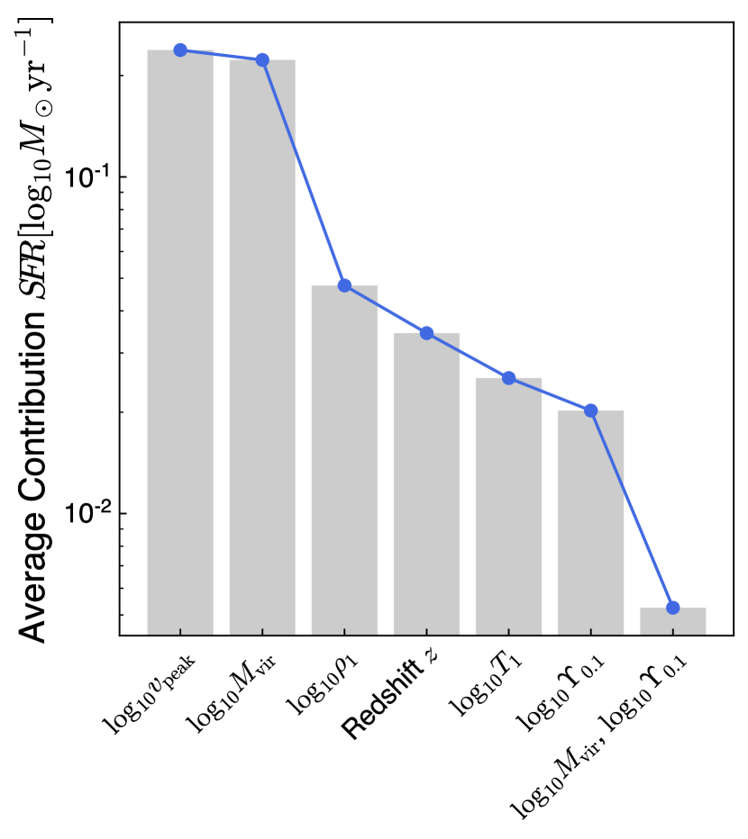
Figure 1: Top seven features with the highest average contribution in the EBM $\gamma(S\!F\!R|\bm{\theta})$ targeting the star formation rate $S\!F\!R$. In order of decreasing importance, these features include peak circular velocity $v_{\mathrm{peak}}$, virial mass $M_{\mathrm{vir}}$, environmental density $\rho_{1}$, redshift $z$, environmental temperature $T_{1}$, the mass ratio of nearby halos $\Upsilon_{0.1}$, and the interaction between virial mass $M_{\mathrm{vir}}$ and $\Upsilon_{0.1}$. Average contribution is calculated using the average of the absolute value of the feature functions weighted by the number of samples in each bin (see Equation 5).

Average Contributions for the $\gamma(M_{\star}|\bm{\theta})$ EBM
Feature	Value [$\log_{10}M_{\sun}~{}\mathrm{yr}^{-1}$]
$\beta_{\log_{10}M_{\star}}$	$-2.1151$
$\bar{f}(\log_{10}v_{\mathrm{peak}})$	$0.2380$
$\bar{f}(\log_{10}M_{\mathrm{vir}})$	$0.2224$
$\bar{f}(\log_{10}\rho_{1})$	$0.0475$
$\bar{f}(z)$	$0.0343$
$\bar{f}(\log_{10}T_{1})$	$0.0252$
$\bar{f}(\log_{10}\Upsilon_{0.1})$	$0.0202$
$\bar{f}(\log_{10}M_{\mathrm{vir}},\log_{10}\Upsilon_{0.1})$	$0.0052$

Table 3: Summary of the EBM model trained to predict $S\!F\!R$. The first entry, $\beta_{\log_{10}S\!F\!R}$, is the baseline value learned model (see Section 2.1). The next seven entries are the average contributions of the most important feature functions listed in descending order (see Equation 5).

The feature functions $f_{y}^{i}$ for each feature are plotted in Figure 2. The functions indicate that there are positive correlations between the star formation rate $\log_{10}S\!F\!R$ and either the peak circular velocity $v_{\mathrm{peak}}$, virial mass $M_{\mathrm{vir}}$, or environmental density $\rho_{1}$. The star formation rate increases with increasing environmental temperature $\log_{10}T_{1}$, but near $T_{1}\approx 10^{4}$K the univariate function shows an enhancement just as hydrogen becomes mostly neutral and a deficit near the temperature at which it becomes ionized. Star formation rate increases with decreasing redshift over the range $z\sim 5-15$, becoming more efficient after reionization.

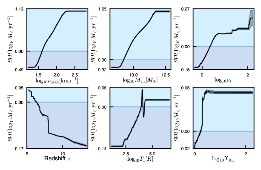
Figure 2: Learned univariate feature functions $f_{y}^{i}$ for the EBM $\gamma(S\!F\!R|\bm{\theta})$ trained to predict the star formation rate $S\!F\!R$. Shown (left to right) are the feature functions for peak circular velocity $v_{\mathrm{peak}}$, virial mass $M_{\mathrm{vir}}$, environmental density $\rho_{1}$, redshift $z$, environmental temperature $T_{1}$, and nearby halo mass ratio $\Upsilon_{0.1}$. Light blue areas indicate regions where $f_{y}^{i}>0$ and dark blue areas indicate regions where $f_{y}^{i}<0$. The shaded areas show the variation in $f_{y}^{i}$ between the $k$-fold iterations.

The interaction functions $f_{y}^{ij}$ learned by the EBM $\gamma(S\!F\!R|\bm{\theta})$ targeting the star formation rate $S\!F\!R$ are plotted as “heat maps” in Figure 3. Most interaction functions do not contribute significantly to the star formation rate, and change the star formation rate by $\Delta\log_{10}S\!F\!R\lesssim 0.05$. However, halos with low neighboring halo mass ratios $\Upsilon_{0.1}$ and large peak circular velocity $v_{\mathrm{peak}}$ have their star formation rate enhanced by $\Delta\log_{10}S\!F\!R\approx 0.15$. Rephrased, locally dominant halos with large peak circular velocity show enhanced star formation. Such enhancements likely owe to recent merger activity.

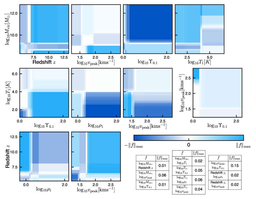
Figure 3: Most important learned interaction functions $f_{y}^{ij}$ for the EBM model $\gamma(S\!F\!R|\bm{\theta})$ targeting the star formation rate $S\!F\!R$, as a function of their parameter pairs. Each panel shows the contribution of the bivariate interaction terms, normalized such that the color map ranges between plus or minus the maximum of the norm of each function $||f||_{\mathrm{max}}$. Light blue areas indicate regions of joint parameter space where the feature interactions contribute positively to the star formation rate, while dark blue areas indicate regions with negative contributions. The table lists $||f||_{\mathrm{max}}$ for the interaction functions, each with units $\log_{10}M_{\sun}~{}\mathrm{yr}^{-1}$. In absolute terms, the largest interaction occurs for halos with large peak circular velocity $v_{\mathrm{peak}}$ and no large neighboring halos ($\Upsilon_{0.1}\approx 0$). The other interaction functions are relatively weak, and contribute changes to $\log S\!F\!R\lesssim 0.05$.

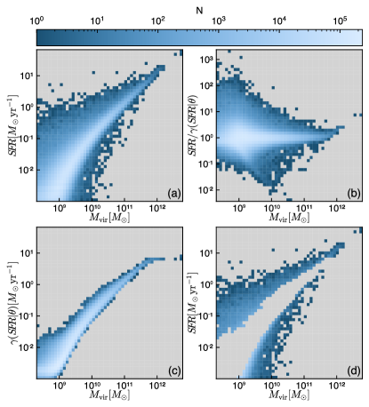
Figure 4: Summary of the EBM model $\gamma(S\!F\!R|\bm{\theta})$ targeting star formation rate ($S\!F\!R$) as a function of virial mass. The upper left panel shows the two-dimensional distribution of $S\!F\!R$ with $M_{\mathrm{vir}}$ for galaxies in the CROC simulations, with the color scale showing the number of simulated galaxies at each $[S\!F\!R,M_{\mathrm{vir}}]$ location. The lower left panel shows the EBM model results for the distribution of $S\!F\!R$ with $M_{\mathrm{vir}}$, where the $S\!F\!R$ is computed from the EBM using the parameters $\bm{\theta}=[M_{\mathrm{vir}},v_{\mathrm{peak}},z,\rho_{1},T_{1},\Upsilon_{0.1}]$. The upper right panel shows the residuals between the simulated CROC galaxy $S\!F\!R$s and the EBM model results. The lower right panel shows the simulated CROC galaxy $S\!F\!R$s that lie outside the EBM model predictions. These outliers represent $\lesssim 3\%$ of simulated CROC galaxies.

While Equation 1 represents a complex, multidimensional manifold that provides the $S\!F\!R$ as a function of the parameters $\bm{\theta}$, the distributions of simulated and predicted $S\!F\!R$ as a function of a single parameter provide a graphical summary of the EBM model performance. Figure 4 shows the simulated and predicted $S\!F\!R$ as a function of virial mass $\log_{10}M_{\mathrm{vir}}$, and we will refer to this figure as the model summary. Shown in this model summary are the distributions of $S\!F\!R$ in the CROC simulated galaxy catalogs with virial mass and the $S\!F\!R$ predicted by the EBM model $\gamma(S\!F\!R|\bm{\theta})$ using the parameters $\bm{\theta}$ measured for each simulated galaxy. The EBM model captures roughly 97% of the simulated distribution of $S\!F\!R$ with virial mass. The EBM model is highly predictive of the simulated connection between $S\!F\!R$ and the intrinsic and extrinsic properties $\bm{\theta}$.

Given the combined complexity of the average contribution measures, univariate feature functions, and bivariate interaction functions, in what follows we will show the summary figure for other EBM models in the main text. For completeness, the average contribution, feature function, and interaction function figures for each model will be presented in the Appendices.

3.1.2 EBM Model Targeting Stellar Mass $M_{\star}$

An EBM model $\gamma(M_{\star}|\bm{\theta})$ targeting stellar mass $M_{\star}$ using the properties $\bm{\theta}$ can be constructed through simple retraining. Using the simulated galaxy catalogs from CROC, we retrain the EBM to model $M_{\star}$ against $\bm{\theta}$. We report the average contribution, univariate feature functions, and bivariate interaction functions for $\gamma(M_{\star}|\bm{\theta})$ in Appendix A. For reference, the baseline value of $M_{\star}$ is $\beta_{\log_{10}M_{\star}}=5.9629~{}[\log_{10}M_{\sun}~{}\mathrm{yr}^{-1}]$ (see Table 6 in the Appendix), typical of halos with $\log_{10}M_{\mathrm{vir}}/M_{\sun}\sim 9$.

Figure 5 shows the model summary for the EBM model $\gamma(M_{\star}|\bm{\theta})$. The EBM model provides an excellent representation of the distribution of stellar masses for the CROC simulated galaxy catalog. As the lower right panel of Figure 5 indicates, the $\gamma(M_{\star}|\bm{\theta})$ model results in few outliers for the CROC simulated galaxies and has an outlier fraction of $\lesssim 1\%$. Given the galaxy properties $\bm{\theta}=[M_{\mathrm{vir}},z,v_{\mathrm{peak}},\rho_{1},T_{1},\Upsilon_{0.1}]$, the distribution of stellar masses for CROC simulated galaxies can be recovered to 99% accuracy.

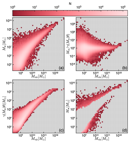
Figure 5: Summary of the EBM model $\gamma(M_{\star}|\bm{\theta})$ targeting stellar mass $M_{\star}$ as a function of virial mass. The upper left panel shows the distribution of $M_{\star}$ with virial mass $M_{\mathrm{vir}}$ in the CROC simulated galaxy catalogs, with the coloration indicating the number of galaxies at each $[M_{\star},M_{\mathrm{vir}}]$ location. The lower left panel shows the EBM model prediction of the stellar mass distribution with virial mass given in the input parameters $\bm{\theta}=[M_{\mathrm{vir}},z,v_{\mathrm{peak}},\rho_{1},T_{1},\Upsilon_{0.1}]$. The upper right panel shows the residuals between the simulated and predicted $M_{\star}$ vs. $M_{\mathrm{vir}}$ distribution, and the lower right panel shows the outliers in the simulated distribution not captured by the EBM model $\gamma(M_{\star}|\bm{\theta})$. The fraction of outliers is $\lesssim 1\%$.

4 Composite EBMs for Restricted Parameter Sets

The EBM models $\gamma(S\!F\!R|\bm{\theta})$ and $\gamma(M_{\star}|\bm{\theta})$ presented in §3.1.1 and §3.1.2 are constructed using the parameter set $\bm{\theta}=[M_{\mathrm{vir}},z,v_{\mathrm{peak}},\rho_{1},T_{1},\Upsilon_{0.1}]$. Our results show that the full distribution of $S\!F\!R$ and stellar mass in the simulated CROC galaxy catalogs can be recovered accurately with only $\approx 1-3\%$ outliers. These EBM models can therefore be applied to cosmological simulations using the parameters $\bm{\theta}$ measured from simulated galaxy catalogs to recover the distribution of $S\!F\!R$ and stellar mass computed by CROC.

The parameters $\bm{\theta}$ include the peak circular velocity $v_{\mathrm{peak}}$, which requires both time-dependent tracking of formation histories for individual galaxies and high spatial resolution to capture the peak of the rotation curve for each object. As a result, as expressed above the models $\gamma(S\!F\!R|\bm{\theta})$ and $\gamma(M_{\star}|\bm{\theta})$ cannot be applied directly to cosmological simulations with low spatial resolution or without merger trees to capture formation histories.

Instead of fitting EBM models using the full parameter set $\bm{\theta}$, consider the construction of an EBM model using the restricted parameter set $\bm{\theta}^{\prime}=[M_{\mathrm{vir}},z,\rho_{1},T_{1},\Upsilon_{0.1}]$ that does not include $v_{\mathrm{peak}}$. The parameters $\bm{\theta}^{\prime}$ can all be measured directly in cosmological simulations with sufficient resolution to capture individual galaxy-mass halos without the need to track merger trees. The EBM models $\gamma(S\!F\!R|\bm{\theta}^{\prime})$ and $\gamma(M_{\star}|\bm{\theta}^{\prime})$ using the restricted parameter set $\bm{\theta}^{\prime}$ perform substantially less well than the models $\gamma(S\!F\!R|\bm{\theta})$ and $\gamma(M_{\star}|\bm{\theta})$ trained on the full parameter set $\bm{\theta}$ that includes $v_{\mathrm{peak}}$. With the restricted parameter set $\bm{\theta}^{\prime}$, the EBM model shows $7.6\%$ outliers when targeting $S\!F\!R$ and $2.8\%$ when targeting $M_{\star}$. Comparing with the outlier fractions reported in Table 2 for the full parameter set including $v_{\mathrm{peak}}$, the EBM model trained on the restricted dataset has degraded its performance by a factor of $\sim 2-3$.

To ameliorate the poorer performance of the EBM models trained on restricted parameter sets, we use a Composite EBM (CEBM) model. Given a target quantity $y$ and a parameter set $\bm{\theta}^{\prime}$, we fit a base EBM $\gamma(y|\bm{\theta}^{\prime})$ in the same manner as fitting the EBMs $\gamma(S\!F\!R|\bm{\theta})$ or $\gamma(M_{\star}|\bm{\theta})$. We construct a dataset from the galaxies whose $y$ values lie outside the predictions from $\gamma(y|\bm{\theta}^{\prime})$, and then fit an outlier EBM $\delta(y|\bm{\theta}^{\prime})$ to these discrepant samples. We then weight the base and outlier EBMs to construct the CEBM model $\Gamma(M_{\star}|\bm{\theta}^{\prime})$ using a classifier EBM $\phi_{y}(\bm{\theta}^{\prime})$. Instead of fitting the change in star formation rate or stellar mass at a given sample in $\theta^{\prime}$, the classifier EBM fits the log odds that a given sample in $\theta^{\prime}$ is an outlier. We then define $\phi_{y}(\bm{\theta}^{\prime})$ to be the sigmoid of these log odds, such that $\phi_{y}(\bm{\theta}^{\prime})\in[0,1]$. The CEBM can then be written as

$$\Gamma(M_{\star}|\bm{\theta}^{\prime})=[1-\phi_{y}(\bm{\theta}^{\prime})]\gamma(y|\bm{\theta}^{\prime})+\phi_{y}(\bm{\theta}^{\prime})\delta(y|\bm{\theta}^{\prime}).$$ (6)

We describe the CEBM approach in more detail in Appendix B, and provide information on the CEBMs $\Gamma(S\!F\!R|\bm{\theta}^{\prime})$ and $\Gamma(M_{\star}|\bm{\theta}^{\prime})$ in Appendices C and D.

Table 4 lists the evaluation metrics for the training of CEBM models targeting $S\!F\!R$ and stellar mass without using $v_{\mathrm{peak}}$. The outlier fraction has improved to $\approx 5\%$ for CEBM model $\Gamma(S\!F\!R|\bm{\theta}^{\prime})$ and to $\lesssim 2\%$ for $\Gamma(M_{\star}|\bm{\theta}^{\prime})$. The average parameter contributions and baseline value $\beta_{\log_{10}S\!F\!R}$ from $\Gamma(S\!F\!R|\bm{\theta}^{\prime})$ are provided in Table 5 and for the CEBM targeting stellar mass in Table 7. The univariate feature functions and bivariate interaction functions for the CEBM models $\Gamma(S\!F\!R|\bm{\theta}^{\prime})$ and $\Gamma(M_{\star}|\bm{\theta}^{\prime})$ are provided in Appendices C and D.

Figure 6 shows the model summary for the CEBM targeting $S\!F\!R$, and Figure 7 shows the model summary for the CEBM targeting stellar mass. As both models demonstrate, the CEBM model accurately recovers the distribution of star formation rate and stellar mass in the CROC simulated galaxy sample. Between the models, the outlier fraction is only $\approx 2-5\%$ despite using the restricted set of parameters $\bm{\theta}^{\prime}$ that does not include $v_{\mathrm{peak}}$ or any time-dependent tracking of individual systems.

Composite EBM Training Results
Metrics	$\gamma(S\!F\!R|\bm{\theta})$	$\gamma(M_{\star}|\bm{\theta})$
$r^{2}$	$0.868\pm 0.0002$	$0.830\pm 0.0003$
$\zeta$	$0.052\pm 0.0053$	$0.018\pm 0.0031$
	$\log_{10}S\!F\!R$ [$M_{\odot}yr^{-1}$]	$\log_{10}M_{\star}$ [$M_{\odot}$]
MAE	$0.165\pm 0.0001$	$0.233\pm 0.0002$

Table 4: Training results for CEBM models for $S\!F\!R$ and $M_{\star}$ using $k$-fold cross validation. See Section 2.3 for more information on the training process. Reported are values for the variance metric $r^{2}$, the outlier fraction $\zeta$, and the mean absolute error (MAE). Uncertainties are computed from the variation among the $k$-fold trials.

Overview of CEBM $\Gamma(S\!F\!R|\bm{\theta}^{\prime})$
Feature	Value [$\log_{10}M_{\sun}~{}\mathrm{yr}^{-1}$]
$\beta_{\log_{10}S\!F\!R}$	$-1.7466$
$\tilde{f}(\log_{10}M_{\mathrm{vir}})$	$0.4327$
$\tilde{f}(\log_{10}\rho_{1})$	$0.0625$
$\tilde{f}(\log_{10}T_{1})$	$0.0327$
$\tilde{f}(\log_{10}\Upsilon_{0.1})$	$0.0215$
$\tilde{f}(z)$	$0.0190$
$\tilde{f}(z,\log_{10}\rho_{1})$	$0.0077$
$\tilde{f}(\log_{10}M_{\mathrm{vir}},\log_{10}\Upsilon_{0.1})$	$0.0056$

Table 5: Average contribution to the CEBM model $\Gamma(S\!F\!R|\bm{\theta}^{\prime})$ trained to predict $S\!F\!R$ from the parameter set $\bm{\theta}^{\prime}$. The first entry, $\beta_{\log_{10}S\!F\!R}$, is the learned baseline of the model. The next seven entries are the feature functions with the highest average contribution listed in descending order. The average contribution is calculated using the average of the absolute value of the base EBM function values weighted by the number of samples in each bin and the output of the classification EBM for each sample (see Appendix B.2 for more details).

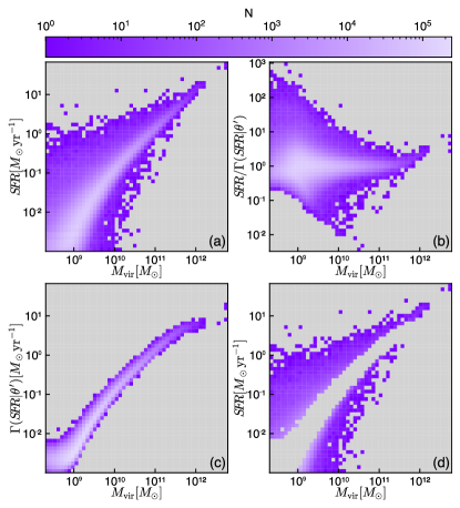
Figure 6: Summary of the CEBM model $\Gamma(S\!F\!R|\bm{\theta}^{\prime})$ targeting star formation rate ($S\!F\!R$) as a function of virial mass. The upper left panel shows the two-dimensional distribution of $S\!F\!R$ with $M_{\mathrm{vir}}$ for galaxies in the CROC simulations, with the color scale showing the number of simulated galaxies at each $[S\!F\!R,M_{\mathrm{vir}}]$ location. The lower left panel shows the CEBM model results for the distribution of $S\!F\!R$ with $M_{\mathrm{vir}}$, where the $S\!F\!R$ is computed from the CEBM using the parameters $\bm{\theta}^{\prime}=[M_{\mathrm{vir}},z,\rho_{1},T_{1},\Upsilon_{0.1}]$. The upper right panel shows the residuals between the simulated CROC galaxy $S\!F\!R$s and the CEBM model results. The lower right panel shows the simulated CROC galaxy $S\!F\!R$s that lie outside the CEBM model predictions. These outliers represent $\approx 5\%$ of simulated CROC galaxies.

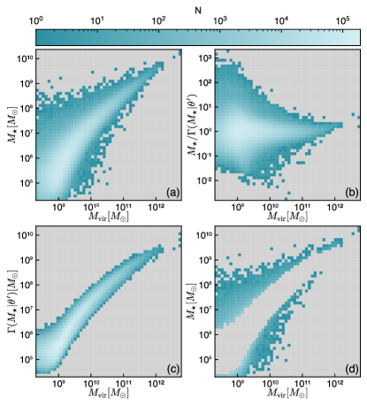
Figure 7: Summary of the CEBM model $\Gamma(M_{\star}|\bm{\theta}^{\prime})$ targeting stellar mass $M_{\star}$ as a function of virial mass. The upper left panel shows the distribution of $M_{\star}$ with virial mass $M_{\mathrm{vir}}$ in the CROC simulated galaxy catalogs, with the coloration indicating the number of galaxies at each $[M_{\star},M_{\mathrm{vir}}]$ location. The lower left panel shows the CEBM model prediction of the stellar mass distribution with virial mass given in the input parameters $\bm{\theta}^{\prime}=[M_{\mathrm{vir}},z,\rho_{1},T_{1},\Upsilon_{0.1}]$. The upper right panel shows the residuals between the simulated and predicted $M_{\star}$ vs. $M_{\mathrm{vir}}$ distribution, and the lower right panel shows the outliers in the simulated distribution not captured by the CEBM model $\Gamma(M_{\star}|\bm{\theta}^{\prime})$. The fraction of outliers is $\lesssim 2\%$.

5 Discussion

Explainable Boosting Machine (EBM) models provide a method to statistically infer relationships present in high-dimensional data. Given their statistical nature, EBM models remain ignorant of the physics that generate the connection between star formation rate, stellar mass, and the properties of dark matter halos that host galaxies. Nonetheless, given the results of detailed physical modeling in the form of simulated galaxy catalogs from cosmological simulations, the EBM correctly identifies halo mass and maximum peak circular velocity as the most important halo properties for determining $S\!F\!R$ and $M_{\star}$ (e.g., Figure 1). The EBM correctly infers that $S\!F\!R$ and $M_{\star}$ increase with increasing halo mass or $v_{\mathrm{peak}}$, and the EBM univariate feature functions correctly identify the gas temperature at which star formation efficiency changes. To the extent that the physical connection between galaxy and halo properties are recorded in statistical relationships, the EBM models effectively recover some fraction of those relations.

EBM models also provide a means to implement a “sub-grid” prescription for galaxy formation based on the properties of halos and their environments. The EBM models $\gamma(S\!F\!R|\bm{\theta})$ and $\gamma(M_{\star}|\bm{\theta})$ capture better than 97% of the $S\!F\!R$ and $M_{\star}$ distributions measured for simulated galaxies in the CROC simulations. The stellar masses and star formation rates of galaxies in CROC could be accurately recovered by using only the halo and environmental parameters in $\bm{\theta}=[M_{\mathrm{vir}},z,v_{\mathrm{peak}},\rho_{1},T_{1},\Upsilon_{0.1}]$.

Using the CEBM model trained on the restricted parameter set $\bm{\theta}^{\prime}=[M_{\mathrm{vir}},z,\rho_{1},T_{1},\Upsilon_{0.1}]$, $\approx 95-98\%$ of the distribution of $S\!F\!R$ and $M_{\star}$ of the CROC galaxies is recovered. One advantage of this parameter set is that the spatial resolution in the simulations required to compute them is less demanding than for $v_{\mathrm{peak}}$. A simulation with coarser resolution than CROC, such that the details of the star formation and feedback processes cannot be resolved, may still leverage the CEBM models $\Gamma(S\!F\!R|\bm{\theta}^{\prime})$ and $\Gamma(M_{\star}|\bm{\theta}^{\prime})$ to model the star formation rate and stellar masses in dark matter halos. Further, the quantities $\bm{\theta}^{\prime}$ used to train the CEBM models are measured at distinct redshifts such that no merger trees are required to recover accurately the CROC $S\!F\!R$ and $M_{\star}$ distributions from halo and environmental properties. We note that for both the EBM and CEBM models the outlier fractions not well captured by the model are roughtly percent-level or less in the $S\!F\!R$ or $M_{\star}$ distributions, and we expect that corresponding inaccuracies induced in, e.g., the ionizing photon budget or topology of reionization will be minimal.

By editing the dataset and retraining, the impact of environment on the performance of the EBM models can be estimated. Relative to $\gamma(S\!F\!R|\bm{\theta})$ and $\gamma(M_{\star}|\bm{\theta})$ that use the full dataset $\bm{\theta}$ including all environmental parameters, EBM models trained only on maximum peak circular velocity $v_{\mathrm{peak}}$, halo virial mass $M_{\mathrm{vir}}$, and redshift $z$ have an outlier fraction increased by only $\sim 1\%$ when modeling $M_{\star}$ and $\sim 10\%$ when modeling $S\!F\!R$. Further, removing $v_{\mathrm{peak}}$ and training only on $[M_{\mathrm{vir}},z]$ substantially degrades the model performance, and the outlier fractions increase to $\sim 20\%$ when modeling $M_{\star}$ and $\sim 40\%$ when modeling $S\!F\!R$. The importance of including $v_{\mathrm{peak}}$ in the training dataset is much larger than the importance of accounting for the environmental measures selected in this analysis.

The EBM models enable an approximate translation of the galaxy formation model from one simulation to another. Provided the parameter sets $\bm{\theta}$ or $\bm{\theta}^{\prime}$ can be measured in both simulations, an EBM can recover the connection between $S\!F\!R$, stellar masses, halo properties, and environment from the training simulation and then be used to instill those relations in a different simulation. Since the $\bm{\theta}^{\prime}$ parameter set does not require very high spatial resolution to capture, the net results for $S\!F\!R$ and stellar mass from a high resolution simulation accurately tracking detailed baryonic physics can be translated into a simulation with resolution insufficient to capture those physics directly. In future work, we plan to transfer the CROC baryonic galaxy formation model into Cholla cosmological simulations (e.g., Villasenor et al., 2021a, b) via the EBM models presented here. Such a transferred model could be used to build models of feedback from galaxy formation on resolved scales that incorporate the regulatory effects of feedback on small-scale star formation.

Lastly, the ability of the EBM models to recover the $S\!F\!R$ and $M_{\star}$ distributions using only halo and environmental properties allows for the rapid replacement of galaxy formation models based on EBMs. Models can be trained on the simulated galaxy catalogs from a variety of expensive, high-resolution training simulations including a wide range of physics. These EBM models can then be used interchangeably as effective galaxy formation models in the target simulations, and can also be modified posteriori to allow a broad parameter search or correct the inaccuracies of the training simulation. Such an approach could reduce the sensitivity of conclusions about, e.g., the reionization process on the detailed $S\!F\!R$ and $M_{\star}$ distributions as multiple EBM models for these properties could be trained and implemented in the target simulations.

6 Summary

A complex interplay of physical processes gives rise to the distribution of star formation rates ($S\!F\!R$s) and stellar masses $M_{\star}$ of galaxies over cosmic time. Cosmological simulations provide powerful methods for modeling these physical processes, but the connection between $S\!F\!R$, $M_{\star}$, and other galaxy properties can be obfuscated by complexity. Leveraging machine learning techniques, we use a variation of the Generalized Additive Model (Hastie & Tibshirani, 1986) called Explainable Boosting Machines (EBM Nori et al., 2019) to infer the dependence of $S\!F\!R$ and $M_{\star}$ in the Cosmic Reionization on Computers (CROC) simulations (Gnedin, 2014) on dark matter halo properties including virial mass $M_{\mathrm{vir}}$, peak maximum circular velocity $v_{\mathrm{peak}}$, redshift, environmental density, environmental gas temperature, and the mass of neighboring halos. Our findings include:

• $S\!F\!R$ and $M_{\star}$ primarily depend on $M_{\mathrm{vir}}$ and $v_{\mathrm{peak}}$, followed by redshift, environmental density, and environmental gas temperature.

• When including $M_{\mathrm{vir}}$ and $v_{\mathrm{peak}}$ in the parameter set used to train the EBM, the model recovers better than 97% of the distribution of $M_{\star}$ or $S\!F\!R$ with virial mass $M_{\mathrm{vir}}$ in the CROC simulations.

• If the model fit excludes $v_{\mathrm{peak}}$, the fraction of outliers in the CROC data relative to the predicted model distribution increases to 7.6% for $S\!F\!R$ and 2.8% for $M_{\star}$.

• To ameliorate the degradation of the model performance when excluding $v_{\mathrm{peak}}$, we define a composite EBM model comprised of a weighted sum of the base EBM model fit to main trend of $S\!F\!R$ and $M_{\star}$ with the halo properties and a second EBM model to fit the outliers not represented in the base EBM. The weighting coefficients are themselves determined by an EBM model fit.

• The composite EBM model improves the performance to $\approx 95-98\%$ accuracy in the distribution of $S\!F\!R$ or $M_{\star}$ with virial mass, even when excluding $v_{\mathrm{peak}}$ measurements from the training dataset.

The EBM models quantify the relative importance of halo properties like virial mass and maximum peak circular velocity for determining the stellar mass and star formation rate of the galaxy it hosts. Through these models, the physics of baryonic galaxy formation can be connected to the properties of dark matter halos and enable galaxy formation to be implemented as a “sub-grid” prescription in dark matter-only simulations or hydrodynamical simulations that do not resolve the small scale details of star formation and feedback.

Appendix A Detailed Results for the $M_{\star}$ EBM

While the performance of the EBM model $\gamma(M_{\star}|\bm{\theta})$ targeting $M_{\star}$ is summarized in Figure 5, a more detailed view of the model is provided by the average contributions provided by each parameter, the univariate feature functions dependent on the parameters, and the bivariate interaction functions. These results of the model are presented below.

A.1 Average Contribution

Figure 8 shows the average contribution of the seven most important features and interactions in the EBM model $\gamma(M_{\star}|\bm{\theta})$. In order of decreasing importance, these features include peak circular velocity, virial mass, redshift, environmental density, environmental temperature, the mass ratio of nearby halos, and the interaction between redshift and peak circular velocity. Peak circular velocity is about 50% more important than virial mass, which in turn is roughly a factor of two more important than redshift. The other features and interactions contribute to stellar mass at the $\lesssim 0.1$ dex level. For reference the numerical values for the average contributions are provided in Table 6.

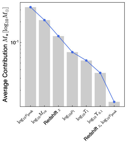
Figure 8: Features with the highest average contribution for the EBM $\gamma(M_{\star}|\bm{\theta})$ trained to predict $M_{\star}$. Average contribution is calculated using the average of the absolute value of the learned functions weighted by the number of samples in each bin (see Equation 5). The features with the largest contributon are $v_{\mathrm{peak}}$ and $M_{\mathrm{vir}}$, followed by redshift $z$, environmental density $\rho_{1}$, environmental temperature $T_{1}$, and mass ratio of nearby halos $\Upsilon_{0.1}$. The interaction with the largest average contribution involves [$z$,$v_{\mathrm{peak}}$].

Average Contributions for the $\gamma(M_{\star}|\bm{\theta})$ EBM
Feature	Value $[\log_{10}M_{\sun}]$
$\beta_{\log_{10}M_{\star}}$	$5.9629$
$\bar{f}(\log_{10}v_{\mathrm{peak}})$	$0.3284$
$\bar{f}(\log_{10}M_{\mathrm{vir}})$	$0.2123$
$\bar{f}(z)$	$0.1238$
$\bar{f}(\log_{10}\rho_{1})$	$0.0722$
$\bar{f}(\log_{10}T_{1})$	$0.0545$
$\bar{f}(\log_{10}\Upsilon_{0.1})$	$0.0359$
$\bar{f}(z,\log_{10}v_{\mathrm{peak}})$	$0.0135$

Table 6: Summary of the EBM model $\gamma(M_{\star}|\bm{\theta})$ trained to predict $M_{\star}$ as a function of the full parameter set $\bm{\theta}$. The first entry, $\beta_{\log_{10}M_{\star}}$, is the learned baseline value of the model (see Section 2.1). The next seven entries are the feature functions with the highest average contribution in descending order. Average contribution is calculated using the average of the absolute value of the feature functions weighted by the number of samples in each bin (see Equation 5).

A.2 Feature Functions

The univariate functions determined by the EBM targeting stellar mass $M_{\star}$ are shown in Figure 9. Stellar mass increases with increasing peak circular velocity, virial mass, environmental density, and neighboring halo mass ratio. Stellar mass increases with decreasing redshift. As with star formation rate, the stellar mass increases with increasing environmental temperature $T_{1}$, with a sharp enhancement near the temperature where hydrogen becomes neutral and a sharp deficit near where hydrogen ionizes.

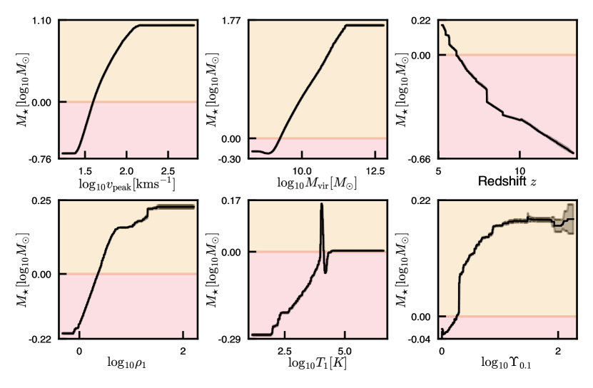
Figure 9: Learned univariate feature functions, $f_{y}^{i}$ in Equation 1, for the EBM $\gamma(M_{\star}|\bm{\theta})$ trained to predict $M_{\star}$. Areas highlighted in orange indicate portions of the function that contribute positively to the predicted $M_{\star}$ and areas in red contribute negatively. Stellar mass increases with peak circular velocity and virial mass, increases with decreasing redshift, and increases with environmental density. Temperature correlates positively with stellar mass, with a strong feature near $T_{1}\approx 10^{4}$ K where hydrogen ionizes. Stellar mass also increases with the mass ratio of neighboring halos.

A.3 Interaction Functions

The bivariate interaction functions $f_{y}^{ij}$ (see Equation 1) learned by the EBM when targeting stellar mass $M_{\star}$ are plotted as heat maps in Figure 10. On average most interaction functions do not contribute significantly to galaxy stellar mass, but there are regions of parameter space where the interaction functions are important. For instance, halos with low environmental temperatures and high environmental densities have suppressed stellar mass. Large virial mass halos with small neighboring halo mass ratios $\log_{10}\Upsilon_{0.1}$, indicating halos that dominate their local environment, have stellar mass enhanced by $\approx 0.3$ dex. This effect exceeds the maximum univariate contribution of $\log_{10}\Upsilon_{0.1}$ alone. The deficit of stellar mass at environmental temperatures where hydrogen is becoming ionized is increased at high redshifts.

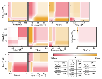
Figure 10: Learned bivariate interaction functions $f_{y}^{ij}$ for the EBM $\gamma(M_{\star}|\bm{\theta})$ trained to predict $M_{\star}$. Areas highlighted in orange indicate portions of the functions that contribute positively to the predicted $M_{\star}$ while areas in red contribute negatively. Halos with large environmental temperatures $T_{1}$ at high redshift $z$ show enhanced stellar mass. The stellar masses of halos with low environmental temperature $T_{1}<10^{4}$K correlate with environmental density, increasing with increasing $\rho_{1}$. Massive halos with no comparable large neighboring halos ($\Upsilon_{0.1}\approx 0$) also show enhanced stellar mass.

Appendix B Composite EBM

The composite EBM (CEBM) models we present consist of a base EBM model trained to recover the main trend $\gamma(y|\bm{\theta}^{\prime})$ of the targeted property $y$ with the input parameters $\bm{\theta}^{\prime}$, an outlier EBM model that captures the outlying values of $y$ not recovered by $\gamma(y|\bm{\theta}^{\prime})$, and a classification EBM model $\phi_{y}(\bm{\theta}^{\prime})$ that interpolates between them (see §4). Given a CEBM, we wish to construct analogs of the average contribution, feature functions, and interaction functions determined for a single EBM. We define these quantities for the CEBM function in §B.2 and B.3 below.

B.1 CEBM Feature and Interaction Functions

The feature functions of a single EBM are univariate and indicate directly how the expectation value of the targeted quantity depends on each parameter $\theta_{i}\in\bm{\theta}$. With a CEBM comprised of a weighted sum of two base EBMs, we define the analog of the feature function to be the weighted sum of the base EBM feature functions. We can write that

$$\tilde{f}^{i}_{y}=\frac{1}{N}\sum_{j=0}^{N}\|\phi(\bm{\theta}_{j})\odot\bm{f}^{i}_{y}(\bm{\theta}_{j})\|_{1},$$ (B1)

where $\odot$ is the Hadamard or element-wise product operation and the sum is over the number of samples $N$. The quantity $\bm{f}^{i}_{y}$ is the vector of the individual EBM feature functions $f_{y}^{i}$. While the base EBM feature functions are individually univariate, by weighting the sum of these feature functions with the classifier EBM the resulting feature function analog in Equation B1 is not univariate.

The interaction functions $\tilde{f}^{ij}_{y}$ are defined as in Equation B1 but with the vector of the individual EBM interaction functions $\bm{f}^{ij}_{y}$ subsituted for $\bm{f}^{i}_{y}$. While the interaction functions for a single EBM are bivariate, the CEBM interaction functions are not bivariate.

B.2 CEBM Average Contribution

The average contribution of each feature in a CEBM can be defined in a manner analogous to the average contribution computed for a single EBM (Equation 5). The CEBM average contribution can be written as

$$\bar{f}_{y}^{i}=\frac{\sum_{j=0}^{n_{b}-1}\tilde{f}(\theta_{i,j})N_{j}}{\sum_{j=0}^{n_{b}-1}N_{j}}$$ (B2)

where $\tilde{f}$ is either the CEBM feature function $\tilde{f}^{i}_{y}$ or the CEBM interaction function $\tilde{f}^{ij}_{y}$. Equation B2 characterizes how important the parameter $\theta_{i}$ is for modeling the target quantity $y$.

B.3 Visualizing CEBM Feature and Interaction Functions

The feature and interaction functions $\tilde{f}^{i}_{y}$ and $\tilde{f}^{ij}_{y}$ are not univariate or bivariate by design, which allows them to model the outlier distribution about the base EBM model $\gamma(y|\bm{\theta}^{\prime})$. To visualize the feature and interaction functions for CEBM models in a manner similar to the univariate feature and bivariate interaction functions for single EBM, we can average the values of $\bm{f}^{i}_{y}$ and $\bm{f}^{ij}_{y}$. For the feature function averaged over $N$ samples, consider $n_{b}$ bins along the $\theta_{i}$ direction, with central values $\theta_{i,b}$ and bin widths $\Delta\theta_{i,b}$. The bin-averaged CEBM feature and interaction functions are then

$$f^{i,b}_{y}=\frac{1}{N}\sum_{j=0}^{N-1}\alpha(\theta_{i,b},\Delta\theta_{i,b},\theta_{j,i})\phi(\bm{\theta}_{j})\odot\bm{f}(\bm{\theta}_{j})$$ (B3)

where $\theta_{j,i}$ is the $i$th parameter of the $j$th sample $\bm{\theta}_{j}$ and the function $\alpha(\theta_{i,b},\Delta\theta_{i,b},\theta_{j,i})=1$ if $\theta_{i,b}-\Delta\theta_{i,b}/2\leq\theta_{j,i}\leq\theta_{i,b}+\Delta\theta_{i,b}/2$ and $\alpha=0$ otherwise. The quantity $\bm{f}$ is either the vector of EBM feature functions $\bm{f}^{i}_{y}$ or the EBM interaction functions $\bm{f}^{ij}_{y}$. Equation B3 calculates the mean of the $\bm{f}$ values in each of the $n_{b}$ bins, and can be modified to calculate its standard deviation.

Appendix C Composite EBM Model for Star Formation Rate

The CEBM model $\Gamma(S\!F\!R|\bm{\theta}^{\prime})$ for the star formation rate consists of a base EBM $\gamma(S\!F\!R|\bm{\theta}^{\prime})$, a residual EBM $\delta(S\!F\!R|\bm{\theta}^{\prime})$ that attempts to capture the outlying values of $S\!F\!R$ not recovered by $\gamma(S\!F\!R|\bm{\theta}^{\prime})$, and the classifier EBM $\phi_{S\!F\!R}(\bm{\theta}^{\prime})$. For each of these individual EBMs that form the CEBM model, we plot the average contribution, feature functions, and interaction functions.

Figure 11 shows the average contribution, feature functions, and interaction functions for the EBM model $\gamma(S\!F\!R|\bm{\theta}^{\prime})$ that forms the base of the CEBM model. The differences between $\gamma(S\!F\!R|\bm{\theta})$ and $\gamma(S\!F\!R|\bm{\theta}^{\prime})$ reflect the additional information provided by the maximum peak circular velocity $v_{\mathrm{peak}}$. Without access to $v_{\mathrm{peak}}$, the base EBM $\gamma(S\!F\!R|\bm{\theta}^{\prime})$ upweights $\bar{f}(M_{\mathrm{vir}})$ such that its importance roughly equals the combined importance of $M_{\mathrm{vir}}$ and $v_{\mathrm{peak}}$ in determining $\gamma(S\!F\!R|\bm{\theta})$. The average contribution of $\rho_{1}$, $T_{1}$, $z$, $\Upsilon_{0.1}$, and $(M_{\mathrm{vir}},\Upsilon_{0.1})$ are similar between the models. The additional interaction term in the top seven average contributions is $(z,\rho_{1})$, with a percent-level contribution to $S\!F\!R$ relative to $M_{\mathrm{vir}}$. The feature functions for $\gamma(S\!F\!R|\bm{\theta}^{\prime})$ have shapes similar to the feature functions for $\gamma(S\!F\!R|\bm{\theta})$, but their minimum and maximum contributions to $S\!F\!R$ are adjusted to account for the missing $v_{\mathrm{peak}}$ contribution. The feature function $\bar{f}(z)$ is noisier overall. For the interaction functions, the largest contributors now involve $M_{\mathrm{vir}}$ rather than the missing parameter $v_{\mathrm{peak}}$, and the set of available functions is substantially different than with $\gamma(S\!F\!R|\bm{\theta})$.

Figure 12 shows the average contribution, feature functions, and interaction functions for the outlier EBM $\delta(S\!F\!R|\bm{\theta}^{\prime})$ fit to the deviant samples not captured by the base EBM $\gamma(S\!F\!R|\bm{\theta}^{\prime})$. The outlier EBM receives the highest contribution from virial mass, with an average contribution more than an order of magnitude larger than the next most important feature $\rho_{1}$. The redshift $z$ and environmental temperature $T_{1}$ have comparable importance to $\rho_{1}$. The remaining features provide only percent-level contributions relative to $M_{\mathrm{vir}}$.

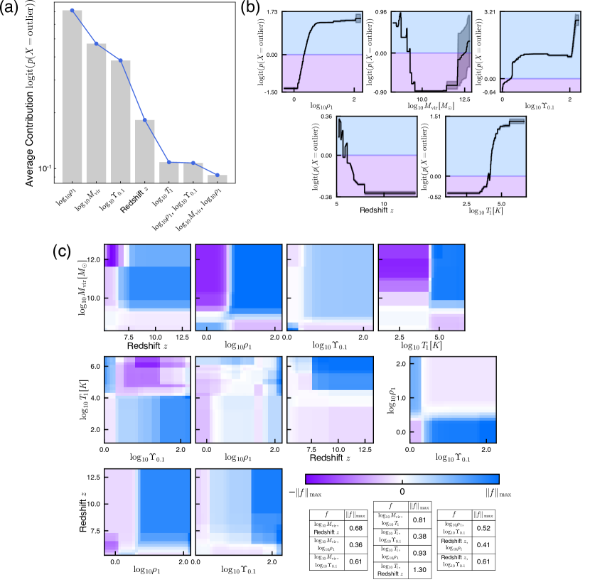
Figure 13: Details for the classification EBM model $\phi_{S\!F\!R}(\bm{\theta}^{\prime})$ that interpolates between the base EBM $\gamma(S\!F\!R|\bm{\theta}^{\prime})$ and the outlier EBM $\delta(S\!F\!R|\bm{\theta}^{\prime})$ for creating the CEBM $\Gamma(S\!F\!R|\bm{\theta}^{\prime})$. Panel a) displays the average contribution of features to the classification EBM model $\phi_{S\!F\!R}(\bm{\theta}^{\prime})$. The most important features for determining whether a galaxy is an outlier in the SFR distribution are environmental density $\rho_{1}$, virial mass $M_{\mathrm{vir}}$, and nearby halo mass ratio $\Upsilon_{0.1}$. The average contributions are unit free, and represent changes to the log odds of a galaxy being an outlier in the SFR distribution. Panel b) shows the feature functions contributing to the classifier EBM $\phi_{S\!F\!R}(\bm{\theta}^{\prime})$. These feature functions represent the change in log odds that a given galaxy will be an outlier in SFR. Outliers tend to occur at high environmental density $\rho_{1}$ or very low or high virial masses $M_{\mathrm{vir}}$. Galaxies with massive neighbors, reflected by $\Upsilon_{0.1}$, or high environmental temperature $T_{1}$ are also more likely to be outliers. The lowest redshift galaxies in the dataset are additionally likely be outliers in SFR. Panel c) presents the interaction functions for the classifier EBM $\phi_{S\!F\!R}(\bm{\theta}^{\prime})$. Each panel shows the contributions of the interaction terms, normalized such that the color map ranges between plus or minus the maximum of the norm of each function $||f||_{\mathrm{max}}$. Purple indicates negative log odds and blue indicates positive log odds that a given galaxy is an outlier in SFR. The table lists $||f||_{\mathrm{max}}$ for the interaction functions, listed as the corresponding change in log odds. Galaxies with large environmental temperature $T_{1}$ and with high environmental density $\rho_{1}$, at high redshift $z$, or with large virial mass $M_{\mathrm{vir}}$ are more likely to be outliers. Massive galaxies in high environmental densities or at high redshift also are more likely outliers in SFR.

Figure 13 shows the average contribution, feature functions, and interaction functions for the classifier EBM $\delta(S\!F\!R|\bm{\theta}^{\prime})$ that interpolates between the base and outlier EBMs when calculating the CEBM model. For the classifier EBM, the most important features are $\rho_{1}$, $M_{\mathrm{vir}}$, and $\Upsilon_{0.1}$. Redshift $z$ has middling importance, following by $T_{1}$, $[\rho_{1},\Upsilon_{0.1}]$, and $[M_{\mathrm{vir}},\rho_{1}]$. The feature functions show strong dependencies on $\rho_{1}$, $M_{\mathrm{vir}}$, $\Upsilon_{0.1}$, $z$, and $T_{1}$. The largest interaction functions involve the environmental temperature $T_{1}$, redshift $z$, and virial mass $M_{\mathrm{vir}}$.

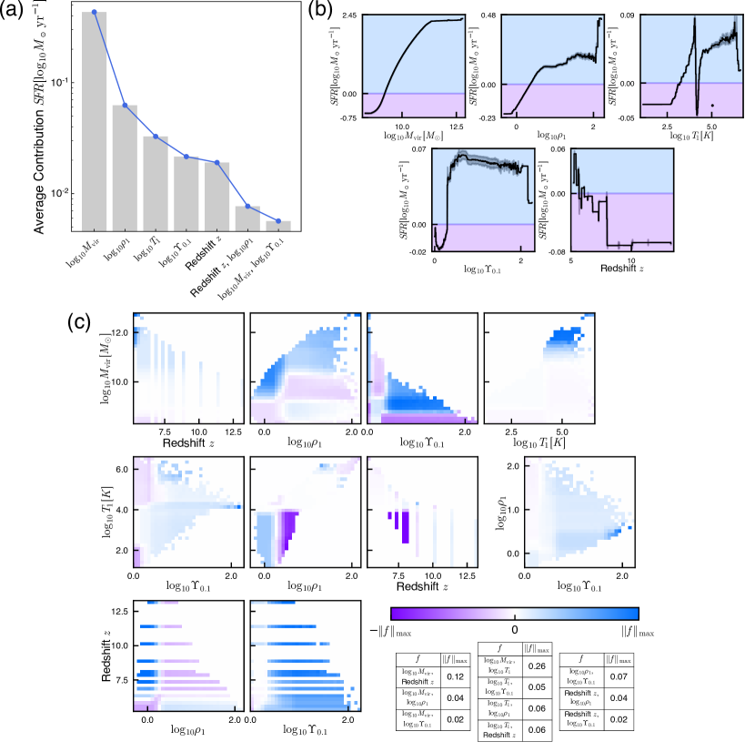
Figure 14: Details for the CEBM model $\Gamma(S\!F\!R|\bm{\theta}^{\prime})$ trained to predict $S\!F\!R$. Panel a) displays the average contribution of features to the CEBM. Virial mass $M_{\mathrm{vir}}$ provides the largest average contribution to the star formation rate. The environmental density $\rho_{1}$ provides a $\sim 6\times$ smaller average contribution. The environmental temperature $T_{1}$, nearby galaxy mass ratio $\Upsilon_{0.1}$, and redshift $z$ provide a relative contribution roughly $10\times$ smaller than $M_{\mathrm{vir}}$. Panel b) shows the feature functions contributing to the CEBM $\Gamma(S\!F\!R|\bm{\theta}^{\prime})$. The SFR increases with $M_{\mathrm{vir}}$, which provides the largest contribution. A secondary contribution comes from environmental density $\rho_{1}$. Environmental temperature $T_{1}$ has a minor contribution, but shows the familiar feature at $T_{1}\approx 10^{4}$K where hydrogen ionizes. The mass ratio of nearby halos $\Upsilon_{0.1}$ and redshift $z$ provide minor contributions. As expected, the CEBM feature functions are similar to the base EBM feature functions that represent the parameter dependence of star formation rate for most galaxies in the dataset (see Panel b) of Figure 11). Panel c) presents the interaction functions for the CEBM $\Gamma(S\!F\!R|\bm{\theta}^{\prime})$. Each panel shows the contribution of the interaction terms, normalized such that the color map ranges between plus or minus the maximum of the norm of each function $||f||_{\mathrm{max}}$. Purple indicates negative contributions and blue indicates positive contributions. The table lists $||f||_{\mathrm{max}}$ for the interaction functions, each with units $\log_{10}M_{\sun}~{}\mathrm{yr}^{-1}$. As for the interaction functions for the base EBM $\gamma(S\!F\!R|\bm{\theta}^{\prime})$, the largest interaction occurs for large virial mass $M_{\mathrm{vir}}$ and large environmental temperature $T_{1}$ or low redshift $z$.

By weighting the base and outlier EBM models with the classifier EBM, we construct the CEBM for star formation rate as $\Gamma(S\!F\!R|\bm{\theta}^{\prime})\equiv[1-\phi_{S\!F\!R}(\bm{\theta}^{\prime})]\gamma(S\!F\!R|\bm{\theta}^{\prime})+\phi_{S\!F\!R}(\bm{\theta}^{\prime})\delta(S\!F\!R|\bm{\theta}^{\prime})$. Figures 14 show the average contribution, feature functions, and interaction functions for the $S\!F\!R$ CEBM. The most important feature is $M_{\mathrm{vir}}$, which dominates by a factor of $\sim 4-10$ over environmental density $\rho_{1}$, environmental temperature $T_{1}$, $\Upsilon_{0.1}$, and redshift $z$. The interaction terms are roughly percent-level effects relative to $M_{\mathrm{vir}}$. The feature functions show a strongly increasing $S\!F\!R$ with $M_{\mathrm{vir}}$, and enhanced $S\!F\!R$ with environmental density $\rho_{1}$. The temperature dependence shows the feature at $\log_{10}T_{1}\approx 4$ seen with the EBM model $\gamma(S\!F\!R|\bm{\theta})$. The interaction functions provide only important contributions over very limited areas of parameter space, with the most important adjustments occuring at low redshift and large virial mass, or for large temperatures and virial masses. For reference, the model summary Figure 6 illustrates the overall performance of the model.

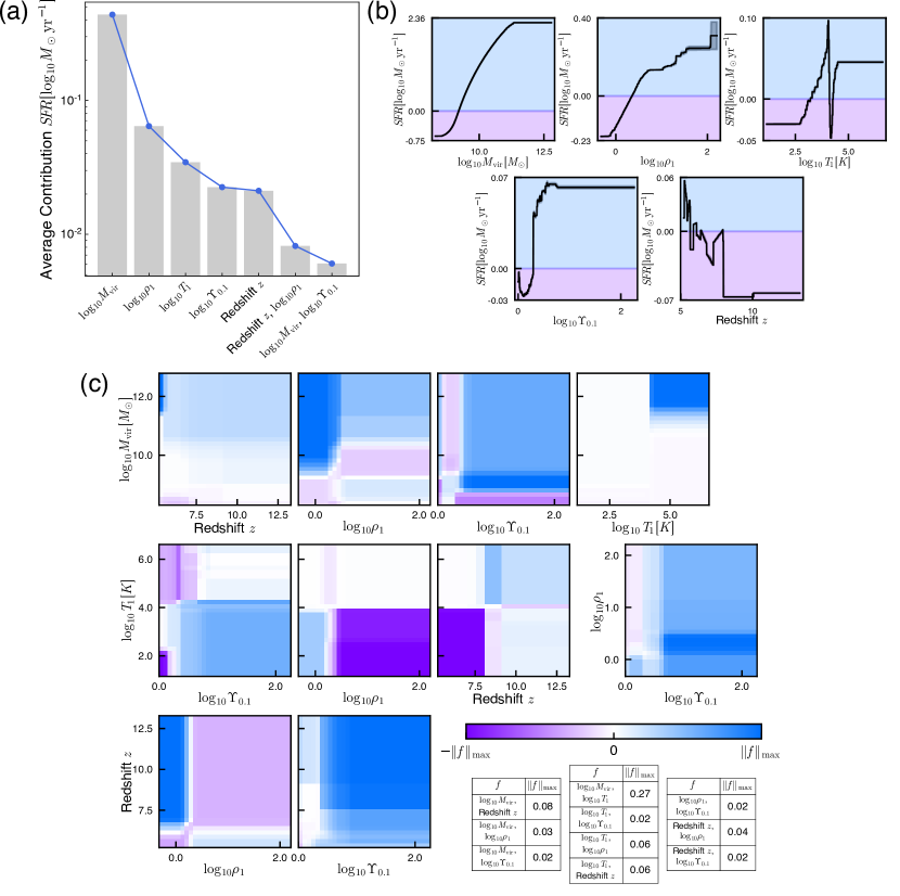
Figure 11: Details for the base EBM model $\gamma(S\!F\!R|\bm{\theta}^{\prime})$ component of the CEBM $\Gamma(S\!F\!R|\bm{\theta}^{\prime})$ trained to predict $S\!F\!R$. Panel a) displays the average contribution of features. The dominant feature is virial mass $M_{\mathrm{vir}}$, with an average contribution to $\log_{10}S\!F\!R$ roughly $8-10\times$ larger than environmental density $\rho_{1}$ and temperature $T_{1}$. Compared with the average contributions to the EBM $\gamma(S\!F\!R|\bm{\theta})$ (see Figure 1), $M_{\mathrm{vir}}$ subsumes the contribution provided by the missing $v_{\mathrm{peak}}$ parameter. Panel b) shows the feature functions contributing to the base EBM model. The SFR increases with $M_{\mathrm{vir}}$, which provides the dominant contribution. A secondary contribution comes from environmental density $\rho_{1}$. Environmental temperature $T_{1}$ has a minor contribution, but shows the same feature at $T_{1}\approx 10^{4}$K where hydrogen ionizes. The mass ratio of nearby halos $\Upsilon_{0.1}$ and redshift $z$ provide minor contributions. Panel c) presents the interaction functions for the base EBM $\gamma(S\!F\!R|\bm{\theta}^{\prime})$. Each panel shows the contribution of the bivariate interaction terms, normalized such that the color map ranges between plus or minus the maximum of the norm of each function $||f||_{\mathrm{max}}$. Purple indicates negative contributions and blue indicates positive contributions. The table lists $||f||_{\mathrm{max}}$ for the interaction functions, each with units $\log_{10}M_{\sun}~{}\mathrm{yr}^{-1}$. In absolute terms, the largest interaction occurs for large virial mass $M_{\mathrm{vir}}$ and environmental temperature $T_{1}$. SFR is partially reduced for low environmental temperature $T_{1}$ and either low environmental density $\rho_{1}$ or redshift $z$.

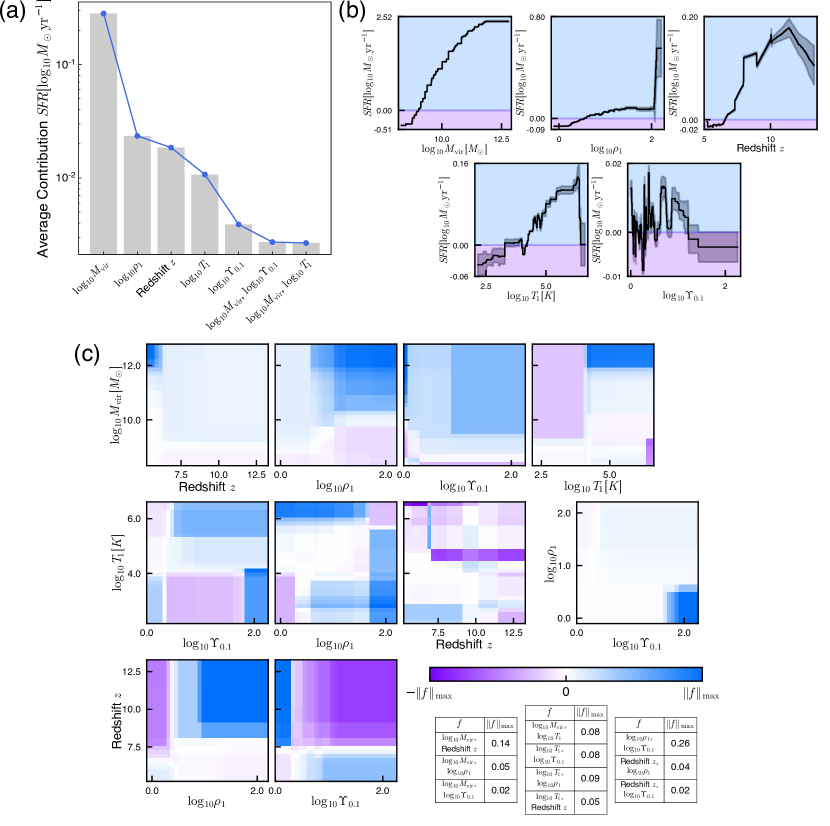
Figure 12: Details for the outlier EBM model $\delta(S\!F\!R|\bm{\theta}^{\prime})$ component of the CEBM $\Gamma(S\!F\!R|\bm{\theta}^{\prime})$ trained to predict $S\!F\!R$. Panel a) displays the average contribution of features. As with the base EBM $\gamma(S\!F\!R|\bm{\theta}^{\prime})$, the feature with the largest average contribution is virial mass $M_{\mathrm{vir}}$, with roughly $\gtrsim 10\times$ larger contribution to $\log_{10}S\!F\!R$ than environmental density $\rho_{1}$, redshift $z$, or temperature $T_{1}$. The average contributions of $\Upsilon_{0.1}$ or interactions are small. Panel b) shows the feature functions for the outlier EBM $\delta(S\!F\!R|\bm{\theta}^{\prime})$. The feature function for virial mass $M_{\mathrm{vir}}$ has the largest contribution to $\delta(S\!F\!R|\bm{\theta}^{\prime})$, similar to the virial mass dependence of the base EBM $\gamma(S\!F\!R|\bm{\theta}^{\prime})$ (see Panel b) of Figure 11). The SFR of outliers increases with increasing environmental density $\rho_{1}$, with a large enhancement at very large $\rho_{1}$. Unlike the base EBM $\gamma(S\!F\!R|\bm{\theta}^{\prime})$, SFR for the outliers increases with increasing redshift. The feature function for the nearby halo mass ratio $\Upsilon_{0.1}$ is weak and noisy. Panel c) presents the interaction functions for the outlier EBM $\delta(S\!F\!R|\bm{\theta}^{\prime})$. Each panel shows the contribution of the bivariate interaction terms, normalized such that the color map ranges between plus or minus the maximum of the norm of each function $||f||_{\mathrm{max}}$. Purple indicates negative contributions and blue indicates positive contributions. The table lists $||f||_{\mathrm{max}}$ for the interaction functions, each with units $\log_{10}M_{\sun}~{}\mathrm{yr}^{-1}$. For outliers, the SFR increases at low environmental density $\rho_{1}$ and large neighboring halo mass ratios $\Upsilon_{0.1}$, suggesting dynamical interactions increase star formation rate in low density environments. The other interaction functions are relatively weak.

Appendix D Composite EBM Model for Stellar Mass

The CEBM model $\Gamma(M_{\star}|\bm{\theta}^{\prime})$ for stellar mass is comprised of a base EBM $\gamma(M_{\star}|\bm{\theta}^{\prime})$, an outlier EBM that attempts to model the $M_{\star}$ of samples not recovered by $\gamma(M_{\star}|\bm{\theta}^{\prime})$, and the classifier EBM function $\phi_{M_{\star}}(\bm{\theta}^{\prime})$ that interpolates between them. The average contribution, feature functions, and interaction functions from these component EBM models are presented below.

Figures 15 shows the average contribution, feature functions, and interaction functions for the base EBM model $\gamma(M_{\star}|\bm{\theta}^{\prime})$. By removing $v_{\mathrm{peak}}$ from the dataset used to train the EBM, the base EBM model for the $M_{\star}$ CEBM replaces the dependence on $v_{\mathrm{peak}}$ with an additional dependence on $M_{\mathrm{vir}}$. The relative ordering and importance of redshift $z$, environmental density $\rho_{1}$, environmental temperature $T_{1}$, and $\Upsilon_{0.1}$ are approximately maintained. For the feature functions, the results shown for $\gamma(M_{\star}|\bm{\theta}^{\prime})$ in Panel b) of Figure 15 can be compared with the results for $\gamma(M_{\star}|\bm{\theta})$ shown in Figure 8. As reflected by average contributions, the amplitude of the feature function $\bar{f}(M_{\mathrm{vir}})$ increases to account for the removal of $v_{\mathrm{peak}}$. The feature functions for $z$, $\rho_{1}$, $T_{1}$, and $\Upsilon_{0.1}$ are modified and remain similar in shape to those computed for the EBM $\gamma(M_{\star}|\bm{\theta})$. The interaction functions shared between $\gamma(M_{\star}|\bm{\theta}^{\prime})$ and $\gamma(M_{\star}|\bm{\theta})$ are similar. There is an increase in $M_{\star}$ contribution for large $[M_{\mathrm{vir}},T_{1}]$ and a decrease in the amplitude of $[M_{\mathrm{vir}},\Upsilon_{0.1}]$.

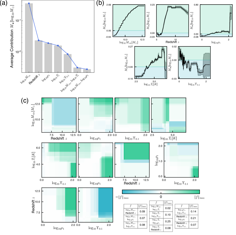
Figure 16: Details for the outlier EBM model $\delta(M_{\star}|\bm{\theta}^{\prime})$ component of the CEBM $\Gamma(M_{\star}|\bm{\theta}^{\prime})$ trained to predict $M_{\star}$. Panel a) displays the average contribution of features to the outlier EBM model $\delta(M_{\star}|\bm{\theta}^{\prime})$. As with the base EBM $\gamma(M_{\star}|\bm{\theta}^{\prime})$, the feature with the largest average contribution is virial mass $M_{\mathrm{vir}}$, with roughly $\gtrsim 10\times$ larger contribution to $\log_{10}M_{\star}$ than redshift $z$, environmental density $\rho_{1}$, or temperature $T_{1}$. The average contributions of $\Upsilon_{0.1}$ or interactions are small. Panel b) shows the feature functions for the outlier EBM $\delta(M_{\star}|\bm{\theta}^{\prime})$. The feature function for virial mass $M_{\mathrm{vir}}$ has the largest contribution to $\delta(S\!F\!R|\bm{\theta}^{\prime})$, similar to the virial mass dependence of the base EBM $\gamma(M_{\star}|\bm{\theta}^{\prime})$ (see Panel b) of Figure 15). The stellar mass of outliers increases with increasing environmental density $\rho_{1}$, with a large enhancement at very large $\rho_{1}$. Unlike the base EBM $\gamma(M_{\star}|\bm{\theta}^{\prime})$, the stellar mass of the outliers increases with increasing redshift. The feature function for the nearby halo mass ratio $\Upsilon_{0.1}$ is weak and noisy. Panel c) presents the interaction functions for the outlier EBM $\delta(M_{\star}|\bm{\theta}^{\prime})$. Each panel shows the contribution of the interaction terms, normalized such that the color map ranges between plus or minus the maximum of the norm of each function $||f||_{\mathrm{max}}$. Teal indicates negative contributions and green indicates positive contributions. The table lists $||f||_{\mathrm{max}}$ for the interaction functions, each with units $\log_{10}M_{\sun}$. For outliers, stellar mass increases at high environmental density $\rho_{1}$ with low environmental temperature $T_{1}$ or high redshift $z$.

Figure 16 shows the average contribution, feature functions, and interaction functions for the outlier EBM model $\delta(M_{\star}|\bm{\theta}^{\prime})$. The average contribution is dominated by $M_{\mathrm{vir}}$, with the contributions from all other single parameters lower by a factor of $\approx 10$ with the order of importance maintained relative to $\gamma(M_{\star}|\bm{\theta}^{\prime})$. For the feature functions, the redshift dependence changes dramatically and now increases with increasing redshift. The feature function for environmental density $\tilde{f}(\rho_{1})$ becomes much weaker over a wide range of $\rho_{1}$, but increases dramatically at high $\rho_{1}$. Relative to the $\gamma(M_{\star}|\bm{\theta}^{\prime})$ feature functions, the feature function $\tilde{f}(\Upsilon_{0.1})$ for $\delta(M_{\star}|\bm{\theta}^{\prime})$ is weak and noisy. The interaction functions show increased contributions at large $[z,\rho_{1}]$, and for low $T_{1}$ and large $\rho_{1}$.

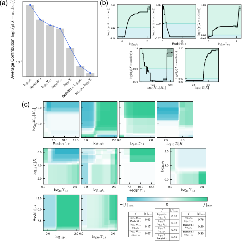
Figure 17: Details for the classification EBM model $\phi_{M_{\star}}(\bm{\theta}^{\prime})$ that interpolates between the base EBM $\gamma(M_{\star}|\bm{\theta}^{\prime})$ and the outlier EBM $\delta(M_{\star}|\bm{\theta}^{\prime})$ for creating the CEBM $\Gamma(M_{\star}|\bm{\theta}^{\prime})$. Panel a) displays the average contribution of features to the classification EBM model $\phi_{M_{\star}}(\bm{\theta}^{\prime})$. The most important features for determining whether a galaxy is an outlier in the stellar mass distribution are environmental density $\rho_{1}$, redshift $z$, nearby halo mass ratio $\Upsilon_{0.1}$, and virial mass $M_{\mathrm{vir}}$. The average contributions are unit free, and represent changes to the log odds of a galaxy being an outlier in the stellar mass distribution. Panel b) shows the feature functions contributing to the classifier EBM $\phi_{M_{\star}}(\bm{\theta}^{\prime})$. These feature functions represent the change in log odds that a given galaxy will be an outlier in $M_{\star}$. Outliers tend to occur at high environmental density $\rho_{1}$ or very low or high virial masses $M_{\mathrm{vir}}$. Galaxies with massive neighbors, reflected by $\Upsilon_{0.1}$, or high environmental temperature $T_{1}$ are also more likely to be outliers. The lowest redshift galaxies in the dataset are additionally likely be outliers in stellar mass. These trends are similar to the feature functions for the classifier EBM $\phi_{S\!F\!R}(\bm{\theta}^{\prime})$ (see Panel b) of Figure 13). Panel c) presents the interaction functions for the classifier EBM $\phi_{M_{\star}}(\bm{\theta}^{\prime})$. Each panel shows the contributions of the interaction terms, normalized such that the color map ranges between plus or minus the maximum of the norm of each function $||f||_{\mathrm{max}}$. Teal indicates negative log odds and green indicates positive log odds that a given galaxy is an outlier in stellar mass. The table lists $||f||_{\mathrm{max}}$ for the interaction functions, listed as the corresponding change in log odds. Galaxies with large environmental temperature $T_{1}$ and at high redshift $z$ are more likely to be outliers. Massive galaxies at high environmental density $\rho_{1}$ or with large nearby halos (large $\Upsilon_{0.1}$) also tend to be outliers. Galaxies at low environmental density but with large nearby halos are also have an increased likelihood of being outliers in stellar mass.

Figure 17 shows the average contribution, feature functions, and interaction functions for the classifier EBM $\phi_{M_{\star}}(\bm{\theta}^{\prime})$. For each of these properties, we note that in determining $\phi_{M_{\star}}(\bm{\theta}^{\prime})$ a sigmoid function $\sigma$ is applied to the sum of $\beta$, $f_{y}^{i}$ and $f_{y}^{ij}$ that model the log odds that a galaxy is an outlier in stellar mass. In determining $M_{\star}$, the features with the largest average contribution are environmental density $\rho_{1}$, redshift $z$, $\Upsilon_{0.1}$, and virial mass $M_{\mathrm{vir}}$. The interaction terms with the largest contribution are $(z,\rho_{1})$ and $(\rho_{1},T_{1})$. Clearly, environmental density plays an important role in determining whether a given simulated galaxy is an outlier relative to the base EBM $\gamma(M_{\star}|\bm{\theta}^{\prime})$. The feature functions show that galaxies with large environmental densities $\rho_{1}$, at low redshift $z$, or with a large neighboring galaxy (expressed by $\Upsilon_{0.1}$) have an enhanced probability of being outliers relative to $\gamma(M_{\star}|\bm{\theta}^{\prime})$. Galaxies at both high and low $M_{\mathrm{vir}}$ or large environmental temperature $T_{1}$ are also more likely to be outliers.

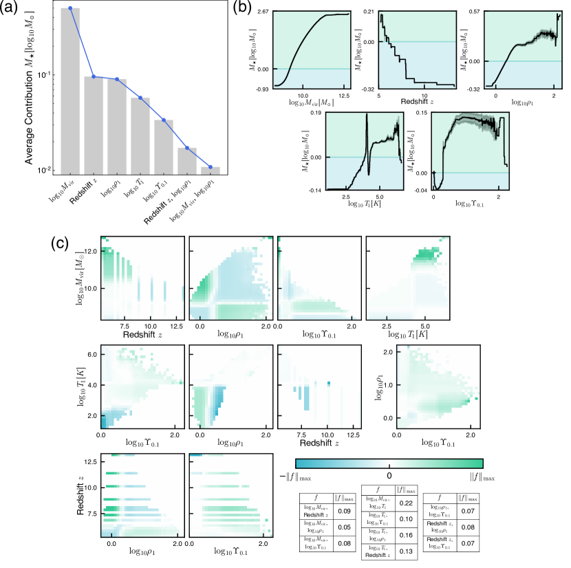
Figure 18: Details for the CEBM model $\Gamma(M_{\star}|\bm{\theta}^{\prime})$ trained to predict stellar mass $M_{\star}$. Panel a) displays the average contribution of features to the CEBM model $\Gamma(M_{\star}|\bm{\theta}^{\prime})$. Virial mass $M_{\mathrm{vir}}$ provides the largest average contribution to the stellar mass. The environmental density $\rho_{1}$ and redshift $z$ provide $\sim 5\times$ smaller average contributions. The environmental temperature $T_{1}$ and nearby galaxy mass ratio $\Upsilon_{0.1}$ provide a relative contribution to stellar mass roughly $10\times$ smaller than $M_{\mathrm{vir}}$. Panel b) shows the feature functions contributing to the CEBM $\Gamma(M_{\star}|\bm{\theta}^{\prime})$. The stellar mass increases with $M_{\mathrm{vir}}$, which provides the largest contribution. Secondary contributions come from environmental density $\rho_{1}$ and redshift $z$. Environmental temperature $T_{1}$ has a smaller contribution, but shows the familiar feature at $T_{1}\approx 10^{4}$K where hydrogen ionizes. The mass ratio of nearby halos $\Upsilon_{0.1}$ provides a minor contribution. As expected, the CEBM feature functions resemble the base EBM feature functions that represent the parameter dependence of stellar mass for most galaxies in the dataset (see Panel b) of Figure 15). Panel c) presents the interaction functions for the CEBM $\Gamma(M_{\star}|\bm{\theta}^{\prime})$. Each panel shows the contribution of the interaction terms, normalized such that the color map ranges between plus or minus the maximum of the norm of each function $||f||_{\mathrm{max}}$. Teal indicates negative contributions and green indicates positive contributions. The table lists $||f||_{\mathrm{max}}$ for the interaction functions, each with units $\log_{10}M_{\sun}$. As for the interaction functions for the base EBM $\gamma(M_{\star}|\bm{\theta}^{\prime})$, the largest interaction occurs for large virial mass $M_{\mathrm{vir}}$ and large environmental temperature $T_{1}$. Stellar mass is partially reduced for low environmental temperature $T_{1}$ and high environmental density $\rho_{1}$. These trends are similar to those for the base EBM $\gamma(M_{\star}|\bm{\theta}^{\prime})$ modeling stellar mass (see Panel c) of Figure 15).

We construct the stellar mass CEBM with the sum $\Gamma(M_{\star}|\bm{\theta}^{\prime})\equiv[1-\phi_{M_{\star}}(\bm{\theta}^{\prime})]\gamma(M_{\star}|\bm{\theta}^{\prime})+\phi_{M_{\star}}(\bm{\theta}^{\prime})\delta(M_{\star}|\bm{\theta}^{\prime})$. Figure 18 shows the average contribution, feature functions, and interaction functions for $\Gamma(M_{\star}|\bm{\theta}^{\prime})$. The feature with largest average contribution is $M_{\mathrm{vir}}$, with redshift $z$, environmental density $\rho_{1}$, environmental temperature $T_{1}$, and the mass ratio of nearby galaxies $\Upsilon_{0.1}$ having an lower average contribution by a factor of $\sim 5-10$. Relative to $M_{\mathrm{vir}}$, the interactions $[z,\rho_{1}]$ and $[M_{\mathrm{vir}},\rho_{1}]$ contribute at level of a few percent. The $M_{\star}$ CEBM feature function $\tilde{f}(M_{\mathrm{vir}})$ has increased in amplitude relative to the $M_{\star}$ EBM feature function $f(M_{\mathrm{vir}})$, subsuming some of the dependence on the missing $v_{\mathrm{peak}}$ feature. The remaining feature functions for $\Gamma(M_{\star}|\bm{\theta}^{\prime})$ are similar in shape and amplitude to those for $\gamma(M_{\star}|\bm{\theta})$, although the contribution at large $T_{1}$ and $\rho_{1}$ are increased and the dependence on redshift $z$ is decreased. The interaction functions are similar between $\Gamma(M_{\star}|\bm{\theta}^{\prime})$ and $\gamma(M_{\star}|\bm{\theta}^{\prime})$, although there is a larger enhancement of $M_{\star}$ for large $[M_{\mathrm{vir}},T_{1}]$ and a smaller enhancement for large $M_{\mathrm{vir}}$ and small $\Upsilon_{0.1}$ for the CEBM $\Gamma(M_{\star}|\bm{\theta}^{\prime})$. For reference, the model summary Figure 7 illustrates the overall performance of the model.

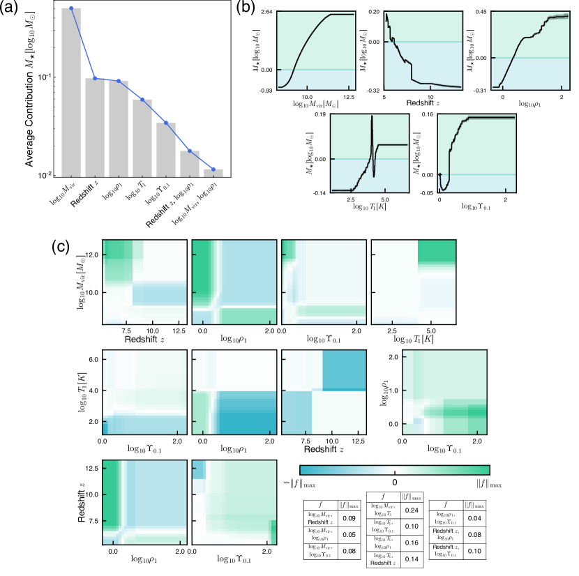
Figure 15: Details for the base EBM model $\gamma(M_{\star}|\bm{\theta}^{\prime})$ component of the CEBM $\Gamma(M_{\star}|\bm{\theta}^{\prime})$ trained to predict stellar mass $M_{\star}$. Panel a) displays the average contribution of features to the base EBM model $\gamma(M_{\star}|\bm{\theta}^{\prime})$. The feature with the highest average contribution is virial mass $M_{\mathrm{vir}}$, with an average contribution to $\log_{10}M_{\star}$ roughly $5\times$ larger than that from redshift $z$ or environmental density $\rho_{1}$. The environmental temperature $T_{1}$ and nearby halo mass ratio $\Upsilon_{0.1}$ provide smaller average contributions, and interactions between features are yet smaller. Panel b) shows the feature functions contributing to the base EBM model $\gamma(M_{\star}|\bm{\theta}^{\prime})$. The stellar mass increases with $M_{\mathrm{vir}}$ that provides the largest contribution. Secondary contributions come from redshift $z$, which increases $M_{\star}$ at later times, and the positive correlate environmental density $\rho_{1}$. comes from environmental density $\rho_{1}$. Environmental temperature $T_{1}$ has a small contribution, and shows the familiar feature at $T_{1}\approx 10^{4}$K where hydrogen ionizes. The mass ratio of nearby halos $\Upsilon_{0.1}$ provides a minor contribution. Panel c) presents the interaction functions for the base EBM $\gamma(M_{\star}|\bm{\theta}^{\prime})$. Each panel shows the contribution of the bivariate interaction terms, normalized such that the color map ranges between plus or minus the maximum of the norm of each function $||f||_{\mathrm{max}}$. Teal indicates negative contributions and green indicates positive contributions. The table lists $||f||_{\mathrm{max}}$ for the interaction functions, each with units $\log_{10}M_{\sun}$. In absolute terms, the largest interaction occurs for large virial mass $M_{\mathrm{vir}}$ and environmental temperature $T_{1}$ (same as for the base EBM $\gamma(S\!F\!R|\bm{\theta}^{\prime})$ modeling star formation rate, see Panel c) of Figure 11). Stellar mass is partially reduced for low environmental temperature $T_{1}$ and either high environmental density $\rho_{1}$ or high redshift $z$.

Average Contributions for the CEBM $\Gamma(M_{\star}|\bm{\theta}^{\prime})$
Feature	Value $[\log_{10}M_{\sun}]$
$\beta_{\log_{10}M_{\star}}$	$6.6995$
$\tilde{f}(\log_{10}M_{\mathrm{vir}})$	$0.5008$
$\tilde{f}(z)$	$0.0961$
$\tilde{f}(\log_{10}\rho_{1})$	$0.0902$
$\tilde{f}(\log_{10}T_{1})$	$0.0576$
$\tilde{f}(\log_{10}\Upsilon_{0.1})$	$0.0336$
$\tilde{f}(z,\log_{10}\rho_{1})$	$0.0172$
$\tilde{f}(\log_{10}M_{\mathrm{vir}},\log_{10}\rho_{1})$	$0.0108$

Table 7: Summary of the CEBM model $\Gamma(M_{\star}|\bm{\theta}^{\prime})$ trained to predict $M_{\star}$ using the restricted parameter set $\bm{\theta}^{\prime}$. The first entry, $\beta_{\log_{10}M_{\star}}$, is the learned baseline of the model. The next seven entries are the learned functions with the highest average contribution in descending order. The average contribution is computed via Equation B2 (see §B.2 for more details).

References

- Balogh et al. (2004) Balogh, M. L., Baldry, I. K., Nichol, R., et al. 2004, ApJ, 615, L101, doi: 10.1086/426079
- Behroozi et al. (2019) Behroozi, P., Wechsler, R. H., Hearin, A. P., & Conroy, C. 2019, MNRAS, 488, 3143, doi: 10.1093/mnras/stz1182
- Bluck et al. (2022) Bluck, A. F. L., Maiolino, R., Brownson, S., et al. 2022, A&A, 659, A160, doi: 10.1051/0004-6361/202142643
- Bouwens et al. (2012) Bouwens, R. J., Illingworth, G. D., Oesch, P. A., et al. 2012, ApJ, 754, 83, doi: 10.1088/0004-637X/754/2/83
- Brinchmann et al. (2004) Brinchmann, J., Charlot, S., White, S. D. M., et al. 2004, MNRAS, 351, 1151, doi: 10.1111/j.1365-2966.2004.07881.x
- Conroy et al. (2006) Conroy, C., Wechsler, R. H., & Kravtsov, A. V. 2006, ApJ, 647, 201, doi: 10.1086/503602
- Contini et al. (2020) Contini, E., Gu, Q., Ge, X., et al. 2020, ApJ, 889, 156, doi: 10.3847/1538-4357/ab6730
- Croton et al. (2016) Croton, D. J., Stevens, A. R. H., Tonini, C., et al. 2016, ApJS, 222, 22, doi: 10.3847/0067-0049/222/2/22
- Davé et al. (2019) Davé, R., Anglés-Alcázar, D., Narayanan, D., et al. 2019, MNRAS, 486, 2827, doi: 10.1093/mnras/stz937
- Davies et al. (2016) Davies, L. J. M., Robotham, A. S. G., Driver, S. P., et al. 2016, MNRAS, 455, 4013, doi: 10.1093/mnras/stv2573
- Davies et al. (2019) Davies, L. J. M., Robotham, A. S. G., Lagos, C. d. P., et al. 2019, MNRAS, 483, 5444, doi: 10.1093/mnras/sty3393
- Faber et al. (2007) Faber, S. M., Willmer, C. N. A., Wolf, C., et al. 2007, ApJ, 665, 265, doi: 10.1086/519294
- Friedman (2001) Friedman, J. H. 2001, The Annals of Statistics, 29, 1189 , doi: 10.1214/aos/1013203451
- Girelli et al. (2020) Girelli, G., Pozzetti, L., Bolzonella, M., et al. 2020, A&A, 634, A135, doi: 10.1051/0004-6361/201936329
- Gnedin (2014) Gnedin, N. Y. 2014, ApJ, 793, 29, doi: 10.1088/0004-637X/793/1/29
- Hastie & Tibshirani (1986) Hastie, T., & Tibshirani, R. 1986, Statistical Science, 1, 297. http://www.jstor.org/stable/2245459
- Hastie et al. (2001) Hastie, T., Tibshirani, R., & Friedman, J. 2001, The Elements of Statistical Learning, Springer Series in Statistics (New York, NY, USA: Springer New York Inc.)
- Hearin et al. (2013) Hearin, A. P., Zentner, A. R., Berlind, A. A., & Newman, J. A. 2013, MNRAS, 433, 659, doi: 10.1093/mnras/stt755
- Hunter (2007) Hunter, J. D. 2007, Computing in Science Engineering, 9, 90, doi: 10.1109/MCSE.2007.55
- Iliev et al. (2014) Iliev, I. T., Mellema, G., Ahn, K., et al. 2014, MNRAS, 439, 725, doi: 10.1093/mnras/stt2497
- Jing et al. (1998) Jing, Y. P., Mo, H. J., & Börner, G. 1998, ApJ, 494, 1, doi: 10.1086/305209
- Kalita et al. (2021) Kalita, B. S., Daddi, E., D’Eugenio, C., et al. 2021, ApJ, 917, L17, doi: 10.3847/2041-8213/ac16dc
- Kannan et al. (2021) Kannan, R., Garaldi, E., Smith, A., et al. 2021, arXiv e-prints, arXiv:2110.00584. https://arxiv.org/abs/2110.00584
- Kauffmann et al. (2004) Kauffmann, G., White, S. D. M., Heckman, T. M., et al. 2004, MNRAS, 353, 713, doi: 10.1111/j.1365-2966.2004.08117.x
- Kravtsov et al. (2018) Kravtsov, A. V., Vikhlinin, A. A., & Meshcheryakov, A. V. 2018, Astronomy Letters, 44, 8, doi: 10.1134/S1063773717120015
- Lehmann et al. (2017) Lehmann, B. V., Mao, Y.-Y., Becker, M. R., Skillman, S. W., & Wechsler, R. H. 2017, ApJ, 834, 37, doi: 10.3847/1538-4357/834/1/37
- Li et al. (2012) Li, C., Jing, Y. P., Mao, S., et al. 2012, ApJ, 758, 50, doi: 10.1088/0004-637X/758/1/50
- Lin et al. (2004) Lin, Y.-T., Mohr, J. J., & Stanford, S. A. 2004, ApJ, 610, 745, doi: 10.1086/421714
- Lou et al. (2012) Lou, Y., Caruana, R., & Gehrke, J. 2012, in Proceedings of the 18th ACM SIGKDD International Conference on Knowledge Discovery and Data Mining, KDD ’12 (New York, NY, USA: Association for Computing Machinery), 150–158, doi: 10.1145/2339530.2339556
- Lou et al. (2013) Lou, Y., Caruana, R., Gehrke, J., & Hooker, G. 2013, in Proceedings of the 19th ACM SIGKDD International Conference on Knowledge Discovery and Data Mining, KDD ’13 (New York, NY, USA: Association for Computing Machinery), 623–631, doi: 10.1145/2487575.2487579
- Lovell et al. (2021) Lovell, C. C., Wilkins, S. M., Thomas, P. A., et al. 2021, arXiv e-prints, arXiv:2106.04980. https://arxiv.org/abs/2106.04980
- Machado Poletti Valle et al. (2021) Machado Poletti Valle, L. F., Avestruz, C., Barnes, D. J., et al. 2021, MNRAS, 507, 1468, doi: 10.1093/mnras/stab2252
- Mandelbaum et al. (2005) Mandelbaum, R., Tasitsiomi, A., Seljak, U., Kravtsov, A. V., & Wechsler, R. H. 2005, MNRAS, 362, 1451, doi: 10.1111/j.1365-2966.2005.09417.x
- More et al. (2009) More, S., van den Bosch, F. C., Cacciato, M., et al. 2009, MNRAS, 392, 801, doi: 10.1111/j.1365-2966.2008.14095.x
- Moster et al. (2010) Moster, B. P., Somerville, R. S., Maulbetsch, C., et al. 2010, ApJ, 710, 903, doi: 10.1088/0004-637X/710/2/903
- Nelson et al. (2015) Nelson, D., Pillepich, A., Genel, S., et al. 2015, Astronomy and Computing, 13, 12, doi: 10.1016/j.ascom.2015.09.003
- Noeske et al. (2007) Noeske, K. G., Weiner, B. J., Faber, S. M., et al. 2007, ApJ, 660, L43, doi: 10.1086/517926
- Nori et al. (2019) Nori, H., Jenkins, S., Koch, P., & Caruana, R. 2019, arXiv preprint arXiv:1909.09223
- Ocvirk et al. (2016) Ocvirk, P., Gillet, N., Shapiro, P. R., et al. 2016, MNRAS, 463, 1462, doi: 10.1093/mnras/stw2036
- Ocvirk et al. (2020) Ocvirk, P., Aubert, D., Sorce, J. G., et al. 2020, MNRAS, 496, 4087, doi: 10.1093/mnras/staa1266
- Pedregosa et al. (2011) Pedregosa, F., Varoquaux, G., Gramfort, A., et al. 2011, Journal of Machine Learning Research, 12, 2825
- Pillepich et al. (2018) Pillepich, A., Springel, V., Nelson, D., et al. 2018, MNRAS, 473, 4077, doi: 10.1093/mnras/stx2656
- Piotrowska et al. (2022) Piotrowska, J. M., Bluck, A. F. L., Maiolino, R., & Peng, Y. 2022, MNRAS, 512, 1052, doi: 10.1093/mnras/stab3673
- Reddick et al. (2013) Reddick, R. M., Wechsler, R. H., Tinker, J. L., & Behroozi, P. S. 2013, ApJ, 771, 30, doi: 10.1088/0004-637X/771/1/30
- Rodríguez-Puebla et al. (2017) Rodríguez-Puebla, A., Primack, J. R., Avila-Reese, V., & Faber, S. M. 2017, MNRAS, 470, 651, doi: 10.1093/mnras/stx1172
- Rossum (1995) Rossum, G. 1995, Python Reference Manual, Tech. rep., Amsterdam, The Netherlands, The Netherlands
- Schaye et al. (2015) Schaye, J., Crain, R. A., Bower, R. G., et al. 2015, MNRAS, 446, 521, doi: 10.1093/mnras/stu2058
- Somerville & Davé (2015) Somerville, R. S., & Davé, R. 2015, ARA&A, 53, 51, doi: 10.1146/annurev-astro-082812-140951
- Stark et al. (2009) Stark, D. P., Ellis, R. S., Bunker, A., et al. 2009, ApJ, 697, 1493, doi: 10.1088/0004-637X/697/2/1493
- Tomczak et al. (2014) Tomczak, A. R., Quadri, R. F., Tran, K.-V. H., et al. 2014, ApJ, 783, 85, doi: 10.1088/0004-637X/783/2/85
- Trussler et al. (2020) Trussler, J., Maiolino, R., Maraston, C., et al. 2020, MNRAS, 491, 5406, doi: 10.1093/mnras/stz3286
- Vale & Ostriker (2004) Vale, A., & Ostriker, J. P. 2004, MNRAS, 353, 189, doi: 10.1111/j.1365-2966.2004.08059.x
- Vale & Ostriker (2006) —. 2006, MNRAS, 371, 1173, doi: 10.1111/j.1365-2966.2006.10605.x
- van der Walt et al. (2011) van der Walt, S., Colbert, S. C., & Varoquaux, G. 2011, Computing in Science Engineering, 13, 22, doi: 10.1109/MCSE.2011.37
- Velander et al. (2014) Velander, M., van Uitert, E., Hoekstra, H., et al. 2014, MNRAS, 437, 2111, doi: 10.1093/mnras/stt2013
- Villasenor et al. (2021a) Villasenor, B., Robertson, B., Madau, P., & Schneider, E. 2021a, ApJ, 912, 138, doi: 10.3847/1538-4357/abed5a
- Villasenor et al. (2021b) —. 2021b, arXiv e-prints, arXiv:2111.00019. https://arxiv.org/abs/2111.00019
- Wechsler & Tinker (2018) Wechsler, R. H., & Tinker, J. L. 2018, ARA&A, 56, 435, doi: 10.1146/annurev-astro-081817-051756
- Xu et al. (2021) Xu, X., Kumar, S., Zehavi, I., & Contreras, S. 2021, MNRAS, 507, 4879, doi: 10.1093/mnras/stab2464
- Zhu et al. (2020) Zhu, H., Avestruz, C., & Gnedin, N. Y. 2020, ApJ, 899, 137, doi: 10.3847/1538-4357/aba26d
- Zhu et al. (2021) Zhu, Y., Becker, G. D., Bosman, S. E. I., et al. 2021, ApJ, 923, 223, doi: 10.3847/1538-4357/ac26c2