Chiral Broken Symmetry Descendants of the Kagomé Lattice Chiral Spin Liquid

Abstract

The breaking of chiral and time-reversal symmetries provides a pathway to exotic quantum phenomena and topological phases. In particular, the breaking of chiral (mirror) symmetry in quantum materials has been shown to have important technological applications. Recent work has extensively explored the resulting emergence of chiral charge orders and chiral spin liquids on the kagomé lattice. Such chiral spin liquids are closely tied to bosonic fractional quantum Hall states and host anyonic quasiparticles; however, their connection to nearby magnetically ordered states has remained a mystery. Here, we show that two distinct non-coplanar magnetic orders with uniform spin chirality, the XYZ umbrella state and the Octahedral spin crystal, emerge as competing orders in close proximity to the kagomé chiral spin liquid. Our results highlight the intimate link between a many-body topologically ordered liquid and broken symmetry states with nontrivial real-space topology.

Introduction

Quantum spin liquids (QSLs) are strongly entangled phases of quantum magnets which exhibit exotic quasiparticle excitations Balents (2010); Grover et al. (2013); Savary and Balents (2016); Chamorro et al. (2021). The classic work of Kalmeyer and Laughlin revealed a direct relation between a class of such QSLs, with broken mirror and time-reversal symmetries, and gapped fractional quantum Hall states of bosons with anyon excitations Kalmeyer and Laughlin (1987). Important progress was later made in identifying microscopic models on different lattices for which such chiral spin liquids (CSLs) are exact Schroeter et al. (2007); Yao and Kivelson (2007); Thomale et al. (2009) or numerically tractable Cincio and Vidal (2013); Bauer et al. (2014); He et al. (2014); Gong et al. (2015); Wietek et al. (2015); He et al. (2015); Wietek and Läuchli (2017); Szasz et al. (2020); Hickey et al. (2016) ground states. A valuable development was the identification of the Kalmeyer-Laughlin liquid in an $SU(2)$ invariant model with a simple three-spin scalar chiral exchange coupling on the geometrically frustrated kagomé lattice Bauer et al. (2014); He et al. (2014); Gong et al. (2015); Wietek et al. (2015), a network of corner-sharing triangles reminiscent of a Japanese woven basket Mekata (2003). While the nearest neighbor Kagomé lattice Heisenberg model has been argued to host a Dirac spin liquid Hastings (2000); Ran et al. (2007); Iqbal et al. (2011); He et al. (2017); Iqbal et al. (2021), the inclusion of longer-range couplings has been shown to realize CSLs Messio et al. (2012); He et al. (2014); Gong et al. (2015); Wietek et al. (2015) arising from spontaneous breaking of mirror and time-reversal symmetries. A variety of these competing phases have been proposed to occur in materials such as Herbertsmithite Helton et al. (2007); Khuntia et al. (2020) and Zn-Barlowite Smaha et al. (2020). Optical driving Claassen et al. (2017), proximity to Mott transitions Szasz et al. (2020), and twisted Moiré crystals Zhang et al. (2021) are potential experimental routes to obtain CSLs, and even topological superconductors upon doping Jiang and Jiang (2020); Song et al. (2021). More recently, Rydberg atom quantum simulators have shown the promise to access such topological spin liquids Semeghini et al. (2021).

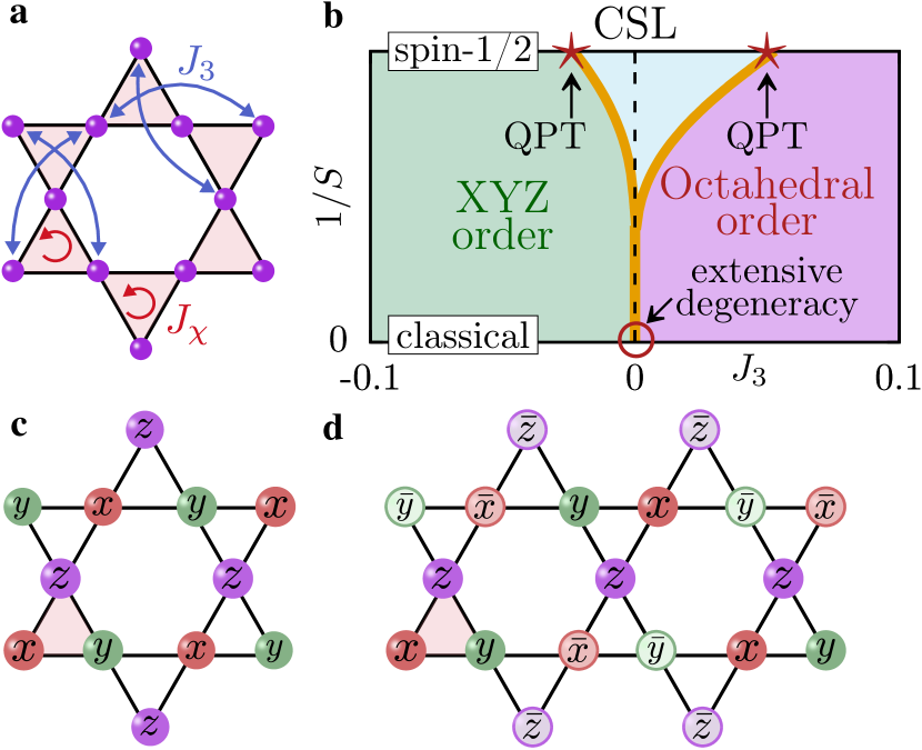
Figure 1: Kagomé lattice. a The chiral three-spin interactions and further neighbor two-spin couplings in the model $H_{\rm spin}$. b Proposed phase diagram of the model $H_{\rm spin}$ as we tune $J_{3}$ and the strength of quantum fluctuations via $1/S$ where $S$ is the spin length. For spin $S\!=\!1/2$, the extensively degenerate classical point evolves into an emergent chiral spin liquid, bounded by non-coplanar magnetic orders. Light blue region indicates where spin-wave fluctuations can destabilize the non-coplanar orders hinting at a quantum spin liquid. c The XYZ umbrella magnetic ordering pattern indicating spins pointing along $x,y,z$. d The Octahedral magnetic ordering pattern with quadrupled unit cell and spins pointing along $(x,\bar{x})$, $(y,\bar{y})$, $(z,\bar{z})$ where $\bar{x}\!\equiv-x$.

In parallel with the interest in such CSLs, there has been a great interest in chiral broken symmetry states in geometrically frustrated systems, which can potentially display nontrivial real-space topology. The most well known examples of these are skyrmion and meron crystals – creating and manipulating such topological textures has important spintronics and information storage applications Nagaosa and Tokura (2013); Fert et al. (2017); Kurumaji et al. (2019); Hirschberger et al. (2019); Hayami et al. (2021); Wang et al. (2022). More recently, chiral density-wave orders have been reported in the metallic kagomé materials AV₃Sb₅ Ortiz et al. (2019); Zhao et al. (2021); Jiang et al. (2021); Khasanov et al. (2022); Neupert et al. (2022), prompting a search for analogous chiral magnetic orders in kagomé magnets such as FeGe Teng et al. (2022), and giving rise to the nascent field of “chiraltronics”.

How are the topologically ordered states such as CSLs related to chiral broken symmetry states with nontrivial real-space topology? Historically, there was an attempt to relate the fractional quantum Hall liquid to a melted Wigner crystal of electrons driven by multi-particle exchanges Kivelson et al. (1987). The analogous question in the field of QSLs is to ask how they arise from the melting of “parent” magnetically ordered states. For instance, gapped $Z_{2}$ QSLs descend from quantum melting of coplanar magnetic orders while preserving topological defects Chubukov et al. (1994). Here, we show that the kagomé lattice CSL is in close proximity to two distinct symmetry breaking orders which feature a uniform and nonzero scalar spin chirality, a nontrivial real-space topological feature they partially share with skyrmion crystals Nagaosa and Tokura (2013); Fert et al. (2017). The scalar chirality is a source of Berry fluxes, which may potentially transmute to background gauge fluxes in an effective gauge theory description of the spin-$1/2$ CSL Wen et al. (1989); Fradkin and Schaposnik (1991); He et al. (2015); Zhang and Li (2021). Our work links a many-body topologically ordered state to the quantum melting of proximate chiral broken symmetry states with nontrivial real-space topology, and shows how both of these ultimately emerge from a highly degenerate manifold of classical chiral states.

Results

Model Hamiltonian and Classical Orders – We consider the kagomé lattice model Hamiltonian

$$H_{\rm spin}=-J_{\chi}\sum_{\bigtriangleup,\bigtriangledown}\mathbf{S}_{i}\cdot\mathbf{S}_{j}\times\mathbf{S}_{k}+J_{3}\sum_{{\mathrel{\rotatebox[origin={c}]{90.0}{$\bowtie$}}\kern-1.54001pt\raisebox{2.71246pt}{$\bullet$}\kern-7.00002pt\raisebox{-2.41112pt}{$\bullet$}}~{}~{}~{}{\mathrel{\rotatebox[origin={c}]{90.0}{$\bowtie$}}\kern-1.54001pt\raisebox{-2.41112pt}{$\bullet$}\kern-7.00002pt\raisebox{2.71246pt}{$\bullet$}}}\mathbf{S}_{i}\cdot\mathbf{S}_{j}.$$ (1)

Fig. 1a shows the chiral three-spin interaction $J_{\chi}$ acting on triangular plaquettes (with spins [$ijk$] ordered anticlockwise), and the $J_{3}$ Heisenberg term coupling farther spins on kagomé bow-ties. Without loss of generality, we fix $J_{\chi}\!=\!1$. Our proposed phase diagram for this model is depicted in Fig. 1b, as we tune $J_{3}$ and the spin length $S$ which controls the degree of quantum fluctuations. It prominently features two distinct chiral broken symmetry orders, and the CSL in the spin-$1/2$ limit.

When $J_{3}\!=\!0$ in Eq. 1, minimizing the energy amounts to maximizing the scalar spin chirality. In the classical limit, where we treat spins as classical unit vectors, this implies that each triangle has spins which must form an orthonormal triad, e.g., going anticlockwise around a triangle, we may have spins pointing along $\{x,y,z\}$. As shown in recent work on the kagomé lattice Pitts et al. (2021), there can be many choices for how to place these triads on adjacent triangles, so this does not uniquely determine the ground state; the number of classical ground states scales as $\Omega\!\sim\!2^{N/3}$ where $N$ is the number of kagomé sites.

However, we see that any nonzero $J_{3}\!<\!0$ completely breaks this degeneracy, selecting a unique ground state (upto global rotations) with XYZ order as shown in Fig. 1c. This XYZ state is a specific member of the family of ${\mathbf{Q}}\!=\!0$ “umbrella states” which have the same unit cell as the original kagomé lattice. In the opposite limit, when $J_{\chi}\!=\!0$, the kagomé lattice decouples into three rhombic sublattices, each of which individually supports ferromagnetic order driven by $J_{3}\!<\!0$. In this limit, introducing an infinitesimal $J_{\chi}$ couples the three sublattices, again leading to XYZ order. The depicted XYZ state can thus be shown to be the unique classical ground state of $H$ for any $J_{3}\!<\!0$ since it separately minimizes each term in the Hamiltonian. A similar analysis indicates that $J_{3}\!>\!0$ leads to antiferromagnetically coupled rhombic sublattices. This selects Octahedral order, with a $12$-site unit cell and zero net magnetization, as the unique classical ground state. Spins in the XYZ state subtend a solid angle $\pi/2$ over elementary triangular plaquettes and trace out $-\pi$ over hexagons. With Octahedral order, spins subtend a solid angle $\pi/2$ over triangular plaquettes and trace out $+\pi$ over hexagons. The XYZ and Octahedral states are ‘regular magnetic orders’ Messio et al. (2011), where lattice symmetries are only broken due to broken spin rotation symmetries; restoring spin rotation symmetry via quantum fluctuations is thus expected to result in symmetric quantum spin liquids.

Quantum Fluctuations – Leading order quantum fluctuations in spin models may be treated using linear spin wave theory (SWT) which is exact to ${\cal O}(1/S)$. To formally treat our model Hamiltonian within SWT, we rescale $J_{\chi}\!\to\!J_{\chi}/(2S)$ in Eq. 1, which leaves the spin-$1/2$ model unchanged but allows the two-spin and three-spin terms to compete in the $S\!\to\!\infty$ limit. We then treat the small fluctuations around the XYZ and Octahedral orders by deriving and solving the bosonic Bogoliubov deGennes SWT Hamiltonian directly in real-space (see Methods). Using this approach, we find that the Octahedral state spectrum admits three exact zero modes, consistent with the expected number of Nambu-Goldstone modes of the fully broken spin rotational symmetry, while the XYZ order admits two zero modes, reflecting the modified count of Nambu-Goldstone modes due to the nonzero net magnetization Watanabe (2020). In addition to these zero modes, there are spin wave modes at nonzero energy; when $J_{3}\!\to\!0$, a macroscopically large number of these excitations descend in energy and merge with the zero modes, reflecting the extensive degeneracy of the classical ground states Pitts et al. (2021).

Dropping the exact zero modes on finite size systems, we have computed the SWT correction to the classical Octahedral and XYZ order parameters and extrapolated the result to the thermodynamic limit; see Supplementary Information (SI) SI for details. We respectively denote these as $M_{\pm}$ for $J_{3}\!>\!0$ and $J_{3}\!<\!0$. These order parameters take the form $M_{\pm}\!=\!S\!-\!\alpha_{\pm}(J_{3})$, where the correction term $\alpha_{\pm}$ depends on $J_{3}$ but is independent of $S$. For small values of $|J_{3}|$, these are well fit by the expressions $\alpha_{\pm}(J_{3})\!=\!c_{\pm}\ln(1/|J3|)$ where $c_{+}\!\approx\!0.068$ and $c_{-}\!\approx\!0.053$; this logarithmic divergence as $J_{3}\!\to\!0^{\pm}$ is consistent with the absence of long-range order at $J_{3}\!=\!0$.

We identify the critical spin value $S_{c}$ where these non-coplanar orders melt for a given $J_{3}$ using an analogue of the well-known Lindemann criterion for melting of crystals. For the magnetic order to melt, we demand that $\alpha_{\pm}(J_{3})\!>\!fS$, where $f$ is a constant. This is equivalent to demanding that the fluctuations exceed a sizeable fraction of the classical ordered moment. Using this, we obtain $1/S_{c}^{(\pm)}\!=\!(f/c_{\pm})/\ln(1/|J_{3}|)$. For $f\!=\!0.4$, we find for spin $S\!=\!1/2$ that this leads to loss of Octahedral order for $0\!<\!J_{3}\!\lesssim\!0.05$ and a breakdown of the XYZ order in the regime $-0.02\!\lesssim\!J_{3}\!<\!0$. In the $S\!=\!1/2$ model, we will see below that this (approximate) window around $J_{3}\!=\!0$ gets replaced by the CSL. Plotting the melting curve for all $S$ leads to the phase boundaries marked in Fig. 1b, which reveals a spin liquid fan emanating from the extensively degenerate classical chiral point.

Parton mean-field theory – To study the phase diagram of this model in the quantum limit of $S\!=\!1/2$, we begin with a Schwinger fermion representation of the spin $\mathbf{S}_{i}\!=\!f^{\dagger}_{i\alpha}\bm{\sigma}^{\phantom{\dagger}}_{\alpha\beta}f^{\phantom{\dagger}}_{i\beta}/2$, with an implicit sum on repeated (Greek) spin indices. Previous DMRG and ED calculations Bauer et al. (2014) on the pure chiral model with $J_{3}\!=\!0$ have shown that it supports a Kalmeyer-Laughlin CSL ground state. Such a CSL is described at the mean-field level in terms of the fermionic “$f$” partons as a topological band insulator with total Chern number $C=2$. This topological insulator is obtained by filling half of the Chern bands formed by a uniform flux piercing elementary triangular plaquettes of the kagomé lattice Ran et al. (2007). To study the impact of $J_{3}$, we recast the spin model in terms of partons

$$H_{\rm parton} = -\sum_{\langle ij\rangle}(t_{ij}f^{\dagger}_{i\alpha}f^{\phantom{\dagger}}_{j\alpha}+t^{*}_{ij}f^{\dagger}_{j\alpha}f^{\phantom{\dagger}}_{i\alpha})$$ (2)

$$+ \frac{J_{3}}{4}~{}\sum_{{\mathrel{\rotatebox[origin={c}]{90.0}{$\bowtie$}}\kern-1.54001pt\raisebox{-2.41112pt}{$\bullet$}\kern-7.00002pt\raisebox{2.71246pt}{$\bullet$}}~{}~{}~{}{\mathrel{\rotatebox[origin={c}]{90.0}{$\bowtie$}}\kern-1.54001pt\raisebox{2.71246pt}{$\bullet$}\kern-7.00002pt\raisebox{-2.41112pt}{$\bullet$}}}~{}f^{\dagger}_{i\alpha}\mathbf{\sigma}_{\alpha\beta}f^{\phantom{\dagger}}_{i\beta}\cdot f^{\dagger}_{j\mu}\mathbf{\sigma}_{\mu\nu}f^{\phantom{\dagger}}_{j\nu}.$$

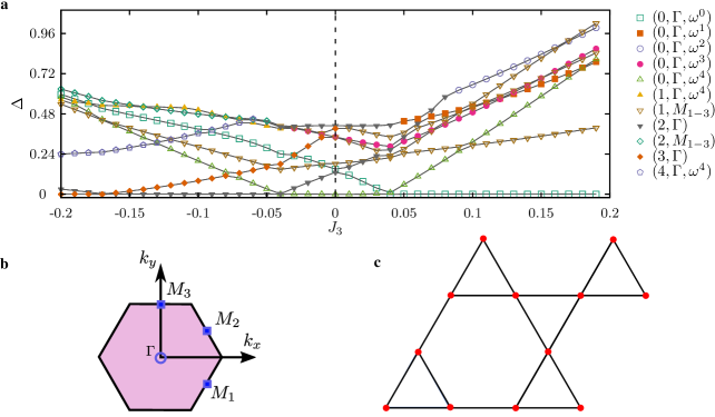
Figure S6: a Energies of eigenstates, relative to the ground state energy, arranged according to the quantum numbers – total spin, momenta ($\Gamma$, $M_{1}$, $M_{2}$, $M_{3}$), and $C_{6}$ rotation (about hexagon centre) eigenvalues at the $\Gamma$ point (with $\omega=e^{\iota\pi/3}$). b The hexagonal Brillouin zone showing the special momentum points related to lattice translational symmetry. c The $12$-site cluster used in the ED calculations, which is also shown in Fig.4 in the main manuscript.

Here, the first term is a kagomé Hofstadter model which captures the mean field description of the CSL at $J_{3}\!=\!0$ Marston and Zeng (1991); Hastings (2000). The complex hoppings $t_{ij}$ are fixed to have equal magnitude $|t_{ij}|\!=\!t$ on all nearest-neighbor bonds, and phases chosen such that the partons experience $\pi/2$-flux around elementary triangular plaquettes and zero-flux around hexagonal plaquettes. This supports Chern bands with total Chern number $C\!=\!2$ (counting both spin-$\uparrow$ and spin-$\downarrow$) at half-filling, providing the correct starting point for the low energy $U(1)_{2}$ Chern-Simons gauge theory description of the CSL Wen et al. (1989). The mean-field spin gap in this insulator is equal to its insulating band gap $\Delta_{mf}\approx\!1.46t$. Matching this to the ED result for the spin gap $\Delta\!\approx\!0.05J_{\chi}$ of the pure chiral model (see Bauer et al. (2014) and Fig. S6 below) fixes $t\!=\!0.034J_{\chi}$. The second term in Eq. 2 is obtained by rewriting the $J_{3}$ spin interaction in Eq. 1 in terms of partons. This Hamiltonian supplemented by a mean-field constraint $\langle f^{\dagger}_{i\alpha}f^{\phantom{\dagger}}_{i\alpha}\rangle\!=\!1$ at each site.

To examine the impact of $J_{3}$, we treat the four-fermion terms using a spatially inhomogeneous and unbiased variational mean-field theory on system sizes upto $108$ sites (see Methods). For small $|J_{3}|$, the gapped Chern insulator is stable to four-fermion interactions. Beyond a critical coupling strength, we find that the internal Weiss fields become nonzero, having a uniform strength ${\cal B}$ and directions which are spatially modulated signifying magnetic symmetry breaking. For $J_{3}\!>\!0.092J_{\chi}$, we find that the converged broken symmetry pattern shows a clear pattern of Octahedral order with a reconstructed $12$-site unit cell ($2\!\times\!2$ kagomé unit cell). For $J_{3}\!<\!-0.077J_{\chi}$, the solution converges to “XYZ” order, i.e. an umbrella state which shares all symmetries of the ${\mathbf{Q}}\!=\!0$ XYZ order, but smoothly interpolates between the XYZ state and the ${\mathbf{Q}}\!=\!0$ coplanar $120^{\circ}$ state. We have also computed the total Chern number of the occupied bands as we tune $J_{3}$ SI . The resulting phase diagram is shown in Fig. 2. Beyond mean-field theory, the broken symmetry insulators are expected to have trivial many-body topology.

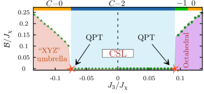
Figure 2: Parton theory phase diagram. Mean field phase diagram of the $S=1/2$ parton theory of Eq. 2 as we vary $J_{3}/J_{\chi}$. For $J_{3}\!>\!0.092J_{\chi}$, we find a phase transition from the mean field CSL into the Octahedral state, while for $J_{3}\!<\!-0.077J_{\chi}$, we find an instability into “XYZ” umbrella order, a state with the same symmetries as the XYZ state. Top line depicts the total Chern number of the half-filled parton bands in various phases as we tune $J_{3}/J_{\chi}$.

Gutzwiller projected wavefunctions – To go beyond parton mean-field theory, and strictly implement the Gutzwiller projection constraint (i.e., exactly one fermion per site), we next turn to a Monte Carlo study of the projected parton wavefunction Hu et al. (2015) to optimize its parameters and study its properties. We consider a parton state $|\Psi_{f}\rangle$ which is obtained as the Slater determinant ground state of a variational Hamiltonian which includes complex nearest neighbor hopping $e^{i\theta_{ij}}$ and next-neighbor hopping $\gamma e^{i\phi_{ij}}$ Hu et al. (2015), with phases chosen to enclose uniform fluxes $\Theta,\Phi$ through elementary and large triangular plaquettes as in Fig.3a. We also include a Weiss field ${\mathbf{b}}_{i}$ via $-\sum_{i}\mathbf{b}_{i}\cdot f^{\dagger}_{i\alpha}\bm{\sigma}^{\phantom{\dagger}}_{\alpha\beta}f^{\phantom{\dagger}}_{i\beta}/2$ to account for magnetic symmetry breaking orders, limiting ourselves to Octahedral order ($J_{3}\!>\!0$) with zero net magnetization; the variational Weiss fields $\mathbf{b}_{i}$ are thus chosen to have an Octahedral pattern as indicated in Fig.3a, with a spatially uniform magnitude $|\mathbf{b}_{i}|\!=\!{\cal B}_{oct}$. We explore the variational ansatz

$$|\Psi_{G}\rangle=\prod_{\mathrel{\rotatebox[origin={c}]{90.0}{$\bowtie$}}}e^{-g\left(S^{z}[~{}{\mathrel{{\rotatebox[origin={c}]{90.0}{$\bowtie$}}\kern-1.25995pt\raisebox{-2.86317pt}{$\bullet$}\kern-3.5pt\raisebox{2.92346pt}{$\bullet$}\kern-7.83998pt\raisebox{2.92346pt}{$\bullet$}\kern-3.64003pt\raisebox{-2.86317pt}{$\bullet$}}}~{}~{}]\right)^{2}}~{}P_{G}|\Psi_{f}\rangle,$$ (3)

where $P_{G}$ denotes Gutzwiller projection to one electron per site. The Gutzwiller wavefunction $P_{G}|\Psi_{f}\rangle$ is supplemented with a product Jastrow correlation factor acting on every kagomé bow-tie, as shown in Fig.3a, where $g$ is the strength of the Jastrow factor and $S^{z}[~{}\mathrel{{\rotatebox[origin={c}]{90.0}{$\bowtie$}}\kern-1.79993pt\raisebox{-4.09024pt}{$\bullet$}\kern-5.0pt\raisebox{4.17638pt}{$\bullet$}\kern-11.19997pt\raisebox{4.17638pt}{$\bullet$}\kern-5.20004pt\raisebox{-4.09024pt}{$\bullet$}}~{}~{}]$ denotes the total $S^{z}$ on the bow-tie excluding the central site. The set of variational parameters explored in our study are $\{\gamma,\Theta,\Phi,g,{\cal B}_{\rm oct}\}$ (see Methods).

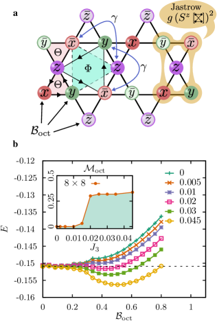
Figure 3: Gutzwiller wavefunction study. a Variational parameters used in our kagomé wavefunction ansatz include a second-neighbor hopping of strength $\gamma$, fluxes $\Theta,\Phi$ through elementary and large triangular plaquettes (shaded), a local Jastrow factor which suppresses the total $S^{z}$ on bow-ties (excluding the central site), and a Weiss field ${\cal B}_{\rm oct}$ which induces Octahedral order; field directions are depicted on the sites. b Variational energy versus ${\cal B}_{\rm oct}$ for an $8\times 8$ lattice for different $J_{3}$, showing a stable CSL state for $J_{3}\!=\!0$ and an instability to Octahedral order for $J_{3}\!\gtrsim\!0.02$. Inset shows the order parameter ${\cal M}_{\rm oct}$ which becomes nonzero in the ordered phase.

For small $J_{3}/J_{\chi}$ of interest, we find that we can get reasonable variational energies by fixing $\Theta\!=\!\pi/2$ and $\gamma\!=\!0.2$ in $H^{\rm var}_{\rm parton}$, and setting the Jastrow strength to $g\!=\!0.045$. We then vary $\Phi,{\cal B}_{\rm oct}$ to explore the variational space for different values of $J_{3}$ (with $J_{\chi}\!=\!1$). For the pure chiral model ($J_{3}\!=\!0$) our wavefunction on an $8\times 8$ kagomé lattice ($192$ spins) yields an energy per site $\simeq-0.151(1)J_{\chi}$; this is somewhat higher than ED ($\approx-0.1729J_{\chi},\ N=36$) and a previous iPEPS study which yield $\approx\!-0.1715J_{\chi}$. Fig. 3b shows the variational energy as a function of ${\cal B}_{\rm oct}$ for various values of $J_{3}$, where we have optimized with respect to $\Phi$ at each point. For $J_{3}\!=\!0$, we find that the CSL is stable towards Octahedral magnetic ordering, but with an apparent local metastable minimum at nonzero ${\cal B}_{\rm tot}$. With increasing $J_{3}$, this metastable minimum rapidly comes down in energy, becoming the true minimum for $J_{3}/J_{\chi}\!\gtrsim\!0.02$, signalling a first-order transition into the Octahedral state. As shown in the inset to Fig. 3b, the Octahedral order ${\cal M}_{\rm oct}\!=\!(1/N)\!\sum_{i}\!\mathbf{m}_{i}\cdot\hat{\mathbf{b}}_{i}$ jumps at this transition. We recognize that a better CSL wavefunction at $J_{3}\!=\!0$ will have lower energy, rendering the CSL more stable and increasing the critical value of $J_{3}$ for the Octahedral instability. We thus turn to a numerical exact diagonalization study to shed further light on the $S\!=\!1/2$ phase diagram.

Exact Diagonalization Results – ED is a powerful unbiased tool to study frustrated kagomé quantum magnets Leung and Elser (1993); Waldtmann et al. (1998); Bauer et al. (2014); Läuchli et al. (2019). To corroborate our results from the preceding sections we have carried out ED calculations for the spin Hamiltonian in Eq. 1 on various finite-size kagomé clusters, shown in Fig. S6f, ranging in size from $N=12$ to $36$.

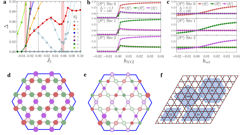
Figure 4: Exact diagonalization results. a Gaps to the lowest lying $S^{z}_{T}=0,\ldots 7$ states for the 36-site cluster. b $\langle S^{\alpha}\rangle$ on adjacent sites taken anticlockwise on any given single up triangle for the $24Rh$-site cluster in a uniform $h_{\rm XYZ}$ field with $J_{3}=-1.4$. c $\langle S^{\alpha}\rangle$ on adjacent sites on a single triangle for the $24$-site cluster in a uniform $h_{\rm oct}$ field with $J_{3}=0.15$. d The induced $\langle S^{\alpha}\rangle$ for the 36-site cluster with a Zeeman field $h_{\rm XYZ}$ applied to a single triangle (shaded) at $J_{3}=-0.5$ and e with a $h_{\rm oct}$ applied to a single triangle (shaded) at $J_{3}=0.1$. The radius of the points are proportional to the overlap with the expected XYZ or Octahedral ordering direction at each site. f The unit cells employed. Note that two different clusters with $N=24$, a rhombic labelled $24Rh$ and a rectangular labelled $24$. The rhombic $N=36$ unit cell is for convenience drawn in its equivalent hexagonal form in d, e, f.

The largest clusters are studied using a fully parallelized Lanczos code that is most optimally used only with the total $S^{z}_{T}$ as a quantum number Läuchli et al. (2011). A full symmetry analysis can be performed on the smaller clusters (see SI SI ). Our results for the spin gaps to the lowest lying states in each $S^{z}_{T}$ sector are shown in Fig. S6a versus $J_{3}$. Two transitions are visible indicated by the shaded red regions. For $J_{3}\!\lesssim\!J^{c}_{\rm XYZ}\!\approx\!-0.03J_{\chi}$ the ground-state transitions away from a singlet and the system becomes ferromagnetic, consistent with the appearance of the XYZ umbrella state. In the vicinity of $J_{3}\!=\!J^{c}_{\rm oct}\!\approx\!0.06J_{\chi}$ the spin gap appears to close signaling a second order transition to a different state. These values of $J^{c}_{3}$ compare favorably to the estimates obtained in our previous analysis. In the CSL-regime for $J^{c}_{\rm XYZ}\!<\!J_{3}\!<\!J^{c}_{\rm oct}$ our results are consistent with a finite spin-gap to the first $S=1$ state above two $S=0$ states.

To identify the magnetically ordered states adjoining the CSL phase we first apply a Zeeman field of the form $-\sum_{\triangle}h_{\rm XYZ}^{\alpha}S^{\alpha}$ on all up-triangles in the lattice, so that each site is counted once. On a single up-triangle with sites numbered (0,1,2), this results in a contribution to the Hamiltonian $-h_{\rm XYZ}(S^{x}_{0}\!+\!S^{y}_{1}\!+\!S^{z}_{2})$. Such a field term will induce the XYZ umbrella state at large $h_{\rm XYZ}$. For the three sites labelled 0,1,2 (anticlockwise) around a single triangle, the response $\langle S^{\alpha}\rangle$ versus $h_{\rm XYZ}$ is shown in Fig. S6b at $J_{3}\!=\!-1.4J_{\chi}$ for the $24Rh$-cluster. Due to the degenerate ground-state at $J_{3}\!=\!-1.4J_{\chi}$ a discontinuous jump in all $\langle S^{\alpha}\rangle$ is observed at $h_{\rm XYZ}\!=\!0$ resulting in a divergent susceptibility with respect to the XYZ umbrella state. In a similar manner we can apply a field term of the form $-\sum_{\triangle}h_{\rm oct}^{\alpha}S^{\alpha}$ for $J_{3}>J^{c}_{\rm oct}$ with $h^{\alpha}_{\rm oct}$ now reflecting the Octahedral ordering shown in Fig. 1d, with a pattern similar to the Weiss field ${\cal B}_{\rm oct}$ used in our variational study. The response of the system to such a field is shown in Fig. S6c versus $h_{\rm oct}$ at $J_{3}\!=\!0.15J_{\chi}$ for the $24$-cluster. (The Octahedral ordering is not compatible with the $24Rh$-cluster). Because of the nonzero spin gap, the response is more gradual, but $\langle S^{\alpha}\rangle$ quickly reach values close to saturation even for small fields. For this value of $J_{3}$ we expect the spin gap to close with $N$. In the limit $h_{\rm oct}\!\to\!0$ we can interpret $\partial\langle S^{\alpha}\rangle/\partial h_{\rm oct}$ as a susceptibility; we have verified that this susceptibility appears to diverge with $N$ SI . On the other hand, if $h_{\rm XYZ}$ or $h_{\rm oct}$ is applied within the CSL, a first order transition to an ordered state is observed at a finite value of the field SI .

To further study the magnetic ordering we apply a finite $h_{\rm XYZ}$ and $h_{\rm oct}$ to a single triangle (shown in shaded red in Fig. S6d,e for the largest $N=36$ cluster and study the induced ordering at the other sites. This breaks most remaining symmetries, necessitating a diagonalization in the full $2^{36}$ dimensional Hilbert space. The results are shown in Fig. S6d,e for $h_{\rm XYZ},h_{\rm oct}=0.4$ at $J_{3}\!=\!-0.5$ and $J_{3}\!=\!0.15$, respectively. The observed patterns are clearly consistent with the XYZ umbrella and Octahedral ordering with only limited decrease in the overlap as one moves away from the triangle where the field is applied (shaded red). We calculate the induced ${\cal M}_{\rm oct}\!=\!0.311$ at $J_{3}\!=\!0.15J_{\chi}$, in good agreement with the Gutzwiller wavefunction result, and ${\cal M}_{\rm XYZ}\!=\!0.443$ at $J_{3}\!=\!-0.5J_{\chi}$. Our ED results unequivocally point to the presence of XYZ and Octahedral orders in close proximity to the CSL.

Discussion

In this work, we have used spin-wave theory, ED, and Gutzwiller wavefunctions, to uncover two chiral magnetic orders – XYZ order and Octahedral order – near the gapped CSL on the kagomé lattice, which are accessed by tuning a small Heisenberg interaction across the bow-ties. Our proposed global phase diagram, as we vary spin $S$, hints at the possibility of unusual QSLs in the chiral model for higher spin, including spin-$1$ magnets, opening up a promising research direction. Previous ED and DMRG calculations have found CSLs and tetrahedral spin crystals on triangular and honeycomb lattices Cincio and Vidal (2013); Hickey et al. (2016); Wietek and Läuchli (2017); Hickey et al. (2017), and complex non-coplanar orders in kagomé lattices with staggered chiral terms which hosts a gapless CSL Oliviero et al. (2021). Our work unveils distinct non-coplanar orders on the kagomé lattice, and points to a universal connection between many-body topological order in the gapped CSL and real-space topology encoded in Berry fluxes of the non-coplanar broken symmetries. Further research is needed to establish such a connection within a field theoretic framework. It would be valuable to extend our work to explore competing orders in models which spontaneously break these symmetries He et al. (2014); Gong et al. (2015), and study the impact of charge doping Jiang and Jiang (2020). Finally, our work lends impetus to extend the exploration of kagome skyrmion materials Hirschberger et al. (2019) to the quantum regime to study the melting of skyrmion crystals as a route to CSLs.

Methods

Spin wave theory To study quantum fluctuations around the XYZ and Octahedral orders, we first perform a local spin rotation $R_{j}$ to align all spins along a global $z-$axis, $\tilde{\bm{S}}_{n,j}=R_{j}\cdot\bm{S}_{n,j}$, where $n$ refers to the magnetic unit cell, and $j$ represents the sub-lattice Tóth and Lake (2015). Expanding the Hamiltonian using Holstein-Primakoff bosons via $\tilde{S}_{n,j}^{+}=\sqrt{2S}~{}b_{n,j},\tilde{S}_{n,j}^{-}=\sqrt{2S}~{}b_{n,j}^{\dagger},\tilde{S}_{n,j}^{z}=S-b_{n,j}^{\dagger}b_{n,j}$, we keep terms upto quadratic order in bosons. Diagonalizing the resulting Bogoliubov deGennes Hamiltonian Colpa (1978); Tóth and Lake (2015) (see SI for details), we calculate the order parameter correction $\alpha\equiv\sum_{n,j}\langle b^{\dagger}_{n,j}b_{n,j}\rangle/N$.

Parton mean-field theory The mean-field calculation for Eq.(2) assumes a uniform flux pattern of $[\pi/2,\pi/2,0]$ through the up, down-triangles, and the hexagons of the kagomé lattice Marston and Zeng (1991); Hastings (2000). The trial Hamiltonian consists of the same nearest-neighbour hopping as ${\mathcal{H}}_{\rm parton}$ while quartic fermion interactions are replaced by complex bow-tie hoppings and independent Zeeman fields on every site. We minimize $\expectationvalue{{\mathcal{H}}_{\rm parton}}$ in the ground state of the trial Hamiltonian, with respect to this large set of mean-field parameters for system sizes upto $108$ kagomé sites for various $J_{3}$. This leads to the spontaneous magnetically ordered states shown in the phase diagram. The corresponding total Chern numbers at half-filling bands Fukui et al. (2005) are also calculated in the converged solution, and shown in Fig.2. The full Chern number phase diagram varying both flux and the Weiss field strength, and details of calculating $\expectationvalue{{\mathcal{H}}_{\rm parton}}$ are given in the SI SI .

Variational Monte Carlo study We use the Metropolis algorithm to stochastically sample spin configurations (typically $\sim 5\times 10^{4}$) in the $S_{z}$ basis in our variational wavefunction $|\Psi_{G}\rangle$ (which is a Slater determinant multiplied by the Jastrow prefactor) in order to calculate the expectation value of the energy. For non-coplanar states, it is convenient to interpret spin-$\uparrow$ and spin-$\downarrow$ as an additional layer coordinate, and the in-plane components of the variational Weiss fields as inter-layer hoppings. To test our optimized chiral wavefunction against previously reported results Hu et al. (2015), we generalized the spin model $H_{\rm spin}$ to incorporate a nearest-neighbor Heisenberg exchange term with strength $J_{1}$, and explored different values of $(J_{1},J_{3},J_{\chi})$. (i) For $J_{3}\!=\!0$ and $J_{\chi}\!=\!0.15J_{1}$, our optimal wavefunction yields an energy per site $\approx\!-0.445(1)J_{1}$, quite close to a previous careful VMC study of the model Hu et al. (2015) which found $\approx\!-0.450J_{1}$. (ii) On the $12$-site kagomé cluster, ED for the pure chiral model (i.e., $J_{3}\!=\!J_{1}\!=\!0$) yields a singlet ground state, with energy per spin $\approx\!-0.186221J_{\chi}$, while our $12$-site spin liquid wavefunction yields $\approx\!-0.176(1)J_{\chi}$ per spin. For comparison, ED on the 36-site cluster at $J_{3}=0$ yields $\approx\!-0.172852J_{\chi}$.

Exact Diagonalization Numerical exact diagonalization (ED) were performed using a fully parallelized Lanczos code using an on-the-fly calculation of the action of the Hamiltonian matrix. Clusters used in the calculations are shown in Fig. S6f. The full symmetry analysis of the spectrum was done on a smaller, $12-$site system, and the $C_{6}$ rotation eigenvalues of the lowest two singlets was found to be consistent with earlier studies Cincio and Vidal (2013). Further details are presented in the Supplementary Information (SI) SI .

Supplementary Information is available in the online version of the paper.

Acknowledgements

This work was supported by the Natural Sciences and Engineering Research Council of Canada. This research was enabled in part by support provided by Sharcnet (www.sharcnet.ca) and Compute Canada (www.computecanada.ca).

Author Contributions

Exact diagonalization calculations were performed by E.S.S and A.B. Spin wave and parton mean field calculations were carried out by A.B. and A.H. The Gutzwiller Monte Carlo simulations were done by A.P. and A.H. A.P. planned and supervised the project. All authors contributed to the writing of the manuscript.

Author Information

The authors declare no competing financial interests. Correspondence should be addressed to A.P. (arun.paramekanti@utoronto.ca).

Data availability

The data that support the findings of this study are available from the corresponding author upon reasonable request and will later be made available on github.

Code availability

The computer codes used to generate the data used in this study are available from the corresponding author upon reasonable request.

Supplementary Information:

Chiral Broken Symmetry Descendants of the Kagomé Lattice

Chiral Spin Liquid

Anjishnu Bose¹, Arijit Haldar¹, Erik S. Sørensen², and Arun Paramekanti¹

¹Department of Physics, University of Toronto, 60 St. George Street, Toronto, ON, M5S 1A7 Canada

²Department of Physics, McMaster University, 280 Main St. W., Hamilton ON L8S 4M1, Canada

S1 Spin Wave theory

To find the linear spin-wave dispersion, we first have to rotate each spin within a unit cell to the $\hat{z}$ direction. We can define three useful unit vectors quantities from the local rotation matrix $R_{j}$ which rotates the ordered spin vector $\mathbf{S}_{j}\to\hat{z}$ Tóth and Lake (2015), namely

$$\begin{gathered}u_{j}^{\alpha}=R_{j}^{\alpha 1}+\iota R_{j}^{\alpha 2}\,,\>\>\>\bar{\bm{u}}_{j}=\bm{u}_{j}^{*}\,,\>\>\>v_{j}^{\alpha}=R_{j}^{\alpha 3}\,.\end{gathered}$$ (S1.4)

Here $j$ refers to the basis site within the magnetic unit cell, and $\alpha$ labels vector components, and superscripts $1,2,3$ refer to columns of the rotation matrix. In terms of these, we can write the original spin operators as

$$S_{n,j}^{\alpha}=\frac{1}{2}\left(u_{j}^{\alpha}\tilde{S}_{n,j}^{-}+\bar{u}_{j}^{\alpha}\tilde{S}_{n,j}^{+}\right)+v_{j}^{\alpha}\tilde{S}_{n,j}^{z}$$ (S1.5)

Finally, we use the Holstein-Primakoff transformation as given in the main text as

$$\begin{gathered}\tilde{S}_{n,j}^{+}=\sqrt{2S}\>b_{n,j}\,,\\ \tilde{S}_{n,j}^{-}=\sqrt{2S}\>b_{n,j}^{\dagger}\,,\\ \tilde{S}_{n,j}^{z}=S-b_{n,j}^{\dagger}b_{n,j}\,.\\ \end{gathered}$$ (S1.6)

and end up with

$$S_{n,j}^{\alpha}=\sqrt{\frac{S}{2}}\left(\bar{u}_{j}^{\alpha}b_{n,j}+u_{j}^{\alpha}b_{n,j}^{\dagger}\right)+v_{j}^{\alpha}\left(S-b_{n,j}^{\dagger}b_{n,j}\right)$$ (S1.7)

S1.1 Chiral Hamiltonian

We start with the pure chiral Hamiltonian on the kagomé lattice as

$${\mathcal{H}}_{\chi}=-\sum_{m,n,p}\sum_{i,j,k}J^{ijk}_{mnp}\>\bm{S}_{m,i}\cdot\left(\bm{S}_{n,j}\times\bm{S}_{p,k}\right)\,,$$ (S1.8)

where $m,n,p$ mark the magnetic unit cell (quadrupled unit cell as compared to the normal kagomé), and $i,j,k\in\{0,1,2,...,11\}$ for the Octahedral order, whereas $i,j,k\in\{0,1,2\}$ for the XYZ order, mark the sublattices. $J^{ijk}_{mnp}$ is chosen such that each up and down triangle is summed over once; this coupling constant will be chosen to be $J_{\chi}$. After substituting back (S1.7) into (S1.8), and only keeping terms upto quadratic order (also ignoring linear terms since their expectation vanishes), we end up with

$$\begin{split}{\mathcal{H}}_{\chi}=-\sum_{m,n,p}\sum_{i,j,k}J^{ijk}_{mnp}\>\bigg{\{}\frac{S^{2}}{2}\bigg{[}\bigg{(}&b_{n,j}b_{p,k}\left(\bm{v}_{i}\cdot\bar{\bm{u}}_{j}\times\bar{\bm{u}}_{k}\right)+b_{n,j}b_{p,k}^{\dagger}\left(\bm{v}_{i}\cdot\bar{\bm{u}}_{j}\times\bm{u}_{k}\right)\\ +&b_{n,j}^{\dagger}b_{p,k}\left(\bm{v}_{i}\cdot\bm{u}_{j}\times\bar{\bm{u}}_{k}\right)+b_{n,j}^{\dagger}b_{p,k}^{\dagger}\left(\bm{v}_{i}\cdot\bm{u}_{j}\times\bm{u}_{k}\right)\bigg{)}\\ +&\{\text{cyclic permutations}\}\bigg{]}\\ +\left(\bm{v}_{i}\cdot\bm{v}_{j}\times\bm{v}_{k}\right)\bigg{[}&S^{3}-S^{2}\left(b_{m,i}^{\dagger}b_{m,i}+b_{n,j}^{\dagger}b_{n,j}+b_{p,k}^{\dagger}b_{p,k}\right)\bigg{]}\bigg{\}}\end{split}$$ (S1.9)

S1.2 Bow-tie Heisenberg Hamiltonian

The bow-tie Heisenberg Hamiltonian looks like

$${\mathcal{H}}_{bt}=\frac{1}{2}\sum_{m,n}\sum_{i,j}J_{m,n}^{i,j}\>\bm{S}_{m,i}\cdot\bm{S}_{n,j}\,.$$ (S1.10)

where the factor of $1/2$ is because we will be using the symmetric form of $J_{m,n}^{i,j}=J_{n,m}^{j,i}$, and $J$ is chosen such that we sum over each bow-tie pair once, and we will fix this coupling constant to be $J_{3}$. Again, repeating the steps as before, dropping terms higher order than quadratic in the boson operators, and also ignoring the linear terms, we end up with

$$\begin{split}{\mathcal{H}}_{bt}=\sum_{m,n}\sum_{i,j}\frac{J_{m,n}^{i,j}}{2}\>\bigg{\{}\frac{S}{2}\bigg{[}&b_{m,i}b_{n,j}(\bar{\bm{u}}_{i}\cdot\bar{\bm{u}}_{j})+b_{m,i}b_{n,j}^{\dagger}(\bar{\bm{u}}_{i}\cdot\bm{u}_{j})+b_{m,i}^{\dagger}b_{n,j}(\bm{u}_{i}\cdot\bar{\bm{u}}_{j})+b_{m,i}^{\dagger}b_{n,j}^{\dagger}(\bm{u}_{i}\cdot\bm{u}_{j})\bigg{]}\\ +(\bm{v}_{i}\cdot\bm{v}_{j})\bigg{[}&S^{2}-S\bigg{(}b_{m,i}^{\dagger}b_{m,i}+b_{n,j}^{\dagger}b_{n,j}\bigg{)}\bigg{]}\bigg{\}}\,.\end{split}$$ (S1.11)

S1.3 Bogoliubov deGennes (BdG) Hamiltonian

Combining the two as ${\mathcal{H}}=1/(2S)\cdot{\mathcal{H}}_{\chi}+{\mathcal{H}}_{bt}$, we end up with a BdG Hamiltonian. To diagonalize it, we first have to ensure that the Hamiltonian is positive definite. In our case, it is actually positive semi-definite due to the existence of Goldstone modes. The number of Goldstone modes depends on the ordering Watanabe (2020) which can be seen in the formula as

$$n_{GM}=n_{BG}-\frac{1}{2}{\mathrm{Rank}}(\rho)\,,$$ (S1.12)

where $n_{GM}$ is the number of Goldstone modes, $n_{BG}$ is the number of broken generators. Furthermore,

$$\rho^{ab}=\frac{1}{V}f^{abc}\expectationvalue{Q^{c}}\,,$$ (S1.13)

where $V$ is the volume of the system, $f^{abc}$ are the structure constants of the symmetry group being broken, and $Q^{c}$ are the generators of the global symmetry. For a model on a lattice, $V=N$, the number of sites. Since the symmetry group being broken in our case is $SU(2)$ spin-rotation symmetry, we also have that $f^{abc}=\epsilon^{abc}$, and $Q^{c}=\sum_{i=1}^{N}S_{i}^{c}$.

On the ferromagnetic side with the XYZ ordering, $\expectationvalue{Q^{c}}=S\frac{N}{3}$, for each of $c=x,y,z$ because we will have $N/3$ spin$-S$ pointing along the three orthogonal directions. This gives ${\mathrm{Rank}}(\rho)=2$. However, since XYZ ordering completely breaks all spin-rotational symmetries, $n_{BG}=3$. Hence using Eq. S1.12, we find that $n_{GM}^{\mathrm{XYZ}}=2$. In our BdG Hamiltonian, we find twice this number of zero eigenvalues ($2n_{GM}=4$) providing a consistency check.

On the antiferromagnetic side, with the Octahedral order, all the symmetries are again broken. At the same time, this ordering has $\expectationvalue{Q^{c}}=0$ for any $c=x,y,z$ and hence $n_{GM}=n_{BG}=3$). In our BdG Hamiltonian, we find twice this number of zero eigenvalues ($2n_{GM}=6$) providing a consistency check.

Lastly, we find that at the pure chiral point, the number of zero modes scale with the system size if we start with Octahedral or XYZ order, as is expected from the classical analysis as given in Pitts et al. (2021). However, since we are looking at fluctuations around potentially stable and unique ground states, we will consider the limit $J_{3}\to 0^{\pm}$ and not the pure chiral point with $J_{3}=0$.

Since our analysis was done in real space, we get rid of the zero modes by adding small random diagonal terms to the Hamiltonian of the order $\sim 10^{-10}$. Doing this also helps break degeneracies, which is essential for obtaining the BdG wavefunctions correctly Colpa (1978). After that is done, we end up in a basis $(\gamma_{i},...,\gamma^{\dagger}_{i},...)$ s.t. ${\mathcal{H}}=2\sum_{i}\epsilon_{i}\left(\gamma^{\dagger}_{i}\gamma_{i}\right)+\epsilon_{0}$, where $\epsilon_{0}$ is some constant energy shift which we can safely ignore. This new basis is related to the original basis through a similarity transformation, $P$ (not a unitary transformation). Now we are interested in the expectation value, $\alpha\equiv\frac{1}{N}\sum_{n,j}\expectationvalue{b^{\dagger}_{n,j}b_{n,j}}$. We can write $\alpha$ as a linear combination of $\expectationvalue{\gamma^{\dagger}_{i}\gamma_{j}}\,,\expectationvalue{\gamma_{i}\gamma^{\dagger}_{j}}\,,\expectationvalue{\gamma_{i}\gamma_{j}},\expectationvalue{\gamma^{\dagger}_{i}\gamma^{\dagger}_{j}}$ and some factors coming from $P$. However, in the ground state, the only non-zero expectation is that of $\expectationvalue{\gamma_{i}\gamma^{\dagger}_{j}}=\delta_{ij}$, all the rest vanish.

Doing this procedure for both the Octahedral and the XYZ ordering gives us $\alpha_{\pm}$ where $\pm$ denotes the anti-ferromagnetic and the ferromagnetic cases. The finite size scaling of $\alpha_{\pm}(L)$ versus system size for $J_{3}<0$ is shown in Fig. S1 for two different values of $J_{3}$. For small $|J_{3}|$, the fluctuations decrease with $L$ while for larger $|J_{3}|$ they increase with $L$, in both cases extrapolating to a finite value as $L\to\infty$ when $J_{3}\neq 0$. Fig. S2 shows similar finite size scaling plots for $J_{3}>0$. From these plots, we extract the thermodynamic limit value of $\alpha_{\pm}(J_{3})$.

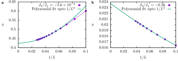
Figure S1: $\alpha$ vs $1/L$ for the ferromagnetic XYZ ordering, at different values of $|J_{3}/J_{\chi}|$.

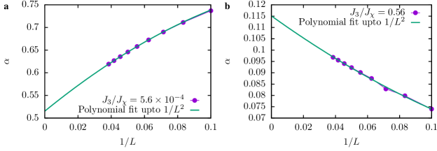
Figure S2: $\alpha$ vs $1/L$ for the anti-ferromagnetic Octahedral ordering, at different values of $|J_{3}/J_{\chi}|$.

Fig. S3 shows the thermodynamic limit extrapolated value of $\alpha_{\pm}$ for both signs of $J_{3}$. The $x$-axis is shown in a log scale to emphasize that $\alpha_{\pm}=c_{\pm}\cdot\log\left(1/|J_{3}|\right)$ for small values of $|J_{3}|$ (with $J_{\chi}$ fixed to 1). This logarithmic divergence as we approach the pure chiral Hamiltonian is consistent with the idea that long range order is completely melted away for all spins at $J_{3}=0$. Furthermore, to estimate where the order melts for finite $S$, we have to come up with a definition s.t. the value of $|J_{3}|$ when $\alpha_{\pm}\left(|J_{3}|\right)=f\cdot S\,,\>\>\>0<f<1$, is the value where the ordering melts away for the spin, $S$. The value of $f$ which gives results matching semi-quantitatively with our ED data comes to about $f\approx 0.4$.

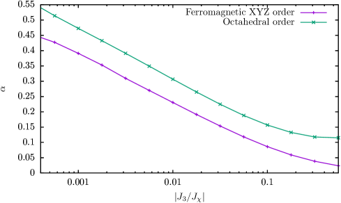
Figure S3: $\alpha\equiv\frac{1}{N}\sum_{n,j}\expectationvalue{b^{\dagger}_{n,j}b_{n,j}}$ vs $|J_{3}/J_{\chi}|$ for the ferromagnetic XYZ ordering, and the Anti-ferromagnetic Octahedral ordering.

S2 Parton mean-field theory

S2.1 Operator expectation values

We start by writing the spin operator in terms of the spin-$1/2$ Schwinger fermion operators as

$$\bm{S}_{i}=\frac{1}{2}f_{i}^{\alpha\dagger}\bm{\sigma}_{\alpha\beta}f_{i}^{\beta}\,.$$ (S2.14)

In terms of these partons, the trial or the variational mean field Hamiltonian looks as follows

$$\begin{split}{\mathcal{H}}_{trial}=-&\sum_{i,j}t_{ij}\sum_{\alpha}\left(e^{-\iota\phi_{ij}}f_{i}^{\alpha\dagger}f_{j}^{\alpha}+e^{\iota\phi_{ij}}f_{j}^{\alpha\dagger}f_{i}^{\alpha}\right)-\sum_{i}f_{i}^{\alpha\dagger}\left(\bm{\hat{b}}_{i}.\bm{\sigma}\right)_{\alpha\beta}f_{i}^{\beta}\,.\end{split}$$ (S2.15)

Then, the expectation of the physical Hamiltonian is calculated in the ground state of such a variational Hamiltonian. Now since the variational Hamiltonian is just a free theory, the expectation of any operator can be written entirely in terms of two-point correlations through Wick’s theorem. The two point correlations for the trial Hamiltonian are defined as

$$\chi_{ij}^{\alpha\beta}\equiv\expectationvalue{f_{i}^{\alpha\dagger}f_{j}^{\beta}}\,,\>\>\>\chi_{ii}^{\alpha\alpha}\equiv\expectationvalue{n_{i}^{\alpha}}\,.$$ (S2.16)

Also note that, in general, $\chi_{ij}^{\alpha\beta}$ is not proportional to $\delta^{\alpha\beta}$ because of the Weiss field which mixes the two spins. Focusing on the Heisenberg like interaction term, we find that the relevant expectation value of the four-fermion operators looks like

$$\begin{split}\expectationvalue{f_{i}^{\alpha\dagger}f_{i}^{\beta}f_{j}^{\mu\dagger}f_{j}^{\nu}}&=\expectationvalue{f_{i}^{\alpha\dagger}f_{i}^{\beta}}\expectationvalue{f_{j}^{\mu\dagger}f_{j}^{\nu}}-\expectationvalue{f_{i}^{\alpha\dagger}f_{j}^{\nu}}\expectationvalue{f_{j}^{\mu\dagger}f_{i}^{\beta}}\\ &=\chi_{ii}^{\alpha\beta}.\chi_{jj}^{\mu\nu}-\chi_{ij}^{\alpha\nu}.\chi_{ji}^{\mu\beta}\,,\end{split}$$ (S2.17)

where the relative $-$ sign appears because of fermion anti-commutation relation. We therefore get that

$$\begin{split}\expectationvalue{\bm{S}_{i}.\bm{S}_{j}}&=\frac{1}{4}\sigma^{a}_{\alpha\beta}\sigma^{a}_{\mu\nu}\left[\chi_{ii}^{\alpha\beta}.\chi_{jj}^{\mu\nu}-\chi_{ij}^{\alpha\nu}.\chi_{ji}^{\mu\beta}\right]\\ &=\frac{1}{4}\left(2\delta_{\alpha\nu}\delta_{\beta\mu}-\delta_{\alpha\beta}\delta_{\mu\nu}\right)\left[\chi_{ii}^{\alpha\beta}.\chi_{jj}^{\mu\nu}-\chi_{ij}^{\alpha\nu}.\chi_{ji}^{\mu\beta}\right]\\ &=\frac{1}{4}\left(2\Tr(\chi_{ii}\>\chi_{jj})-\Tr(\chi_{ii}).\Tr(\chi_{jj})\right)-\left(2\Tr(\chi_{ij}).\Tr(\chi_{ji})-\Tr(\chi_{ij}\>\chi_{ji})\right)\,,\end{split}$$ (S2.18)

where we have used the completeness relation for Pauli matrices.

S2.2 Phase diagram and Chern numbers

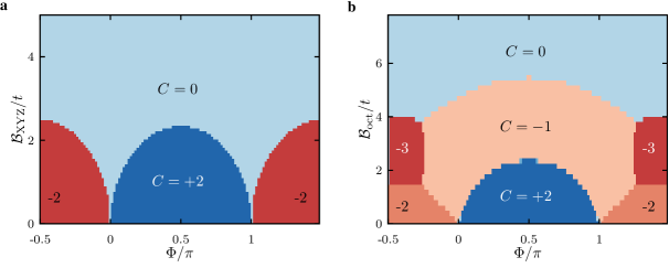
Figure S4: Chern number phase diagram for the ferromagnetic (a) and the anti ferromagnetic (b) cases obtained using parton mean-field theory.

The Chern number Fukui et al. (2005) phase diagrams are obtained using Eq. (S2.15) with the hopping being restricted to nearest neighbours at unit strength. The flux pattern is varied s.t. there is a flux of $\Phi$ through each up and down-triangle, and a flux of $\pi-2\Phi$ through each hexagon of the kagomé lattice. Lastly, an ordering is chosen for the Weiss fields, but its strength, $\mathcal{B}$, is varied. The ordering is chosen from our mean field results, when we optimize the total energy for the Chern insulator after switching on bow-tie Heisenberg interactions. In the main manuscript, we have shown the Chern number evolution in Fig. 2 at fixed $\Phi/\pi=0.5$, fixed by the effective Hofstadter model, and the spontaneously induced ${\cal B}$.

For the antiferromagnetic case, the ordering turns out to be Octahedral after a critical value of $J_{3}=J_{3}^{\mathrm{oct}}>0$, while for the ferromagnetic case, below a critical negative value of $J_{3}=J_{3}^{\mathrm{XYZ}}<0$, the ordering is that of a squished XYZ state, which interpolates between perfect XYZ order and the $Q=0$, $120^{\circ}$ coplanar state. We are calling this the “XYZ” state since it is an umbrella order with the same symmetries as the XYZ state.

S3 Exact Diagonalization

The unit cells we have used for performing exact diagonalizations (ED) are shown in Fig. 4f in the main paper. On a regular lattice every site participates in two unique bow-tie couplings. In order to compare results for the different size unit cells, care has to be taken when implementing the periodic boundary conditions on the $N=12$ and $N=24$ rectangular clusters. For the $N=12$ cluster, all bow-tie bonds can connect both ways around the torus and are therefore counted twice. For the $N=24$ cluster, there are 8 such bow-tie bonds that connect both ways around the small circumference of the torus and are therefore counted twice, while the remaining bow-tie bonds are only counted once. For the rhombic $N=24Rh$ unit cell as well as for the $N=36$ cell, all the $2N$ bow-tie bonds are uniquely defined with periodic boundary conditions and are only counted once.

S3.1 Phase Diagram

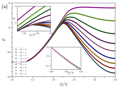
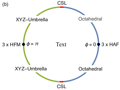
Figure S5: (a) Total energy versus $\phi/\pi$ for the $N=24Rh$ unit cell. The insets show close up behavior in the vicinity of $\phi=\pi$ and $\phi=3\pi/2$. Note that the $S^{z}_{T}=8$ state is not degenerate with $S_{T}^{z}$ until $\phi=\pi$. (b) Phase diagram as a function of $\phi$. The extent of the CSL phase is estimated from the $N=36$ results in the main paper. For $\phi=0,\pi$ the system decouples into 3 separate lattices.

To gain a more complete understanding of the phase diagram we parameterize the couplings in $H_{\rm spin}$ in the following way:

$$H_{\phi}=\sin(\phi)\sum_{\bigtriangleup,\bigtriangledown}\mathbf{S}_{i}\cdot\mathbf{S}_{j}\times\mathbf{S}_{k}+\cos(\phi)\sum_{{\mathrel{\rotatebox[origin={c}]{90.0}{$\bowtie$}}\kern-1.54001pt\raisebox{2.71246pt}{$\bullet$}\kern-7.00002pt\raisebox{-2.41112pt}{$\bullet$}}~{}~{}~{}{\mathrel{\rotatebox[origin={c}]{90.0}{$\bowtie$}}\kern-1.54001pt\raisebox{-2.41112pt}{$\bullet$}\kern-7.00002pt\raisebox{2.71246pt}{$\bullet$}}}\mathbf{S}_{i}\cdot\mathbf{S}_{j}.$$ (S3.19)

With this parameterization we can explore the full phase diagram of the model, reaching the limits of $J_{\chi}=0\ (\phi=0,\pi)$ described by the 3 lattice toy model from section S3.6 at $\phi=\pi$. We first note that this model is invariant under $\phi\to 2\pi-\phi$ which leaves $\cos(\phi)$ and thereby the nearest neighbor Heisenberg term unchanged but changes the sign of the chiral term. However, it is easy to see that the chiral interaction is independent of the sign implying the invariance. Strictly speaking we therefore only need to consider $\phi\in(0,\pi)$ or equivalently $\phi\in(\pi,2\pi)$.

The lowest energy for each of the sectors $S_{T}^{z}=0\ldots 8$ for the $N=24Rh$ lattice are shown in Fig. S5(a) for $\phi\in(\pi,2\pi)$ with the insets showing detailed behavior close to $\phi=\pi$ and $3\pi/2$. The spectrum is mostly dominated by the nearest neighbor Heisenberg coupling leaving only a small region close to $\phi=\pi/2,3\pi/2$ (estimated from the 36-site results in the main paper) for the CSL (see upper inset in Fig. S5(a)). On the ferromagnetic side, $\pi/2<\phi<3\pi/2$, and close to $\phi=\pi$, the second inset shows that a gap remains to the $S^{z}_{T}=8$ state until the completely decoupled lattices are reached at $\phi=\pi$. This is consistent with the prediction of $S_{T}=7$ for the ground-state in this limit obtained from the toy model (section S3.6). In a similar manner we expect that we reach 3 decoupled anti-ferromagnetic nearest neighbor lattices only precisely at $\phi=0$ with the preceding phase being characterized by Octahedral ordering. A sketch of the expected phase-diagram is shown in Fig. S5(b).

S3.2 Spectrum with quantum numbers

We restrict a more complete symmetry analysis, including more quantum numbers than the $S^{z}_{T}$ used in the main paper, to the small $N=12$ cluster ($2\times 2$ kagomé unit cells).

For $J_{\chi}\!=\!1$ and $J_{3}\!=\!0$, i.e., the pure chiral model, the ground state energy per site is $\approx\!-0.186J_{\chi}$. This ground state is a spin singlet at the $\Gamma$-point ${{\bf{k}}}=(0,0)$, but it has a non-trivial $C_{6}$ eigenvalue for $2\pi/6$ rotations about the kagomé hexagon centre, with $\lambda^{(1)}_{0}(C_{6})=e^{i4\pi/3}$. The next singlet in the spectrum is also a $\Gamma$-singlet but with rotation eigenvalue $\lambda^{(2)}_{0}(C_{6})=1$. We expect these two singlets, which are separated by a gap $\sim\!0.151J_{\chi}$ on our small system size, to become the two topologically degenerate levels of the CSL in a large system; indeed, these rotation eigenvalues are consistent with what we would obtain from the $S$ and $T$ matrices for the Abelian anyons (semions) of the CSL Cincio and Vidal (2013). For the $N=12$ cluster the second singlet is higher in energy than the first triplet at $J_{3}=0$. For the $N=36$ cluster in Fig 4a in the main paper it appears below the triplet at $J_{3}=0$ consistent with our expectation that it becomes degenerate with the ground-state singlet in the thermodynamic limit.

With increasing bow-tie exchange $J_{3}$, we find that the energy of one of these singlets decreases while the other singlet drifts up in energy. At the same time, a set of triplets, with momenta at the $M$-points of the hexagonal Brillouin zone (BZ), come down in energy. We tentatively identify the point where the upward drifting singlet crosses the downward moving $M$-triplet, which occurs at $J_{3}/J_{\chi}\approx 0.1$, as a CSL to magnetic order transition point. This is in qualitative agreement with the estimate of $J_{3}/J_{\chi}\approx 0.06$ for the $N=36$ cluster discussed in the main paper.

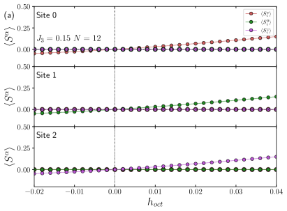
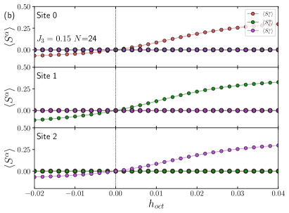
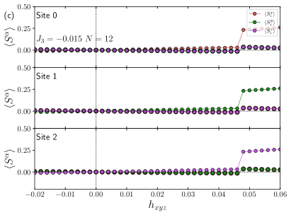
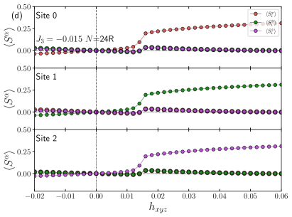
Figure S7: $\langle S^{a}\rangle$ on subsequent sites around a triangle for the $N=12$ unit cell at $J_{3}=0.15$ for (a) $N=12$ and (b) $N=24$ versus applied field $h_{\mathrm{oct}}$ and, for $J_{3}=-0.015$ for (c) $N=12$ and (d) $N=24Rh$ versus applied field $h_{\mathrm{XYZ}}$.

S3.3 Response to global $h_{\mathrm{XYZ}}$ and $h_{\mathrm{oct}}$ fields

As discussed in the main paper, we consider the response of the system to global Zeeman fields $h_{\mathrm{XYZ}}$ and $h_{\mathrm{oct}}$ inducing the XYZ-umbrella and Octahedral orderings. In Fig. S7 we show additional results. Fig. S7(a),(b) illustrate the behavior of the system at $J3=0.15$ where Octahedral ordering is present when the system size is increased from (a) $N=12$ to (b) $N=24$. (Fig. S7(a) is identical to Fig. 4c in the main paper.) Since the field is applied throughout the lattice we an limit our analysis to a single triangle with adjacent sites labelled 0,1,2 (anti clock-wise). As is clearly observed in Fig. S7(a),(b) the response is significantly stronger for $N=24$ and if a susceptibility, $\partial\langle S^{\alpha}\rangle/\partial h_{\mathrm{oct}}$ with respect to $h_{\mathrm{oct}}$ is defined we would expect it to diverge with $N$ at zero applied field ($h_{\mathrm{oct}}=0$), consistent with the presence of Octahedral ordering.

It is also instructive to analyze the response to XYZ-umbrella ordering within the CSL phase. From the results presented in the main paper we know that for $J_{3}\lesssim-0.03J_{\chi}$ the ordering spontaneously jumps to large values for any finite field. In Fig. S7(c),(d) we show results at $J_{3}=-0.015J\chi$ within the CSL phase for (c) $N=12$ and (d) $N=24Rh$ versus applied field $h_{\mathrm{XYZ}}$. The onset is again abrupt but now appears at finite field strengths. Since we do not expect the spin gap to close completely in the CSL phase we expect that a finite field will always be needed to induce the XYZ-umbrella ordering even though the gap decreases noticeable between $N=12$ and $N=24Rh$ as reflected in the shift in the onset of ordering from $h_{\mathrm{XYZ}}\approx 0.048$ to $h_{\mathrm{XYZ}}\approx 0.014$.

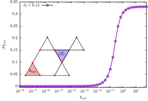
Figure S8: The overlap of induced magnetization at $J_{\chi}=1\,,J_{3}=0.15$ with the expected Octahedral pattern on the blue triangle, different from the one where a Zeeman field is applied (orange triangle), with strength $h_{\mathrm{oct}}$ for $N=12$ versus $h_{\mathrm{oct}}$.

S3.4 Induced magnetization from local $h_{\mathrm{oct}}$ and $h_{\mathrm{XYZ}}$ fields

As explained in the main paper, it is instructive to examine the nature of magnetic ordering induced by a local Zeeman field applied around a single triangle by introducing a term in the spin Hamiltonian of the form $-h_{\mathrm{oct}}\left(S^{z}_{0}+S^{x}_{1}+S_{2}^{y}\right)$. The field then points along $\hat{z}$, $\hat{x}$, and $\hat{y}$ respectively at the three adjacent sites $i=0,1,2$ around the triangle and the response can be studied throughout the lattice as the field is varied. The introduction of $h_{\mathrm{oct}}$ completely break all the spin and lattice symmetries, and will mix the ground state with the low-lying states. Note that there is no need to introduce a field on more than 3 sites to uniquely induce the Octahedral ordering. The introduction of a local $h_{\mathrm{XYZ}}$ field is identical in form.

We have computed the resulting induced moments at all sites $\langle\mathbf{S}_{i}\rangle$ on the cluster. We then choose a triangle furthest away from the one where the Zeeman field is applied, and calculate the overlap, $\mathcal{M}_{\mathrm{oct}}$ of the induced magnetization on this triangle with the expected Octahedral pattern, and plot it as a function of the Zeeman field strength. This is shown in Fig. S8.

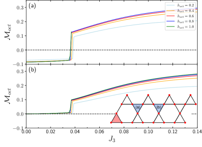
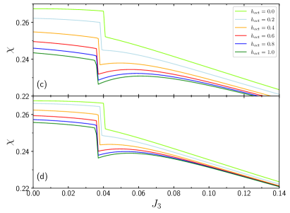
Figure S9: (a), (b) The overlap, $\mathcal{M}_{\mathrm{oct}}$ of induced magnetization with the expected Octahedral pattern versus $J_{3}$ for a range of field strengths $h_{\mathrm{oct}}=0.2,0.4,0.6,0.8,1.0$ shown for two different triangles (blue shaded). The field is applied on the red triangle. A regular $N=24$ unit lattice was used. (c), (d) The scalar chirality $\chi=\langle\mathbf{S}_{i}\cdot(\mathbf{S}_{j}\times\mathbf{S}_{k})\rangle$ around the same two triangles as shown in panels (a), (b).

To further explore how the Octahedral ordering is induced we have repeated the calculation of $\mathcal{M}_{\mathrm{oct}}$ of the $N=24$ site lattice as a function of $J_{3}$ (with $J_{\chi}=-1$) for a range of field strengths $h_{\mathrm{oct}}=0.2,0.4,0.6,0.8,1.0$. Our results are shown in Fig. S9. The field is again applied only at a single triangle shown in red in Fig. S9 while $\mathcal{M}_{\mathrm{oct}}$ is calculated on two different triangles shown in blue. Panel (b) corresponds to the triangle furthest away from the red triangle. Clearly the Octahedral pattern appears rapidly at even modest applied fields for sufficiently large $J_{3}$. For $J_{3}\lesssim 0.04$ the CSL phase is clearly visible and the Octahedral order is absent. For this $N=24$ the transition between the CSL and the Octahedral ordered phase appears first order at finite field.

For comparison, it is instructive to study the behavior of scalar chirality $\chi=\langle\mathbf{S}_{i}\cdot(\mathbf{S}_{j}\times\mathbf{S}_{k})\rangle$ on the same triangles as $J_{3}$ is varied. This is shown in Fig. S9(c),(d). The transition between the CSL and Octahedral phase is again clearly visible. For $h_{\mathrm{oct}}=0$ $\chi$ is uniform among all triangles in the lattice. Note that, as the applied Octahedral field $h_{\mathrm{oct}}$ is increased the value of the scalar chirality, $\chi$, decreases towards its maximal classical value of $1/8$.

S3.5 Transition from NN kagomé Heisenberg AF to Chiral Spin Liquid

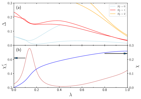
Figure S10: (a) The gap, $\Delta$, to the lowest lying $S^{z}_{T}=0,1,2$ states versus $\lambda$ for the $N=24Rh$ cluster. (b) The energy susceptibility, $\chi^{e}_{\lambda}$, and scalar chirality $\chi=\langle\mathbf{S}_{i}\cdot(\mathbf{S}_{j}\times\mathbf{S}_{k})\rangle$, versus $\lambda$ indicating a second order transition in the vicinity of $\lambda_{c}\approx 0.14$

It is expected Bauer et al. (2014) that the chiral spin liquid at $J_{\chi}=1,\ J_{3}=0$ is distinguishable from the phase of the nearest neighbor Heisenberg antiferromagnet on the kagomé lattice. To illustrate this we consider the following combined model extrapolating between the two limits:

$$H_{\lambda}=-\lambda J_{\chi}\sum_{\bigtriangleup,\bigtriangledown}\mathbf{S}_{i}\cdot\mathbf{S}_{j}\times\mathbf{S}_{k}+(1-\lambda)J\sum_{<i,j>}\mathbf{S}_{i}\cdot\mathbf{S}_{j}.$$ (S3.20)

Here, $J$ is the usual nearest neighbor (NN) coupling between sites on the kagomé lattice. We use the $N=24Rh$ unit cell to study the phase-diagram of $H_{\lambda}$ as $\lambda$ is varied between $\lambda=0$ (the pure NN HAF kagomé model) and $\lambda=1$ the purely chiral model. A convenient way of detecting quantum phase transitions is by analysing the ground-state energy susceptibility:

$$\chi^{e}_{\lambda}=-\frac{\partial^{2}e_{0}(\lambda)}{\partial\lambda^{2}},$$ (S3.21)

where $e_{0}$ is the ground-state energy per spin. It can be shown Albuquerque et al. (2010) that at a quantum critical point (QPT) $\chi^{e}_{\lambda}\sim L^{2/\nu-(d+z)}$, where $L$ is the linear size of the system. Hence, as long as $2/(d+z)>\nu$ we expect to see a divergence in $\chi_{\lambda}^{e}$ with $N,L$ at the QPT. Our results for the gap to the lowest lying states for $S^{z}_{T}=0,1,2$ are in Fig. S10(a) and for $\chi^{e}_{\lambda}$ in Fig. S10(b) along with the scalar chirality $\chi$. At $\lambda=0$ the spectrum is dominated by low-lying singlets with the gaps to $S_{T}^{z}=1,2$ states rapidly decreasing with $\lambda$. Close to $\lambda_{c}\sim 0.14$ a significant peak in $\chi^{e}_{\lambda}$ is visible consistent with a second order phase transition. At the same time $\chi$ increases from zero at $\lambda=0$ to $0.259$ for the CSL at $\lambda=1$ with the most rapid increase in the region around $\lambda_{c}\sim 0.14$. The saturation value of $\chi=0.259$ is slightly lower for the $N=24Rh$ cluster as compared to the value of $\chi=0.267$ ($J_{3}=0,h_{\mathrm{oct}}=0)$ for the $N=24$ cluster shown in Fig. S9(c), (d).

S3.6 Toy Model for Ferromagnetic bow-tie interaction

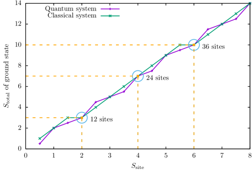
Figure S11: Total spin of the ground state vs the spin on each site of the triangle for both a quantum and a classical system with ${\mathcal{H}}={\mathcal{H}}_{\chi}+{\mathcal{H}}_{bt}$.

The ferromagnetic bow-tie Heisenberg interaction on the kagomé lattice for spin $S=1/2$, when added to a Chiral interaction, can be explained through a simple toy model. The idea is that at $J_{3}/J_{\chi}\rightarrow-\infty$, the kagomé lattice is broken up into three ferromagnetic square lattices. On these square lattices, each spin point to the same direction. Hence each square sub-lattice hosts a total spin state, $S_{\mathrm{square}}=N/6$, where $N$ is the total number of sites on the kagomé ($N/3$ being the number of sites on each square sub-lattice, multiplied by a spin $1/2$ on each site).

Now, when the chiral term is switched on, effectively, each triangle on the kagomé will act as if these large spins are interacting through a chiral like term. So we can find the ground state of the full problem by just solving a single triangle with a large spin, $S=S_{\mathrm{square}}$, present on each site. Doing so, we find the total spin of the ground state, which matches with the ED results on the $N=12,24,36$ site systems.

Furthermore, it can be seen that the resulting total spin of the ground state actually matches with the predicted classical value of spin. This is so as the classical ground state of the chiral plus a ferromagnetic bow-tie Heisenberg is just the XYZ order. For the XYZ order, the total classical spin length on each triangle is just $\sqrt{3}\cdot S$, and the quantum results match with this (upto taking a nearest integer value), as shown in fig.(S11).

References

- Balents (2010) Leon Balents, “Spin liquids in frustrated magnets,” Nature 464, 199–208 (2010).
- Grover et al. (2013) Tarun Grover, Yi Zhang, and Ashvin Vishwanath, “Entanglement entropy as a portal to the physics of quantum spin liquids,” New Journal of Physics 15, 025002 (2013).
- Savary and Balents (2016) Lucile Savary and Leon Balents, “Quantum spin liquids: a review,” Reports on Progress in Physics 80, 016502 (2016).
- Chamorro et al. (2021) Juan R. Chamorro, Tyrel M. McQueen, and Thao T. Tran, “Chemistry of quantum spin liquids,” Chemical Reviews 121, 2898–2934 (2021), pMID: 33156611, https://doi.org/10.1021/acs.chemrev.0c00641 .
- Kalmeyer and Laughlin (1987) V. Kalmeyer and R. B. Laughlin, “Equivalence of the resonating-valence-bond and fractional quantum hall states,” Phys. Rev. Lett. 59, 2095–2098 (1987).
- Schroeter et al. (2007) Darrell F. Schroeter, Eliot Kapit, Ronny Thomale, and Martin Greiter, “Spin hamiltonian for which the chiral spin liquid is the exact ground state,” Phys. Rev. Lett. 99, 097202 (2007).
- Yao and Kivelson (2007) Hong Yao and Steven A. Kivelson, “Exact chiral spin liquid with non-abelian anyons,” Phys. Rev. Lett. 99, 247203 (2007).
- Thomale et al. (2009) Ronny Thomale, Eliot Kapit, Darrell F. Schroeter, and Martin Greiter, “Parent hamiltonian for the chiral spin liquid,” Phys. Rev. B 80, 104406 (2009).
- Cincio and Vidal (2013) L. Cincio and G. Vidal, “Characterizing topological order by studying the ground states on an infinite cylinder,” Phys. Rev. Lett. 110, 067208 (2013).
- Bauer et al. (2014) B. Bauer, L. Cincio, B. P. Keller, M. Dolfi, G. Vidal, S. Trebst, and A. W. W. Ludwig, “Chiral spin liquid and emergent anyons in a kagome lattice mott insulator,” Nat Commun 5, 5137 (2014).
- He et al. (2014) Yin-Chen He, D. N. Sheng, and Yan Chen, “Chiral spin liquid in a frustrated anisotropic kagome heisenberg model,” Phys. Rev. Lett. 112, 137202 (2014).
- Gong et al. (2015) Shou-Shu Gong, Wei Zhu, Leon Balents, and D. N. Sheng, “Global phase diagram of competing ordered and quantum spin-liquid phases on the kagome lattice,” Phys. Rev. B 91, 075112 (2015).
- Wietek et al. (2015) Alexander Wietek, Antoine Sterdyniak, and Andreas M. Läuchli, “Nature of chiral spin liquids on the kagome lattice,” Phys. Rev. B 92, 125122 (2015).
- He et al. (2015) Yin-Chen He, Subhro Bhattacharjee, Frank Pollmann, and R. Moessner, “Kagome chiral spin liquid as a gauged symmetry protected topological phase,” Phys. Rev. Lett. 115, 267209 (2015).
- Wietek and Läuchli (2017) Alexander Wietek and Andreas M. Läuchli, “Chiral spin liquid and quantum criticality in extended heisenberg models on the triangular lattice,” Phys. Rev. B 95, 035141 (2017).
- Szasz et al. (2020) Aaron Szasz, Johannes Motruk, Michael P. Zaletel, and Joel E. Moore, “Chiral spin liquid phase of the triangular lattice hubbard model: A density matrix renormalization group study,” Phys. Rev. X 10, 021042 (2020).
- Hickey et al. (2016) Ciarán Hickey, Lukasz Cincio, Zlatko Papić, and Arun Paramekanti, “Haldane-hubbard mott insulator: From tetrahedral spin crystal to chiral spin liquid,” Phys. Rev. Lett. 116, 137202 (2016).
- Mekata (2003) Mamoru Mekata, “Kagome: The story of the basketweave lattice,” Physics Today 56, 12–13 (2003), https://doi.org/10.1063/1.1564329 .
- Hastings (2000) M. B. Hastings, “Dirac structure, rvb, and goldstone modes in the kagomé antiferromagnet,” Phys. Rev. B 63, 014413 (2000).
- Ran et al. (2007) Ying Ran, Michael Hermele, Patrick A. Lee, and Xiao-Gang Wen, “Projected-wave-function study of the spin- heisenberg model on the kagomé lattice,” Phys. Rev. Lett. 98, 117205 (2007).
- Iqbal et al. (2011) Yasir Iqbal, Federico Becca, and Didier Poilblanc, “Projected wave function study of spin liquids on the kagome lattice for the spin- quantum heisenberg antiferromagnet,” Phys. Rev. B 84, 020407 (2011).
- He et al. (2017) Yin-Chen He, Michael P. Zaletel, Masaki Oshikawa, and Frank Pollmann, “Signatures of dirac cones in a dmrg study of the kagome heisenberg model,” Phys. Rev. X 7, 031020 (2017).
- Iqbal et al. (2021) Yasir Iqbal, Francesco Ferrari, Aishwarya Chauhan, Alberto Parola, Didier Poilblanc, and Federico Becca, “Gutzwiller projected states for the heisenberg model on the kagome lattice: Achievements and pitfalls,” Phys. Rev. B 104, 144406 (2021).
- Messio et al. (2012) Laura Messio, Bernard Bernu, and Claire Lhuillier, “Kagome antiferromagnet: A chiral topological spin liquid?” Phys. Rev. Lett. 108, 207204 (2012).
- Helton et al. (2007) J. S. Helton, K. Matan, M. P. Shores, E. A. Nytko, B. M. Bartlett, Y. Yoshida, Y. Takano, A. Suslov, Y. Qiu, J.-H. Chung, D. G. Nocera, and Y. S. Lee, “Spin dynamics of the spin- kagome lattice antiferromagnet ,” Phys. Rev. Lett. 98, 107204 (2007).
- Khuntia et al. (2020) P. Khuntia, M. Velazquez, Q. Barthélemy, F. Bert, E. Kermarrec, A. Legros, B. Bernu, L. Messio, A. Zorko, and P. Mendels, “Gapless ground state in the archetypal quantum kagome antiferromagnet zncu3(oh)6cl2,” Nature Physics 16, 469–474 (2020).
- Smaha et al. (2020) Rebecca W. Smaha, Wei He, Jack Mingde Jiang, Jiajia Wen, Yi-Fan Jiang, John P. Sheckelton, Charles J. Titus, Suyin Grass Wang, Yu-Sheng Chen, Simon J. Teat, Adam A. Aczel, Yang Zhao, Guangyong Xu, Jeffrey W. Lynn, Hong-Chen Jiang, and Young S. Lee, “Materializing rival ground states in the barlowite family of kagome magnets: quantum spin liquid, spin ordered, and valence bond crystal states,” npj Quantum Materials 5, 23 (2020).
- Claassen et al. (2017) Martin Claassen, Hong-Chen Jiang, Brian Moritz, and Thomas P. Devereaux, “Dynamical time-reversal symmetry breaking and photo-induced chiral spin liquids in frustrated mott insulators,” Nature Communications 8, 1192 (2017).
- Zhang et al. (2021) Ya-Hui Zhang, D. N. Sheng, and Ashvin Vishwanath, “Su(4) chiral spin liquid, exciton supersolid, and electric detection in moiré bilayers,” Phys. Rev. Lett. 127, 247701 (2021).
- Jiang and Jiang (2020) Yi-Fan Jiang and Hong-Chen Jiang, “Topological superconductivity in the doped chiral spin liquid on the triangular lattice,” Phys. Rev. Lett. 125, 157002 (2020).
- Song et al. (2021) Xue-Yang Song, Ashvin Vishwanath, and Ya-Hui Zhang, “Doping the chiral spin liquid: Topological superconductor or chiral metal,” Phys. Rev. B 103, 165138 (2021).
- Semeghini et al. (2021) G. Semeghini, H. Levine, A. Keesling, S. Ebadi, T. T. Wang, D. Bluvstein, R. Verresen, H. Pichler, M. Kalinowski, R. Samajdar, A. Omran, S. Sachdev, A. Vishwanath, M. Greiner, V. Vuleti, and M. D. Lukin, “Probing topological spin liquids on a programmable quantum simulator,” Science 374, 1242–1247 (2021), https://www.science.org/doi/pdf/10.1126/science.abi8794 .
- Nagaosa and Tokura (2013) Naoto Nagaosa and Yoshinori Tokura, “Topological properties and dynamics of magnetic skyrmions,” Nature Nanotechnology 8, 899–911 (2013).
- Fert et al. (2017) Albert Fert, Nicolas Reyren, and Vincent Cros, “Magnetic skyrmions: advances in physics and potential applications,” Nature Reviews Materials 2, 17031 (2017).
- Kurumaji et al. (2019) Takashi Kurumaji, Taro Nakajima, Max Hirschberger, Akiko Kikkawa, Yuichi Yamasaki, Hajime Sagayama, Hironori Nakao, Yasujiro Taguchi, Taka hisa Arima, and Yoshinori Tokura, “Skyrmion lattice with a giant topological hall effect in a frustrated triangular-lattice magnet,” Science 365, 914–918 (2019), https://www.science.org/doi/pdf/10.1126/science.aau0968 .
- Hirschberger et al. (2019) Max Hirschberger, Taro Nakajima, Shang Gao, Licong Peng, Akiko Kikkawa, Takashi Kurumaji, Markus Kriener, Yuichi Yamasaki, Hajime Sagayama, Hironori Nakao, Kazuki Ohishi, Kazuhisa Kakurai, Yasujiro Taguchi, Xiuzhen Yu, Taka-hisa Arima, and Yoshinori Tokura, “Skyrmion phase and competing magnetic orders on a breathing kagomélattice,” Nature Communications 10, 5831 (2019).
- Hayami et al. (2021) Satoru Hayami, Tsuyoshi Okubo, and Yukitoshi Motome, “Phase shift in skyrmion crystals,” Nature Communications 12, 6927 (2021).
- Wang et al. (2022) Weiwei Wang, Dongsheng Song, Wensen Wei, Pengfei Nan, Shilei Zhang, Binghui Ge, Mingliang Tian, Jiadong Zang, and Haifeng Du, “Electrical manipulation of skyrmions in a chiral magnet,” Nature Communications 13, 1593 (2022).
- Ortiz et al. (2019) Brenden R. Ortiz, Lidia C. Gomes, Jennifer R. Morey, Michal Winiarski, Mitchell Bordelon, John S. Mangum, Iain W. H. Oswald, Jose A. Rodriguez-Rivera, James R. Neilson, Stephen D. Wilson, Elif Ertekin, Tyrel M. McQueen, and Eric S. Toberer, “New kagome prototype materials: discovery of kv3sb5,rbv3sb5, and csv3sb5,” Phys. Rev. Materials 3, 094407 (2019).
- Zhao et al. (2021) He Zhao, Hong Li, Brenden R. Ortiz, Samuel M. L. Teicher, Takamori Park, Mengxing Ye, Ziqiang Wang, Leon Balents, Stephen D. Wilson, and Ilija Zeljkovic, “Cascade of correlated electron states in the kagome superconductor csv3sb5,” Nature 599, 216–221 (2021).
- Jiang et al. (2021) Yu-Xiao Jiang, Jia-Xin Yin, M. Michael Denner, Nana Shumiya, Brenden R. Ortiz, Gang Xu, Zurab Guguchia, Junyi He, Md Shafayat Hossain, Xiaoxiong Liu, Jacob Ruff, Linus Kautzsch, Songtian S. Zhang, Guoqing Chang, Ilya Belopolski, Qi Zhang, Tyler A. Cochran, Daniel Multer, Maksim Litskevich, Zi-Jia Cheng, Xian P. Yang, Ziqiang Wang, Ronny Thomale, Titus Neupert, Stephen D. Wilson, and M. Zahid Hasan, “Unconventional chiral charge order in kagome superconductor kv3sb5,” Nature Materials 20, 1353–1357 (2021).
- Khasanov et al. (2022) Rustem Khasanov, Debarchan Das, Ritu Gupta, Charles Mielke, Matthias Elender, Qiangwei Yin, Zhijun Tu, Chunsheng Gong, Hechang Lei, Ethan Ritz, Rafael M. Fernandes, Turan Birol, Zurab Guguchia, and Hubertus Luetkens, “Charge order breaks time-reversal symmetry in csv3sb5,” (2022).
- Neupert et al. (2022) Titus Neupert, M. Michael Denner, Jia-Xin Yin, Ronny Thomale, and M. Zahid Hasan, “Charge order and superconductivity in kagome materials,” Nature Physics 18, 137–143 (2022).
- Teng et al. (2022) Xiaokun Teng, Lebing Chen, Feng Ye, Elliott Rosenberg, Zhaoyu Liu, Jia-Xin Yin, Yu-Xiao Jiang, Ji Seop Oh, M. Zahid Hasan, Kelly J. Neubauer, Bin Gao, Yaofeng Xie, Makoto Hashimoto, Donghui Lu, Chris Jozwiak, Aaron Bostwick, Eli Rotenberg, Robert J. Birgeneau, Jiun-Haw Chu, Ming Yi, and Pengcheng Dai, “Discovery of charge density wave in a correlated kagome lattice antiferromagnet,” (2022).
- Kivelson et al. (1987) Steven Kivelson, C. Kallin, Daniel P. Arovas, and J. Robert Schrieffer, “Cooperative ring exchange and the fractional quantum hall effect,” Phys. Rev. B 36, 1620–1646 (1987).
- Chubukov et al. (1994) Andrey V. Chubukov, Subir Sachdev, and T. Senthil, “Quantum phase transitions in frustrated quantum antiferromagnets,” Nuclear Physics B 426, 601–643 (1994).
- Wen et al. (1989) X. G. Wen, Frank Wilczek, and A. Zee, “Chiral spin states and superconductivity,” Phys. Rev. B 39, 11413–11423 (1989).
- Fradkin and Schaposnik (1991) Eduardo Fradkin and Fidel A. Schaposnik, “Chern-simons gauge theories, confinement, and the chiral spin liquid,” Phys. Rev. Lett. 66, 276–279 (1991).
- Zhang and Li (2021) Qiu Zhang and Tao Li, “Bosonic resonating valence bond theory of the possible chiral spin-liquid state in the triangular-lattice hubbard model,” Phys. Rev. B 104, 075103 (2021).
- Pitts et al. (2021) Jackson Pitts, Finn Lasse Buessen, Roderich Moessner, Simon Trebst, and Kirill Shtengel, “Order by disorder in classical kagome antiferromagnets with chiral interactions,” (2021), arXiv:2110.11427 [cond-mat.str-el] .
- Messio et al. (2011) L. Messio, C. Lhuillier, and G. Misguich, “Lattice symmetries and regular magnetic orders in classical frustrated antiferromagnets,” Phys. Rev. B 83, 184401 (2011).
- Watanabe (2020) Haruki Watanabe, “Counting rules of nambu goldstone modes,” Annual Review of Condensed Matter Physics 11, 169–187 (2020), https://doi.org/10.1146/annurev-conmatphys-031119-050644 .
- (53) Supplementary Information contains details of (i) Linear spin wave theory including extrapolation of correlations to the thermodynamic limit, (ii) Parton mean field theory, (iii) Exact Diagonalization calculations with additional results.
- Marston and Zeng (1991) J. B. Marston and C. Zeng, “Spin-peierls and spin-liquid phases of kagomé quantum antiferromagnets,” Journal of Applied Physics 69, 5962–5964 (1991), https://doi.org/10.1063/1.347830 .
- Hu et al. (2015) Wen-Jun Hu, Wei Zhu, Yi Zhang, Shoushu Gong, Federico Becca, and D. N. Sheng, “Variational monte carlo study of a chiral spin liquid in the extended heisenberg model on the kagome lattice,” Phys. Rev. B 91, 041124 (2015).
- Leung and Elser (1993) P. W. Leung and Veit Elser, “Numerical studies of a 36-site kagome antiferromagnet,” Phys. Rev. B 47, 5459–5462 (1993).
- Waldtmann et al. (1998) C. Waldtmann, H. U. Everts, B. Bernu, C. Lhuillier, P. Sindzingre, P. Lecheminant, and L. Pierre, “First excitations of the spin 1/2 heisenberg antiferromagnet on the kagomélattice,” The European Physical Journal B - Condensed Matter and Complex Systems 2, 501–507 (1998).
- Läuchli et al. (2019) Andreas M. Läuchli, Julien Sudan, and Roderich Moessner, “ kagome heisenberg antiferromagnet revisited,” Phys. Rev. B 100, 155142 (2019).
- Läuchli et al. (2011) Andreas M. Läuchli, Julien Sudan, and Erik S. Sørensen, “Ground-state energy and spin gap of spin- kagomé-heisenberg antiferromagnetic clusters: Large-scale exact diagonalization results,” Phys. Rev. B 83, 212401 (2011).
- Hickey et al. (2017) Ciarán Hickey, Lukasz Cincio, Zlatko Papić, and Arun Paramekanti, “Emergence of chiral spin liquids via quantum melting of noncoplanar magnetic orders,” Phys. Rev. B 96, 115115 (2017).
- Oliviero et al. (2021) Fabrizio Oliviero, João Augusto Sobral, Eric C. Andrade, and Rodrigo G. Pereira, “Noncoplanar magnetic orders and gapless chiral spin liquid in the -- model on the kagome lattice,” (2021).
- Tóth and Lake (2015) Sándor Tóth and Bella Lake, “Linear spin wave theory for single-q incommensurate magnetic structures.” Journal of physics. Condensed matter : an Institute of Physics journal 27 16, 166002 (2015).
- Colpa (1978) J. H. P. Colpa, “Diagonalization of the quadratic boson hamiltonian,” Physica A Statistical Mechanics and its Applications 93, 327–353 (1978).
- Fukui et al. (2005) Takahiro Fukui, Yasuhiro Hatsugai, and Hiroshi Suzuki, “Chern numbers in a discretized Brillouin zone: Efficient method to compute (spin) Hall conductances,” J. Phys. Soc. Jap. 74, 1674–1677 (2005), arXiv:cond-mat/0503172 .
- Albuquerque et al. (2010) A. Fabricio Albuquerque, Fabien Alet, Clément Sire, and Sylvain Capponi, “Quantum critical scaling of fidelity susceptibility,” Phys. Rev. B 81, 064418 (2010).