galstreams: A Library of Milky Way Stellar Stream Footprints and Tracks

Cecilia Mateu,¹
¹Departamento de Astronomía, Facultad de Ciencias, Universidad de la República, Iguá 4225, 14000, Montevideo, Uruguay
E-mail: cmateu@fcien.edu.uy

(Accepted XXX. Received YYY; in original form ZZZ)

Abstract

Nearly a hundred stellar streams have been found to date around the Milky Way and the number keeps growing at an ever faster pace. Here we present the galstreams library, a compendium of angular position, distance, proper motion and radial velocity track data for nearly a hundred (95) Galactic stellar streams. The information published in the literature has been collated and homogenised in a consistent format and used to provide a set of features uniformly computed throughout the library: e.g. stream length, end points, mean pole, stream’s coordinate frame, polygon footprint, and pole and angular momentum tracks. We also use the information compiled to analyse the distribution of several observables across the library and to assess where the main deficiencies are found in the characterisation of individual stellar streams, as a resource for future follow-up efforts. The library is intended to facilitate keeping track of new discoveries and to encourage the use of automated methods to characterise and study the ensemble of known stellar streams by serving as a starting point. The galstreams library is publicly available as a Python package and served at the galstreams GitHub repository.

keywords:

software: public release – Galaxy: structure – Galaxy: halo – Astronomical databases: catalogues

^†^†pubyear: 2022^†^†pagerange: galstreams: A Library of Milky Way Stellar Stream Footprints and Tracks–A

1 Introduction

The field of stellar streams is currently in a golden era. It has increasingly grown and all but exploded in the last decade (see e.g. Grillmair & Carlin, 2016; Helmi, 2020), thanks to deep wide-area photometric surveys (SDSS, PS-1, DES Grillmair, 2009; Bernard et al., 2016; Grillmair, 2017b; Shipp et al., 2018) and, more recently, to the amazing possibilities opened by the all-sky astrometric information provided by the Gaia mission since its Second Data Release (DR2 Gaia Collaboration et al., 2018; Malhan & Ibata, 2018; Ibata et al., 2021). The availability of widespread kinematic information is having a tremendous impact. From the observational standpoint, enabling a large number of new stellar stream discoveries (see Table 1 for a complete list), revealing relationships between streams far apart (e.g. Orphan/Chenab, ATLAS/Aliqa Uma Koposov et al., 2019; Li et al., 2021), linking known streams (Fimbulthul, Gjöll, Fjörm) to their globular cluster progenitors ( $\omega$ Cen, NGC 3201, M68 Ibata et al., 2019a, 2021; Palau & Miralda-Escudé, 2019, 2021); while at the same time revealing intriguing features like gaps, "spurs", a "cocoon" and a "blob" in GD-1 some potentially due to dark matter subhalos (Price-Whelan & Bonaca, 2018; Bonaca et al., 2019a; Malhan et al., 2019; de Boer et al., 2020), and (at first) unexpected features like the misalignment of velocities with stream tracks found first in the Orphan-Chenab stream (Koposov et al., 2019) and later observed in several of the Dark Energy Survey streams (Shipp et al., 2018), now thought to be perturbations caused by a recent close passage of the Large Magellanic Cloud (Erkal et al., 2019; Shipp et al., 2020). At the same time, from the theoretical standpoint, it is now making it feasible to advance some of the astrophysical questions that have long motivated interest in stellar streams, like reconstructing the assembly history of the Milky Way (e.g. Naidu et al., 2020; Bonaca et al., 2021; Malhan et al., 2022), inferring the shape and mass of its dark matter halo (Malhan & Ibata, 2019; Reino et al., 2021; Vasiliev et al., 2021; Cautun et al., 2020) and constraining properties of dark matter subhaloes (Erkal et al., 2017; Bonaca et al., 2019a; Bonaca et al., 2020; Banik et al., 2021; Malhan et al., 2021a; Gialluca et al., 2021).

In the past six years alone, the number of new streams reported in the literature increased almost five-fold, going from $\sim$ 20 reported in Grillmair & Carlin (2016) to nearly a hundred compiled in this work (see Figure 1). This rate of discovery is not yet showing signs of reaching saturation and is even likely to increase as deep photometry from the Legacy Survey of Space and Time (LSST at the Vera Rubin Observatory, Ivezić et al., 2019) will allow probing fainter structures and farther reaches of the Galactic halo. Such a rapid growth makes a compilation as challenging as it makes it necessary. Challenging, not only because of the fast pace, but because the growth of the field has been, and continues to be, entirely organic. Because of their very nature as extended structures, the reporting of stellar stream properties \textcolorblack(position in the sky, angular width, kinematics, etc.) in the literature has been -to put it mildly- heterogeneous. Necessary, because systematic studies of Galactic stellar streams as a system require a homogeneous compendium as a starting point.

In Mateu et al. (2018) we published galstreams, a first compilation of tidal stream footprints implemented as a Python library. It was based on the compilation by Grillmair & Carlin (2016, their Tables 4.1 and 4.2) and expanded the information available from approximate RA $/$ Dec or $l/b$ regions to extended footprints. Its initial aim was to keep track of known stellar streams and overdensities and to homogenise the available information so that it could be parsed in an automated way and would facilitate identifying whether a stream is indeed a new discovery or which streams are present in a given patch of the sky. In that version (v0.1), pre-Gaia DR2, the library contained only celestial positions and distance information to represent the area covered by a stream in the sky. Since then, many studies have used Gaia DR2 and EDR3 (Gaia Collaboration et al., 2018, 2021) to find and characterise the proper motion signature of many stellar streams, complemented with radial velocity data from existing and new dedicated follow-ups for a several of them (e.g. Ibata et al., 2021; Li et al., 2022). Hence, a much more rich compilation including kinematics is now possible for a large number of stellar streams.

Our goal in this paper and with the new version (v1) of the galstreams library is to collate the available information to provide \textcolorblacka homogeneous framework with celestial, distance, proper motion and radial velocity track¹¹1\textcolorblackgalstreams does not provide data for individual member stars for any stream. \textcolorblackinformation available in the literature for the tidal streams found in the Milky Way. Such a compilation will make it easier to identify when a discovery is indeed a new structure and to find connections between structures scattered across the sky, and will be an essential starting point for future automated systematic searches for new members of known streams. It is also intended as a resource for the community to identify where efforts can be directed to collect missing or insufficient information for the less studied streams, and avoid duplicating efforts when planning new observations.

The structure of the paper is as follows: In Sec. 2 we present an overview of the information compiled in the library and discuss improvements with respect to the previous version of galstreams. In Sec. 3 we present the general procedures used to implement the tracks for the streams found in the literature (Sec. 3.1) and describe for each one the specific information used to implement it (Sec. 3.2). In Sec. 3.3 we discuss structures that are not included in the library. In Sec. 4 we compare tracks for streams with multiple instances available and discuss the criteria used to decide the track selected as the default in each case. In Sec. 5 we use the library to discuss properties of the system of stellar streams as a whole and conclude with a summary in Sec. 6.

2 The galstreams library

Refer to caption — Figure 1: Mollweide projection map in Galactic coordinates of the celestial tracks for the 95 stellar streams implemented in the library. The position of the Large and Small Magellanic Clouds (LMC, SMC) is also shown for reference.

The galstreams library can be viewed as a compilation of stream’s meta-data: it includes information needed to locate a given tidal stream in the sky (v0.1) and its signature in kinematics (v1). \textcolorblackThis information is provided as a track in up to 6D, each dimension being a one dimensional function describing each component (e.g. distance or proper motion in a given direction) as a function of an angle in the sky. As will be described in Sec. 3.1, tracks are not orbital fits, they are empirical fits to observed data, obtained either as interpolations from reported knots or reference points or as polynomial fits to members reported in the literature.

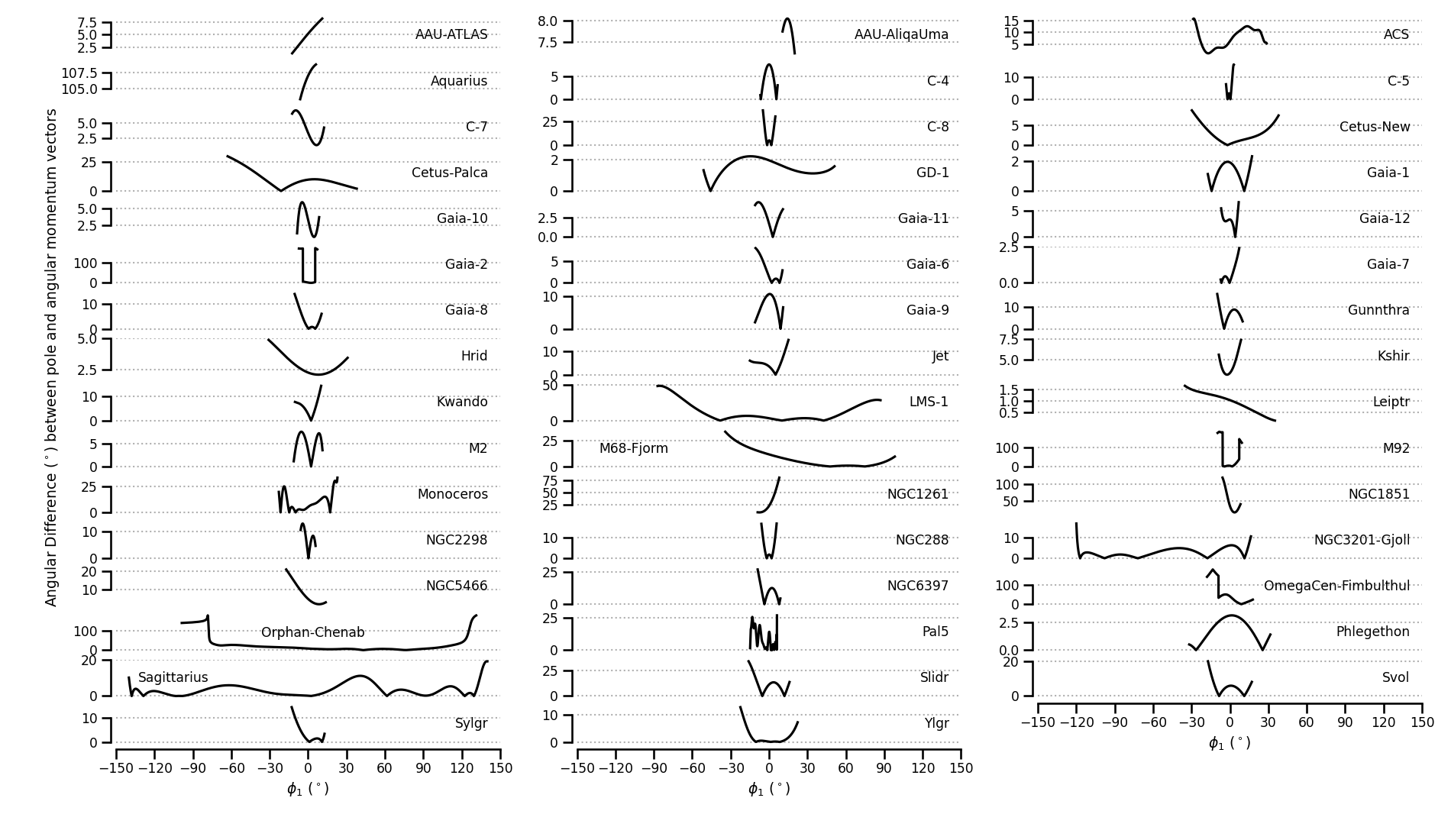
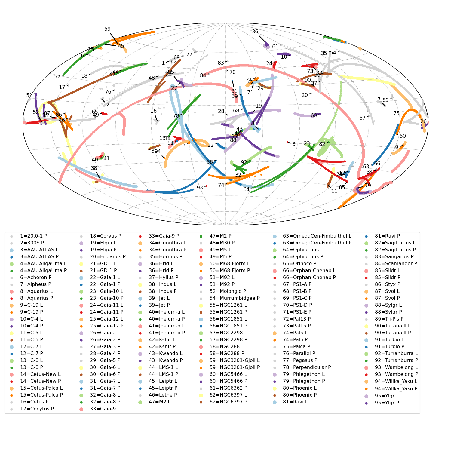
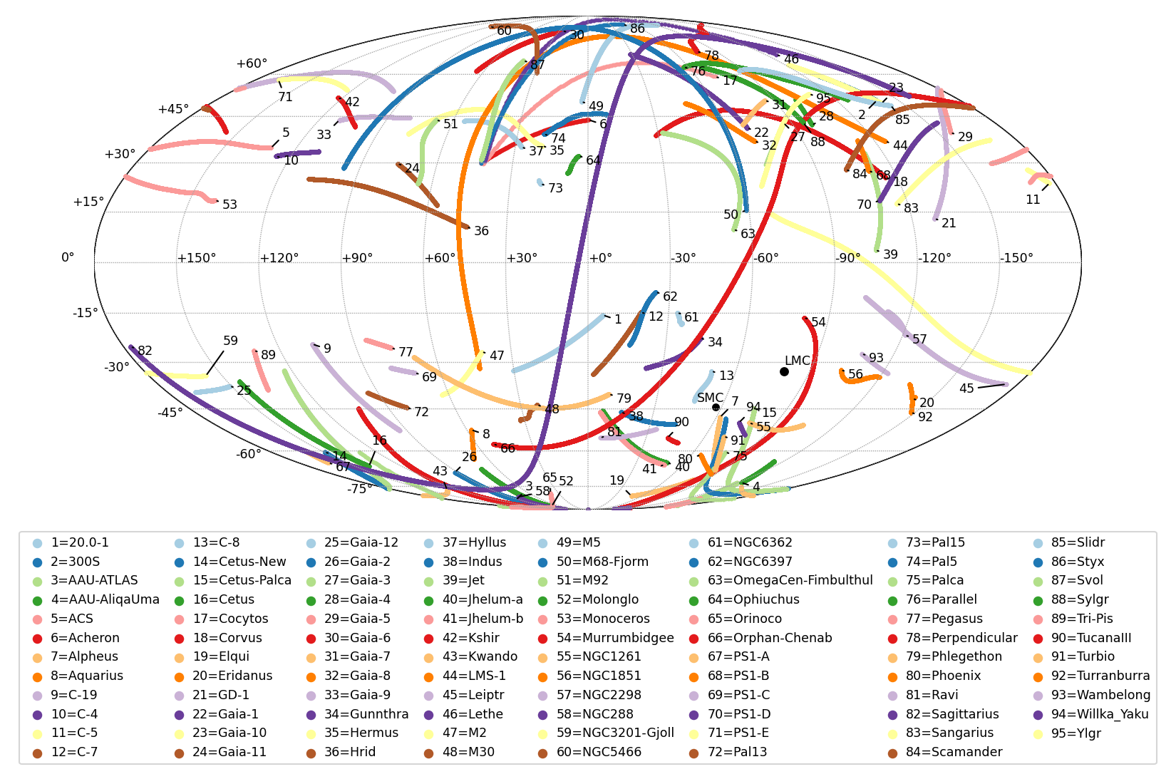
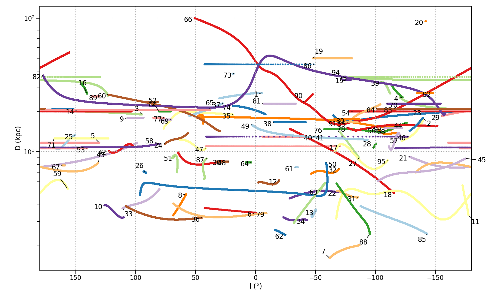
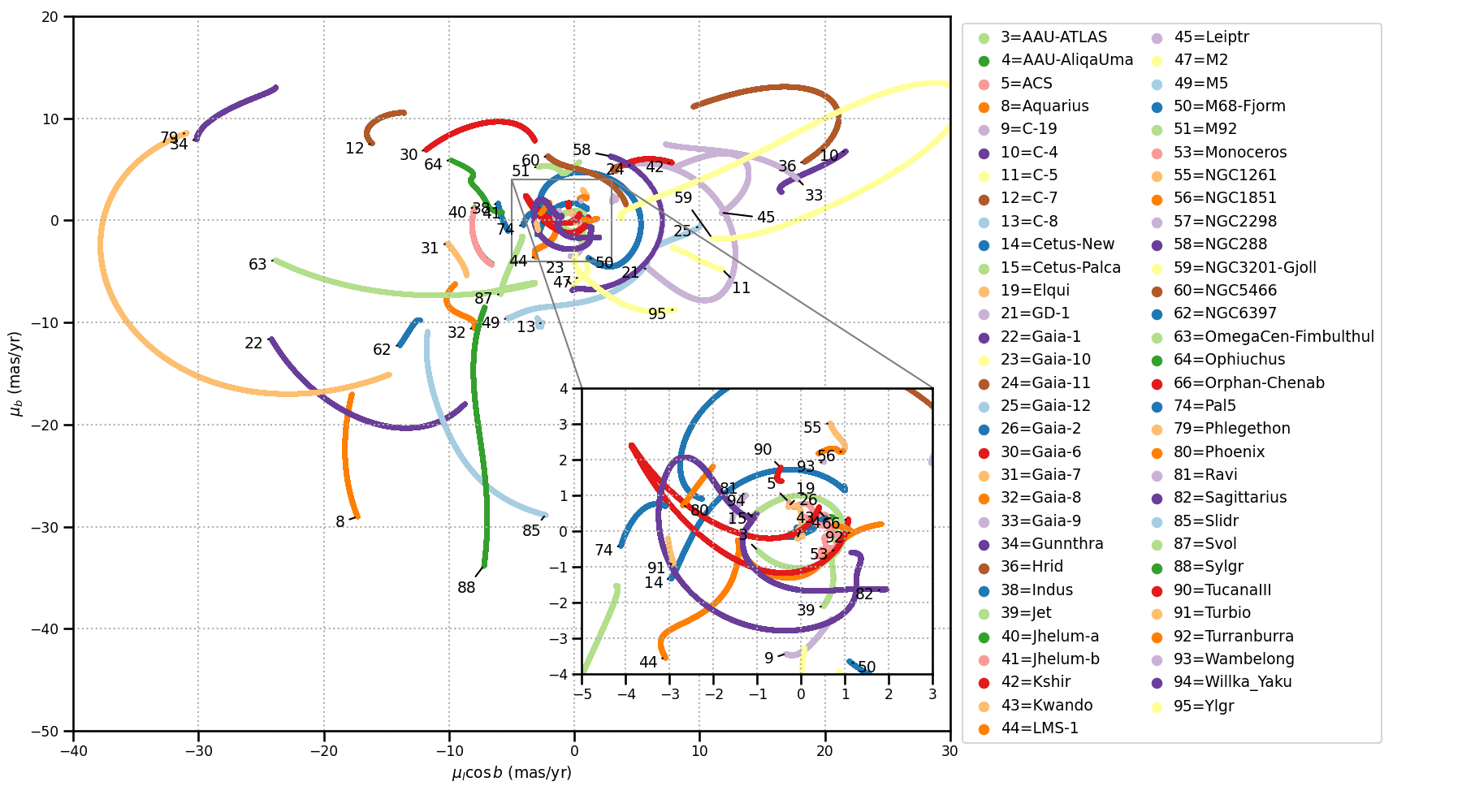
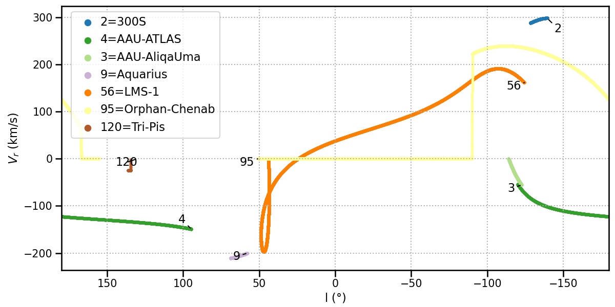
The library is implemented in Python, based on astropy, and served at the galstreams public repository on GitHub²²2Available at https://github.com/cmateu/galstreams. Figure 1 shows a map of the celestial tracks for the 95 unique stellar streams (i.e. no repetitions), out of the total of 126 tracks implemented in the galstreams library \textcolorblackbased on information published from different sources in the literature, in which multiple tracks are available for same stellar stream in several instances (see discussion in Sec. 4). \textcolorblackFigure 2 shows the distance tracks as a function of Galactic longitude for the 95 stellar streams in the library, Figure 3 the proper motion in Galactic latitude versus the proper motion in Galactic longitude for the 61 streams with proper motion information in the library, and Figure 4 the radial velocity as a function of Galactic longitude for the $7$ tracks with this information available in the library. Table 1 summarises the information available for all the stream tracks implemented in the library following the procedure described in Sec. 3.1.

The main features of the library in its current version are:

•

Tracks \textcolorblackin up to 6D: sky, distance, proper motion and radial velocity tracks for each stream
•

Stream’s (heliocentric) coordinate frame realised as an astropy reference frame
•

Polygon Footprints
•

End-points and mid-point celestial coordinates
•

Pole (at mid point) and pole tracks in the heliocentric and Galactocentric frames for all tracks in the library
•

Angular momentum track in the heliocentric reference frame at rest with respect to the Galactic centre \textcolorblack(for tracks with proper motion data available)
•

Summary object with attributes for the full library: Uniformly reported end points and mid-point, heliocentric and Galactocentric mid-pole, track angular length, track and discovery references and an information flag denoting which of the 6D attributes (sky, distance, proper motions and radial velocity) are available in the track object

Although track information is derived from individual stream members when available in the literature, galstreams does not supply information for individual members. The 6D tracks and polygon footprints provided should, however, provide a useful tool to conduct automated systematic searches for individual stream members.

2.1 Improvements and changes with respect to galstreams v0.1

In its original version (v0.1) the main piece of information provided by galstreams was each stream’s Footprint created as a random realisation with uniform area coverage in the sky, \textcolorblackincluding either mean distance information or distance as a function of position along the footprint, for the relatively few streams where this information was available. An extension was later added to calculate end points and poles from these random realisations, as a means of providing a quick-and-dirty way of realising each stream’s coordinate frame, mainly for plotting purposes.

In this new version, the main feature of the library is to provide each stream’s track in up to 6D: the sky, distance, proper motions and radial velocity tracks are reported for streams with data available in the literature. Because of the potential use in qualitative plots, a method to produce random realisations of the tracks is provided.

The representation as a celestial track, rather than a randomly populated footprint, is more suited to the nature of the streams we want to represent and allows for a better record keeping of useful stream attributes and their dependencies, such as correlations of distance, radial velocity or proper motion with celestial coordinates. In future versions, other attributes could also be supported in this representation, e.g. width and error tracks or other attributes relating to the stellar population like age and metallicity. New Polygon Footprints, also provided, are constructed based on the tracks. These provide an easy way to select a catalogue’s points inside a stream’s footprint and to create a similar off-stream selection area for background subtraction.

The stream’s track is stored as an astropy SkyCoord object and, as of this version, distance information is required for a stream to be included in the library. This way the track has all coordinate transformation capabilities available in astropy and making the distance a mandatory attribute allows for the track to be easily transformed into any non-heliocentric reference frame, in particular, the Local or Galactocentric Standards of Rest (LSR and GSR, respectively). Although a distance estimate was not mandatory in the previous version, in practice all streams in galstreams v0.1 had it, except for the WG1-4 streams from Agnello (2017). Since there is no further available information for these candidates (proper motions, radial velocity or any information about the stellar population), we have decided not to include WG1-4 in the library and to make a distance estimate (however rough) a mandatory attribute.

Up to the previous version we had also included footprint realisations for the cloud-like features compiled in Table 4.2 of Grillmair & Carlin (2016): Tri-And I and II, Hercules-Aquila and the Virgo and Pisces Overdensities (see also Sec. 3.3, about the Virgo Stellar Stream, VSS). We are aiming now at providing more descriptive information that is specific to streams and not meaningful for clouds, so we have decided not to include these or other diffuse structures in galstreams. The original motivation to include them was for the user to be aware of any known overdensities in a given region of the sky. The discovery of localised overdensities does not seem to have proliferated since the publication of Gaia DR2; in contrast, major accretion events have been identified, such as Gaia-Enceladus-Sausage or Gaia-Sausage Merger (Belokurov et al., 2018; Helmi et al., 2018), Thamnos (Koppelman et al., 2019), Sequoia (Myeong et al., 2019); Arjuna, Sequoia and I’itoi (Naidu et al., 2020); Heracles (Horta et al., 2021) and Pontus (Malhan, 2022). These features are not localised, spanning vast regions (if not all) of the celestial sphere. Hence, we have decided to keep the library focused only on stream-like overdensities and not to include any of these structures (see Sec. 3.3 for more details on excluded structures).

The library has been updated to include newly discovered streams (2020–2022), as well as streams published previously in the literature but missing in the first version (e.g. 300S, Aquarius, Parallel and Perpendicular). To the best of our knowledge, galstreams is up to date as of mid-March 2022 and will be kept updated and documented in the GitHub repository, following the format and procedures described here.

3 Streams’ data and track realisations

3.1 Procedure

The data for stellar streams and the format in which it is reported in the literature is very heterogeneous: it can be comprised of anything from a pole or end-point coordinates, a list of stream members, polynomial equations or spline knots with an arbitrary celestial coordinate acting as free parameter, to a stream track marked or tidal tails shown in a sky projection plot. The initial data for any given stream inevitably needs to be collected and parsed manually into a data set that galstreams can then handle uniformly and implement as a track with other associated attributes computed automatically for each one.

The first step after the initial data collection is to create a set of points to represent the track. Overall, the data available for each stream can be classified into one of these categories: (i) End points, (ii) Pole, mid point and length and (iii) Custom. The first two are closely related and easy to implement automatically. In the third case, which comprises the majority of streams in the literature, typically a polynomial interpolation or fit will be used to produce a track from the collected data (described for each stream in detail in Sec. 3.2). In this case, because of each stream’s different orientation in space, the celestial coordinate that can act as the independent variable will be different. However, the natural reference frame to realise each stream’s track automatically is its own frame, i.e. that in which the stream lies approximately in the equator and in it, the natural independent variable is the longitude or azimuthal variable usually named $\phi_{1}$ . In most cases, this frame is not known a priori and needs to be inferred from the data itself. To homogenise this starting data set from which the track attributes are computed, galstreams uses the following internal procedure:

•

For each stream a set of densely populated reference points or knots along the track is produced. We describe what data is available and how this is done, for each individual stream in Sec. 3.2. The set of knots created for each stream is dense enough so that simple linear interpolation can be performed later to evaluate the track at any given point and the stability of the interpolation is ensured. This set of knots will define the stream’s track.
•

In case i), when end point’s coordinates are provided, the initial set of points is realised as uniformly spaced points along the ?(shortest) great circle arc connecting them.
•

Similarly, in case ii), when the pole, mid point and length are provided, the end points are computed and an initial set of points is realised along the great circle as described in the previous point.
•
When an initial track or set of candidate points is reported and there is no existing information either on the end-points, pole or directly the reference frame’s rotation matrix, this is guessed automatically based on the data collected from the literature, as follows:
- –
  
  The geometric average of the first and last point is used as an initial guess for the mid-point and pole. This guess is provisional as this average is, in general, not along the stream track and –unless the input is already a track– these points are not necessarily representative of the track’s end points. An initial stream frame is realised with these parameters and the points rotated to this reference frame. In this initial reference frame $\phi_{1}$ can be used as an independent variable and the knots, defined as a set of points uniformly spaced in $\phi_{1}$ , will lie reasonably close to the frame’s equator ( $\phi_{2}\sim 0\degr$ ).
- –
  
  In this initial frame, the new reference point’s coordinates $(\phi_{1},\phi_{2})$ are found by interpolating the knots’ $\phi_{2}$ at the mean $\phi_{1}$ . This point will lie along the track by construction and is a reasonable approximation of a mid-point.
- –
  
  Next, two points near the reference point (within $0\aas@@fstack{\circ}5$ ) are used to compute a new pole. The stream’s reference frame is now computed using the new mid-point and pole. This reference frame ensures the mid-point is at the origin and the track stays close to $\phi_{2}\sim 0\degr$ around it.
•

The literature data points are transformed to the stream’s reference frame and are either interpolated (when an equation or knots are provided) or fitted with a polynomial (when individual stream members are) to reduce the points to a track. Once the interpolator or polynomial fitting object is built in the stream’s frame, in each of the available (up to 6D) coordinates the track knots to be stored are realised by populating the track between the identified end points with an arbitrary uniform spacing of $0\aas@@fstack{\circ}01$ . This resolution was found to be high enough so that in any later step linear interpolation in the track is sufficient and stable. The stream’s knots and reference frame are stored internally.
•
\textcolor
black Heliocentric and galactocentric pole tracks are provided for all streams in the library, as are the mid-pole (pole coordinates at the stream’s mid-point) in both reference frames. In a given frame, the pole track is computed as the vector product between the position vectors of each pair of consecutive points along a stream. This provides a normal or pole vector that may change along the track if the stream is not perfectly planar. Because of the difference in point of view between a heliocentric and Galactocentric observer, pole tracks will depend on the reference frame, hence, pole tracks are reported for both reference frames.
•
\textcolor
blackAngular momentum tracks in a heliocentric reference frame at rest with the GSR are provided for all streams with proper motion information available in the library (see discussion in Sec 5.5). This angular momentum is computed as $\mathbf{L_{\mathrm{hel}}}=\mathbf{r_{\mathrm{hel}}}\times\mathbf{v}_{\mathrm{GSR}}$ , where $\mathbf{r}_{\mathrm{hel}}$ is the heliocentric position and $\mathbf{v}_{\mathrm{GSR}}$ is the velocity with respect to the GSR. It is convenient to use this reference frame because the radial velocity of the stream has no contribution to the angular momentum and this component is only available for a small number of tracks in the library ( $7$ out of $126$ ).

The library’s policy is to compile data and summary statistics computed from a homogeneous set of direct observables. In some papers predicted proper motion or radial velocity tracks are reported, these are not included in the library. Also, solar-reflex corrected proper motion tracks and GSR radial velocities are commonly reported in the literature. Since these are dependent on the position and velocity assumed for the Sun and the LSR, we choose to report instead the observed heliocentric proper motions and radial velocity tracks, i.e. without having subtracted the solar reflex motion. The solar reflex correction can be easily applied by the user consistently across the library with their preferred solar and LSR parameters³³3e.g. in Python using the reflex_correct method in gala (Price-Whelan, 2017).

For now, the purpose of galstreams is to allow comparison of new features with know ones and to allow visualising the system of stellar streams in the Galaxy as a whole. This is, of course, an incomplete view. Information about the stellar population, e.g. age, metallicity or $\mathrm{[\alpha/Fe]}$ , is not included. No judgement is made as to the confidence or robustness of the detection of the streams listed in the library, some having much more available information than others thanks to dedicated follow-up studies. The positional and kinematic information and data flags provided are intended to serve as a tool for users to form their own criteria as to which streams they consider as better characterised or feel more confident in. Therefore, user discretion is advised.

3.2 Individual stream track implementations

Table 1 presents a summary for the 126 tracks implemented from different sources for the 95 (unique) streams currently available in galstreams. \textcolorblackHow multiple tracks for a given stream are dealt with and the criteria on which this is decided is discussed for each case with multiple tracks in Sec 4. \textcolorblackThe naming convention followed for streams with multiple tracks that have different names in the literature, but have been robustly identified as being part of the same stream (e.g. Orphan and Chenab), is that each track is labelled with the original name used by each author (Orphan-K19 and Chenab-S19 tracks) and all are ascribed to the same stream with a compound name (Orphan-Chenab stream). Depending on the data available for each stream its 6D track was implemented following one of the three methods described in Sec. 3.1: (i) Streams realised as great circle arcs from reported end points, (ii) Streams realised as great circle arcs defined by their reported poles and (iii) Streams realised from custom data. \textcolorblackThe method used to implement the track is indicated in Table 1 in the Imp (implementation) column for each of the categories described in the previous section (ep=end points, po=pole, st=individual stars or knots). The InfoFlags column indicates which of the 6D data is available for each stream and keeps track of any assumptions made in each track implementation: the first character is 0 if the stream is assumed to be a great circle and 1 if not; the second, third and fourth characters indicate whether distance, proper motions and radial velocity tracks are available (1) or not (0). Whenever the distance, proper motion or radial velocity measurements are available but there is a caveat, it is indicated with ‘2’ (see e.g. M5-G19 and Ravi). In these cases, see the documentation for details on each particular stream. The ‘On’ column indicates which of the tracks is set as the default for a given stream. The stream’s length along the track, equatorial coordinates and distances for the end points are also reported in the table. Finally, the TRefs and DRefs columns indicate with a unique code the references for the track implementation and the stream’s discovery, respectively. The reference corresponding to each code is found in Table 3.

In what follows we briefly describe the specific information used to implement each attribute (position, distance, proper motion, radial velocity) of a stream’s track and its individual provenance. \textcolorblackAs will become apparent, for many streams the data needed to implement the tracks was only available from figures, not tables or quantitative data provided in the article’s text. In these cases, the data has been read-off the relevant plots cited using the WebPlotDigitizer tool. ⁴⁴4Available at https://apps.automeris.io/wpd/

20.0-1-M18

The celestial track was implemented as the great circle arc (of minimum length) with galactocentric pole, mid-point coordinates and length as reported by Mateu et al. (2018). The mean galactocentric distance reported by the authors was adopted for the full track. The coordinates were transformed back to the heliocentric frame assuming $R_{\odot}=-8.5$ kpc, as adopted by the authors.

300S-F18

The celestial, distance and radial velocity tracks were read-off the fit shown by Fu et al. (2018) in their Figure 10. Note that the stream members observed and confirmed spectroscopically by Fu et al. (2018) and, thus, their orbital fit, produce a sky track that differs slightly from the one reported in an earlier follow-up by Bernard et al. (2016). At both ends the Bernard et al. (2016) track is slightly south of the one in Fu et al. (2018). They also note their reported track was restricted to the area where the stream is most prominent, therefore being shorter than that in Bernard et al. (2016).

AAU-ATLAS-L21 and AAU-AliqaUMa-L21

The ATLAS-AliqaUma (AAU) stream is argued by Li et al. (2021) to be a single feature that includes the previously identified ATLAS (Koposov et al., 2014) and AliqaUma streams (Shipp et al., 2018). The S5 spectroscopic survey of the region shows it is discontinuous in the sky, but continuous in distance, proper motion and radial velocity.

Because of the sharp discontinuity in the sky, we have implemented it as two separate tracks: AAU-ATLAS and AAU-AliqaUMA. The sky tracks are given by Eq. 3 by Li et al. (2021), the distance modulus track is given by their Eq. 2 and the radial velocity and proper motion tracks are given in their Eq. 1. The radial velocity was converted back from GSR to LSR assuming the solar and LSR used by the authors and provided in their Sec.1. The proper motions given by their Eq. 1 do not include the solar reflex motion correction.

\textcolor

black The coordinate frame for the stream (for the two branches) is implemented using the rotation matrix provided by Li et al. (2021), but note the resulting $\phi_{1}$ is flipped with respect to Li et al. (2021) (i.e. $\phi_{1}=-\phi_{1}^{L21}$ ).

ACS-R21

The ACS (AntiCentre Stream) proper motion tracks implemented are the median tracks in Fig. 5 of Ramos et al. (2021b, data provided by P. Ramos priv. comm.). The celestial track corresponds to the smoothed spline that better represents the mean Galactic latitude of the HEALpix where these structures are detected, as a function of galactic longitude. The authors report a single mean distance of 11.7 kpc adopted here for the full track.

Although initially thought to be a tidal stream, like in the case of Monoceros (see Monoceros-R21), a fair consensus has been reached that ACS is most likely a feature produced by stars perturbed out of the Galactic disc (e.g. Laporte et al., 2019a, b; Ramos et al., 2021b, and references therein). As for Monoceros, we have chosen to keep it in the library given that its signature is localised in both the sky and proper motion spaces, and well represented by a simple track in each.

ATLAS-I21

Acheron-G09

The celestial track was implemented as the great circle arc (of minimum length) with end points reported by Grillmair (2009). The distance track was implemented by linearly interpolating the distances reported by the authors for the end points.

Alpheus-G13

The celestial track was implemented from the polynomial fit provided by Grillmair et al. (2013) in their Eq. 1:

\displaystyle\alpha=32.116-0.00256\delta-0.00225\delta^{2}

with $\delta\in[-69^{\circ},-45^{\circ}]$ . The authors report mean heliocentric distances of 2 and 1.6 kpc respectively for the southern and northern parts of the stream. We assume these distances to correspond to the ends of the stream and use linear interpolation to give a first approximation to the distance gradient.

Aquarius-W11

The celestial, distance, proper motion and radial velocity tracks for the Aquarius stream were implemented by fitting second degree polynomials to the stream members reported by Williams et al. (2011) in their Tables 1 and 3. The $d_{R}$ distances were used, as recommended by the authors. These were derived using Reduced Proper Motions and assuming a tangential velocity of 250 km/s for the stream stars. Although proper motions from PPMXL are reported by the authors in their Table 1, for consistency among the library, we have used Gaia EDR3 proper motions retrieved by matching the reported members to Gaia EDR3 with a $0\aas@@fstack{\circ}5$ tolerance. For the radial velocity track we used the line-of-sight heliocentric velocity $V_{los}$ reported by the authors in their Table 1.

C-19-I21

The celestial and proper motion tracks for the C-19 stream are implemented by fitting a second degree polynomial to the potential member stars reported in Table 1 of Martin et al. (2022). The mean distance of 18 kpc adopted by the authors in their analysis is assumed here for the full stream, as Gaia EDR3 parallaxes are not informative enough at such large distances. A mean heliocentric radial velocity of is assumed for the full stream, computed from the stars reported in Table 2 of Martin et al. (2022).

C-4-I21

C-5-I21

C-7-I21

C-8-I21

Cetus-New-Y21

The celestial, distance and proper motion tracks were obtained by fitting third order polynomials to stars in the Cetus-New wrap identified by Yuan et al. (2021, data provided by Z. Yuan priv. comm.). We have restricted the fit to members with $\delta<0\degr$ to avoid the sharp discontinuity in the track introduced by a few members at $\delta\sim 20\degr$ , clearly separated from the rest in declination, and which would require a much higher order polynomial to fit the track and introduce seemingly unphysical wiggles. We therefore caution the track is not representative of the stream members at $\delta\sim 20\degr$ reported by Yuan et al. (2021).

Cetus-Palca-T21

The celestial, distance and proper motion tracks were obtained by fitting a third order polynomial to the Blue Horizontal Branch star members identified by Thomas & Battaglia (2021, data provided by G. Thomas priv. comm.). The distances provided for these stars are photometric standard-candle distances, computed by the authors as described in Sec. 4.2.1. of Thomas & Battaglia (2021). The stream’s reference frame is an auto-computed great-circle frame, with origin at $(\alpha,\delta)=(22\aas@@fstack{\circ}11454259,-6\aas@@fstack{\circ}7038421)$ as recommended in their Sec. 4.1. We have chosen this for consistency along the library, since all refence frames used are great-circle ones. We do caution that Thomas & Battaglia (2021) report their $(\phi_{1},\phi_{2})$ coordinates in a small-circle frame, in which the stream lies at $\phi_{2}\sim 0\degr$ , corresponding to a plane offset by $14\aas@@fstack{\circ}36$ from the great-circle plane with the same pole $(\alpha,\delta)=(125\aas@@fstack{\circ}1809832,15\aas@@fstack{\circ}91290743)$ .

Cetus-Palca-Y21

The celestial, distance and proper motion tracks were obtained by fitting a fifth order polynomial to the Blue Horizontal Branch stars, K giants and Cetus-Palca wrap samples from Yuan et al. (2021, data provided by Z. Yuan priv. comm.). The fit was restricted to $\alpha<200\degr$ to ensure it’s stability, since stars at larger right ascension make the track multi-valued in the stream’s reference frame. Therefore, we caution the reader the stream track may extend beyond $\alpha\sim 200\degr$ . The authors also identified a new wrap of the Cetus stream, dubbed by the authors as the Cetus-New wrap, we implement this separately under that name.

Cetus-Y13

The Cetus stream (or Cetus Polar stream) celestial, distance and radial velocity tracks are implemented from the reference points reported by Yam et al. (2013) in their Table 1, taking the mean of the galactic latitude range reported in each row.

Yam et al. (2013) report radial velocities in the GSR frame. The solar parameters used to convert the observed radial velocities to the GSR are not explicitly reported, hence, to revert back to the heliocentric frame and compute the observed radial velocity we assume a solar peculiar velocity of $(U,V,W)_{\odot}=(11.1,12.24,7.25)$ km/s with respecto to the LSR from Schönrich et al. (2010) and $V_{LSR}=220$ km/s from Dehnen & Binney (1998), available and widely used at the time.

Chenab-S19

The stream’s celestial and proper motions tracks were implemented by fitting a second degree polynomial using the ICRS data for the stream members reported by Shipp et al. (2019) in their Table 7 (Appendix E). The distance track was implemented using the mean distance of 39.8 kpc from Shipp et al. (2018) for the full track. The stream’s coordinate frame is implemented from the coefficients for the rotation matrix reported by Shipp et al. (2019) in their Table 5 (Appendix C).

Cocytos-G09

Corvus-M18

Elqui-S19

The stream’s celestial and proper motions tracks were implemented by fitting a second degree polynomial using the ICRS data for the stream members reported by Shipp et al. (2019) in their Table 7 (Appendix E). The distance track was implemented using the mean distance of 50.1 kpc from Shipp et al. (2018) for the full track. The stream’s coordinate frame is implemented from the coefficients for the rotation matrix reported by Shipp et al. (2019) in their Table 5 (Appendix C).

Eridanus-M17

The end points for the tidal tails were computed from the position angle ( $\mathrm{PA}$ ) and length $l$ of the tails reported in Myeong et al. (2017). Equatorial coordinates $(\alpha_{i},\delta_{i})$ for the end points were computed as:

	$\displaystyle\Delta\alpha_{i}$	$\displaystyle=$	$\displaystyle l_{i}\sin{(\mathrm{PA}_{i})}/\cos{\delta_{c}}$
	$\displaystyle\Delta\delta_{i}$	$\displaystyle=$	$\displaystyle l_{i}\cos{(\mathrm{PA}_{i})}$

where $(\alpha_{c},\delta_{c})=(66\aas@@fstack{\circ}1854,-21\aas@@fstack{\circ}1869)$ are the cluster’s central coordinates, from the Harris (1996) catalogue.

We realised the track as a linear interpolation of the end points and cluster coordinates. This is a good approximation given the small extent of the tails (18’ and 11’) and their linear appearance in Fig. 1 of Myeong et al. (2017). The authors do not estimate a distance gradient, we assume a mean heliocentric distance for the track of 80.8 kpc as cited by the authors from the Harris (1996) compilation.

Fimbulthul-I21

Fjorm-I21

The stream’s celestial, distance and proper motions tracks were implemented by fitting a seventh degree polynomial to the stream members reported by Ibata et al. (2021) in their Table 1. The distance track was implemented using the distance computed by the authors and readily provided in the table. The radial velocity track was implemented by fitting a polynomial to the radial velocities of stars reported as probable Fjörm members in Table 1 of Ibata et al. (2019b). The radial velocity is set to zero outside the range spanned by the member stars. The last InfoFlag bit is set t o ‘2’ to reflect that the radial velocity is available but does not span the full length of the track. This track corresponds to the stream referred to as Fjörm in Ibata et al. (2019b); Ibata et al. (2021), since Ibata et al. (2021) and Palau & Miralda-Escudé (2019) show the Fjörm stream to be associated to the M68 cluster, it is named M68-Fjorm in the library.

GD-1-I21

This version of the GD-1 stream’s celestial, distance and proper motions tracks was implemented by fitting a seventh degree polynomial to the stream members reported by Ibata et al. (2021) in their Table 1. The distance track was implemented using the distance computed by the authors and readily provided in the table.

GD-1-PB18

This version of the GD-1 track is based on Price-Whelan & Bonaca (2018). The sky and proper motion tracks are found by fitting a fifth degree polynomial to the stream members selected by Price-Whelan & Bonaca (2018) using Gaia DR2 and PanSTARRS-1⁵⁵5Data available at https://doi.org/10.5281/zenodo.1295543, and using the color-magnitud diagram, proper motion and stream track masks provided by the authors.

For the distance track, as the stream is too distant for Gaia DR2 parallaxes to be useful, we have assumed the distance gradient proposed by the authors:

\displaystyle d(\mbox{$\>{\rm kpc}$})=0.05\phi_{1}(^{\circ})+10

with $\phi_{1}$ being the along-stream coordinate in the GD-1 coordinate frame from Koposov et al. (2010), which we adopt here as the stream’s reference frame.

Gaia-1-I21

Gaia-10-I21

The stream’s celestial, distance and proper motions tracks were implemented by fitting third degree polynomials to stream members extracted from Figure 13 in Ibata et al. (2021).

Gaia-11-I21

Gaia-12-I21

The stream’s celestial, distance and proper motions tracks were implemented by fitting third degree polynomials to stream members extracted from Figure 13 in Ibata et al. (2021).

Gaia-2-I21

Gaia-3-M18

The celestial track was implemented as the great circle arc (of minimum length) with end points reported by Malhan & Ibata (2018). The distance track was implemented by linearly interpolating the distances reported by the authors for the end points.

Gaia-4-M18

Gaia-5-M18

Gaia-6-I21

The stream’s celestial, distance and proper motions tracks were implemented by fitting third degree polynomials to stream members extracted from Figure 13 in Ibata et al. (2021).

Gaia-7-I21

The stream’s celestial, distance and proper motions tracks were implemented by fitting third degree polynomials to stream members extracted from Figure 13 in Ibata et al. (2021).

Gaia-8-I21

Gaia-9-I21

Gjoll-I21

Gunnthra-I21

Hermus-G14

The celestial track for Hermus was implemented from the polynomial fit provided by Grillmair (2014) in their Eq. 1 :

	$\displaystyle\alpha$	$\displaystyle=$	$\displaystyle 241.571+1.37841\delta-0.148870\delta^{2}+0.00589502\delta^{3}$
			$\displaystyle-1.03927\times 10^{-4}\delta^{4}+7.28133\times 10^{-7}\delta^{5}$

with $\delta\in[5^{\circ},50^{\circ}]$ reported as the ends of the stream in their Sec. 3.1. The authors report mean heliocentric distances of 15, 20 and 19 kpc respectively for the northern ( $\delta=50^{\circ}$ ), central ( $\delta=40^{\circ}$ ) and southern parts ( $\delta=5^{\circ}$ ) of the stream. We assume these distances to correspond to the mid-point and ends of the stream and use polynomial interpolation in between, with a high enough order to avoid the kink due to the abrupt change at the mid-point.

Hrid-I21

Hyllus-G14

The celestial track for Hyllus was implemented from the polynomial fit provided by Grillmair (2014) in their Eq. 1:

\displaystyle\alpha=255.8150-0.78364\delta+0.01532\delta^{2}

with $\delta\in[11^{\circ},34^{\circ}]$ . These limits in declination are not given explicitly in Grillmair (2014), so they were taken from the compilation in Table 4.1 of Grillmair & Carlin (2016). The authors report mean heliocentric distances of 18.5 and 23 kpc respectively for the northern and southern ends of the stream. We assume these distances to correspond to the ends of the stream and use linear interpolation in between.

Indus-S19

The stream’s celestial and proper motions tracks were implemented by fitting a second degree polynomial using the ICRS data for the stream members reported by Shipp et al. (2019) in their Table 7 (Appendix E). The distance track was implemented using the mean distance of 16.6 kpc from Shipp et al. (2018) for the full track. The stream’s coordinate frame is implemented from the coefficients for the rotation matrix reported by Shipp et al. (2019) in their Table 5 (Appendix C).

Jet-F22

The stream’s celestial, distance and proper motions tracks were implemented by fitting third degree polynomials to the ICRS data for the stream members reported by Ferguson et al. (2022) in their Table 3. As noted by the authors, distances reported in the table were computed according to their Eq. 3, based on the distance modulus gradient observed for Blue Horizontal Branch stars identified in the stream. The stream’s coordinate frame is implemented using the rotation matrix provided in their Eq. 1, coinciding with the frame defined in Jethwa et al. (2018).

Jet-J18

The celestial track was implemented as the great circle arc (of minimum length) with end points reported by Jethwa et al. (2018). The distance track was implemented by linearly interpolating the distances reported by the authors for the end points.

Jhelum-I21

Jhelum-a and Jhelum-b (B19)

This realisation of the Jhelum stream was implemented in two separate branches, Jhelum-a and Jhelum-b, based on the sky tracks provided by Bonaca et al. (2019b). The main component’s track (Jhelum-a) is given by their Eq. 1:

\displaystyle\phi_{2}^{a}=0.000546\phi_{1}^{2}-0.00217\phi_{1}+0.583

with $\phi_{1}\in[-5\degr,+25\degr]$ . The secondary component’s (Jhelum-b) track is described by:

\displaystyle\phi_{2}^{b}=\phi_{2}^{a}-0\aas@@fstack{\circ}9

The two tracks are implemented using the same coordinate frame defined by the rotation matrix provided in Bonaca et al. (2019b, their Sec. 2).

The proper motion tracks were implemented by fitting a polynomial to points read-off of their Fig. 4 in the stream’s coordinate frame. These proper motions have not been corrected for the solar reflex motion. Bonaca et al. (2019b) note that despite the two components having a systematic and constant offset in the sky, their proper motions are very similar, being ’kinematically indistinguishable’ at the current precision.

Jhelum-a and Jhelum-b (S19)

The stream’s celestial and proper motions tracks for Jhelum-a and Jhelum-b were implemented by fitting a first degree polynomial to the stream members reported by Shipp et al. (2019) in their Table 7 (Appendix E). The distance track was implemented using the mean distance of 13.2 kpc from Shipp et al. (2018) for the full track for both components. The same stream’s coordinate frame is implemented for both branches, from the coefficients for the rotation matrix reported for Jhelum by Shipp et al. (2019) in their Table 5 (Appendix C).

Kshir-I21

Kwando-G17

The celestial track for Kwando was implemented from the polynomial fit provided by Grillmair (2017b) in their Eq. 5:

\displaystyle\delta=-7.817-2.354\alpha+0.1202\alpha^{2}-0.00215\alpha^{3}

with $\alpha\in[+19^{\circ},+31^{\circ}]$ , as explicitly reported by the authors. The authors report a FWHM of 22 arcmin corresponding to a physical width of 130 pc, which corresponds to a heliocentric distance of $\approx$ 20 kpc. This mean distance was adopted for the full track.

Kwando-I21

LMS1-M21

The celestial and proper motion tracks for the LMS-1 stream were implemented by fitting a fifth degree polynomial to the stream members reported by Malhan et al. (2021b) in their Table 1, with proper motions retrieved directly from a cross-match to Gaia EDR3 with $0.5$ arcsec tolerance. For the full stream we have assumed the mean distance of 19 kpc calculated by Malhan et al. (2021b) from the Gaia EDR3 uncertainty weighed mean parallax, since at these large distances Gaia EDR3 parallaxes are too uncertain to be informative. Note there are no common stars between these and the RR Lyrae and Blue Horizontal Branch stars from Yuan et al. (2020) used to implement the LMS1-Y20 track.

LMS1-Y20

The stream’s celestial, distance and proper motion tracks were implemented by fitting a five degree polynomial to the stream RR Lyrae and Blue Horizontal Branch members reported by Yuan et al. (2020) (private communication). Note these have no stars in common with those reported by Malhan et al. (2021b) used to implement the LMS1-M21 track. We have chosen to implement these two tracks separately as they derived from different stellar population tracers.

Leiptr-I21

Lethe-G09

M2-G22

The celestial and proper motion tracks were obtained by fitting fifth order polynomials to stream members reported by Grillmair (2022) in their Tables 1 and 2, limited to members with weights larger than 0.2 to avoid an apparent bifurcation of the stream at $\alpha\sim 330\degr$ . The tables do not include distance estimates, and this information could not be extracted from their Fig. 4, which does seem to show a strong distance gradient ranging from $\sim 20$ to $7$ kpc from east to west along the stream. We have adopted the mean distance to the cluster (11.693 kpc) from Baumgardt & Vasiliev (2021) as cited by the author, but caution this should not provide a good approximation. The InfoFlag for the distance in this case is thus set to 0 accordingly.

M2-I21

The stream’s celestial, distance and proper motions tracks were implemented by fitting third degree polynomials to stream members extracted from Figure 14 in Ibata et al. (2021).

M30-S20

The stream’s celestial track was implemented by fitting a sixth degree polynomial to knots along the tail detected by Sollima (2020, data provided by A. Sollima in priv. comm). The author’s methodology used Gaia DR2 parallaxes in their inference, but the distances are not provided explicitly in the paper. Here the track was implemented using the most recent cluster distance from Baumgardt & Vasiliev (2021).

M5-G19

The M5 stream’s celestial track was implemented from the polynomial fit provided by Grillmair (2019) in their Eq. 1:

\displaystyle\delta=37.4026+0.2096\alpha-0.001578\alpha^{2}

with $\alpha\in[190^{\circ},225^{\circ}]$ , as explicitly reported by the author.

The proper motion tracks were obtained by fitting a third order polynomial to the 50 highest weigthed candidates provided in their Table 1. Neither the table nor any of the figures include distance measurements, which were not necessary given the methodology used. Setting the mean distance to the cluster (7.5 kpc) for the full length of the track should not provide a good approximation. The orbit prediction, shown in their Fig. 1, is that the heliocentric distance increases from 7.3 kpc at $\alpha\sim 217^{\circ}$ to $\sim 15$ kpc at $\alpha\sim 134^{\circ}$ . Since the distance track is a required attribute in the library, we use linear interpolation between these values from the orbit prediction and caution the users that they do not correspond to observed values. The InfoFlag for the distance in this case is thus set to 0 to reflect the observed distance track is not available.

M5-I21

M5-S20

The stream’s celestial track was implemented by fitting a fifth degree polynomial to knots along the tail detected by Sollima (2020, data provided by A. Sollima in priv. comm). The author’s methodology used Gaia DR2 parallaxes in their inference, but the distances are not provided explicitly in the paper. Here the track was implemented using the most recent cluster distance from Baumgardt & Vasiliev (2021).

M68-I21

M68-P19

This version of the M68 stream’s celestial, distance and proper motion tracks were implemented using the candidate stars reported by Palau & Miralda-Escudé (2019) in their Table E1 and fitting a third degree polynomial to the data in each coordinate. For the computation of the distance track we assumed the reciprocal of the parallax reported in the table as a distance estimator and excised stars with negative parallaxes and parallaxes $<0.05$ mas, which are clear outliers. We have set the distance InfoFlag to ’2’ to reflect this estimate should be taken with caution.

M92-I21

M92-S20

M92-T20

The M92 celestial track was implemented using the polynomial fit provided by Thomas et al. (2020) in tangent plane coordinates:

\eta=-0.134+0.041\xi-0.056\xi^{2}+0.001\xi^{3}

where $-7^{\circ}<\xi<+9\aas@@fstack{\circ}5$ and $\eta$ are given in degrees, and point West and North following the usual convention. The tangent plane transformation assumes the cluster as the center of projection. We convert $(\xi,\eta)$ to equatorial coordinates following standard procedure (e.g. see Chapter 9 in Berry & Burnell, 2005). Finally, for the distance track we assume for the whole track the mean distance of $8.3$ kpc, reported by the authors in their Table 1, as no distance gradient is reported.

Molonglo-G17

The celestial track for Molonglo was implemented from the polynomial fit provided by Grillmair (2017b) in their Eq. 2:

\displaystyle\alpha=345.017-0.5843\delta+0.0182\delta^{2}

with $\delta\in[-24\aas@@fstack{\circ}5,-12^{\circ}]$ , as explicitly reported by the authors. The authors report a mean heliocentric distance of 20 kpc for the stream and FWHM of 30 arcmin, we assume this mean value for the whole distance track.

Monoceros-R21

The Monoceros proper motion tracks correspond to the median tracks in Fig. 5 of Ramos et al. (2021b, data provided by P. Ramos private communication). The celestial track corresponds to the smoothed splined that better represents the mean Galactic latitude of the HEALpix where these structures are detected, as a function of galactic longitude.

Monoceros extends further towards $l>200^{\circ}$ , but here we limit the tracks to the data provided in the blind identification conducted by Ramos et al. (2021b). The authors report a single mean distance of 10.6 kpc, which we adopt here for the full track.

A fair consensus seems to have been reached in the literature that Monoceros is not a tidal stream formed by an accreted galaxy (see review by Yanny & Newberg, 2016), as originally thought (Yanny et al., 2003), but rather a feature excited or perturbed from the disc (Kazantzidis et al., 2009; Laporte et al., 2019a, b). In spite of this, we have chosen to keep it in the library given that its signature is localised in both the sky and proper motion spaces, and well represented by a simple track in each.

Murrumbidgee-G17

The celestial track for Murrumbidgee was implemented from the polynomial fit provided by Grillmair (2017b) in their Eq. 3:

	$\displaystyle\alpha$	$\displaystyle=$	$\displaystyle 367.893-0.4647\delta-0.00862\delta^{2}+0.000118\delta^{3}$
			$\displaystyle+1.2347\times 10^{-6}\delta^{4}-1.13758\times 10^{-7}\delta^{5}$

with $\delta\in[-65^{\circ},+16^{\circ}]$ . The declination range for the full stream is not explicitly reported in Grillmair (2017b). The author reports the portion of the stream with $b\in[-65^{\circ},-30^{\circ}]$ is detected at a $6\sigma$ significance, but do not explicitly provide the full galactic latitude (or declination) range for the stream. Also, the fiducial point reported in Table 1 and used for orbital fitting is not included in that range. Since the authors report the stream to be $95^{\circ}$ long, we take the declination range to be $\delta\in[-65^{\circ},+16^{\circ}]$ in order to reproduce this length and for the track to contain the fiducial point $(\alpha,\delta)=(358\aas@@fstack{\circ}614,16\aas@@fstack{\circ}274)$ .

The authors report a mean heliocentric distance of 20 kpc, adopted here for the full stream’s distance track.

NGC1261-I21

The stream’s celestial, distance and proper motions tracks were implemented by fitting third degree polynomials to stream members extracted from Figure 14 in Ibata et al. (2021).

NGC1851-I21

The stream’s celestial, distance and proper motions tracks were implemented by fitting third degree polynomials to stream members extracted from Figure 14 in Ibata et al. (2021).

NGC2298-I21

The stream’s celestial, distance and proper motions tracks were implemented by fitting third degree polynomials to stream members extracted from Figure 14 in Ibata et al. (2021).

NGC2298-S20

NGC2808-I21

The stream’s celestial, distance and proper motions tracks were implemented by fitting third degree polynomials to stream members extracted from Figure 14 in Ibata et al. (2021).

NGC288-I21

The stream’s celestial, distance and proper motions tracks were implemented by fitting third degree polynomials to stream members extracted from Figure 14 in Ibata et al. (2021).

NGC288-S20

The stream’s celestial track was implemented by fitting a ninth degree polynomial to knots along the tail detected by Sollima (2020, data provided by A. Sollima in priv. comm). The author’s methodology used Gaia DR2 parallaxes in their inference, but the distances are not provided explicitly in the paper. Here the track was implemented using the most recent cluster distance from Baumgardt & Vasiliev (2021).

NGC3201-I21

The detection presented in Ibata et al. (2021) corresponds to the stellar stream’s detection around the cluster position. The authors argue the Gjöll stream is the continuation of the cluster’s tails further towards the Galactic anti-center, based on the agreement between the NGC3201 stream and Gjöll detections with an orbital fit based on two stars of the cluster’s stream.

NGC3201-P21

The NGC3201 stream’s celestial, distance and proper motion tracks are implemented using the candidate stars reported by Palau & Miralda-Escudé (2021) in their Table C1 and fitting a seventh degree polynomial to the data in each coordinate. The distance track was computed assuming the reciprocal of the parallax as a distance estimator and excising stars with negative parallaxes and parallaxes $<0.05$ mas, which are clear outliers.

NGC5466-G06

In the previous version of galstreams, the NGC 5466 stream track was realised by interpolating between the stream’s end points reported by Grillmair & Johnson (2006) in their Fig. 1 caption and using the cluster’s position from the Harris (1996, 2010 edition) catalogue as a central point.

For this realization of the NGC 5466 stream’s celestial track, we read off points along the dot-dashed lined in Figure 2 of Grillmair & Johnson (2006). The authors report a width of $1\aas@@fstack{\circ}4$ and a mean heliocentric distance of 16.6 kpc adopted here for the full stream.

It is interesting to note that Weiss et al. (2018) report three detections nearly parallel to the stream but about $\sim 5^{\circ}$ south of the NGC 5466 stream reported by Grillmair & Johnson (2006). These are not included here.

NGC5466-I21

The stream’s celestial, distance and proper motions tracks were implemented by fitting third degree polynomials to stream members extracted from Figure 14 in Ibata et al. (2021).

NGC5466-J21

The stream’s celestial, distance and proper motions tracks were implemented by fitting second degree polynomials to stream members from Table 2 of Jensen et al. (2021). The authors also report radial velocities for six stars, but these all correspond to cluster members (and one contaminant), hence, radial velocity information has not been included for this track.

NGC6101-I21

The stream’s celestial, distance and proper motions tracks were implemented by fitting third degree polynomials to stream members extracted from Figure 14 in Ibata et al. (2021).

NGC6362-S20

NGC6397-I21

OmegaCen-I21

The stream’s celestial, distance and proper motions tracks were implemented by fitting third degree polynomials to stream members extracted from Figure 14 in Ibata et al. (2021).

OmegaCen-S20

Ophiuchus-B14

The celestial track was implemented as the great circle arc (of minimum length) with heliocentric pole, mid-point coordinates and length as reported by Bernard et al. (2014). The mean distance reported by the authors was adopted for the full track.

Ophiuchus-C20

The celestial and proper motion tracks were implemented by fitting a fifth degree polynomial to the members published in Table 2 of Caldwell et al. (2020) with membership probabilities $P_{\mathrm{mem}}>0.5$ . The distance track was implemented using the mean distance for the full stream, calculated as the reciprocal of the mean weighted parallax of $0.12\pm 0.01$ mas obtained by the authors for high probability members ( $P_{\mathrm{mem}}>0.9$ ) with parallax errors $<0.5$ mas. We caution that there probably is a significant distance gradient in the stream, since the authors note Sesar et al. (2015) already observed a distance gradient of $\sim 1.5$ kpc over $\sim 2\degr$ , consistent with their observed color-magnitud diagrams.

Orinoco-G17

Orinoco’s celestial track was implemented from the polynomial fit provided by Grillmair (2017b) in their Eq. 4:

	$\displaystyle\delta$	$\displaystyle=$	$\displaystyle-25.5146+0.1672\alpha+-0.003827\alpha^{2}-0.0002835\alpha^{3}$
			$\displaystyle-5.3133\times 10^{-6}\alpha^{4}$

with $\alpha>324^{\circ}$ or $\alpha<23^{\circ}$ . This range in right ascension is not explicitly reported by the authors, it was inferred from their Fig. 1 to match the extent of the stream shown (A. Drlica-Wagner private comm.). The authors report a FWHM of 40 arcmin corresponding to a physical width of 240 pc, which corresponds to a heliocentric distance of 20.6 kpc, adopted here for the full track.

Grillmair (2017b) also mention a putative western extension of Orinoco that is not well approximated by their Eq. 4, but no further information is provided so this is not included in the implemented track.

Orphan-I21

Orphan-K19

The sky, distance, $\mu_{\phi_{1}}$ and radial velocity tracks for the Orphan stream are implemented from the knots reported in Tables C1-C3 and Table 4 of Koposov et al. (2019), respectively. The coordinate frame adopted and supplied with galstreams is that provided by Koposov et al. (2019) in their Appendix B. The authors report the solar-reflex corrected $\mu_{\phi_{1}}$ proper motion and radial velocity in the GSR frame, for which the Sun’s peculiar velocity $V_{LSR}=240$ km s^-1from Schönrich et al. (2010) and position $R_{\odot}=8.34$ kpc from Reid et al. (2014) were adopted. We use these values to add back the solar reflex contribution and report all quantities in the heliocentric frame. Radial velocities reported by the authors are limited to $50^{\circ}<\phi_{1}<120^{\circ}$ (corresponding to $141\aas@@fstack{\circ}21<\alpha<167\aas@@fstack{\circ}75$ ), outside this range we have set the radial velocity track to zero.

The $\mu_{\phi_{2}}$ proper motion track was obtained from the RR Lyrae stream members provided in Table 5 of Koposov et al. (2019). Their Gaia DR2 (Gaia Collaboration et al., 2018) proper motions were retrieved from the Gaia Archive, converted into the stream’s coordinate frame and the $\mu_{\phi_{2}}$ track obtained by fitting a 10-degree polynomial.

PS1-A-B16

The celestial track was implemented as the great circle arc (of minimum length) with heliocentric pole, mid-point coordinates and length as reported by Bernard et al. (2016). The mean distance reported by the authors was adopted for the full track.

PS1-B-B16

PS1-C-B16

PS1-D-B16

PS1-E-B16

Pal13-S20

The celestial track was implemented as the great circle arc (of minimum length) with end points reported by Shipp et al. (2020) . The distance track was implemented by linearly interpolating the distances reported by the authors for the end points.

Pal15-M17

The celestial track was implemented using end points for the tidal tails computed from the position angle ( $\mathrm{PA}$ ) and length $l$ of the tails reported in Myeong et al. (2017). Equatorial coordinates $(\alpha_{i},\delta_{i})$ for the end points were computed as:

	$\displaystyle\Delta\alpha_{i}$	$\displaystyle=$	$\displaystyle l_{i}\sin{\mathrm{PA}_{i}}/\cos{\delta_{c}}$
	$\displaystyle\Delta\delta_{i}$	$\displaystyle=$	$\displaystyle l_{i}\cos{\mathrm{PA}_{i}}$

where $(\alpha_{c},\delta_{c})=(255\aas@@fstack{\circ}01,-0\aas@@fstack{\circ}5419)$ are the cluster’s central coordinates, from the Harris (1996) catalogue.

We implement the track as a linear interpolation of the end points and cluster coordinates. This is a good approximation given the small extent of the tails (59’ and 29’) and their linear appearance in Fig. 2 of Myeong et al. (2017). The authors do not provide a distance or distance gradient estimate, so we adopt a mean distance for the track of 43.5 kpc as cited by the authors from the Harris (1996) compilation.

Pal5-I21

Pal5-PW19

The Pal 5 stream’s proper motion and distance tracks are implemented from the 2D polynomial coefficientes provided by Price-Whelan et al. (2019) in their Table 1. The celestial track is taken from Bonaca et al. (2020).

Pal5-S20

Only the celestial track is implemented for the stream in this case, based on the anchor points (black circles) shown in Fig. 7 of Starkman et al. (2020). Since there is no distance gradient information used in this study, we have set the mean distance of 22.5 kpc for the full stream. Although there is 5D information available for the Pal 5 stream from previous studies (Price-Whelan et al., 2019; Ibata et al., 2021), we include it since this study has traced the leading tail by $\sim 7\degr$ beyond previously known limits.

Palca-S18

Parallel-W18

The Parallel stream celestial and distance tracks are implemented by fitting third degree polynomials to the reference points reported by Weiss et al. (2018) in their Table 2 and using linear interpolation in between.

Pegasus-P19

The Pegasus stream celestial track was implemented by fitting a third degree polynomial to the end points reported by Perottoni et al. (2019) in their Table 1, plus a few points read-off of their Figure 2, in order to avoid assuming the track is well aproximated by a great circle. The authors report a heliocentric distance of 18 kpc for the full stream, which we adopt here for the distance track.

Perpendicular-W18

The Perpendicular stream celestial and distance tracks are implemented using the reference points reported by Weiss et al. (2018) in their Table 2 and using linear interpolation in between.

Phlegethon-I21

Phoenix-S19

The stream’s celestial and proper motions tracks were implemented by fitting a second degree polynomial using the ICRS data for the stream members reported by Shipp et al. (2019) in their Table 7 (Appendix E). The distance track was implemented using the mean distance of 17.5 kpc from Balbinot et al. (2016) for the full track. The stream’s coordinate frame is implemented from the coefficients for the rotation matrix reported by Shipp et al. (2019) in their Table 5 (Appendix C).

Ravi-S18

The celestial track was implemented as the great circle arc (of minimum length) with end points reported by Shipp et al. (2018). The distance track was implemented by linearly interpolating the distances reported by the authors for the end points. The stream’s coordinate frame is implemented from the coefficients for the rotation matrix reported by Shipp et al. (2019) in their Table 5 (Appendix C). The proper motion track was implemented using the mean by-eye proper motion measurement for the stream in observed ICRS coordinates, reported in Shipp et al. (2019) in their Table 3. The InfoFlag for the proper motion in this case is thus set to 2 to reflect the proper motion track is available but is an approximation.

Sagittarius-A20

The Sagittarius stream’s celestial and proper motion tracks implemented are those derived by Antoja et al. (2020) coupled with the distance track from Ramos et al. (2020) corresponding to their RR Lyrae stars’ Strip sample. To implement these we have used the polynomial interpolators provided by the authors in the GitHub repository Brugalada⁶⁶6https://github.com/brugalada/Sagittarius.

In the previous version of galstreams the Sagittarius stream footprint had been implemented by supplying a realisation of the Law & Majewski (2010) model in a spherical potential. We have chosen to implement the new track based on Antoja et al. (2020) and Ramos et al. (2020) as these correspond to nearly all-sky (except for the Galactic disc crossing) blind detections made with direct observables with no prior Sagittarius model information. This way, in terms of track implementation, Sagittarius stands on equal footing as the rest of the streams.

Sangarius-G17

The celestial track was implemented as the great circle arc (of minimum length) with heliocentric pole, mid-point coordinates and length as reported by Grillmair (2017a). The mean distance reported by the authors was adopted for the full track.

Scamander-G17

Slidr-I21

The stream’s celestial, distance and proper motions tracks were implemented by fitting a seventh degree polynomial to the stream members reported by Ibata et al. (2021) in their Table 1. The distance track was implemented using the distance computed by the authors and readily provided in the table. The radial velocity track was implemented by fitting a polynomial to the radial velocities of stars reported as probable members in Table 1 of Ibata et al. (2019b). The radial velocity is set to zero outside the range spanned by the member stars. The last InfoFlag bit is set to ‘2’ to reflect that the radial velocity is available but does not span the full length of the track.

Styx-G09

Svol-I21

Sylgr-I21

The stream’s celestial, distance and proper motions tracks were implemented by fitting a seventh degree polynomial to the stream members reported by Ibata et al. (2021) in their Table 1. The distance track was implemented using the distance computed by the authors and readily provided in the table. The radial velocity track was implemented by fitting a polynomial to the radial velocities of stars reported as probable members in Table 1 of Ibata et al. (2019b). The radial velocity is set to zero outside the range spanned by the member stars. The last InfoFlag bit is set to ‘2’ to reflect that the radial velocity is available but does not span the full length of the track.

Tri-Pis-B12

The celestial track for the stream was implemented from the polynomial fit provided by Bonaca et al. (2012) for the Triangulum stream in their Eq. 1:

\displaystyle\delta=-4.4\alpha+128\aas@@fstack{\circ}5

with $\alpha\in[+21^{\circ},+24^{\circ}]$ , as explicitly reported by the authors. Bonaca et al. (2012) report a mean heliocentric distance of 26 kpc for the stream and a width of $0\aas@@fstack{\circ}2$ .

This coincides with the feature named ’stream a’ in Grillmair (2012).⁷⁷7Since this reference is a conference proceedings and not a full length paper, we have chosen not to cite it as a discovery reference. Soon after the discovery by Bonaca et al. (2012), Martin et al. (2013) reported the independent discovery of the same structure, based on radial velocity data, naming it the Pisces stream. This detection spans the easternmost $\sim 1^{\circ}$ of the $\sim 13^{\circ}$ track detected by Bonaca et al. (2012). Based on their spectroscopic metallicity measurement of $\mathrm{[Fe/H]}=-2.2$ , Martin et al. (2013) find a distance of 35 kpc to the stream, much larger than the 26 kpc found by Bonaca et al’s, based on a significantly larger metallicity of $\mathrm{[Fe/H]}\sim-1$ estimated from isochrone fitting. Here we will adopt the larger distance estimate of 35 kpc for the full track, as it is based in the more reliable spectroscopic measurement of the metallicity.

The radial velocity track was implemented with the mean of the radial velocities from Martin et al. (2013) because the available data is too noisy and its along-stream span too short to justify higher order fitting. We set this mean value as the radial velocity for track in the range $23\aas@@fstack{\circ}2<\alpha<24\aas@@fstack{\circ}2$ spanned by the observations; outside this range we have set the radial velocity track to zero. The radial velocities reported by Martin et al. (2013) are in the GSR. To revert back to the heliocentric frame and compute the observed radial velocity we have assumed a solar peculiar velocity with respect to the LSR $(U,V,W)_{\odot}=(11.1,12.24,7.25)$ km/s (Schönrich et al., 2010) and $V_{LSR}=220$ km/s (Dehnen & Binney, 1998), since the solar parameters used to convert to the GSR were not reported by the authors.

Since the previous version of galstreams this stream has been referred to as Triangulum-Pisces (in short Tri-Pis), following Grillmair & Carlin (2016). We have kept this naming convention to account for the two independent discoveries.

TucanaIII-S19

The stream’s celestial and proper motions tracks were implemented by fitting a second degree polynomial using the ICRS data for the stream members reported by Shipp et al. (2019) in their Table 7 (Appendix E). The distance track was implemented by a linear interpolation between the end points and distances reported in Shipp et al. (2018).The stream’s coordinate frame is implemented from the coefficients for the rotation matrix reported by Li et al. (2018), which makes the origin of the coordinate frame centred on the stream’s progenitor.

Turbio-S18

The celestial track was implemented as the great circle arc (of minimum length) with end points reported by Shipp et al. (2018). The distance track was implemented by linearly interpolating the distances reported by the authors for the end points. The stream’s coordinate frame is implemented from the coefficients for the rotation matrix reported by Shipp et al. (2019) in their Table 5 (Appendix C). The proper motion track was implemented using the mean by-eye proper motion measurement for the stream in observed ICRS coordinates reported in Shipp et al. (2019) in their Table 3. The InfoFlag for the proper motion in this case is thus set to 2 to reflect the proper motion track is available but is an approximation.

Turranburra-S19

The stream’s celestial and proper motions tracks were implemented by fitting a second degree polynomial using the ICRS data for the stream members reported by Shipp et al. (2019) in their Table 7 (Appendix E). The distance track was implemented using the mean distance of 27.5 kpc from Shipp et al. (2018) for the full track. The stream’s coordinate frame is implemented from the coefficients for the rotation matrix reported by Shipp et al. (2019) in their Table 5 (Appendix C).

Wambelong-S18

The celestial track was implemented as the great circle arc (of minimum length) with end points reported by Shipp et al. (2018). The distance track was implemented by linearly interpolating the distances reported by the authors for the end points. The stream’s coordinate frame is implemented from the coefficients for the rotation matrix reported by Shipp et al. (2019) in their Table 5 (Appendix C). The proper motion track was implemented using the mean by-eye proper motion measurement for the stream in observed ICRS coordinates reported in Shipp et al. (2019) in their Table 3. The InfoFlag for the proper motion in this case is thus set to 2 to reflect the proper motion track is available but is an approximation.

Willka Yaku-S18

The celestial track was implemented as the great circle arc (of minimum length) with end points reported by Shipp et al. (2018). The distance track was implemented by linearly interpolating the distances reported by the authors for the end points. The stream’s coordinate frame is implemented from the coefficients for the rotation matrix reported by Shipp et al. (2019) in their Table 5 (Appendix C). The proper motion track was implemented using the mean by-eye proper motion measurement for the stream in observed ICRS coordinates reported in Shipp et al. (2019) in their Table 3. The InfoFlag for the proper motion in this case is thus set to 2 to reflect the proper motion track is available but is an approximation.

Ylgr-I21

3.3 Excluded clouds and other structures

Some structures reported or described in the literature as ‘streams’ are not included in galstreams: in particular the Helmi streams (Helmi et al., 1999, 2017), S1-S4 (Myeong et al., 2018), Nyx (Necib et al., 2020) and Icarus (Re Fiorentin et al., 2021). Although correctly named streams due to their coherence in velocity, these structures are either very close to the Sun ( $\lesssim 2$ kpc) or even permeate the solar neighbourhood and do not produce localised signatures in the sky suitable to be represented by well-defined celestial or proper motion tracks. Hence, they are not included in the library. Similarly, early accretion events that are now at a high phase-mixing stage such as Gaia-Sausage-Enceladus (Belokurov et al., 2018; Helmi et al., 2018); Thamnos (Koppelman et al., 2019); Sequoia (Myeong et al., 2019); Aleph, Arjuna, I’toi and Wukong (Naidu et al., 2020), are also left out.

Extra-tidal features and incipient tidal tails have been reported in the literature for many globular clusters (see e.g. Niederste-Ostholt et al., 2010; Balbinot et al., 2011; Navarrete et al., 2017; Carballo-Bello et al., 2018; Piatti & Carballo-Bello, 2020; Piatti et al., 2020; Kundu et al., 2021). We have chosen to report here only features clearly extending several degrees beyond the tidal radius. For more details and relevant earlier references about tidal tails and extra-tidal features in globular clusters, see discussion in Sollima (2020) and Ibata et al. (2021).

Finally, other excluded structures are the Virgo Stellar Stream (VSS) and Virgo Overdensity (VOD). First identified by Vivas et al. (2001); Newberg et al. (2002) and Duffau et al. (2006), there has been a long standing debate about their nature and possible mutual association. The VOD has a cloud like morphology; while the VSS, although originally thought to be a tidal stream, is shown by Vivas et al. (2016) to have a cloud-like morphology, based on the kinematic identification of new RR Lyrae members of the VSS and new moving groups found in the region. More recently, Donlon et al. (2020) argue the VSS and VOD, together with the Perpendicular and Parallel streams (Weiss et al., 2018) and other moving groups reported in the literature (see Donlon et al., 2020, for a review) are related and were formed by a single event, which they call the Virgo Radial Merger (VRM). Because of their cloud-like morphology the track representation is unsuitable for the VOD and VSS, so they have been excluded from the library. We have kept the Parallel and Perpendicular streams in the library, with their original names, because for these the stream track representation is adequate.

A census of cloud-like or non-localised structures would be a useful contribution, but will be better served with a different representation. This is out of the scope of the present work, but worth considering for a separate package.

4 Comparison of streams with multiple tracks

Several stellar streams in the library (19) have multiple realisations of their tracks, based on discovery or follow-up with either different techniques, tracers and/or surveys, and with varying degrees of available information. Before discussing global properties of the stream’s compilation, we compare here different tracks available for each stream with multiple realisations and select a ‘default’ track to be shown for a given stream in the library, so that when summary or global visualisations or statistics are made only one instance of each stream is considered. The setting of the default track is done by means of the ‘On’ attribute of each stream track and can be changed by the galstreams user at will.

4.1 Streams without known progenitors

Figure 5 shows the celestial, distance and proper motion tracks for nine streams –GD-1, Orphan-Chenab, Jhelum, Cetus/Cetus-Palca, LMS-1, Jet, Ophiuchus, AAU and Kwando– without known progenitors. The stars on which the tracks are based are also shown when available from the literature (but these are not included in the library).

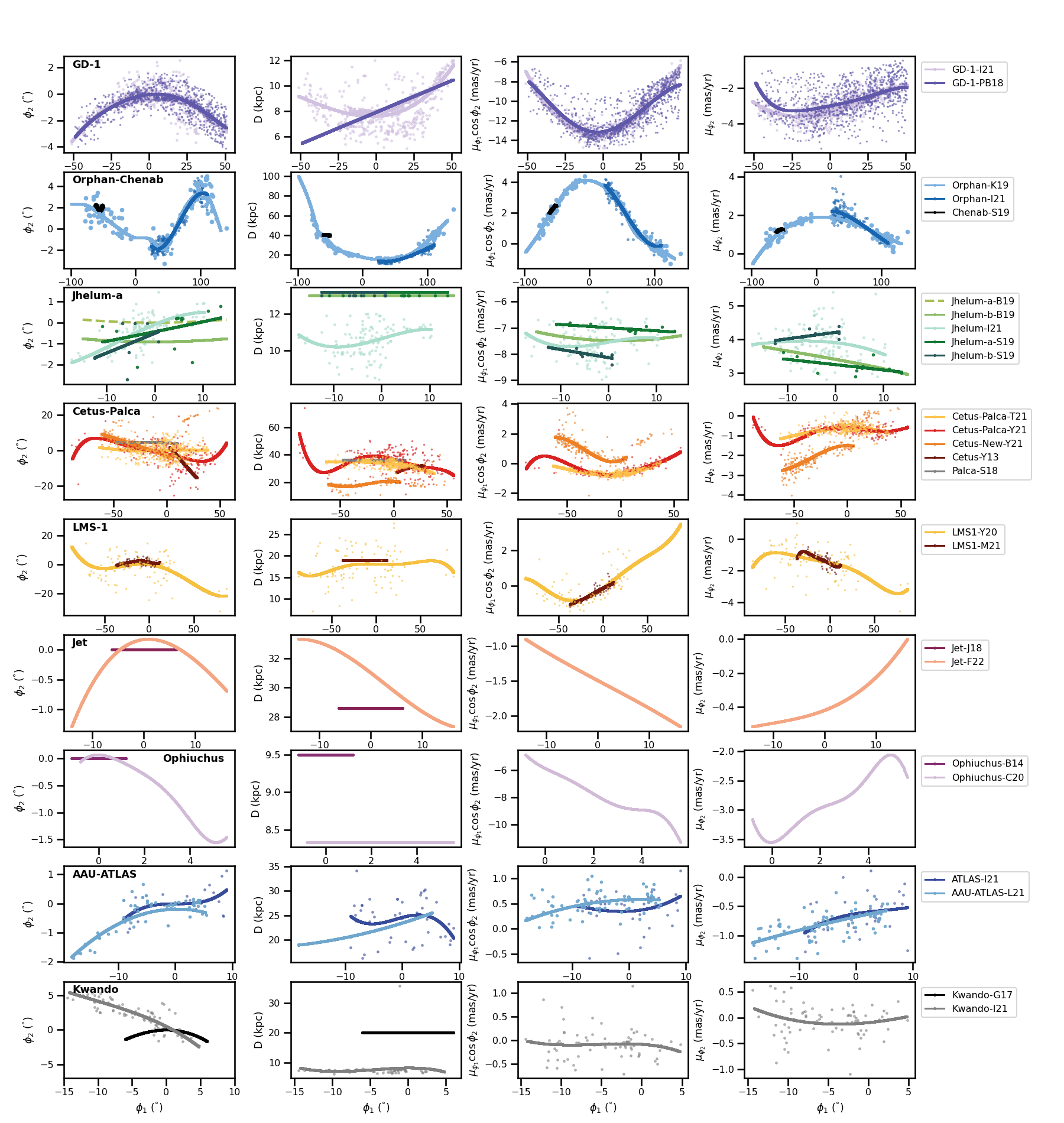
4.1.1 GD-1

For the GD-1 stream (top row) there is remarkable agreement in the celestial and $\mu_{\phi_{1}}$ tracks. Minor differences, e.g. in proper motion are clearly much smaller than the average dispersion of the stars they’re based on. The most significant difference is observed in the distance track. We have assumed for the PB18 track the linear distance gradient the authors proposed since the stream is too distant for Gaia DR2 parallaxes to be useful. The I21 track, on the other hand, includes distances inferred by the STREAMFINDER algorithm Malhan & Ibata (2018) using the observed ${\mathrm{G}}$ , $G_{\mathrm{BP}}$ and $G_{\mathrm{RP}}$ magnitudes from Gaia, and show a parabolic distance gradient. Given its more detailed inferred (rather than assumed) distance gradient track, we set the GD-1-I21 track as the default for the GD-1 stream.

4.1.2 Orphan-Chenab

For the Orphan-Chenab stream (second row) the agreement between the tracks is remarkable, only very minor differences are visible at $\phi_{1}\sim 100\degr$ in distance with the I21 track is $\sim 6$ kpc below the K19 one and at $\phi_{1}\sim 20\degr$ in $\mu_{\phi_{2}}$ with the I21 track having slightly larger proper motion than K19. The agreement in distance is particularly noteworthy, as K19 is derived from photometric distances of RR Lyrae stars and I21 are distances inferred by STREAMFINDER based on the star’s $\mathrm{G}$ magnitude, $\mathrm{G_{BP}-G_{RP}}$ colour and a simple stellar population model (Malhan & Ibata, 2018). Given its much larger extent we set the Orphan-K19 track as the default for the Orphan-Chenab stream.

We have also included Chenab in this comparison, recognised by Koposov et al. (2019) to be a part of Orphan’s southern tail, as clearly illustrated by the agreement of Chenab’s and Orphan’s celestial, distance and proper motion tracks. Hence, we have adopted the Orphan-Chenab name for the stream and take Chenab to be a part of it, set as ‘Off’ in the library.

4.1.3 Jhelum

Jhelum is quite a complex case. Bonaca et al. (2019b) first recognised two separate branches in the Jhelum stream by using deep DES photometry combined with Gaia DR2 proper motions. The data revealed the two branches as separate overdensities in the sky, but with indistinguishable kinematics. Soon after, also using DES and Gaia DR2, Shipp et al. (2019) identified two components in Jhelum, this time in proper motion space and with little difference in the spatial distribution of the two components. Exactly the reverse as Bonaca et al. (2019b). More recently, Ibata et al. (2021) recover a stream they identify as Jhelum using STREAMFINDER with Gaia EDR3.

Figure 5 (third row) shows this quite clearly: the two tracks from S19 (auto-computed by galstreams via polynomial fitting of the member stars) almost coincide in the sky and are clearly separated in both proper motion components. The two tracks from B19 are separated by nearly a degree in the sky and overlap completely in proper motion, so only one line is visible in the last two panels of the figure. In both components, the B19 proper motion track lies approximately in between the two S19 tracks. In the sky, the two nearly parallel S19 tracks cross the B19 ones at a slight angle (the aspect ratio of the figure exaggerates the inclination). The I21 celestial track agrees well with the S19 Jhelum-a/b tracks, while the proper motion tracks agrees with B19. Another aspect to keep in mind is the role of errors and the intrinsic dispersion of the stream in proper motion. B19 note the dispersion in proper motion for both Jhelum components to be relatively large and comparable to the proper motion uncertainty $\sim 0.7$ to $1.2$ $\mathrm{mas\,yr^{-1}}$ ; the I21 members in Figure 5 also show a dispersion of $\sim 1\,\mathrm{mas\,yr^{-1}}$ .

Given these two scenarios, it seems likely that if the two Jhelum components shared a single but long and sinuous track (the B19 case) in the proper motion plane (reflex corrected, Figure 7), this could be mistaken by a Gaussian Mixture Model as two (or more) proper motion components, which statistically would be a random mixture of the two spatial components (the S19 case). If this were the case, it would be akin to the bifurcation of the Sagittarius stream, in which two spatially distinct components appear to have no difference in their proper motion tracks (Ramos et al., 2021a, b, see e.g.), \textcolorblackas mentioned also by (Shipp et al., 2019). \textcolorblackThe addition of radial velocity information as well as a further increase in the precision of proper motions in the next Gaia Data Release will probably elucidate this. In the mean time, as we find the B19 scenario more likely to explain the three sets of observations (B19, S19 and I21), we will set these as the default tracks for the Jhelum-a/b components of the stream, but warn the reader to take this with a grain of salt.

4.1.4 Cetus, Palca and Cetus-Palca

For the Cetus stream, Figure 5 (fourth row) shows four different tracks: the original discovery track Y13, Cetus-Palca-T21, Cetus-Palca-Y21 and Cetus-New, a new branch identified by Yuan et al. (2021). The track for Palca is also shown, as T21 and Y21 claim the Palca and Cetus stream reported in their studies to be related. Their corresponding pole tracks are also shown in Figure 6. The comparison between the celestial tracks shows a complex scenario. Both the $\phi_{1}-\phi_{2}$ plot and the pole tracks show that the Y21, T21 and Palca tracks roughly cross the same are of the sky, but there are systematic differences between the two. The T21 track is parallel to Palca, separated by $\sim 5\degr$ . The Y21 track is inclined with respect to both T21 and Palca, also shown by the fact the I21 pole track –despite being extensive– does not contain either the Palca pole or the T21 pole track, which it only barely overlaps. The better part of these track’s poles (Palca, T21, Y21 and Cetus-New), however, occupy a reasonably well-defined locus in Figure 6, confined to an area with $\sim 10\degr$ -radius. The overall good agreement observed between the Y21 and T21 distance and proper motion’s tracks might suggest they are indeed tracing the same feature, and the differences in their celestial (and pole) tracks might have to do with sampling issues and probable contaminants at the ends of the streams introducing spurious oscillations in the Y21 tracks. The case of Cetus-New seems more clear, as the track is evidently distinct in distance and both proper motions. Finally, The Cetus-Y13 celestial track looks highly inclined with respect to the others and with its pole separated by more than $30\degr$ from the area where the Cetus-Palca poles cluster. Kinematic data could have helped disentangle this, but Cetus-Y13 has radial velocity information but no proper motion data, while the Cetus-Palca Y21 and T21 tracks have proper motion but no radial velocity data. Since a definitive association between several of these tracks seems unclear, we will keep the Cetus-Y13 track as the default for Cetus; the T21 as the default for the main branch of Cetus-Palca, as it is the most stable track with the best behaved pole track; and Cetus-New as a separate branch under that name. The Palca track is also kept as a separate stream.

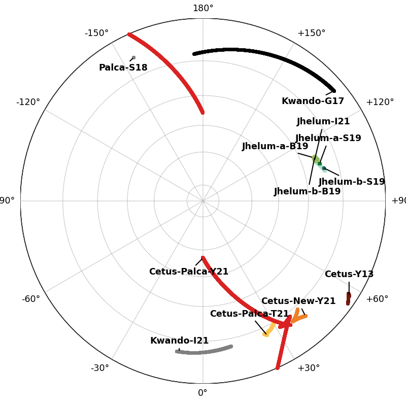
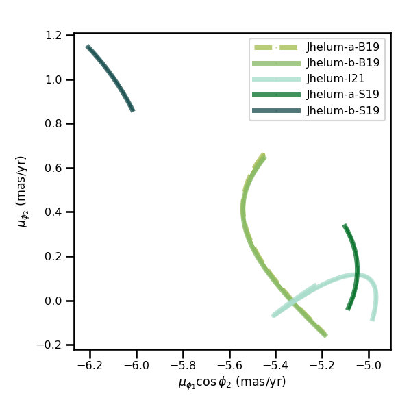
4.1.5 LMS-1

For LMS-1 there are two available tracks, the discovery track LMS1-Y20 and the follow-up by M21, shown in Figure 5 (penultimate row). There is also radial velocity information for both, shown in Figure 8. Both tracks show excellent agreement in every coordinate, sky, distance, proper motions and radial velocities and, although there is overlap in $\phi_{1}$ , there are no objects in common between the two studies. Since the Y20 track spans a much larger range of $\phi_{1}$ , we set this as the default for the LMS-1 stream.

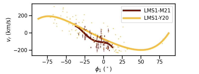
4.1.6 Jet

For Jet there are two available tracks, the discovery track Jet-J18 and the follow-up by F22, shown in Figure 5 (sixth row) which includes proper motion data and extends the stream’s track by $\sim 20\degr$ in length. Although the new F22 track differs from the great-circle discovery track, this discrepancy is only by $\sim 0\aas@@fstack{\circ}1$ , so there is good agreement. There is, however, a significant discrepancy in the distance, with the F22 track being systematically more distant by up to $\sim 4$ kpc. Given the much larger extent and proper motion data available in the F22 track, we set this as the default for the Jet stream.

4.1.7 Ophiuchus

\textcolor

black Similarly to Jet, there are two available tracks for Ophiuchus: the discovery track Ophiuchus-B14 and the follow-up by C20, shown in Figure 5 (seventh row) which includes proper motion data and extends the stream’s track by $\sim 10\degr$ in length. The celestial tracks coincide very well. In the distance tracks there is a $\sim 1$ kpc discrepancy, with the B14 track having the more distant estimate. Given the much larger extent and proper motion data available in the C20 track, we set this as the default for the Ophiuchus stream.

4.1.8 AAU-ATLAS

\textcolor

black The two available tracks for the ATLAS branch of the ATLAS-AliqaUma stream are shown in Figure 5 (penultimate row), together with members from I21 and spectroscopically confirmed members from Li et al. (2021). The two tracks show excellent agreement in the sky, distance and proper motion spaces. The AAU-ATLAS-L21 track extends $\sim 5\degr$ further than the ATLAS-I21 track⁸⁸8Note that the ATLAS-I21 track had initially been dubbed Víd in the preprint version of I21. and includes published radial velocities, hence it is set as the default for the ATLAS branch of the AAU stream.

4.1.9 Kwando

\textcolor

black The Kwando-G17 track from the Grillmair (2017b) discovery paper is compared against the Kwando-I21 track in the last row of Figure 5. Their heliocentric pole tracks are compared in Figure 6. There is significant disagreement between the two celestial and distance tracks. In the sky, the I21 track intersects the G17 one at a significant inclination, confirmed by the difference in their (heliocentric) pole tracks of well over $20\degr$ in pole latitudes. In distance, the I21 track is located at half the distance of the G17 track. Kwando is one of several streams found using photometry alone pre-GaiaDR2 (e.g. streams from, but not limited to, Bernard et al., 2016; Grillmair, 2017a, b; Mateu et al., 2018) that have lacked further follow-up (see discussion in Sec. 5.1). Further studies will be required to clarify the two (separate) issues of robustness of the Kwando stream and whether the association of Kwando-I21 to the Kwando stream is correct or if it corresponds to a new stellar stream⁹⁹9The Kwando-I21 track had initially been dubbed C-9 in the preprint version of I21.. In the mean time, we have kept the G17 as the default for the Kwando stream, because the Kwando-I21 association with it is unclear.

4.2 Streams associated with surviving globular clusters

The celestial, distance and proper motion tracks for stellar streams that are associated with surviving globular clusters and have multiple track realisations, are shown in Figures 9 and 11. Figure 9 shows, from top to bottom, the multiple tracks for clusters Pal 5, NGC 3201-Gjöll, M92, M5 and M68-Fjörm and Figure 11 shows the tracks for NGC 288, NGC 2298, NGC 5466, M2 and $\omega$ Cen-Fimbulthul.

4.2.1 Pal 5

For Pal 5, the PW19 and I21 tracks have very similar extents in $\phi_{1}$ and coincide remarkably well in the sky. The S21 track extends the cluster’s leading tail by $\sim 7\degr$ compared to the previous ones, however, it lacks distance and proper motion information. In distance and proper motions there is overall agreement between the PW19 and I21 tracks around the position of the cluster ( $\phi_{1}\sim 0\degr$ ) and the leading tail ( $\phi_{1}>0\degr$ ), but they start to differ in proper motions in the trailing tail at $\phi_{1}\lesssim-5\degr$ . The PW19 is based on RR Lyrae stars whose distances are more precise and require no inference involving the orbit, as do the STREAMFINDER distances in I21. The PW19 data is also more constraining as revealed by the lower dispersion in the distance and proper motion tracks. Hence, we set the PW19 track as the default for Pal 5. We note, however, that since the two studies are based on different stellar populations these differences could be physically meaningful.

4.2.2 NGC 3201-Gjöll

For NGC 3201 the two available tracks (P21 and I21, second row of Fig. 9) coincide very well, in the sky, distance and in both proper motions. The I21 track’s extent is of about $10\degr$ and centred around the cluster, compared to $>100\degr$ length for the P21 track. In their work, Palau & Miralda-Escudé (2021) recognised the Gjöll stream (Ibata et al., 2019b) as part of the NGC 3201 tidal tail identified with their algorithm. An excellent agreement is clearly seen between the two celestial, distance and proper motion tracks in the figure. We will set the much longer P21 track as the default for the NGC 3201-Gjöll stream. The Gjöll track is set as ‘Off’ and ascribed to NGC 3201-Gjöll.

4.2.3 M92

For M92 the S20, T20 and I21 tracks (third row in Fig. 9) intersect the cluster position in the sky. I21 and S20 coincide at positive $\phi_{1}$ , but the S20 track departs from the I21 at negative $\phi_{1}$ . Still, it is a minor deviation considering it is reasonably within the dispersion of the I21 track stars. The T20 track does not agree with either I21 or S20 –even considering the dispersion of I21 members– with the largest mismatch again at negative $\phi_{1}$ . Since the S20 and T20 tracks contain no kinematic information, the I21 is set as the default for M92.

4.2.4 M5

For M5 (fourth row in Fig. 9) there are three available tracks: S20 limited to the celestial track and intersecting the cluster position; and G19 and I21, both with full sky, distance and proper motion data but neither crossing the cluster’s position. The celestial I21 track agrees with G19 for the most part, with the angle changing somewhat at the positive $\phi_{1}$ end; but note that the aspect ratio of the figure is probably exaggerating the differences. The S20 interestingly could be the extension of the stream at negative $\phi_{1}$ . To better judge the differences between the three celestial tracks, we compare their corresponding (heliocentric) pole tracks, as shown in Figure 10 in a north polar azimuthal projection. This shows the I21 and G19 poles overlap for the most part, but the S20 does not, indicating a completely different –and highly varying– orbital plane. This casts doubt as to the likelihood of the S20 track truly being associated to the M5 stream. In the proper motion tracks there seem to be some differences between I21 and G19, but being so much shorter in comparison to G19 the more meaningful comparison would be of its mean proper motion which does seem consistent. The distance tracks, however, are entirely inconsistent with I21 located a nearly half the distance of the G19 track, \textcolorblackbut, although separated more than $30\degr$ away from the cluster, much closer to the Baumgardt & Vasiliev (2021) distance for the cluster used in the S20 track. Given its much larger extent we set the G19 track as the default for the M5 cluster, but recommend to use its distance information with caution.

4.2.5 M68-Fjörm

For M68 (last row in Fig. 9), the association of Fjörm and M68, already pointed out by Palau & Miralda-Escudé (2019), is also seen here in the overall excellent agreement between the tracks \textcolorblackin the sky and both proper motion components. However, note the disagreement between the two distance tracks at $\phi_{1}\lesssim 30\degr$ , where the I21 predicts a much shorter distance than P19. We caution that in both samples, there is a sharp decrease in the number of member stars at that $\phi_{1}$ range precisely. It is also worth noting the disagreement between both tracks and the cluster distance from Baumgardt & Vasiliev (2021). On the other hand, at $\phi_{1}\gtrsim 30\degr$ the two distance tracks agree well, despite the caveat mentioned in Sec. 3.2 about P19 distances having been computed from the reciprocal of the reported parallax.

When compared to the M68-I21 track, there is significant disagreement. The Fjörm-I21 celestial track (based on the candidates reported in their Table 1) and the M68-P19 track both intersect the cluster position in the sky, but M68-I21 crosses the P19 track at an angle. Again, to avoid being mislead by the aspect ratio of the plot, we compare the corresponding pole tracks in Figure 10. This shows the two tracks have very minor overlap, indicative of significantly different orbital planes, further supported by systematic differences observed between the two tracks in both proper motion components. The M68-I21 track has a significantly larger proper motion (over 4 times larger) than the cluster even at similar $\phi_{1}$ , where some overlap would be expected.

These discrepancies cast doubt into the association of the M68-I21 track with the M68 cluster and could be pointing to this feature being a distinct new stream. \textcolorblackRadial velocity information would help settle the matter, but is currently only available for the Fjörm-I21 track, but not for the M68-P19 or the M68-I21 tracks. The M68-P19 track is set as the default for the M68-Fjörm stream. For naming clarity, the Fjörm track is set as "Off" and ascribed to the M68-Fjörm stream, given its perfect agreement with the M68-P19 track. The M68-I21 track is set as "Off" and not ascribed to M68-Fjörm \textcolorblackuntil further information is available and the proper motion discrepancy is resolved.

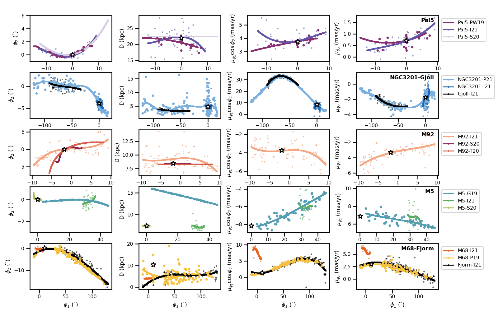
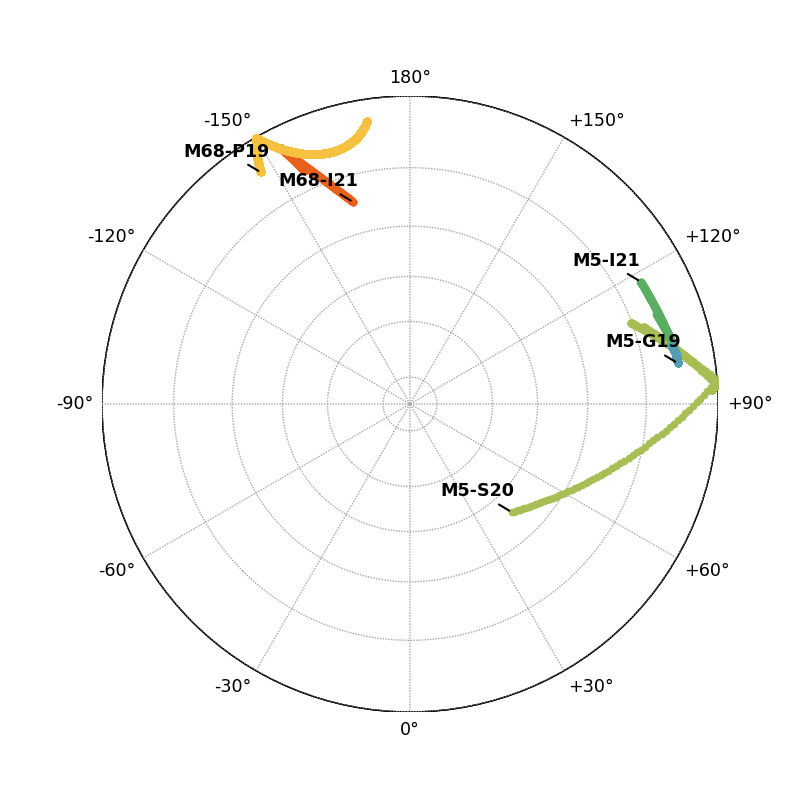
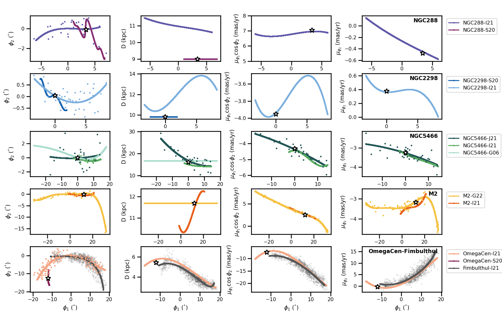
4.2.6 NGC 288, NGC 2298

For these two clusters there are tracks available from I21 and S20, as shown in the first two rows of Figure 11. In both cases the I21 tracks trace the stream for a longer span and include proper motion data; S20 tracks are limited to information in the plane of the sky. The two sets of tracks for NGC 2298 show reasonable agreement, within the dispersion. The case of NGC 288 is interesting, the S20 track is much more wiggly and has a drop towards negative $\phi_{2}$ that seems unphysical at first, but coincides with the I21 stars in that region. The analysis of kinematic data in the S20 overdensity track would help confirm their membership to the cluster’s tails. \textcolorblackNote also the significant difference in the NGC288-I21 distance and the Baumgardt & Vasiliev (2021) distance estimate for the cluster, of nearly 2 kpc. In the other two cases there is also a slight discrepancy of $<1$ kpc.

In both cases the I21 track is set as the default for each cluster, given the more extensive coverage and availability of proper motion data.

4.2.7 NGC 5466

\textcolor

blackThere are three different tracks available for NGC 5466: the discovery track from G06, with no distance gradient or proper motion data, and the I21 and J21 tracks both with distance and proper motion data. The I21 and J21 tracks agree very well in all coordinates, with the J21 track having a much larger extension (by $\sim 20\degr$ , particularly tracking the stream’s tail in negative $\phi_{1}$ , not present in I21). The G06 celestial track shows a better agreement with the previous two in $\phi_{1}>0\degr$ , while at $\phi_{1}<0\degr$ the disagreement is larger but never exceeds $\sim 2\degr$ . As noted in Sec. 3.2, the G06 distance was assumed to be the mean cluster distance and therefore, the disagreement is expected. Note also how the I21 track is limited to $<10$ kpc, a distance limit of the STREAMFINDER algorithm, as we will discuss in Sec. 5.3 ). For this stream, due to its length and 5D data availability, the J21 is set as the default.

4.2.8 M2 (NGC 7089)

As discussed by Grillmair (2022), there is excellent agreement between the I21 and G22 tracks for M2, as shown in the fourth row of Figure 11. The G22 extends the observed length of the tail by over $30\degr$ and includes proper motion data and is set as the default for this cluster. We caution that at this point it does not include information about the distance gradient, which is predicted by Grillmair (2022) to be significant based on integration of the cluster’s orbit. This information is available in the I21 track showing a gradient of $\sim 2$ kpc in its $20\degr$ span.

4.2.9 $\omega$ Cen-Fimbulthul

The bottom row of Figure 11 shows the I21 track for the $\omega$ Centauri (NGC 5139) cluster constructed from members published in Ibata et al. (2021) and compared to the Fimbulthul stellar stream first found by Ibata et al. (2019b) and identified by Ibata et al. (2019a) as the long sought stream of $\omega$ Cen. The agreement between these two tracks is, therefore, expected and is shown here only to illustrate the coverage of the new track (I21) with respect to Fimbulthul and the cluster itself. As the plot shows, the cluster is separated several degrees from the celestial track, while it does coincide with the track in both proper motion components. The S20 track, with only celestial data, is also shown in the first panel, it joins with the cluster, by construction as the search in Sollima (2020) was targeted around globular clusters, and seems disjoint from the I21 track. In this case, again we set the I21 track as the default for the $\omega$ Cen-Fimbulthul stream and set Fimbulthul as ‘Off’ and not considered a separate stream any further.

5 Global Properties of the System of Stellar Streams

In this section we will discuss global properties of the galstreams library. Table 1 provides a summary of the main characteristics of the total 126 stream tracks implemented. As discussed in the previous section, a single track was selected as the default one for each of the 95 unique stellar streams in the library, these are indicated as ‘On’ in the table.

5.1 Available Information

Figure 12 summarises the available information for the 95 stellar streams implemented in the library. In order to be included in the current version, a stream must have a celestial track and minimal distance information (e.g. a mean distance or distance at an anchor point). However, the degree of detail with which this is reported varies. In its first version, most of the streams in galstreams were assumed to be great-circles and their tracks implemented under this assumption. In the current version, over three quarters of the streams in the library (77%) have a detailed celestial track, the remainder are great-circles by construction.

Somewhat surprisingly, only about half (55%) the streams have sufficiently detailed distance information to implement a distance gradient in the track, for the remaining 45% only a mean distance is provided. This last percentage does not include cases in which a constant distance is observed to be a good approximation for the stream, these cases are indicated in the library as having distance gradient information. This deficit is partly due to a lack of follow-up on many streams (e.g. PS1-A/E, Corvus, Molonglo, Murrumbidgee, etc.) detected before Gaia DR2, and can also be justified for some of the shorter streams (e.g. Pal 15, Eridanus), but for the majority it reflects how challenging and observationally demanding it remains to estimate distances for these relatively low-contrast structures when outside the Gaia-sphere.

Conversely, well over half the streams (64%) do have detailed proper motion tracks, an achievement possible thanks to the Gaia DR2 and EDR3 releases (Gaia Collaboration et al., 2018, 2021). Most streams that do not have proper motion information were discovered prior to the Gaia data releases and have not been revisited, so there is a clear opportunity to complement the available information for the majority of those within the reach of Gaia. Finally, as was natural to expect, only a small portion (7%) of the streams have radial velocity information available.

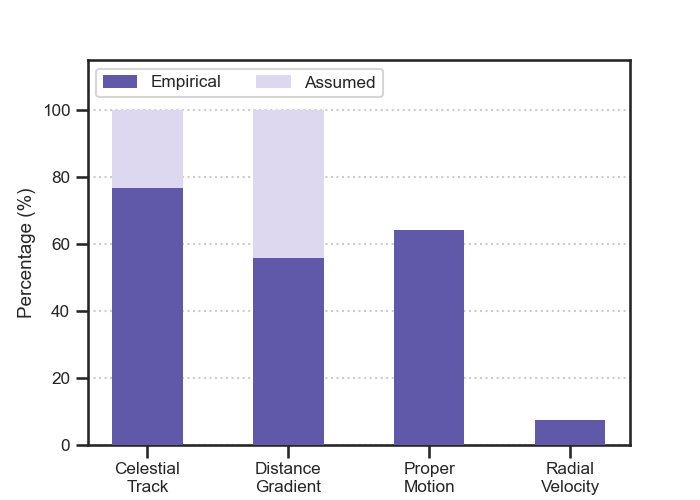
5.2 Celestial Distribution

Figure 1 shows in a Mollweide projection map in Galactic coordinates, the celestial tracks of the 95 unique stellar streams (i.e. no repetition), out of the total of 126 tracks implemented in the galstreams library. The map clearly shows the observational bias against the detection of stellar streams near the Galactic plane. \textcolorblackThis bias is anticipated and expected as current detection techniques will struggle to disentangle the faint signature of a stellar stream against the vastly more numerous disc background, and subject to crowding effects and the high and non-uniform extinction affecting photometric depth and completeness. Only a few streams -Sagittarius, Orphan-Chenab, LMS-1 and NGC 3201- have been unequivocally traced on both sides of the plane, and all cross it almost perpendicularly, a significant off-plane component of motion facilitating detection against the disc background.

A 3D view in cartesian Galactocentric coordinates is shown in Figure 13. The bias in the distribution in favour of nearby streams ( $\lesssim 20$ kpc) is evident in the clustering observed around the Sun’s position (-8.12 kpc). Another apparent clustering of several streams is found in the direction of the Magellanic Clouds, but at shorter distances. The streams in this region are Vid, NGC1261 (Ibata et al., 2021), Cetus/Cetus-Palca (Yam et al., 2013; Thomas & Battaglia, 2021), Willka Yaku, Tucana III, Atlas-AliqaUma, Ravi (DES, Shipp et al., 2018), Murrumbidgee, Molonglo, Kwando, Orinoco (SDSS, Grillmair, 2017b). The group is a mix of streams discovered by different groups, but all except for the first two, discovered with STREAMFINDER, involved an implementation of matched-filtering. It will be interesting to explore to what extent is this clustering real. Bonaca et al. (2021) has already identified groups of streams with a common origin by means of orbital clustering, but only 2 out of the streams in this group are included in that analysis (Atlas-AliqaUma and Ravi, found to be associated with differnt groups) since there is no proper motion information available for the SDSS streams and the data for the rest was published afterwards.

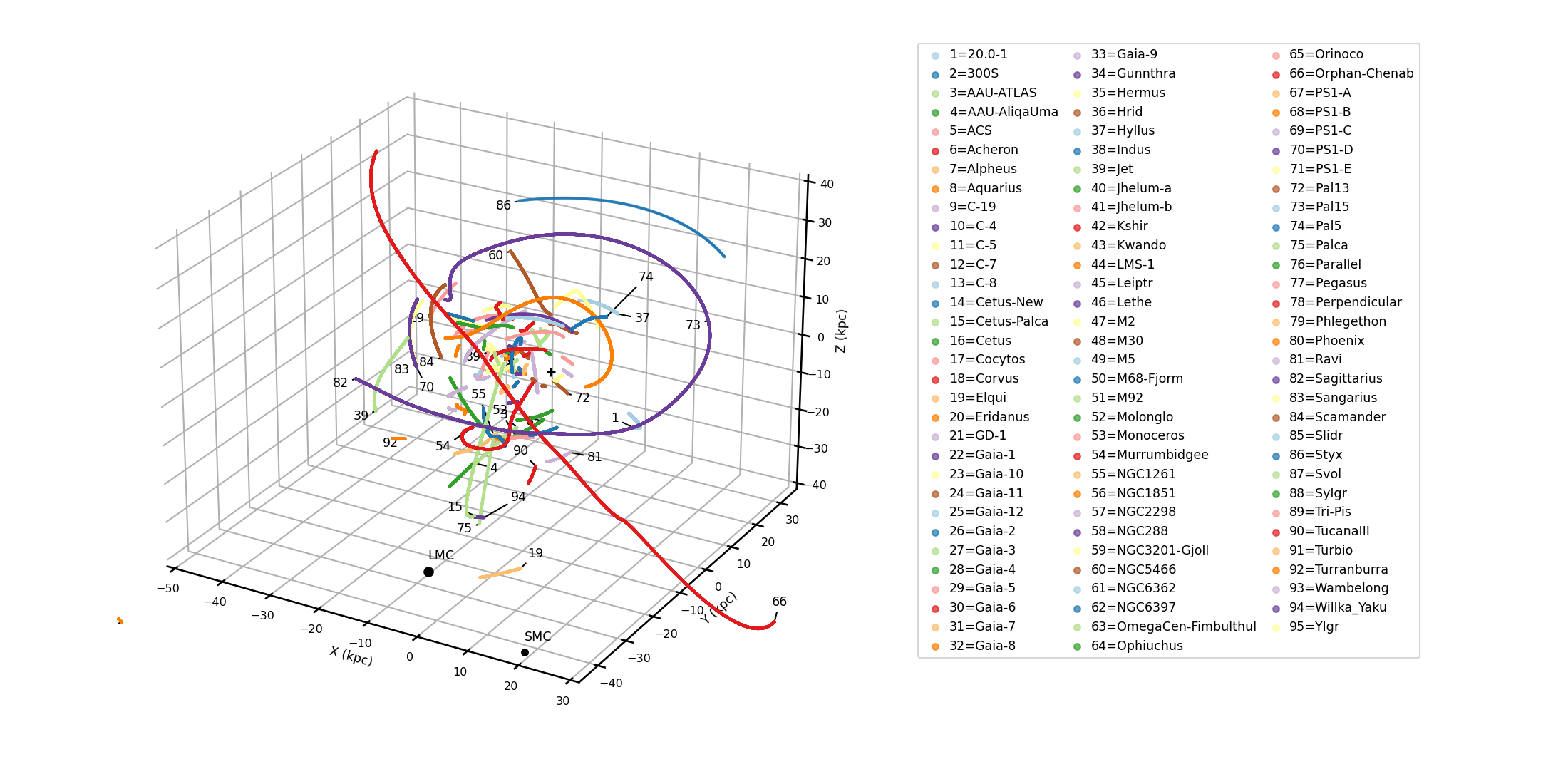
5.3 Distance Distribution

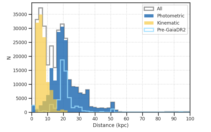
Figure 2 showed a plot of all stream’s distance tracks in the library as a function of Galactic longitude. This information is also shown summarised in Figure 14, in which all (unique) celestial tracks have been aggregated into a single (heliocentric) distance distribution, \textcolorblackeach having been populated with a uniform spacing along the track. This figure essentially corresponds to a histogram of Figure 2 along the y-axis. These two figures show that the vast majority of streams are located within 30 kpc (95), with only five streams (Styx, Cetus-Palca, Elqui, Orphan-Chenab and Sagittarius) having part or all of their track in the 30-40 kpc range and Eridanus being the farthest located at a mean $\sim 95$ kpc.

\textcolor

blackFigure 14 presents two clear peaks at $\sim 7$ kpc and $\sim 20$ kpc. This observed bimodal distribution is produced by the combination of two effects: the real distance distribution of stellar streams plus the effects of observational biases involved in the main two types of methods used in the identification of the streams. First, the distribution of streams in distance is expected to decrease with distance as tidal forces dwindle and systems are less prone to losing stars (see e.g. Figs. 11 and 14 of Mateu et al., 2017). On the other hand, are the selection effects of the methods used in finding the stellar streams. In this case, selection effects are quite different depending on whether or not kinematic information was required by the detection method. This is illustrated in Figure 14, where the distributions of streams detected based on kinematics (those from Malhan & Ibata, 2018; Palau & Miralda-Escudé, 2019; Ibata et al., 2019b; Grillmair, 2019; Palau & Miralda-Escudé, 2021; Jensen et al., 2021; Ibata et al., 2021; Grillmair, 2022) or on photometry are shown separately (light yellow and dark blue histograms respectively). The figure shows that for streams discovered using kinematic information, the selection function decreases with distance and has a sharp drop-off at $\sim 12$ kpc. This drop-off is driven by the limits of the volume in which Gaia’s proper motions are precise enough for the methods to work. Combined with the decrease in distance, this produces the first peak at shorter distances ( $<10$ kpc).

\textcolor

blackConversely, streams detected photometrically clearly dominate at large distances ( $\gtrsim 15$ kpc). The distribution shows a peak at $\sim 20$ kpc¹⁰¹⁰10This prevalence of streams at $\sim 20$ kpc was already noticeable in galstreams v0.1, in which all streams had been detected with photometry alone (pre-dating Gaia DR2). produced by the combination of an increasing probability of detection at larger distances, due to photometric methods being biased against nearby streams that –in projection– would be more diffuse and hence more difficult to detect, combined with the declining number of expected streams as a function of distance. It is clear, then, that the selection functions of streams with/without kinematics, are not only different but almost complementary. This also suggests a sweet-spot at distances of $\sim 10-15$ kpc where there are likely more streams to be found, since the two mainstream method families for stream finding have lower detection probabilities at this distance range but the number of expected streams hasn’t yet significantly declined.

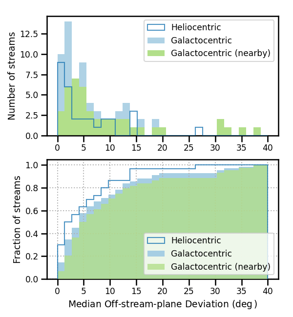
5.4 Great circle deviations

In Section 5.1 we showed 22 (23%) of the stream tracks in the library are great circles by construction. The remaining streams have enough data available for more detailed tracks to be constructed empirically, which may or may not be well fit by great circles. Here we will assess how well these streams are represented by great circles, in both the heliocentric and galactocentric reference frames.

There is no particular physical reason for the projections of streams to lie along great circles for a heliocentric observer. Instead, for a galactocentric observer, stellar streams formed in a potential with spherical symmetry would have constant angular momentum and, thus, remain confined to a constant plane. \textcolorblackFor this observer such a stream, in projection, would look like a great circle, however complex its radial structure may be (see e.g. Johnston et al., 1996; Mateu et al., 2017). Breaking of spherical symmetry will cause the orbital plane to precess and the stream to deviate from a great circle, even for a Galactocentric observer. In the Milky Way, the Sagittarius stream’s orbital plane presents a small rate of precession ( $\lesssim 10\degr$ Belokurov et al., 2014), showing that although not perfectly spherical, the (galactocentric) great circle approximation should be a good one for streams in the outer halo ( $\gtrsim 25$ kpc). In addition, the difference in the projected view between the heliocentric and Galactocentric observers becomes ever smaller as distance to the stream increases \textcolorblackand the Sun-Galactic-Centre distance becomes negligible..

A large prevalence of great circle streams in the heliocentric frame, particularly for nearby streams, would thus be indicative of an observational bias in the detection techniques \textcolorblacksince there is no physical reason to expect it. Figure 15 shows the distribution (top panel, cumulative in the bottom panel) of the median deviation of each stream’s pole track from its mid-pole (see Sec. 3.1) for a heliocentric (open) and Galactocentric observer (filled). Note that in these plots each stream contributes only a single point. For a heliocentric observer the distribution (open) shows 60% of the stream’s tracks deviate less than $5\aas@@fstack{\circ}5$ from their mid-plane; about half are less than $3\degr$ wide (on median). For a galactocentric observer the distribution as a whole is similar in shape, but shifted towards slightly larger values indicating larger deviations from a great circle, 60% show deviations $\sim 8\degr$ and half deviate just under $5\aas@@fstack{\circ}5$ . The figure also shows the distribution of Galactocentric deviations for the nearest streams (light green histogram), defined as those with stars at distances $<15$ kpc. This shows that, as expected, the tail of the distribution towards large deviations is dominated by nearby streams: i.e. nearby streams are less likely to be well represented by great circles from a galactocentric perspective. Vice versa, the complementary distribution for more distant streams (not shown) is dominated by smaller deviations, meaning more distant streams are indeed similarly thin from either point of view. This indicates there is no evident bias towards the detection of (heliocentric) great circle streams.

5.5 Proper motion misalignment, angular momentum and pole tracks

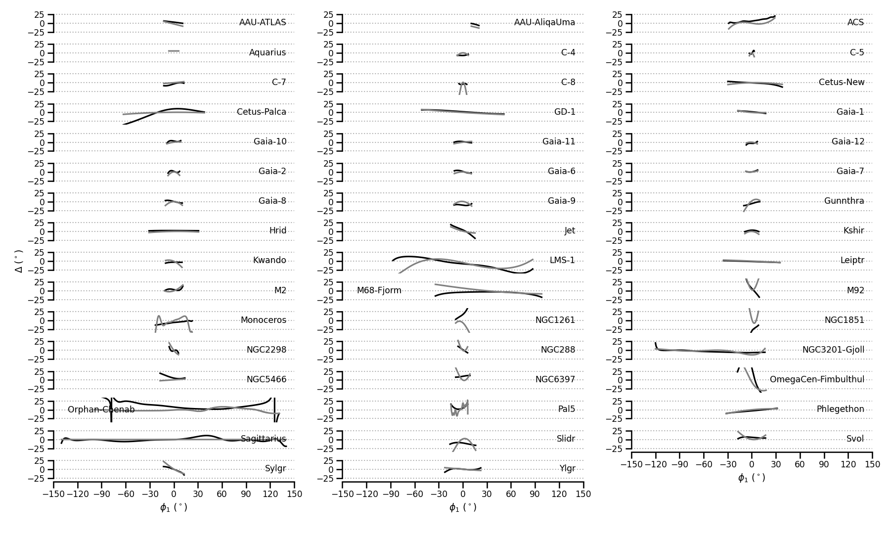
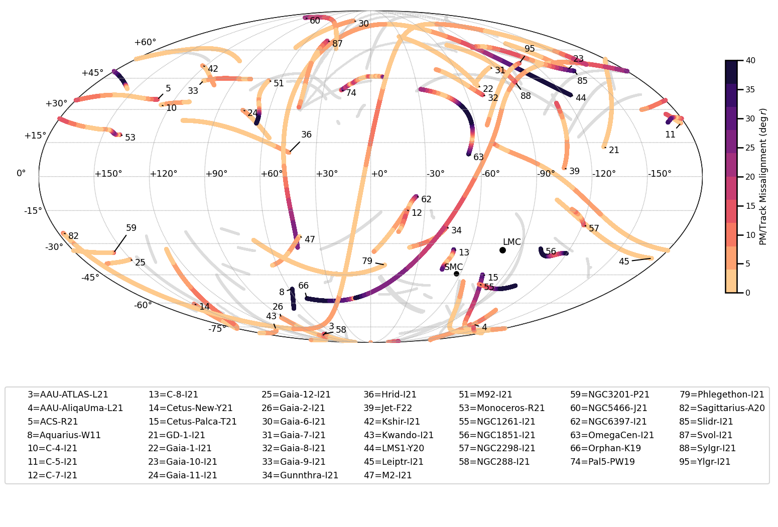
The availability of proper motion tracks for over half the library makes it possible to compute the angular momenta along the track for a large number of streams, \textcolorblackalbeit only in a heliocentric reference frame. It is convenient at this point to report the angular momentum in a heliocentric frame at rest with respect to the GSR, because in this reference frame the radial velocity has no contribution to the angular momentum and currently only 5 streams have radial velocity information in addition to proper motions, necessary to get the full angular momentum vector in the GSR (see Sec 3.1).

In an undisturbed stellar stream, stars are expected to be moving mainly along the stream, which approximately traces the orbit of the progenitor (Binney, 2008). In such a case, the stream star’s velocity, and therefore its proper motion in projection, is expected to be tangent to the stream track itself ¹¹¹¹11See Sanders & Binney (2013) for a discussion of the limitations of this approximation.. However, analyses of Gaia DR2 data have revealed several cases in which the proper motions are significantly misaligned with the stream’s track (Erkal et al., 2019; Shipp et al., 2019). First observed in the southern tail of the Orphan-Chenab stream (Koposov et al., 2019; Erkal et al., 2019), Erkal et al. showed the proper motion misalignment can be attributed to the dynamical effect of the LMC during a recent (<350 Myr ago) close encounter with the stream. Shipp et al. (2019) have observed a similar effect in several of the DES streams (Indus, Jhelum, and to a lesser extent Aliqa Uma and Turranburra), which they also attribute to the effect of the LMC (Shipp et al., 2020).

For the stellar streams in galstreams that have proper motion and distance track information available, we can provide a systematic survey of proper motion misalignment. This could be visualised in two different but equivalent ways: by comparing the tangent to the stream track $d\phi_{2}/d\phi_{1}$ with the ratio of proper motions $\mu_{\phi_{2}}/\mu_{\phi_{1}}$ along the track (corrected for the solar reflex motion), as in Erkal et al. (2019); or by measuring the angular distance between the angular momentum and the pole vector along the track. For an unperturbed stream, in the first case, the ratio of proper motions should coincide with the slope of the tangent along the track $d\phi_{2}/d\phi_{1}$ ; in the second case, the pole and angular momentum vectors should be co-linear. Using the first visualisation, Figure 16 shows the proper motion¹²¹²12To correct for the solar reflex motion, we assume $(X,Y,Z)_{\odot}=(8.122,0.0,0.208)$ kpc (Gravity Collaboration et al., 2018; Bennett & Bovy, 2019) and $V_{\odot}=(12.9,245.6,7.78)$ km s^-1(Drimmel & Poggio, 2018; Gravity Collaboration et al., 2018; Reid et al., 2014) for the position and velocity of the Sun in the Galactic Standard of Rest, respectively. and stream tangent tracks (black and light grey, respectively) for the 45 streams with proper motion and distance gradient data. In this figure all the tracks are shown in the same horizontal and vertical scales (in degrees) to make the comparison easier between different streams. Figure 18 in Appendix A shows the alternative visualisation, the angular distance between the angular momentum and pole vectors, which corresponds to the absolute difference between the tracks in Figure 16. Figure 19 shows a map in heliocentric Galactic coordinates of the angular momentum and pole tracks for each stream. In these plots, only stellar streams with distance gradient information are shown. Streams with only mean distances available are excluded because proper motions used to judge the misalignment must be corrected for the solar reflex motion. Since this correction is distance dependent, a spurious misalignment can appear if a significant distance gradient is misrepresented by assuming only a mean distance.

Some very long streams with no misalignment are, e.g., NGC3201-Gjöll (P21 track shown), Phlegethon and Leiptr in addition to well-known cases like GD-1 (Price-Whelan & Bonaca, 2018; Grillmair & Dionatos, 2006a). On the other hand, the misalignment is evident in the mismatch between the proper motion ratio and stream tangent track in the reported cases of Orphan-Chenab, Jhelum, Indus, Elqui, Turranburra and AAU-AliqaUma (Erkal et al., 2019; Shipp et al., 2020) as well as in some parts of the Sagittarius track (Vasiliev et al., 2021, see), \textcolorblackalthough it exhibits very little misaligment for the most part; and also in the Cetus-Palca stream, Slidr and LMS-1 and M68-Fjörm, previously unreported.

In the case of Cetus-Palca-T21 and M68-Fjörm the misalignment happens at one end of the stream (similar to the Orphan-Chenab case). The detection of misaligned proper motions in Cetus-Palca-T21 appears robust, its track is fairly stable and based on members all along the track, the observed misalignment is substantial (similar to that in Orphan-Chenab) and the distance track is robust as it is based on photometric standard-candle distances of Blue Horizontal Branch stars (see details in Cetus-Palca-T21), so it is unlikely to be a distance-related effect. The case of M68-Fjörm is also one of apparently high confidence, the two tracks are based on independent detections by Ibata et al. (2021) and Palau & Miralda-Escudé (2019), yet the misalignment observed in the two cases is nearly identical (only the latter is shown). For LMS-1, on the contrary, we caution that the misalignment is observed at the ends of the track where there are fewer members to constrain its shape (see Sec. 4, Fig. 5), compared to the central part ( $|\phi_{1}|<50\degr$ ) where the two tracks agree very well.

Other, much shorter streams, also show signs of proper motion misalignment at the ends of the track (Gaia-8, NGC 1261, M92, NGC 1851, NGC 6397, Slidr, Svöl, Sylgr, Vid, Ylgr). Some cases should be taken with caution and are worth revising, e.g. C-8, Slidr, Sylgr, in which the misalignment could be due to a poorly constrained celestial (or distance) track if there are few members in the stream as a whole (C-8) or at the end where the misalignment is most prominent (Slidr, Sylgr).

Figure 17 illustrates the spatial distribution of proper motion misalignment in a Mollweide projection map in Galactic coordinates, where the colour coding is proportional to the absolute difference (in degrees) between track slope computed from the proper motion ratio and tangent along the track. The area in the southern Galactic hemisphere close to the LMC and SMC where many streams (but not all, see e.g. Willka Yaku) are perturbed is evident. The perturbed tail of the Cetus-Palca stream and NGC 1261 are also around this region. In the northern Galactic hemisphere, the perturbed end of M68-Fjörm coincides (in projection) with a similarly perturbed end of $\omega Cen$ -Fimbulthul; a bit further north, also Gaia-8 shows a perturbed end. The perturbed ends of Slidr, LMS-1 and Sylgr are also in a similar region; bearing in mind the most uncertain end of LMS-1, the one with fewest member candidates, is the end that crosses the Galactic disc, opposite to this one. Several other streams are located in this region, but do not have proper motion information available (shown in grey); these would be interesting to target in a search for any other signs of proper motion misalignment in this area and might provide useful dynamical constraints if used simultaneously in orbital fitting.

6 Summary

Nearly a hundred stellar streams (95) have been found to date around the Milky Way and the number is rapidly growing. In this work we have combed the literature to collate the angular position, distance, proper motion and radial velocity data available for all published streams and stream candidates, \textcolorblack for which we provide 3D ( $126$ ), 5D ( $61$ ) and 6D ( $7$ ) stream tracks where available in a homogenised format in the galstreams library. The library contains 126 tracks with up to 6D information, corresponding to 95 unique streams in our Galaxy, together with a series of computed attributes and utilities, such as stream coordinate frames, end points, pole vector and pole tracks in the heliocentric and Galactocentric reference frames, heliocentric angular momentum tracks and polygon footprints.

An overview of the latest information available for each stellar stream shows that a remarkable almost two thirds of the streams already have proper motion tracks available, thanks to data from Gaia DR2 and EDR3. \textcolorblackThe distance distribution of the streams separated by whether the identification technique used to find them required proper motion data or not (Fig. 14) showed clearly that kinematically detected streams are biased toward short distances ( $\lesssim 10$ kpc) with a peak at $\sim 7$ kpc, while photometrically detected streams are biased toward larger distances ( $\gtrsim 12$ kpc) with a peak at $\sim 20$ kpc. The observed peaks in the distance distribution are clearly due to selection effects, not to be confused with real physical features. Further, there is potential to unearth new stellar streams in the distance range $\sim 10-15$ kpc so far disfavoured by stream finding techniques with widespread use.

Perhaps surprisingly, almost half the streams in the library ( $45\%$ ) are lacking enough information to represent a distance gradient and are implemented with only a mean distance estimate for the full stream. In some instances even these are only rough approximations to a distance estimate. This deficit is due to a lack of follow-up on many stream candidates after their first publication, particularly for streams discovered before Gaia DR2. As we have shown in Sec. 5.3, pre-Gaia DR2 streams are mostly distant ones ( $\gtrsim 15$ kpc), beyond the reach of Gaia parallaxes. For these, photometric distances will play a key role in providing distance gradient measurements, either by the use of standard candle tracers -e.g. RR Lyrae or Blue Horizontal Branch stars- or by less precise isochrone fitting of colour-magnitude diagrams. Since distance information is required for dynamics and ensemble studies of stellar streams are highly desirable to the Galactic dynamics community, efforts to provide consistent distance gradient measurements for all known streams, ideally based on a common distance scale, will be a highly valuable contribution.

The galstreams library is served as a Python package publicly available via a GitHub repository and a summary of the streams’ properties and information available in the compilation for each track is presented here in Table 1.

Table 1: Summary attributes for the tracks available in galstreams.

StreamName	TrackName	InfoFlags	Imp	On	Length	$\alpha_{i}$	$\delta_{i}$	$D_{i}$	$\alpha_{f}$	$\delta_{f}$	$D_{f}$	TRefs	DRefs
					(^∘)	(^∘)	(^∘)	(kpc)	(^∘)	(^∘)	(kpc)
20.0-1	20.0-1-M18	0000	po	1	36.6	280.2	-41.0	27.7	311.5	-16.3	25.1	47	47
300S	300S-F18	1101	st	1	11.1	151.8	16.0	18.0	163.2	14.4	14.4	14	51,63
AAU-AliqaUma	AAU-AliqaUma-L21	1111	st	1	9.7	31.2	-32.9	25.6	40.9	-38.5	30.8	39	60
AAU-ATLAS	AAU-ATLAS-L21	1111	st	1	23.6	8.9	-20.2	19.0	30.7	-33.5	25.6	39	36
AAU-ATLAS	ATLAS-I21	1110	st	0	18.1	17.4	-25.2	24.8	35.1	-34.9	20.4	32	36
Acheron	Acheron-G09	0000	ep	1	36.5	230.0	-2.0	3.5	259.0	21.0	3.8	20	20
ACS	ACS-R21	1110	st	1	57.7	154.4	80.0	11.7	125.5	24.0	11.7	59	17
Alpheus	Alpheus-G13	1100	st	1	24.2	21.6	-69.0	1.6	27.7	-45.0	2.0	21	21
Aquarius	Aquarius-W11	1111	st	1	12.4	338.8	-7.5	4.8	351.1	-9.9	3.3	70	70
C-19	C-19-I21	1010	st	1	29.7	354.2	36.1	18.0	355.3	6.4	18.0	44	32
C-4	C-4-I21	1110	st	1	13.6	165.2	84.3	4.0	249.6	77.1	3.2	32	32
C-5	C-5-I21	1110	st	1	6.1	113.4	36.7	3.4	119.8	33.6	5.6	32	32
C-7	C-7-I21	1110	st	1	24.9	270.9	-53.1	6.1	305.0	-42.6	5.9	32	32
C-8	C-8-I21	1110	st	1	10.2	327.4	-81.8	3.6	346.6	-72.6	3.5	32	32
Cetus-New	Cetus-New-Y21	1110	st	1	67.8	25.6	-0.2	20.4	26.6	-68.0	18.7	74	74
Cetus-Palca	Cetus-Palca-T21	1110	st	1	100.9	47.3	-67.1	34.9	13.0	30.4	26.3	68	72,50,60,68
Cetus-Palca	Cetus-Palca-Y21	1110	st	0	152.2	0.5	46.2	25.0	127.4	-72.1	55.6	74	72,50,60,68
Cetus	Cetus-Y13	1100	st	1	30.1	20.0	-4.1	27.2	32.2	23.5	32.5	71	72,50
Cocytos	Cocytos-G09	0000	ep	1	75.1	186.0	-3.0	11.0	259.0	20.0	11.0	20	20
Corvus	Corvus-M18	0000	po	1	73.0	140.7	-13.0	4.9	215.9	-19.0	14.8	47	47
Elqui	Elqui-S19	1010	st	1	10.9	10.8	-37.2	50.1	22.6	-43.4	50.1	61,60	60
Eridanus	Eridanus-M17	1000	st	1	0.6	66.0	-21.4	95.0	66.4	-21.0	95.0	48,28	48
Fimbulthul	Fimbulthul-I21	1110	st	0	38.8	188.7	-40.0	5.1	223.6	-24.7	3.4	32	30
Gaia-1	Gaia-1-I21	1110	st	1	34.6	183.1	-20.8	5.0	203.3	7.5	4.5	32	41
Gaia-10	Gaia-10-I21	1110	st	1	17.2	150.7	16.0	17.4	168.5	14.1	12.1	32	30
Gaia-11	Gaia-11-I21	1110	st	1	21.7	267.7	48.7	11.5	277.3	28.3	13.8	32	32
Gaia-12	Gaia-12-I21	1110	st	1	13.7	36.0	20.3	13.3	46.7	11.2	10.9	32	30
Gaia-2	Gaia-2-I21	1110	st	1	14.4	1.8	-8.5	7.0	9.1	-21.0	7.0	32	41
Gaia-3	Gaia-3-M18	0000	ep	1	18.5	171.0	-15.0	9.0	179.0	-32.0	14.0	41	41
Gaia-4	Gaia-4-M18	0000	ep	1	8.9	163.0	-11.0	10.7	167.0	-3.0	11.5	41	41
Gaia-5	Gaia-5-M18	0000	ep	1	23.7	137.0	23.0	18.5	154.0	42.0	20.5	41	41
Gaia-6	Gaia-6-I21	1110	st	1	21.1	204.8	25.5	8.5	224.4	38.6	9.9	32	30
Gaia-7	Gaia-7-I21	1110	st	1	14.6	175.0	-8.4	4.6	184.3	-19.8	5.1	32	30
Gaia-8	Gaia-8-I21	1110	st	1	21.1	181.7	-24.9	7.5	200.0	-12.8	6.8	32	32
Gaia-9	Gaia-9-I21	1110	st	1	22.0	219.9	70.8	3.8	244.2	51.8	5.3	32	32
GD-1	GD-1-I21	1110	st	1	102.5	123.3	-10.1	9.2	219.9	57.9	11.7	32	18
GD-1	GD-1-PB18	1110	st	0	100.0	124.1	-8.0	5.5	219.6	58.2	10.5	57,35	18
Gunnthra	Gunnthra-I21	1110	st	1	20.2	265.9	-76.4	3.1	300.1	-60.3	3.2	32	32
Hermus	Hermus-G14	1100	st	1	47.6	245.4	5.0	18.9	253.2	50.0	14.9	22	22
Hrid	Hrid-I21	1110	st	1	61.7	278.6	15.2	3.2	288.9	76.7	3.9	32	32
Hyllus	Hyllus-G14	1100	st	1	23.5	249.1	11.0	23.0	246.9	34.0	18.5	22,27	22
Indus	Indus-S19	1010	st	1	18.2	324.1	-52.0	16.6	350.3	-64.2	16.6	61,60	60
Jet	Jet-F22	1110	st	1	30.3	129.0	-34.5	33.3	148.5	-10.1	27.3	13	34
Jet	Jet-J18	0000	ep	0	12.5	133.8	-27.7	28.6	142.0	-17.8	28.6	34	34
Jhelum-a	Jhelum-a-B19	1010	st	1	30.0	7.3	-52.2	13.0	321.5	-46.2	13.0	09	60
Jhelum-a	Jhelum-a-S19	1010	st	0	24.6	323.0	-46.9	13.2	0.5	-51.5	13.2	61,60	60
Jhelum-b	Jhelum-b-B19	1010	st	1	30.0	7.1	-51.3	13.0	322.1	-45.4	13.0	09	09
Jhelum-b	Jhelum-b-S19	1010	st	0	13.4	341.9	-50.8	13.2	3.1	-50.6	13.2	61,60	09
Jhelum	Jhelum-I21	1110	st	0	27.7	10.4	-49.9	10.9	327.4	-48.6	11.2	32	60
Kshir	Kshir-I21	1110	st	1	17.4	193.4	65.6	10.1	237.7	67.3	11.0	32	32
Kwando	Kwando-G17	1000	st	0	12.5	19.0	-23.9	20.0	31.0	-29.4	20.0	24	24
Kwando	Kwando-I21	1110	st	1	20.6	14.9	-14.0	8.2	29.3	-29.6	7.0	32	24
Leiptr	Leiptr-I21	1110	st	1	70.4	57.9	3.4	8.9	115.8	-44.5	6.0	32	30
Lethe	Lethe-G09	0000	ep	1	81.2	171.0	18.0	13.0	258.0	20.0	13.0	20	20
LMS-1	LMS1-M21	1011	st	0	49.6	195.2	13.4	19.0	245.2	31.4	19.0	42	73
LMS-1	LMS1-Y20	1111	st	1	179.2	145.2	-0.1	16.2	315.9	-5.6	16.2	73	73
M2	M2-G22	1010	st	0	73.3	281.1	-16.2	11.7	347.4	-9.7	11.7	26,04	15
M2	M2-I21	1110	st	1	22.6	310.4	-5.0	10.6	331.6	2.6	12.2	32	15
M30	M30-S20	1000	st	1	8.8	320.8	-25.4	8.5	328.3	-20.6	8.5	65,28	65
M5	M5-G19	1010	st	1	41.4	226.8	3.8	15.9	188.1	21.0	12.3	25	25
M5	M5-I21	1110	st	0	8.1	195.8	17.4	7.5	203.8	15.0	7.5	32	25
M5	M5-S20	1000	st	0	4.9	228.0	3.0	7.5	231.7	0.3	7.5	65,28	25
M68	M68-I21	1110	st	0	15.4	186.3	-43.8	4.1	191.0	-29.0	4.1	32	53

Table 2: continued

StreamName	TrackName	InfoFlags	Imp	On	Length	$\alpha_{i}$	$\delta_{i}$	$D_{i}$	$\alpha_{f}$	$\delta_{f}$	$D_{f}$	TRefs	DRefs
					(^∘)	(^∘)	(^∘)	(kpc)	(^∘)	(^∘)	(kpc)
M68-Fjorm	Fjorm-I21	1110	st	0	141.4	189.3	-47.2	0.0	292.2	65.3	7.2	32	53,30
M68-Fjorm	M68-P19	1210	st	1	133.5	190.1	-47.3	8.3	273.5	66.5	4.7	53	53,30
M92	M92-I21	1110	st	1	21.1	246.9	43.0	9.2	273.2	38.4	7.0	32	65,67,32
M92	M92-S20	1000	st	0	9.3	254.4	41.4	8.5	264.6	41.0	8.5	65,28	65,67,32
M92	M92-T20	1000	st	0	18.2	250.3	39.3	8.3	271.3	38.6	8.3	67	65,67,32
Molonglo	Molonglo-G17	1000	st	1	19.4	10.3	-24.5	20.0	354.6	-12.0	20.0	24	24
Monoceros	Monoceros-R21	1110	st	1	46.9	78.5	71.7	10.6	116.1	30.6	10.6	59	49
Murrumbidgee	Murrumbidgee-G17	1000	st	1	123.6	124.3	-65.6	20.0	358.6	16.0	20.0	24	24
NGC1261	NGC1261-I21	1110	st	1	17.4	41.7	-62.6	16.5	56.5	-47.5	22.7	32	32,60
NGC1851	NGC1851-I21	1110	st	1	15.8	84.0	-50.6	14.7	78.4	-36.5	13.5	32	32,60
NGC2298	NGC2298-I21	1110	st	1	11.8	93.3	-32.2	12.4	105.6	-38.1	11.0	32	02,65,32
NGC2298	NGC2298-S20	1000	st	0	4.7	104.5	-37.7	9.8	100.6	-34.6	9.8	65,28	02,65,32
NGC2808	NGC2808-I21	1110	st	0	19.5	124.2	-57.3	1.9	157.0	-71.0	6.5	32	32
NGC288	NGC288-S20	1000	st	0	10.3	12.2	-24.2	9.0	13.2	-31.1	9.0	65,28	15,60,65,32
NGC288	NGC288-I21	1110	st	1	12.1	5.9	-20.0	11.5	15.3	-28.4	10.6	32	15,60,65,32
NGC3201	NGC3201-I21	1110	st	0	11.9	146.9	-45.5	5.4	164.0	-47.2	5.4	32	54,30
NGC3201-Gjoll	NGC3201-P21	1110	st	1	136.9	42.3	20.8	5.3	178.4	-46.7	3.2	54	54,30
NGC3201-Gjoll	Gjoll-I21	1110	st	0	57.5	64.9	2.4	3.9	112.2	-34.1	3.3	32	54,30
NGC5466	NGC5466-G06	1000	st	0	45.3	228.8	20.5	16.6	180.9	39.6	16.6	16	05,16
NGC5466	NGC5466-I21	1110	st	0	16.8	208.8	29.6	15.6	224.7	21.0	14.1	32	05,16
NGC5466	NGC5466-J21	1110	st	1	30.9	192.8	35.5	26.8	224.6	21.8	14.3	33	05,16
NGC6101	NGC6101-I21	1110	st	0	10.5	242.9	-72.8	14.8	270.4	-67.7	16.0	32	32
NGC6362	NGC6362-S20	1000	st	1	4.5	258.7	-64.6	7.6	264.2	-67.9	7.6	65,28	65
NGC6397	NGC6397-I21	1110	st	1	18.3	257.7	-54.5	2.4	288.3	-53.1	2.6	32	32
OmegaCen-Fimbulthul	OmegaCen-I21	1110	st	1	43.4	198.7	-52.9	5.1	213.2	-19.3	2.9	32	31,30
OmegaCen-Fimbulthul	OmegaCen-S20	1000	st	0	8.6	196.1	-45.2	5.4	207.4	-48.7	5.4	65,28	31,30
Ophiuchus	Ophiuchus-B14	0000	po	0	2.4	240.6	-7.2	9.5	243.0	-6.7	9.5	06	06
Ophiuchus	Ophiuchus-C20	1010	st	1	6.8	241.0	-7.2	8.3	247.6	-7.3	8.3	11	06
Orinoco	Orinoco-G17	1000	st	1	21.4	0.0	-25.5	20.6	22.7	-28.4	20.6	24	24
Orphan-Chenab	Orphan-I21	1110	st	0	86.7	145.5	40.0	30.4	177.2	-41.7	14.5	32	19,60,37
Orphan-Chenab	Orphan-K19	1111	st	1	230.6	341.0	-13.7	100.0	136.4	60.3	55.4	37	19,60,37
Orphan-Chenab	Chenab-S19	1010	st	0	10.1	322.1	-59.0	39.8	328.6	-49.6	39.8	61,60	19,60,37
PS1-A	PS1-A-B16	0000	po	1	4.9	28.4	-6.5	7.9	30.1	-1.9	7.9	07	07
PS1-B	PS1-B-B16	0000	po	1	9.9	145.6	-15.3	14.5	151.1	-7.0	14.5	07	07
PS1-C	PS1-C-B16	0000	po	1	7.9	330.2	11.7	17.4	334.9	18.2	17.4	07	07
PS1-D	PS1-D-B16	0000	po	1	44.9	138.7	-21.6	22.9	140.7	23.3	22.9	07	07
PS1-E	PS1-E-B16	0000	po	1	24.9	160.1	46.2	12.6	193.0	62.9	12.6	07	07
Pal13	Pal13-S20	0000	ep	1	10.9	344.3	8.9	23.6	350.2	18.2	23.6	62	60
Pal15	Pal15-M17	1000	st	1	1.5	255.3	-1.5	38.4	254.8	-0.1	38.4	48,28	48
Pal5	Pal5-S20	1000	st	0	27.2	240.3	5.2	22.5	220.6	-12.0	22.5	66	52
Pal5	Pal5-I21	1110	st	0	22.3	223.1	-7.5	17.8	240.2	6.1	20.4	32	52
Pal5	Pal5-PW19	1110	st	1	21.4	242.1	6.9	22.0	224.7	-4.8	19.1	56,10	52
Palca	Palca-S18	0000	ep	1	57.3	30.3	-53.7	36.3	16.2	2.4	36.3	60	60
Parallel	Parallel-W18	1100	st	1	37.7	192.8	0.0	14.8	156.2	8.7	16.5	69	64
Pegasus	Pegasus-P19	1000	st	1	8.6	328.3	20.9	18.0	333.4	28.1	18.0	55	55
Perpendicular	Perpendicular-W18	1100	st	1	21.3	186.0	7.5	15.1	184.3	27.5	15.6	69	69
Phlegethon	Phlegethon-I21	1110	st	1	63.6	313.7	-48.5	3.5	325.5	14.0	4.1	32	30
Phoenix	Phoenix-S19	1010	st	1	11.8	19.8	-55.1	17.5	27.0	-44.3	17.5	61,03	03
Ravi	Ravi-S18	0020	ep	1	16.6	334.8	-44.1	22.9	344.0	-59.7	22.9	60,61	60,47
Sagittarius	Sagittarius-A20	1110	st	1	280.0	62.8	16.0	37.3	149.8	27.8	19.4	01,58	45,46,29,40
Sangarius	Sangarius-G17	0000	po	1	50.1	134.0	-17.6	21.0	131.5	32.4	21.0	23	23
Scamander	Scamander-G17	0000	po	1	65.2	151.6	-20.5	21.0	143.6	44.3	21.0	23	23
Slidr	Slidr-I21	1110	st	1	34.2	149.2	17.6	2.4	178.9	2.0	3.9	32	30
Styx	Styx-G09	0000	ep	1	60.4	194.0	20.0	45.0	259.0	21.0	45.0	20	20
Svol	Svol-I21	1110	st	1	34.7	220.6	27.8	8.9	258.0	21.4	6.3	32	30
Sylgr	Sylgr-I21	1110	st	1	26.1	165.3	-11.6	2.4	188.1	0.4	5.8	32	30
Tri-Pis	Tri-Pis-B12	1001	st	1	13.5	21.0	36.1	26.0	24.0	22.9	26.0	08,43	08,43
TucanaIII	TucanaIII-S19	1010	st	1	4.3	354.6	-59.8	23.4	3.0	-59.5	26.9	61,60,38	12
Turbio	Turbio-S18	0020	ep	1	15.0	28.0	-61.0	16.6	27.9	-46.0	16.6	60,61	60
Turranburra	Turranburra-S19	1010	st	1	13.7	59.7	-18.6	27.5	72.6	-25.3	27.5	61,60	60
Wambelong	Wambelong-S18	0020	ep	1	14.2	90.5	-45.6	15.1	79.3	-34.3	15.1	60,61	60
Willka_Yaku	Willka_Yaku-S18	0020	ep	1	6.4	36.1	-64.6	34.7	38.4	-58.3	34.7	60,61	60
Ylgr	Ylgr-I21	1110	st	1	44.8	163.8	2.4	8.6	181.7	-39.2	10.0	32	30

Table 3: Code References for Table 1

Code	Reference
01	Antoja et al. (2020)
02	Balbinot et al. (2011)
03	Balbinot et al. (2016)
04	Baumgardt & Vasiliev (2021)
05	Belokurov et al. (2006)
06	Bernard et al. (2014)
07	Bernard et al. (2016)
08	Bonaca et al. (2012)
09	Bonaca et al. (2019b)
10	Bonaca et al. (2020)
11	Caldwell et al. (2020)
12	Drlica-Wagner et al. (2015)
13	Ferguson et al. (2022)
14	Fu et al. (2018)
15	Grillmair et al. (1995)
16	Grillmair & Johnson (2006)
17	Grillmair & Dionatos (2006b)
18	Grillmair & Dionatos (2006a)
19	Grillmair (2006)
20	Grillmair (2009)
21	Grillmair et al. (2013)
22	Grillmair (2014)
23	Grillmair (2017a)
24	Grillmair (2017b)
25	Grillmair (2019)
26	Grillmair (2022)
27	Grillmair & Carlin (2016)
28	Harris (1996)
29	Ibata et al. (2001)
30	Ibata et al. (2019b)
31	Ibata et al. (2019a)
32	Ibata et al. (2021)
33	Jensen et al. (2021)
34	Jethwa et al. (2018)
35	Koposov et al. (2010)
36	Koposov et al. (2014)
37	Koposov et al. (2019)
38	Li et al. (2018)
39	Li et al. (2021)
40	Majewski et al. (2003)
41	Malhan & Ibata (2018)
42	Malhan et al. (2021b)
43	Martin et al. (2013)
44	Martin et al. (2022)
45	Mateo et al. (1996)
46	Mateo et al. (1998)
47	Mateu et al. (2018)
48	Myeong et al. (2017)
49	Newberg et al. (2002)
50	Newberg et al. (2009)
51	Niederste-Ostholt et al. (2009)
52	Odenkirchen et al. (2001)
53	Palau & Miralda-Escudé (2019)
54	Palau & Miralda-Escudé (2021)
55	Perottoni et al. (2019)
56	Price-Whelan et al. (2019)
57	Price-Whelan & Bonaca (2018)
58	Ramos et al. (2020)
59	Ramos et al. (2021b)
60	Shipp et al. (2018)
61	Shipp et al. (2019)
62	Shipp et al. (2020)
63	Simon et al. (2011)
64	Sohn et al. (2016)
65	Sollima (2020)
66	Starkman et al. (2020)
67	Thomas et al. (2020)
68	Thomas & Battaglia (2021)
69	Weiss et al. (2018)
70	Williams et al. (2011)
71	Yam et al. (2013)
72	Yanny et al. (2009)
73	Yuan et al. (2020)
74	Yuan et al. (2021)

Acknowledgements

CM warmly thanks Adrian Price-Whelan, Ana Bonaca, Robyn Sanderson, Pau Ramos and Ting Li for their helpful comments, feature requests and encouragement; Mauro Cabrera for help with data extraction, as well as Alex Drlica-Wagner and Nora Shipp for feature corrections on DES streams and Antonio Sollima, Zhen Yuan, Khyati Malhan, Guillaume Thomas and Rodrigo Ibata for kindly sharing supplementary data that allowed for the implementation of several stream tracks. This project was developed in part at the 2019 Santa Barbara Gaia Sprint, hosted by the Kavli Institute for Theoretical Physics at the University of California, Santa Barbara. This research was supported in part at KITP by the Heising-Simons Foundation and the National Science Foundation under Grant No. NSF PHY-1748958. This research was partly supported by funding from the MIA program, CSIC project C120-347 at Universidad de la República, Uruguay and project FCE_1_2021_1_167524 from the Fondo Clemente Estable of the Agencia Nacional de Innovación e Investigación (ANII).

Software: astropy (Astropy Collaboration et al., 2018), gala (Price-Whelan, 2017), matplotlib (Hunter, 2007), numpy (Walt et al., 2011), scipy (Jones et al., 2001), jupyter (Kluyver et al., 2016), and TOPCAT (Taylor, 2005, 2006)

Data Availability

The streams’ tracks discussed in this work are available at the galstreams Python package served at this GitHub repository.

References

Agnello (2017) Agnello A., 2017, MNRAS, 471, 2013
Antoja et al. (2020) Antoja T., Ramos P., Mateu C., Helmi A., Anders F., Jordi C., Carballo-Bello J. A., 2020, A&A, 635, L3
Astropy Collaboration et al. (2018) Astropy Collaboration et al., 2018, AJ, 156, 123
Balbinot et al. (2011) Balbinot E., Santiago B. X., da Costa L. N., Makler M., Maia M. A. G., 2011, MNRAS, 416, 393
Balbinot et al. (2016) Balbinot E., et al., 2016, ApJ, 820, 58
Banik et al. (2021) Banik N., Bovy J., Bertone G., Erkal D., de Boer T. J. L., 2021, J. Cosmology Astropart. Phys., 2021, 043
Baumgardt & Vasiliev (2021) Baumgardt H., Vasiliev E., 2021, MNRAS, 505, 5957
Belokurov et al. (2006) Belokurov V., Evans N. W., Irwin M. J., Hewett P. C., Wilkinson M. I., 2006, ApJ, 637, L29
Belokurov et al. (2014) Belokurov V., et al., 2014, MNRAS, 437, 116
Belokurov et al. (2018) Belokurov V., Erkal D., Evans N. W., Koposov S. E., Deason A. J., 2018, MNRAS, 478, 611
Bennett & Bovy (2019) Bennett M., Bovy J., 2019, MNRAS, 482, 1417
Bernard et al. (2014) Bernard E. J., et al., 2014, MNRAS, 443, L84
Bernard et al. (2016) Bernard E. J., et al., 2016, MNRAS, 463, 1759
Berry & Burnell (2005) Berry R., Burnell J., 2005, The handbook of astronomical image processing. Vol. 2
Binney (2008) Binney J., 2008, MNRAS, 386, L47
Bonaca et al. (2012) Bonaca A., Geha M., Kallivayalil N., 2012, ApJ, 760, L6
Bonaca et al. (2019a) Bonaca A., Hogg D. W., Price-Whelan A. M., Conroy C., 2019a, ApJ, 880, 38
Bonaca et al. (2019b) Bonaca A., Conroy C., Price-Whelan A. M., Hogg D. W., 2019b, ApJ, 881, L37
Bonaca et al. (2020) Bonaca A., et al., 2020, ApJ, 889, 70
Bonaca et al. (2021) Bonaca A., et al., 2021, ApJ, 909, L26
Caldwell et al. (2020) Caldwell N., Bonaca A., Price-Whelan A. M., Sesar B., Walker M. G., 2020, AJ, 159, 287
Carballo-Bello et al. (2018) Carballo-Bello J. A., Martínez-Delgado D., Navarrete C., Catelan M., Muñoz R. R., Antoja T., Sollima A., 2018, MNRAS, 474, 683
Cautun et al. (2020) Cautun M., et al., 2020, MNRAS, 494, 4291
Dehnen & Binney (1998) Dehnen W., Binney J. J., 1998, MNRAS, 298, 387
Donlon et al. (2020) Donlon Thomas I., Newberg H. J., Sanderson R., Widrow L. M., 2020, ApJ, 902, 119
Drimmel & Poggio (2018) Drimmel R., Poggio E., 2018, Research Notes of the American Astronomical Society, 2, 210
Drlica-Wagner et al. (2015) Drlica-Wagner A., et al., 2015, ApJ, 813, 109
Duffau et al. (2006) Duffau S., Zinn R., Vivas A. K., Carraro G., Méndez R. A., Winnick R., Gallart C., 2006, ApJ, 636, L97
Erkal et al. (2017) Erkal D., Koposov S. E., Belokurov V., 2017, MNRAS, 470, 60
Erkal et al. (2019) Erkal D., et al., 2019, MNRAS, 487, 2685
Ferguson et al. (2022) Ferguson P. S., et al., 2022, AJ, 163, 18
Fu et al. (2018) Fu S. W., et al., 2018, ApJ, 866, 42
Gaia Collaboration et al. (2018) Gaia Collaboration et al., 2018, A&A, 616, A1
Gaia Collaboration et al. (2021) Gaia Collaboration et al., 2021, A&A, 650, C3
Gialluca et al. (2021) Gialluca M. T., Naidu R. P., Bonaca A., 2021, ApJ, 911, L32
Gravity Collaboration et al. (2018) Gravity Collaboration et al., 2018, A&A, 615, L15
Grillmair (2006) Grillmair C. J., 2006, ApJ, 645, L37
Grillmair (2009) Grillmair C. J., 2009, ApJ, 693, 1118
Grillmair (2012) Grillmair C. J., 2012, in Aoki W., Ishigaki M., Suda T., Tsujimoto T., Arimoto N., eds, Astronomical Society of the Pacific Conference Series Vol. 458, Galactic Archaeology: Near-Field Cosmology and the Formation of the Milky Way. p. 219
Grillmair (2014) Grillmair C. J., 2014, ApJ, 790, L10
Grillmair (2017a) Grillmair C. J., 2017a, ApJ, 834, 98
Grillmair (2017b) Grillmair C. J., 2017b, ApJ, 847, 119
Grillmair (2019) Grillmair C. J., 2019, ApJ, 884, 174
Grillmair (2022) Grillmair C. J., 2022, arXiv e-prints, p. arXiv:2203.04425
Grillmair & Carlin (2016) Grillmair C. J., Carlin J. L., 2016, Stellar Streams and Clouds in the Galactic Halo. p. 87, doi:10.1007/978-3-319-19336-6_4
Grillmair & Dionatos (2006a) Grillmair C. J., Dionatos O., 2006a, ApJ, 643, L17
Grillmair & Dionatos (2006b) Grillmair C. J., Dionatos O., 2006b, ApJ, 643, L17
Grillmair & Johnson (2006) Grillmair C. J., Johnson R., 2006, ApJ, 639, L17
Grillmair et al. (1995) Grillmair C. J., Freeman K. C., Irwin M., Quinn P. J., 1995, AJ, 109, 2553
Grillmair et al. (2013) Grillmair C. J., Cutri R., Masci F. J., Conrow T., Sesar B., Eisenhardt P. R. M., Wright E. L., 2013, ApJ, 769, L23
Harris (1996) Harris W. E., 1996, AJ, 112, 1487
Helmi (2020) Helmi A., 2020, ARA&A, 58, 205
Helmi et al. (1999) Helmi A., White S. D. M., de Zeeuw P. T., Zhao H., 1999, Nature, 402, 53
Helmi et al. (2017) Helmi A., Veljanoski J., Breddels M. A., Tian H., Sales L. V., 2017, A&A, 598, A58
Helmi et al. (2018) Helmi A., Babusiaux C., Koppelman H. H., Massari D., Veljanoski J., Brown A. G. A., 2018, Nature, 563, 85
Horta et al. (2021) Horta D., et al., 2021, MNRAS, 500, 1385
Hunter (2007) Hunter J. D., 2007, Computing in Science and Engineering, 9, 90
Ibata et al. (2001) Ibata R., Irwin M., Lewis G. F., Stolte A., 2001, ApJ, 547, L133
Ibata et al. (2019a) Ibata R. A., Bellazzini M., Malhan K., Martin N., Bianchini P., 2019a, Nature Astronomy, 3, 667
Ibata et al. (2019b) Ibata R. A., Malhan K., Martin N. F., 2019b, ApJ, 872, 152
Ibata et al. (2021) Ibata R., et al., 2021, The Astrophysical Journal, 914, 123
Ivezić et al. (2019) Ivezić Ž., et al., 2019, ApJ, 873, 111
Jensen et al. (2021) Jensen J., et al., 2021, MNRAS, 507, 1923
Jethwa et al. (2018) Jethwa P., et al., 2018, MNRAS, 480, 5342
Johnston et al. (1996) Johnston K. V., Hernquist L., Bolte M., 1996, ApJ, 465, 278
Jones et al. (2001) Jones E., Oliphant T., Peterson P., et al., 2001, SciPy: Open source scientific tools for Python, doi:10.5281/zenodo.376244, http://www.scipy.org/
Kazantzidis et al. (2009) Kazantzidis S., Zentner A. R., Kravtsov A. V., Bullock J. S., Debattista V. P., 2009, ApJ, 700, 1896
Kluyver et al. (2016) Kluyver T., et al., 2016, in Loizides F., Schmidt B., eds, Positioning and Power in Academic Publishing: Players, Agents and Agendas. pp 87 – 90
Koposov et al. (2010) Koposov S. E., Rix H.-W., Hogg D. W., 2010, ApJ, 712, 260
Koposov et al. (2014) Koposov S. E., Irwin M., Belokurov V., Gonzalez-Solares E., Yoldas A. K., Lewis J., Metcalfe N., Shanks T., 2014, MNRAS, 442, L85
Koposov et al. (2019) Koposov S. E., et al., 2019, MNRAS, 485, 4726
Koppelman et al. (2019) Koppelman H. H., Helmi A., Massari D., Price-Whelan A. M., Starkenburg T. K., 2019, A&A, 631, L9
Kundu et al. (2021) Kundu R., Navarrete C., Fernández-Trincado J. G., Minniti D., Singh H. P., Sbordone L., Piatti A. E., Reylé C., 2021, A&A, 645, A116
Laporte et al. (2019a) Laporte C. F. P., Johnston K. V., Tzanidakis A., 2019a, MNRAS, 483, 1427
Laporte et al. (2019b) Laporte C. F. P., Minchev I., Johnston K. V., Gómez F. A., 2019b, MNRAS, 485, 3134
Law & Majewski (2010) Law D. R., Majewski S. R., 2010, ApJ, 714, 229
Li et al. (2018) Li T. S., et al., 2018, ApJ, 866, 22
Li et al. (2021) Li T. S., et al., 2021, ApJ, 911, 149
Li et al. (2022) Li T. S., et al., 2022, ApJ, 928, 30
Majewski et al. (2003) Majewski S. R., Skrutskie M. F., Weinberg M. D., Ostheimer J. C., 2003, ApJ, 599, 1082
Malhan (2022) Malhan K., 2022, ApJ, 930, L9
Malhan & Ibata (2018) Malhan K., Ibata R. A., 2018, MNRAS, 477, 4063
Malhan & Ibata (2019) Malhan K., Ibata R. A., 2019, MNRAS, 486, 2995
Malhan et al. (2019) Malhan K., Ibata R. A., Carlberg R. G., Valluri M., Freese K., 2019, ApJ, 881, 106
Malhan et al. (2021a) Malhan K., Valluri M., Freese K., 2021a, MNRAS, 501, 179
Malhan et al. (2021b) Malhan K., Yuan Z., Ibata R. A., Arentsen A., Bellazzini M., Martin N. F., 2021b, ApJ, 920, 51
Malhan et al. (2022) Malhan K., et al., 2022, ApJ, 926, 107
Martin et al. (2013) Martin C., Carlin J. L., Newberg H. J., Grillmair C., 2013, ApJ, 765, L39
Martin et al. (2022) Martin N. F., et al., 2022, Nature, 601, 45
Mateo et al. (1996) Mateo M., Mirabal N., Udalski A., Szymanski M., Kaluzny J., Kubiak M., Krzeminski W., Stanek K. Z., 1996, ApJ, 458, L13
Mateo et al. (1998) Mateo M., Olszewski E. W., Morrison H. L., 1998, ApJ, 508, L55
Mateu et al. (2017) Mateu C., Cooper A. P., Font A. S., Aguilar L., Frenk C., Cole S., Wang W., McCarthy I. G., 2017, MNRAS, 469, 721
Mateu et al. (2018) Mateu C., Read J. I., Kawata D., 2018, MNRAS, 474, 4112
Myeong et al. (2017) Myeong G. C., Jerjen H., Mackey D., Da Costa G. S., 2017, ApJ, 840, L25
Myeong et al. (2018) Myeong G. C., Evans N. W., Belokurov V., Amorisco N. C., Koposov S. E., 2018, MNRAS, 475, 1537
Myeong et al. (2019) Myeong G. C., Vasiliev E., Iorio G., Evans N. W., Belokurov V., 2019, MNRAS, 488, 1235
Naidu et al. (2020) Naidu R. P., Conroy C., Bonaca A., Johnson B. D., Ting Y.-S., Caldwell N., Zaritsky D., Cargile P. A., 2020, ApJ, 901, 48
Navarrete et al. (2017) Navarrete C., Belokurov V., Koposov S. E., 2017, ApJ, 841, L23
Necib et al. (2020) Necib L., et al., 2020, Nature Astronomy, 4, 1078
Newberg et al. (2002) Newberg H. J., et al., 2002, ApJ, 569, 245
Newberg et al. (2009) Newberg H. J., Yanny B., Willett B. A., 2009, ApJ, 700, L61
Niederste-Ostholt et al. (2009) Niederste-Ostholt M., Belokurov V., Evans N. W., Gilmore G., Wyse R. F. G., Norris J. E., 2009, MNRAS, 398, 1771
Niederste-Ostholt et al. (2010) Niederste-Ostholt M., Belokurov V., Evans N. W., Koposov S., Gieles M., Irwin M. J., 2010, MNRAS, 408, L66
Odenkirchen et al. (2001) Odenkirchen M., et al., 2001, ApJ, 548, L165
Palau & Miralda-Escudé (2019) Palau C. G., Miralda-Escudé J., 2019, MNRAS, 488, 1535
Palau & Miralda-Escudé (2021) Palau C. G., Miralda-Escudé J., 2021, MNRAS,
Perottoni et al. (2019) Perottoni H. D., Martin C., Newberg H. J., Rocha-Pinto H. J., Almeida-Fernandes F. d., Gomes-Júnior A. R., 2019, MNRAS, 486, 843
Piatti & Carballo-Bello (2020) Piatti A. E., Carballo-Bello J. A., 2020, A&A, 637, L2
Piatti et al. (2020) Piatti A. E., Carballo-Bello J. A., Mora M. D., Cenzano C., Navarrete C., Catelan M., 2020, A&A, 643, A15
Price-Whelan (2017) Price-Whelan A. M., 2017, The Journal of Open Source Software, 2
Price-Whelan & Bonaca (2018) Price-Whelan A. M., Bonaca A., 2018, ApJ, 863, L20
Price-Whelan et al. (2019) Price-Whelan A. M., Mateu C., Iorio G., Pearson S., Bonaca A., Belokurov V., 2019, AJ, 158, 223
Ramos et al. (2020) Ramos P., Mateu C., Antoja T., Helmi A., Castro-Ginard A., Balbinot E., Carrasco J. M., 2020, A&A, 640, C5
Ramos et al. (2021a) Ramos P., et al., 2021a, arXiv e-prints, p. arXiv:2112.02105
Ramos et al. (2021b) Ramos P., Antoja T., Mateu C., Anders F., Laporte C. F. P., Carballo-Bello J. A., Famaey B., Ibata R., 2021b, A&A, 646, A99
Re Fiorentin et al. (2021) Re Fiorentin P., Spagna A., Lattanzi M. G., Cignoni M., 2021, ApJ, 907, L16
Reid et al. (2014) Reid M. J., et al., 2014, ApJ, 783, 130
Reino et al. (2021) Reino S., Rossi E. M., Sanderson R. E., Sellentin E., Helmi A., Koppelman H. H., Sharma S., 2021, MNRAS, 502, 4170
Sanders & Binney (2013) Sanders J. L., Binney J., 2013, MNRAS, 433, 1813
Schönrich et al. (2010) Schönrich R., Binney J., Dehnen W., 2010, MNRAS, 403, 1829
Sesar et al. (2015) Sesar B., et al., 2015, ApJ, 809, 59
Shipp et al. (2018) Shipp N., et al., 2018, ApJ, 862, 114
Shipp et al. (2019) Shipp N., et al., 2019, ApJ, 885, 3
Shipp et al. (2020) Shipp N., Price-Whelan A. M., Tavangar K., Mateu C., Drlica-Wagner A., 2020, AJ, 160, 244
Simon et al. (2011) Simon J. D., et al., 2011, ApJ, 733, 46
Sohn et al. (2016) Sohn S. T., et al., 2016, ApJ, 833, 235
Sollima (2020) Sollima A., 2020, MNRAS, 495, 2222
Starkman et al. (2020) Starkman N., Bovy J., Webb J. J., 2020, MNRAS, 493, 4978
Taylor (2005) Taylor M. B., 2005, in Shopbell P., Britton M., Ebert R., eds, Astronomical Society of the Pacific Conference Series Vol. 347, Astronomical Data Analysis Software and Systems XIV. p. 29
Taylor (2006) Taylor M. B., 2006, in Gabriel C., Arviset C., Ponz D., Enrique S., eds, Astronomical Society of the Pacific Conference Series Vol. 351, Astronomical Data Analysis Software and Systems XV. p. 666
Thomas & Battaglia (2021) Thomas G. F., Battaglia G., 2021, arXiv e-prints, p. arXiv:2112.03973
Thomas et al. (2020) Thomas G. F., et al., 2020, ApJ, 902, 89
Vasiliev & Baumgardt (2021) Vasiliev E., Baumgardt H., 2021, MNRAS, 505, 5978
Vasiliev et al. (2021) Vasiliev E., Belokurov V., Erkal D., 2021, MNRAS, 501, 2279
Vivas et al. (2001) Vivas A. K., et al., 2001, ApJ, 554, L33
Vivas et al. (2016) Vivas A. K., Zinn R., Farmer J., Duffau S., Ping Y., 2016, ApJ, 831, 165
Walt et al. (2011) Walt S. v. d., Colbert S. C., Varoquaux G., 2011, Computing in Science and Engg., 13, 22
Weiss et al. (2018) Weiss J., Newberg H. J., Desell T., 2018, ApJ, 867, L1
Williams et al. (2011) Williams M. E. K., et al., 2011, ApJ, 728, 102
Yam et al. (2013) Yam W., Carlin J. L., Newberg H. J., Dumas J., O’Malley E., Newby M., Martin C., 2013, ApJ, 776, 133
Yanny & Newberg (2016) Yanny B., Newberg H. J., 2016, in Newberg H. J., Carlin J. L., eds, Astrophysics and Space Science Library Vol. 420, Tidal Streams in the Local Group and Beyond. p. 63, doi:10.1007/978-3-319-19336-6_3
Yanny et al. (2003) Yanny B., et al., 2003, ApJ, 588, 824
Yanny et al. (2009) Yanny B., et al., 2009, ApJ, 700, 1282
Yuan et al. (2020) Yuan Z., Chang J., Beers T. C., Huang Y., 2020, ApJ, 898, L37
Yuan et al. (2021) Yuan Z., et al., 2021, arXiv e-prints, p. arXiv:2112.05775
de Boer et al. (2020) de Boer T. J. L., Erkal D., Gieles M., 2020, MNRAS, 494, 5315

Appendix A Other Library Visualisations

This Appendix includes additional library visualisations. Figure 18 shows the angular separation between the angular momentum (heliocentric) and pole vectors for each stellar stream in the library, as discussed in Sec. 5.5. A zero separation indicates the track’s pole coincides with it’s angular momentum, indicative of an unperturbed stream. Figure 19 shows the individual pole and angular momentum tracks in a map in Galactocentric coordinates, the point-by-point angular difference between the two, along the track, is what is represented in Figure 18.