Adversarial Contrastive Learning by Permuting Cluster Assignments

Abstract

Contrastive learning has gained popularity as an effective self-supervised representation learning technique. Several research directions improve traditional contrastive approaches, e.g., prototypical contrastive methods better capture the semantic similarity among instances and reduce the computational burden by considering cluster prototypes or cluster assignments, while adversarial instance-wise contrastive methods improve robustness against a variety of attacks. To the best of our knowledge, no prior work jointly considers robustness, cluster-wise semantic similarity and computational efficiency. In this work, we propose SwARo, an adversarial contrastive framework that incorporates cluster assignment permutations to generate representative adversarial samples. We evaluate SwARo on multiple benchmark datasets and against various white-box and black-box attacks, obtaining consistent improvements over state-of-the-art baselines.

1 Introduction

Contrastive learning methods aim to learn representations without relying on semantic annotations of instances, by bringing closer augmented samples from the same instance (considered as a positive pair) and pushing further apart samples from other instances (treated as negative samples). Contrastive methods have gained popularity in recent literature as pretraining methods to improve label efficiency and model performance Oord et al. (2018); Hjelm et al. (2018); He et al. (2020); Chen et al. (2020c); Caron et al. (2020); Chuang et al. (2020); Henaff (2020); Tian et al. (2019); Robinson et al. (2021).

A central step is the selection of positive and negative examples when computing the contrastive loss. In particular, prior works have shown that large batches of negative samples improve the learned representations He et al. (2020); Chen et al. (2020d). Computing all pairwise comparisons or utilizing large memory banks of randomly selected negative examples are, however, impractical in realistic applications. Prior work also shows that instance-wise contrastive learning methods do not account for any global semantic similarities observed in data Li et al. (2020). To address these limitations, a few methods sample representative negative examples via clustering techniques, e.g., by contrasting prototypes of varying granularity Li et al. (2020), predicting cluster labels with a swapped prediction mechanism Caron et al. (2020), or sampling positive and negative pairs from weak cluster assignments Sharma et al. (2020). In general, clustering has been an effective way to capture semantic patterns in the data and has been used in several works, e.g., in semi-supervised learning Zhang et al. (2009); Kuo et al. (2020); Li et al. (2021), cross-modal learning  Hu et al. (2021); Alwassel et al. (2020), out-of-distribution detection and novel class discovery Yang et al. (2021); Han et al. (2019).

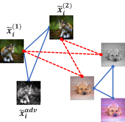
Figure 1: Prior works maximize the self-supervised contrastive loss between positive examples $\tilde{x}_{i}^{(1)},\tilde{x}_{i}^{(2)}$ when generating adversarial examples $\tilde{x}_{i}^{adv}$ (blue lines). In contrast, SwARo maximizes the loss for positive pairs (blue lines) but also creates targeted attacks by minimizing the loss for negative pairs (red lines).

Nevertheless, most instance-wise and cluster-based methods presented lack robustness to adversarial examples. A few works target improving robustness in contrastive learning by devising adversarial perturbations of positive and negative examples Kim et al. (2020); Jiang et al. (2020); McDermott et al. (2021); Bui et al. (2021). These efforts try to design adversarially robust self-supervised learning frameworks by generating perturbations that maximize the contrastive loss of augmented instance-level samples, causing the model to make incorrect predictions. However, semantic cluster structures encoded in the data are rarely considered, and the designed perturbations may not generalize well in downstream tasks. Intuitively, and in the absence of label (class) information, the self-supervised gradient-based adversarial attacks imposed can be considered untargeted, as the gradient points towards a direction that maximizes the contrastive loss for same-class instances, without any target class in mind (see Figure 1 blue lines).

In this work, we introduce Swapping Assignments for Robust contrastive learning (SwARo), a simple and efficient alternative that leverages cluster-wise supervision to design semi-targeted adversarial attacks that missguide the contrastive loss towards true negatives, i.e., accounting for examples that have pseudo-label assignments different than the anchor class. Specifically, our method updates the gradient direction to obtain adversarial perturbations that maximize the loss for pairs with same pseudo-labels (Figure 1 blue lines), but also minimize the loss of negative pairs (Figure 1 red lines), leading to pseudo-targeted attacks.

Contributions The contributions of our work are summarized as follows:

(1) We introduce SwARo, a self-supervised contrastive learning method that jointly considers adversarial robustness and cluster-wise semantic information observed in the data.

(2) In contrast to prior work on adversarial contrastive learning, we utilize the pseudo-labels induced by clustering as targets to explicitly guide the gradient direction towards negatives.

(3) We verify the effectiveness of the proposed method and show that SwARo improves downstream performance (accuracy), robustness on unseen black-box and white-box attack types, and transfer learning performance.

2 Related Work

Adversarial Training

There has been substantial research on increasing the robustness of deep neural networks against adversarial attacks. For example, Goodfellow et al. (2014) propose the Fast Gradient Sign Method (FGSM), a white-box attack that generates adversarial perturbations by utilizing the model gradients to design small distortions, which when added to the original image will lead to maximizing the model loss. Training with such adversarial perturbations has been shown to improve model robustness. Subsequent work proposes iterative variants, e.g., extensions such as the Basic Iterative (BIM) Kurakin et al. (2017) and Projected Gradient Descent (PGD) Madry et al. (2018) methods. Besides the gradient-based cross-entropy attacks, TRADES Zhang et al. (2019) empirically analyzes the trade-off between robustness and accuracy and introduces a defense mechanism that utilizes a KL-divergence loss between a clean example and its adversarial counterpart for learning a more robust latent feature space. Ilyas et al. (2019) hypothesize that the adversarial vulnerability of neural networks is a direct result of their sensitivity to well-generalizing features that are incomprehensible to humans. Schwinn et al. (2021) discover that cross-entropy attacks fail against models with large logits, and propose to add logit noise and enforce scale invariance on the loss to mitigate this limitation and encourage the model to design diverse attack targets. All above methods are originally designed for supervised learning tasks.

Contrastive Learning

Instance-wise contrastive learning methods Ye et al. (2019); Chen et al. (2020c); Bachman et al. (2019); He et al. (2020); Oord et al. (2018); Caron et al. (2021) learn an embedding space where different views of the same instance lie close to each other and views of dissimilar instances are pushed further away. For example, SimCLR Chen et al. (2020c) incorporates various data augmentation techniques to generate positive examples for contrastive training. MoCo He et al. (2020) utilizes a dynamic memory bank and a moving average encoder for calculating the contrastive loss. He et al. (2020) experiment with the number of negative examples and found that using more negatives results in learning better feature representations. However, due to only considering different views of the same instance as positive samples, instance-wise contrastive learning can not learn representations that capture the global class-level semantic structure of the training data. To alleviate this problem, clustering-based or prototypical contrastive learning Sharma et al. (2020); Li et al. (2020); Goyal et al. (2021) and supervised contrastive learning Khosla et al. (2020) methods have been proposed. For example, Li et al. (2020) utilize a cluster-based approach that brings contrastive representations closer to their assigned feature prototypes. Caron et al. (2020) propose SwAV, an image representation technique that instead of comparing representations of different image views, follows a swapped prediction strategy to predict the code of one view from another view of the same image by clustering image representations with a computationally efficient online clustering approach. Similar swapping strategies have been utilized in cross-modal retrieval Kim (2021). SEER Goyal et al. (2021) is trained on large-scale unconstrained and uncurated image collections by improving the scalability of SwAV in terms of GPU memory consumption and training speed. Khosla et al. (2020) extend contrastive learning to a supervised setting that utilizes label information in positive-negative subset creation, i.e., images of the same class label are considered as positive examples. All aforementioned instance-wise and cluster-based contrastive learning techniques lack robustness against adversarial examples. Here, we briefly review works that aim to combine adversarial training with contrastive learning.

Adversarial Contrastive Training

A number of works utilize adversarially constructed samples in contrastive learning to increase the robustness of the learned feature representations  Bui et al. (2021); Kim et al. (2020); Jiang et al. (2020); Chen et al. (2020b); McDermott et al. (2021); Chen et al. (2020a). RoCL Kim et al. (2020) introduces small perturbations to generate adversarial samples, leading to a more robust contrastive model. Jiang et al. (2020) experiment with different combinations of perturbations while generating positive and negative examples for calculating contrastive loss and found that using both standard data augmentations and adversarial samples increases robustness in a self-supervised pre-training procedure. Both works do not consider clustered prototypes during the contrastive loss computation or the adversarial sample generation process. Chen et al. (2020b) analyze robustness gains after applying adversarial training in both self-supervised pre-training and supervised fine-tuning, and find that adversarial pre-training contributes the most in robustness improvements. Bui et al. (2021) propose a minimax local-global algorithm to generate adversarial samples that improves the performance of SimCLR Chen et al. (2020c). To the best of our knowledge, none of the previous works considered designing more targeted contrastive adversarial examples by leveraging useful cluster structures observed in the data.

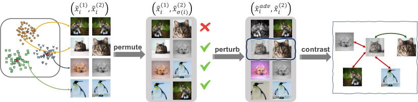
Figure 2: Pictorial overview of our proposed adversarial contrastive learning method SwARo. First, examples are pseudo-labeled via clustering and positive pairs are created by applying data augmentations to each example. Then, pairs are permuted to produce targets for the adversarial attack, that is guided by the pseudo-labels based on whether the permuted pair contains images from the same cluster or not. This process generates adversarial examples that are finally matched with their corresponding original pair examples to compute the contrastive loss. Inspired by targeted attacks, SwARo minimizes the loss for negative pairs and maximizes the loss for positive pairs. In contrast prior works only maximize the self-supervised contrastive loss between positive examples.

3 Proposed Method

Problem Formulation

Given a set of unlabeled instances $\mathcal{X}=\{x_{1},x_{2},...,x_{n}\}$, the goal is to learn a feature encoder $f_{\theta}(\cdot)\colon\mathcal{X}\to\mathbb{R}^{d}$ that maps data points to a $d$-dimensional embedding space and can later on be used in downstream tasks. Contrastive learning methods learn such feature representations by minimizing the distance between similar data points (positive pairs) and maximizing the distance between dissimilar data points (negative pairs). The contrastive loss is typically calculated via a normalized temperature-scaled cross-entropy loss (NT-XENT) as shown in Eq. (1).

$$\mathcal{L}_{CL}(x_{i},x_{k})\,{=}\,-\log\frac{\exp\big{(}s(x_{i},x_{k})/\tau\big{)}}{\sum\limits_{{x}_{j{\neq}i,k}\in\mathcal{X}}\exp\big{(}s(x_{i},x_{j})/\tau\big{)}},$$ (1)

where $s(x_{i},x_{j})\,{=}\,f_{\theta}(x_{i})^{\top}f_{\theta}(x_{j})/\lVert f_{\theta}(x_{i})\rVert\lVert f_{\theta}(x_{j})\rVert$ is the cosine similarity between two latent representations, $\tau$ is a temperature parameter, and $(x_{i},x_{k})$ is the positive pair while all other instances ${x}_{j{\neq}i,k}\in\mathcal{X}$ are considered negative pairs. The final contrastive loss is averaged across all positive pairs in a batch of examples.

It has been shown, however, that such formulations of contrastive learning are vulnerable against adversarial attacks Kim et al. (2020). Subsequently, a few adversarial self-supervised methods have been proposed that mainly apply adversarial training to contrastive pretraining such that the feature encoder $f_{\theta}$ learns robust data representations Kim et al. (2020); Jiang et al. (2020).

Supervised & Self-supervised Adversarial Training

In a supervised setting, adversarial training methods search for the worst-case instance perturbation that maximizes the supervised loss. To ensure that the semantic content of the instance does not alter, the perturbation space is constrained within a certain radius (e.g., $\ell_{\infty}$ norm-ball of radius $\epsilon$). The training objective is the following mini-max optimization problem:

$$\operatorname*{arg\,min}_{\theta}\mathbb{E}_{{(x_{i},y_{i})}\sim\mathcal{D}}\left[\max_{\|\delta_{i}\|_{\infty}\leq\epsilon}\mathcal{L}_{CE}(x_{i}+\delta_{i},y_{i};\theta)\right],$$ (2)

where $f_{\theta}\colon\mathcal{X}\to\mathcal{Y}$ denotes the supervised learning model with $\theta$ model parameters, $\mathcal{L}_{CE}$ is the supervised training objective, e.g., cross-entropy loss, and $(x_{i},y_{i})\in\mathcal{D}$ denotes a training sample with feature $x_{i}\in\mathcal{X}$ and corresponding label $y_{i}\in\mathcal{Y}$. Here, $\delta_{i}$ is the adversarial perturbation and subsequently $x_{i}+\delta_{i}$ is an adversarial example. There have been several gradient-based methods proposed to solve the inner maximization problem, essentially adjusting $\delta_{i}$ in the direction that maximizes the gradient $\nabla_{\delta_{i}}\mathcal{L}_{CE}(f_{\theta}(x_{i}+\delta_{i}),y_{i})$ Goodfellow et al. (2014); Kurakin et al. (2017); Madry et al. (2018); Zhang et al. (2019); Croce and Hein (2020); Schwinn et al. (2021). For example, the Projected Gradient Descent (PGD) Madry et al. (2018) iterates over gradient steps and adjusts $\delta$ accordingly:

$$\delta_{i}^{t+1}:=\Pi\Big{[}\delta_{i}^{t}+\eta\texttt{sign}\left(\nabla_{\delta_{i}}\mathcal{L}_{CE}\left(f_{\theta}(x_{i}+\delta_{i}^{t}),y_{i}\right)\right)\Big{]},$$ (3)

where $t$ denotes the number of iterations, $\eta$ is the step size, $\texttt{sign}(\cdot)$ is the vector sign (direction), and $\Pi$ denotes the norm-ball projection of interest, e.g., clipping $\delta_{i}$ to lie within an $\epsilon$-range $\Delta:=\{\delta\colon\|\delta_{i}\|_{\infty}\leq\epsilon\}$. Notice that the above formulation requires a class label $y\in\mathcal{Y}$ to compute the supervised loss when crafting adversarial attacks and hence is inapplicable to self-supervised settings. Also, depending on the choice of $y$, the attack can be untargeted or targeted. In targeted adversarial attacks the goal is to direct the perturbation towards a particular class of interest, other than the true class, e.g., confusing the model to misclassify a “cat” example as “dog”, by using as target $y$ the class label for “dog” instead of the model prediction.

To adapt adversarial training in self-supervised settings, recent work replaces the supervised loss with the contrastive NT-XENT loss in Eq.(1), i.e., generating adversarial views of an instance that confuse the model w.r.t. the instance identify (semantic class). However, this straightforward application of adversarial training can be considered as an untargeted attack that lacks the discriminative ability that observed data cluster structure (class) information can provide. In the following section, we present our proposed adversarial contrastive training approach.

3.1 SwARo Description

Our proposed adversarial contrastive method consists of three steps. At first, we assign each training sample into clusters via clustering. The choice of the clustering method is orthogonal to our approach. Then, we generate adversarial samples by perturbing the instances in each example pair, and guide the gradient for each example pair towards a corrected direction, based on whether the cluster assignments (pseudo-label) for the two instances are similar (and hence the two examples are most likely to encode a positive pair) or not (and this can be indeed considered as a negative pair). Afterward, we calculate the contrastive loss and update the encoder model. Each step is discussed in detail.

Cluster Assignments

We utilize clustering to obtain cluster centroids and assign a pseudo-label to each training sample. For simplicity, we apply $k$-means, however, we note that any clustering method can be used, including online clustering variants Asano et al. (2019); Caron et al. (2018, 2020). More formally, let $\mathcal{Z}\,{=}\,\{z_{1},z_{2},...,z_{n}\}$ be the intermediate latent representations obtained from feature encoder $f_{\theta}$ for unlabeled dataset $\mathcal{X}$, and $K$ is the empirically-set number of clusters. A set of cluster centroids $\mathcal{C}\,{=}\,\{c_{j}\}_{j=1}^{K}$ can be computed by applying $k$-means clustering on $\mathcal{Z}$. Next, we assign pseudo-label $\hat{y}_{x_{i}}$ to each example $x_{i}\in\mathcal{X}$ based on the distance from each cluster centroid, i.e., $\hat{y}_{x_{i}}\,{=}\,\operatorname*{arg\,min}_{j}{{(z_{i}-c_{j})}^{2}}$.

Adversarial Sample Generation

Let $\mathcal{X}_{B}\,{=}\,\{x_{i}\}^{B}_{i=1}\subset\mathcal{X}$ sampled batch of size $B$. To construct positive pairs, an example is augmented twice by applying two transformations $t_{1},t_{2}\in\mathcal{\mathcal{T}}$ that create two different views $\tilde{x}_{i}^{(1)}\,{=}\,t_{1}(x_{i})$ and $\tilde{x}_{i}^{(2)}\,{=}\,t_{2}(x_{i})$ of the same instance, producing a batch of positive pairs $\{(\tilde{x}_{1}^{(1)},\tilde{x}_{1}^{(2)}),\ldots,(\tilde{x}_{i}^{(1)},\tilde{x}_{i}^{(2)}),\ldots,(\tilde{x}_{B}^{(1)},\tilde{x}_{B}^{(2)})\}$. Without loss of generality, a permutation induced from shuffling the second instance in each pair is denoted as:

$$\{(\tilde{x}_{1}^{(1)},\tilde{x}_{\sigma(1)}^{(2)}),\ldots,(\tilde{x}_{i}^{(1)},\tilde{x}_{\sigma(i)}^{(2)}),\ldots,(\tilde{x}_{B}^{(1)},\tilde{x}_{\sigma(B)}^{(2)})\},$$ (4)

where $\sigma(\cdot)\colon\{1,\ldots,B\}\to\{1,\ldots,B\}$ is a permutation. Based on the pseudo-labels created from clustering (Section 3.1), we can assign an indicator variable to each pair in the batch, according to whether both instances belong to the same cluster, i.e.,

$$\mathcal{I}{\left(\tilde{x}_{i}^{(1)},\tilde{x}_{\sigma(i)}^{(2)}\right)}\,{=}\,\left[\mathbbm{1}\left(\hat{y}_{\tilde{x}_{i}^{(1)}}\,{=}\,\hat{y}_{\tilde{x}_{\sigma(i)}^{(2)}}\right)-\mathbbm{1}\left(\hat{y}_{\tilde{x}_{i}^{(1)}}\,{\neq}\,\hat{y}_{\tilde{x}_{\sigma(i)}^{(2)}}\right)\right],$$ (5)

where $\hat{y}_{\tilde{x}_{i}^{(1)}}$ and $\hat{y}_{\tilde{x}_{\sigma(i)}^{(2)}}$ are pseudo-labels from clustering.

In short, we assign $\mathcal{I}{\left(\tilde{x}_{i}^{(1)},\tilde{x}_{\sigma(i)}^{(2)}\right)}=1$ to a pair if both of the examples in that pair belongs to the same cluster (positive pair) and $\mathcal{I}{\left(\tilde{x}_{i}^{(1)},\tilde{x}_{\sigma(i)}^{(2)}\right)}=-1$ if they belong to different clusters (negative pair). We utilize this indicator to better guide the sign of the NT-XENT gradient w.r.t. the corresponding example pair. In essence, we maximize the contrastive loss w.r.t. positive pairs, and minimize the contrastive loss w.r.t. negative pairs, as shown in Eq. (6):

$$\delta_{i}^{t+1}:=\Pi\left[\delta_{i}^{t}+\eta~{}{\beta}_{x_{i}}\texttt{sign}\left(\nabla_{\delta_{i}}\mathcal{L}_{CL}\left(f_{\theta}\left(\tilde{x_{i}}^{(1)}+\delta_{i}^{t}\right),~{}f_{\theta}\left(\tilde{x}_{\sigma(i)}^{(2)}\right)\right)\right)\right],$$ (6)

where ${\beta}_{x_{i}}\,{=}\,\mathcal{I}{\left(\tilde{x}_{i}^{(1)},\tilde{x}_{\sigma(i)}^{(2)}\right)}$ for brevity. Notice that $f_{\theta}\left(\tilde{x}_{\sigma(i)}^{(2)}\right)$, in combination with ${\beta}_{x_{i}}$, acts as a target for the adversarial attack. Applying these pertubations to each example in the batch creates adversarial examples $x^{adv}_{i}\,{=}\,\left(\tilde{x}_{i}^{(1)}+\delta_{i}^{(1)},\tilde{x}_{\sigma(i)}^{(2)}\right)$ that aim to maximize the similarity when both examples in a pair belong to different clusters.

Contrastive Training

Finally, pairs are reordered in their original configuration $\mathcal{X}^{adv}\,{=}\,\{(\tilde{x}_{i}^{(1)}+\delta_{i}^{(1)},~{}\tilde{x}_{i}^{(2)})\}_{i=1}^{B}$, with one instance in each pair being adversarially attacked, and the model is trained with the contrastive NT-XENT loss computed as in Eq.(1). Figure 2 presents an overview and Algorithm 1 provides the pseudocode of the proposed method.

Algorithm 1 Pseudocode for SwARo

  Input: Unlabeled dataset $\mathcal{X}$, batch size $B$, encoder $f_{\theta}$, transformations $\mathcal{\mathcal{T}}$

  for batch $\mathcal{X}_{B}\,{=}\,\{(x_{i})\}_{i=1}^{B}\subset\mathcal{X}$ do

     $\texttt{loss}:=0$, $\mathcal{S}\,{=}\,\emptyset$

     for $i=1,\ldots,B$ do   # Augment $x_{i}$ with transformations sampled from $\mathcal{\mathcal{T}}$

        $\tilde{x}_{i}^{(1)}\,{=}\,t_{1}(x_{i})$ and $\tilde{x}_{i}^{(2)}\,{=}\,t_{2}(x_{i})$

        $\mathcal{S}\,{=}\,\mathcal{S}\cup\left\{\left(\tilde{x}_{i}^{(1)},\tilde{x}_{i}^{(2)}\right)\right\}$ # collect pairs

     end for

     $\sigma(\mathcal{S})\,{=}\,\left\{\left(\tilde{x}_{i}^{(1)},\tilde{x}_{\sigma(i)}^{(2)}\right)\right\}_{i=1}^{B}$    # Permute instances

     for $i=1,\ldots,B$ do

        ${\beta}_{x_{i}}\,{=}\,\left[\mathbbm{1}\left(\hat{y}_{\tilde{x}_{i}^{(1)}}\,{=}\,\hat{y}_{\tilde{x}_{\sigma(i)}^{(2)}}\right)-\mathbbm{1}\left(\hat{y}_{\tilde{x}_{i}^{(1)}}\,{\neq}\,\hat{y}_{\tilde{x}_{\sigma(i)}^{(2)}}\right)\right]$    # Assign indicator to each pair via Eq.(5)

        for $t=1,\ldots,T$ do

             $\delta_{i}^{t+1}:=\Pi\left[\delta_{i}^{t}+\eta~{}{\beta}_{x_{i}}\texttt{sign}\left(\nabla_{\delta_{i}}\mathcal{L}_{CL}\left(f_{\theta}\left(\tilde{x_{i}}^{(1)}+\delta_{i}^{t}\right),~{}f_{\theta}\left(\tilde{x}_{\sigma(i)}^{(2)}\right)\right)\right)\right],$

            # Compute adversarial perturbations via Eq.(6)

        end for

        $x^{adv}_{i}\,{=}\,\left(\tilde{x}_{i}^{(1)}+\delta_{i}^{(1)},~{}\tilde{x}_{i}^{(2)}\right)$    # Apply adversarial permutation to original pair

        $\mathcal{S}\,{=}\,\mathcal{S}\setminus\left\{\left(\tilde{x}_{i}^{(1)},~{}\tilde{x}_{i}^{(2)}\right)\right\}\cup x^{adv}_{i}$ # Update $\mathcal{S}$

     end for

     loss += $\sum\limits_{i\in B}\left[-\log\frac{\exp\big{(}s\left(\tilde{x}_{i}^{(1)}+\delta_{i}^{(1)},\tilde{x}_{i}^{(2)}\right)/\tau\big{)}}{\sum\limits_{{x}_{j{\neq}i}\in\mathcal{X}}\exp\big{(}s\left(\tilde{x}_{i}^{(1)}+\delta_{i}^{(1)},\tilde{x}_{i}^{(2)}\right)/\tau\big{)}}\right]$    # calculate contrastive loss

     end for

     update model parameters $\theta$ to minimize the loss

  end for

4 Experimental Results

We evaluate SwARo on two benchmark datasets comparing against existing self-supervised and supervised adversarial learning methods, and reporting results on black-box and white-box targeted and untargeted attacks. Similarly to Kim et al. (2020), we consider a linear evaluation and a robust-linear evaluation (r-LE) setting, where we compare the classification accuracy on clean and adversarial examples, respectively.

Experimental Setup

For all experiments, we use a ResNet-18 He et al. (2016) as the backbone encoder. All models, including baselines are trained with $\ell_{\infty}$ Projected Gradient Descent (PGD) with $\epsilon=8/255$. As for the linear evaluation, we follow a similar setup as RoCL Kim et al. (2020), where we first train an unsupervised model and then train a linear layer to measure the accuracy. All reported results are averaged over multiple trials, and hyper-parameters are provided in the supplementary material. To ensure the efficacy of the clustering process, we rely on instance-wise adversarial attacks for the first 100 epochs and then utilize the proposed cluster-wise adversarial example generation. This is to guarantee that the encoder has learned useful representations before initiating clustering.

Datasets & Baselines

We conduct experiments on the following datasets:

CIFAR-10 (Krizhevsky et al., 2009): The CIFAR-10 dataset includes $60,000$ images of size $32\times 32$, originating from $10$ classes, with $6,000$ images per class. The training and test sets consist of $50,000$ and $10,000$ images, respectively.

CIFAR-100 (Krizhevsky et al., 2009) contains images similar to CIFAR-10 but there exist $100$ classes and $600$ images per class. Train-to-test ratio remains the same as CIFAR-10.

Moreover, we compare SwARo against six types of baseline methods: (1) Supervised models trained with cross-entropy (CE), (2) traditional adversarial training methods such as AT Madry et al. (2018) and TRADES Zhang et al. (2019), (3) a vanilla contrastive learning method, SimCLR Chen et al. (2020c), (4) supervised contrastive learning (SCL)  Khosla et al. (2020), (5) SwAV Caron et al. (2020), a contrastive method that utilizes clustering, and (6) adversarial contrastive learning methods such as RoCL Kim et al. (2020) and ACL Jiang et al. (2020).

Table 1: Comparison against PGD white-box attacks on CIFAR-10. Results marked with ^† are reported from  Kim et al. (2020). CE is supervised cross-entropy. $A_{nat}$ denotes the accuracy of clean images. $\ell_{\infty}$ is the seen adversarial attack while $\ell_{1}$ and $\ell_{2}$ are unseen attacks. Colored fonts indicate best performance in each category: supervised (violet), self-supervised (teal), adversarial self-supervised on linear evaluation (black), and robust linear evaluation (purple).

Train type	Method		seen		unseen
			$\ell_{\infty}$		$\ell_{2}$		$\ell_{1}$
		$A_{nat}$	$\epsilon$ 8/255	16/255	0.25	0.5	7.84	12
Supervised	CE†	92.82	0.00	0.00	20.77	12.96	28.47	15.56
	AT†  Madry et al. (2018)	81.63	44.50	14.47	72.26	59.26	66.74	55.74
	TRADES† Zhang et al. (2019)	77.03	48.01	22.55	68.07	57.93	62.93	53.79
	SCL† Khosla et al. (2020)	94.05	0.08	0.00	22.17	10.29	38.87	22.58
Self- supervised	SimCLR† Chen et al. (2020c)	91.25	0.63	0.08	15.3	2.08	41.49	25.76
	SwAV Caron et al. (2020)	70.60	22.88	18.46	35.54	35.53	35.54	35.54
Adversarial Self-supervised	RoCL† Kim et al. (2020)	83.71	40.27	9.55	66.39	63.82	79.21	76.17
	ACL Jiang et al. (2020)	80.91	41.39	12.95	75.00	75.45	79.32	79.30
	SwARo (Ours)	87.38	37.33	9.13	59.69	59.10	84.06	83.69
Adversarial (Robust Eval.) Self-supervised	RoCL+rLE†	80.43	47.69	15.53	68.30	66.19	77.31	75.05
	SwARo (Ours) + rLE	86.89	41.58	10.70	62.20	62.66	84.09	83.79

Table 2: Comparison against PGD white-box attacks on CIFAR-100. $A_{nat}$ denotes the accuracy of clean images. $\ell_{\infty}$ is the seen adversarial attack while $\ell_{1}$ and $\ell_{2}$ are unseen attacks.

Method		seen		unseen
		$\ell_{\infty}$		$\ell_{2}$		$\ell_{1}$
	$A_{nat}$	$\epsilon$ 8/255	16/255	0.25	0.5	7.84	12
ACL Jiang et al. (2020)	42.03	22.97	9.53	38.37	38.67	40.92	40.88
RoCL Kim et al. (2020)	50.04	20.26	5.93	36.16	36.09	52.44	52.08
SwARo (Ours)	55.12	20.19	5.96	36.37	36.11	52.44	52.18

4.1 White Box Attacks

We first evaluate the robustness of the learned representations against seen and unseen attacks. In Table 1, we report results on CIFAR-10, comparing methods against Projected Gradient Descent (PGD) white-box attacks with linear evaluation and robust linear evaluation (rLE).  Table 2 presents results for all adversarial self-supervised methods on CIFAR-100.

Traditional contrastive learning methods (SimCLR and SwAV) are vulnerable to adversarial attacks. Considering cluster information (SwAV) improves performance on seen $\ell_{\infty}$ attacks and unseen $\ell_{2}$ attacks but occurs considerable losses in accuracy on clean images $A_{nat}$. Among adversarial self-supervised approaches, SwARo achieves much higher clean accuracy, substantially higher robust accuracy against unseen $\ell_{1}$ target attacks, and comparable performance with RoCL on $\ell_{\infty}$ and $\ell_{2}$ attacks. ACL outperforms both on $\ell_{\infty}$ and $\ell_{2}$; this method benefits from additional batch normalization parameters and balancing two contrastive loss terms, a standard contrastive and an adversarial contrastive loss.

In addition to PGD, we also experiment with several additional state-of-the-art white-box attacks BIM Kurakin et al. (2017), FGSM Goodfellow et al. (2014), Jitter Schwinn et al. (2021). SwARo outperforms baselines across all untargeted and targeted white-box attacks, showing consistent robust accuracy gains (Table 3). In particular, we observe approximately $3-4\%$ relative gains on PDG variants such as BIM and FGSM w.r.t. the next best method. Additionally, we find that SwARo is performing $4-9\%$ better compared to baselines on Jitter attacks, an adversarial attack method that incorporates scale invariance and encourages diverse attack targets with smaller perturbations Schwinn et al. (2021). These results make SwARo more appealing in practice and suggest that our approach to enforcing adversarial perturbations, that consider both positive and negative pairs as well as semantic cluster information, ensures robustness against a diverse set of attack types.

Table 3: Performance of SwARo against white-box attacks (BIM, FGSM, Jitter) on the CIFAR-10 dataset. Each column denotes the white-box attack used to generate adversarial samples with $\epsilon=$8/255. Each row shows the performance of the target models against the white-box attacks.

	BIM Kurakin et al. (2017)		FGSM Goodfellow et al. (2014)		Jitter Schwinn et al. (2021)
	Untargeted	Targeted	Untargeted	Targeted	Untargeted	Targeted
RoCL	37.07	62.92	57.27	67.06	45.41	63.67
ACL	42.35	65.74	49.95	63.02	54.24	61.55
SwARo (Ours)	45.78↑3.43	68.70↑2.96	61.34↑4.07	67.83↑0.77	57.75↑3.51	72.57↑8.90

Table 4: Performance comparison against black-box attacks on the CIFAR-10 dataset. Columns denote black-box $\ell_{\infty}$ attacks and rows show model performance (models trained with $\ell_{\infty}$).

	$\epsilon=$8/255				$\epsilon=$16/255
	AT	TRADES	RoCL	SwARo	AT	TRADES	RoCL	SwARo
AT Madry et al. (2018)	-	41.67$\pm$0.06	43.06$\pm$0.08	43.53$\pm$0.05	-	36.97$\pm$0.08	40.81$\pm$0.14	41.89$\pm$0.06
TRADES Zhang et al. (2019)	82.29$\pm$0.04	-	74.43$\pm$0.04	73.31$\pm$0.10	80.10$\pm$0.09	-	55.88$\pm$0.11	55.55$\pm$0.07
RoCL Kim et al. (2020)	82.03$\pm$0.07	71.39$\pm$0.02	-	61.41$\pm$0.08	79.11$\pm$0.08	46.09$\pm$0.10	-	28.86$\pm$0.15
ACL Jiang et al. (2020)	80.28$\pm$0.05	69.62$\pm$0.04	63.53$\pm$0.04	63.06$\pm$0.10	77.93$\pm$0.13	45.56$\pm$0.03	32.48$\pm$0.07	33.33$\pm$0.14
SwARo (Ours)	84.99$\pm$0.12	74.38$\pm$0.08	64.27$\pm$0.12	-	81.80$\pm$0.23	45.40$\pm$0.09	25.61$\pm$0.15	-

4.2 Black Box Attacks

We also verify the performance of SwARo against black-box attacks. We generate adversarial examples using black-box $\ell_{\infty}$ attacks such as AT Madry et al. (2018)) and TRADES Zhang et al. (2019). Table 4 shows that SwARo is able to better defend against TRADES and AT attacks. We additionally compare SwARo as a black-box adversarial attack on TRADES, AT, RoCL and ACL. Results show that SwARo attacks are stronger or comparable to baselines. An interesting observation is that as the perturbation radius $\epsilon$ becomes smaller, SwARo as an attack is stronger than RoCL, as SwARo’s performance on RoCL attacks is $64.27\%$, compared to RoCL’s performance on SwARo attacks that drops to $61.41\%$. Similarly, we also find that ACL and TRADES are better equipped against RoCL attacks than SwARo attacks.

4.3 Transfer Learning

We evaluate performance on a transfer learning setup and check whether the learned representations can be transferred across datasets. Specifically, we pretrain an encoder model on CIFAR-10 and then finetune a randomly-initialized linear classification layer on CIFAR-100, on top of the frozen encoder. We compare against adversarial self-supervised baselines, ACL Jiang et al. (2020) and ROCL Kim et al. (2020). As shown in Table 5, SwARo achieves better accuracy across all cases.

Table 5: Comparison in a transfer learning setup across the CIFAR-10 and CIFAR-100 datasets with ResNet-18. Column “Source” corresponds to the dataset the encoder model is trained on, while “Target” presents the dataset used for evaluating the frozen encoder with an additional randomly-initialized finetuned linear layer (linear evaluation).

Model	Source	Target	$A_{nat}$	Source	Target	$A_{nat}$
ACL Jiang et al. (2020)	CIFAR-100	CIFAR-10	70.08	CIFAR-10	CIFAR-100	42.29
RoCL Kim et al. (2020)			73.93			45.84
SwARo (Ours)			75.52			46.01

4.4 Ablation Studies

We study the trade-off between robustness and accuracy. In particular, we design an ablation study among our proposed SwARo and a stochastic variant that selects between the targeted attacks and the traditional adversarial contrastive learning that maximizes the loss between positive pairs. Since our method improves accuracy on clean images and on unseen $\ell_{1}$ attacks, we hope that this stochastic selection will be able to balance between this improvement and robustness to seen attacks. In Table 6, the first column $p$ presents the probability of selecting an adversarial generation strategy. For example, $p=0.90$ denotes applying the proposed SwARo adversarial contrastive method to $90\%$ of the batches during training, while applying RoCL to $10\%$ of the batches. Results show that smaller $p$ values result in improvements on seen $\ell_{\infty}$ attacks and unseen $\ell_{2}$ attacks, while the performance on clean images and unseen $\ell_{1}$ attacks improves as $p$ increases. We leave further exploration with other stochastic variants and extensive hyper-parameter tuning to future work. We perform additional ablation studies to test the effect of clustering and the variability on performance as training progresses. Results can be found in the supplementary material.

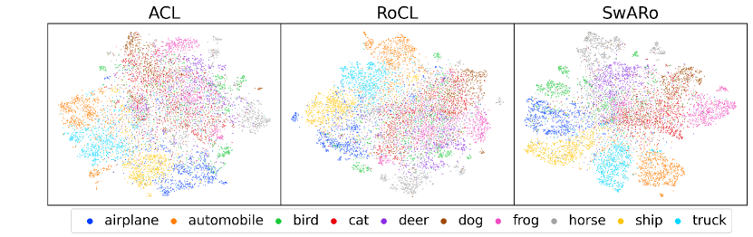
Figure 3: t-SNE visualization of the three contrastive pretraining methods ACL Jiang et al. (2020), RoCL Kim et al. (2020) and SwARo (Ours) on the CIFAR-10 dataset. The 10 classes are represented with different colors, and the legend shows label information. SwARo produces well-separated clusters compared to the rest of the baselines.

Table 6: Performance of SwARo, varying the probability of selection $p$ for the proposed adversarial example generation or reverting to the traditional contrastive adversarial example generation Kim et al. (2020). Results reported on the CIFAR-10 dataset.

p		seen		unseen
		$\ell_{\infty}$		$\ell_{2}$		$\ell_{1}$
	$A_{nat}$	$\epsilon$ 8/255	16/255	0.25	0.5	7.84	12
0.10	84.11	39.58	10.68	73.80	72.51	82.31	82.25
0.25	84.11	37.93	9.26	73.09	70.36	82.04	81.92
0.50	85.78	38.37	10.10	68.78	67.76	83.30	82.70
0.75	87.38	37.33	9.13	59.69	59.10	84.06	83.69
0.90	89.13	35.95	9.68	42.02	47.86	84.98	84.36

4.5 Qualitative Analysis

We present qualitative results on the learned representations. We create t-SNE visualizations Van der Maaten and Hinton (2008) for RoCL, ACL and our method SwARo. Each semantic class on the CIFAR-10 dataset is assigned a different color, and the legend presents the object category. Figure 3 shows that representations obtained from SwARo produce well-separated clusters compared to the baselines. Overall our results indicate that SwARo results in better representation learning performance and improved robustness to unseen attacks.

5 Conclusion

In this work, we present SwARo, an adversarial contrastive learning method that learns robust self-supervised representations. Our approach is able to better guide the adversarial perturbation process. More specifically, by permuting pseudo-labels our method is able to create targeted attacks that maximize the loss for positive pairs and minimize the loss for negative pairs, leading to improvements in clean accuracy and unseen attacks. Through experimental analysis on black-box and white-box attacks, with two benchmark datasets and comparing against a variety of baselines, ranging from vanilla self-supervised methods to previously proposed adversarial contrastive learning approaches, we showcase that our proposed approach, SwARo, outperforms baselines that only consider positive pairs when creating adversarial examples. Additional experiments on a diverse set of white-box attacks show that SwARo is robust on realistic adversarial scenarios against a diverse set of attack types. Qualitative analysis shows that incorporating pseudo-label information produces well-separated clusters, leading to better learned robust representations. In the future, we hope to evaluate our method on additional datasets with more complex model architectures. Future directions could include extensions to multi-modal data and structured tasks, as well as improving robustness on hierarchical fine-grained representation learning settings.

Appendix A Appendix

A.1 Training Progress

In addition, we present the learning progress as the number of epochs increases. Table 7 reports results on CIFAR-10, on both clean accuracy and robust accuracy on seen and unseen attacks.

Table 7: Ablation study on the number of epochs. Results reported on the CIFAR-10 dataset.

Number of Epochs		seen		unseen
		$\ell_{\infty}$		$\ell_{2}$		$\ell_{1}$
	$A_{nat}$	$\epsilon$ 8/255	16/255	0.25	0.5	7.84	12
200	78.03	27.73	6.44	51.96	51.66	78.14	77.64
400	81.97	23.90	4.69	51.87	50.90	73.46	72.99
600	83.32	29.79	6.31	54.82	53.20	79.85	79.34
800	85.63	32.04	6.51	59.78	58.90	81.67	81.25
1000	84.43	33.03	7.52	57.65	57.20	82.52	81.99
1200	86.55	33.91	7.92	61.13	59.92	83.44	82.98
1400	87.05	36.53	9.13	59.38	59.35	83.97	83.57
1600	87.21	36.32	8.62	60.66	60.50	84.23	83.82
1800	87.35	36.94	8.80	58.81	59.21	84.09	83.69
2000	87.38	37.33	9.13	59.69	59.10	84.06	83.69

A.2 Number of Clusters

Table 8 presents results with varying the number of clusters $K$. In general, there are marginal performance differences across clean and robust accuracy, and seen and unseen attacks, showing that SwARo remains robust to the choice of this hyper-parameter.

Table 8: Ablation study on the number of clusters. Results reported on the CIFAR-10 dataset.

#$K$ Clusters		seen		unseen
		$\ell_{\infty}$		$\ell_{2}$		$\ell_{1}$
	$A_{nat}$	$\epsilon$ 8/255	16/255	0.25	0.5	7.84	12
25	87.61	37.34	9.49	59.07	59.91	84.36	84.10
50	87.12	37.86	9.48	57.98	60.72	84.60	84.21
100	87.42	37.36	9.61	58.91	59.41	84.21	83.79
250	87.79	37.72	9.17	59.22	61.21	85.26	84.84
500	87.42	36.98	9.26	59.12	59.44	84.37	83.81
1000	87.38	37.33	9.13	59.69	59.10	84.06	83.69
2500	87.38	37.83	8.96	58.68	59.90	84.57	84.08
5000	87.34	37.35	9.67	59.26	59.41	84.44	83.95
10000	87.48	38.17	9.01	56.46	59.91	84.37	83.70

A.3 Hyper-parameter Details

For all models, we adopt the training setup of RoCL Kim et al. [2020]. For completeness, in this supplementary material we report important hyper-parameters, as well as newly introduced hyper-parameters. We use a $0.01$ learning rate for linear evaluation and $0.02$ for robust linear evaluation. We utilize a ResNet-18 as a base encoder for all models. In the training phase, we use a two-layered projection layer as the projection head. The embedding dimension of the projection head is 128. For the adversarial attacks in the training phase, we set $\epsilon=8/255$ and $\eta=1/255$, and $t=7$. Here $\epsilon$ is the perturbation radius, $\eta$ is the step size, and $t$ is the number of PGD iterations. Unless otherwise specified, we use $K=1000$ for CIFAR-10 and $K=5000$ for CIFAR-100, where $K$ is the number of clusters. We set $p=0.75$, which is the probability of applying SwARo to a batch. We train all our models for $2000$ epochs. We use a batch size of $256$ for running all our training. For the rest, we follow a similar optimization setup and data augmentation as RoCL Kim et al. [2020]. Training time for SwARo is approximately 5 hours and 20 minutes per 100 epochs with two NVIDIA V100 GPUs with 16GB memory.

References

- Alwassel et al. [2020] Humam Alwassel, Dhruv Mahajan, Bruno Korbar, Lorenzo Torresani, Bernard Ghanem, and Du Tran. Self-supervised learning by cross-modal audio-video clustering. In Advances in Neural Information Processing Systems (NeurIPS), 2020.
- Asano et al. [2019] YM Asano, C Rupprecht, and A Vedaldi. Self-labelling via simultaneous clustering and representation learning. In International Conference on Learning Representations (ICLR), 2019.
- Bachman et al. [2019] Philip Bachman, R Devon Hjelm, and William Buchwalter. Learning representations by maximizing mutual information across views. In Advances in Neural Information Processing Systems (NeurIPS), 2019.
- Bui et al. [2021] Anh Bui, Trung Le, He Zhao, Paul Montague, Seyit Camtepe, and Dinh Phung. Understanding and achieving efficient robustness with adversarial contrastive learning. arXiv preprint arXiv:2101.10027, 2021.
- Caron et al. [2018] Mathilde Caron, Piotr Bojanowski, Armand Joulin, and Matthijs Douze. Deep clustering for unsupervised learning of visual features. In European Conference on Computer Vision (ECCV), 2018.
- Caron et al. [2020] Mathilde Caron, Ishan Misra, Julien Mairal, Priya Goyal, Piotr Bojanowski, and Armand Joulin. Unsupervised learning of visual features by contrasting cluster assignments. In Advances in Neural Information Processing Systems (NeurIPS), 2020.
- Caron et al. [2021] Mathilde Caron, Hugo Touvron, Ishan Misra, Hervé Jégou, Julien Mairal, Piotr Bojanowski, and Armand Joulin. Emerging properties in self-supervised vision transformers. arXiv preprint arXiv:2104.14294, 2021.
- Chen et al. [2020a] Kejiang Chen, Yuefeng Chen, Hang Zhou, Xiaofeng Mao, Yuhong Li, Yuan He, Hui Xue, Weiming Zhang, and Nenghai Yu. Self-supervised adversarial training. In IEEE International Conference on Acoustics, Speech and Signal Processing (ICASSP), 2020a.
- Chen et al. [2020b] Tianlong Chen, Sijia Liu, Shiyu Chang, Yu Cheng, Lisa Amini, and Zhangyang Wang. Adversarial robustness: From self-supervised pre-training to fine-tuning. In IEEE/CVF Conference on Computer Vision and Pattern Recognition (CVPR), 2020b.
- Chen et al. [2020c] Ting Chen, Simon Kornblith, Mohammad Norouzi, and Geoffrey Hinton. A simple framework for contrastive learning of visual representations. In International Conference on Machine Learning (ICML), 2020c.
- Chen et al. [2020d] Xinlei Chen, Haoqi Fan, Ross Girshick, and Kaiming He. Improved baselines with momentum contrastive learning. arXiv preprint arXiv:2003.04297, 2020d.
- Chuang et al. [2020] Ching-Yao Chuang, Joshua Robinson, Lin Yen-Chen, Antonio Torralba, and Stefanie Jegelka. Debiased contrastive learning. In Advances in Neural Information Processing Systems (NeurIPS), 2020.
- Croce and Hein [2020] Francesco Croce and Matthias Hein. Reliable evaluation of adversarial robustness with an ensemble of diverse parameter-free attacks. In International Conference on Machine Learning (ICML), 2020.
- Goodfellow et al. [2014] Ian J Goodfellow, Jonathon Shlens, and Christian Szegedy. Explaining and harnessing adversarial examples. arXiv preprint arXiv:1412.6572, 2014.
- Goyal et al. [2021] Priya Goyal, Mathilde Caron, Benjamin Lefaudeux, Min Xu, Pengchao Wang, Vivek Pai, Mannat Singh, Vitaliy Liptchinsky, Ishan Misra, Armand Joulin, et al. Self-supervised pretraining of visual features in the wild. arXiv preprint arXiv:2103.01988, 2021.
- Han et al. [2019] Kai Han, Andrea Vedaldi, and Andrew Zisserman. Learning to discover novel visual categories via deep transfer clustering. In IEEE/CVF Conference on Computer Vision and Pattern Recognition (CVPR), 2019.
- He et al. [2016] Kaiming He, Xiangyu Zhang, Shaoqing Ren, and Jian Sun. Deep residual learning for image recognition. In IEEE/CVF Conference on Computer Vision and Pattern Recognition (CVPR), 2016.
- He et al. [2020] Kaiming He, Haoqi Fan, Yuxin Wu, Saining Xie, and Ross Girshick. Momentum contrast for unsupervised visual representation learning. In IEEE/CVF Conference on Computer Vision and Pattern Recognition (CVPR), 2020.
- Henaff [2020] Olivier Henaff. Data-efficient image recognition with contrastive predictive coding. In International Conference on Machine Learning (ICML), 2020.
- Hjelm et al. [2018] R Devon Hjelm, Alex Fedorov, Samuel Lavoie-Marchildon, Karan Grewal, Phil Bachman, Adam Trischler, and Yoshua Bengio. Learning deep representations by mutual information estimation and maximization. In International Conference on Learning Representations (ICLR), 2018.
- Hu et al. [2021] Peng Hu, Xi Peng, Hongyuan Zhu, Liangli Zhen, and Jie Lin. Learning cross-modal retrieval with noisy labels. In IEEE/CVF Conference on Computer Vision and Pattern Recognition (CVPR), 2021.
- Ilyas et al. [2019] Andrew Ilyas, Shibani Santurkar, Dimitris Tsipras, Logan Engstrom, Brandon Tran, and Aleksander Madry. Adversarial examples are not bugs, they are features. arXiv preprint arXiv:1905.02175, 2019.
- Jiang et al. [2020] Ziyu Jiang, Tianlong Chen, Ting Chen, and Zhangyang Wang. Robust pre-training by adversarial contrastive learning. In Advances in Neural Information Processing Systems (NeurIPS), 2020.
- Khosla et al. [2020] Prannay Khosla, Piotr Teterwak, Chen Wang, Aaron Sarna, Yonglong Tian, Phillip Isola, Aaron Maschinot, Ce Liu, and Dilip Krishnan. Supervised contrastive learning. In Advances in Neural Information Processing Systems (NeurIPS), 2020.
- Kim et al. [2020] Minseon Kim, Jihoon Tack, and Sung Ju Hwang. Adversarial self-supervised contrastive learning. In Advances in Neural Information Processing Systems (NeurIPS), 2020.
- Kim [2021] Minyoung Kim. Swamp: Swapped assignment of multi-modal pairs for cross-modal retrieval. arXiv preprint arXiv:2111.05814, 2021.
- Krizhevsky et al. [2009] Alex Krizhevsky, Vinod Nair, and Geoffrey Hinton. Cifar-10/cifar100 (canadian institute for advanced research). 2009.
- Kuo et al. [2020] Chia-Wen Kuo, Chih-Yao Ma, Jia-Bin Huang, and Zsolt Kira. Featmatch: Feature-based augmentation for semi-supervised learning. In European Conference on Computer Vision (ECCV), 2020.
- Kurakin et al. [2017] Alexey Kurakin, Ian J. Goodfellow, and Samy Bengio. Adversarial examples in the physical world. ArXiv, abs/1607.02533, 2017.
- Li et al. [2021] Jichang Li, Guanbin Li, Yemin Shi, and Yizhou Yu. Cross-domain adaptive clustering for semi-supervised domain adaptation. In IEEE/CVF Conference on Computer Vision and Pattern Recognition (CVPR), 2021.
- Li et al. [2020] Junnan Li, Pan Zhou, Caiming Xiong, and Steven Hoi. Prototypical contrastive learning of unsupervised representations. In International Conference on Learning Representations (ICLR), 2020.
- Madry et al. [2018] Aleksander Madry, Aleksandar Makelov, Ludwig Schmidt, Dimitris Tsipras, and Adrian Vladu. Towards deep learning models resistant to adversarial attacks. In International Conference on Learning Representations (ICLR), 2018.
- McDermott et al. [2021] Matthew McDermott, Brendan Yap, Harry Hsu, Di Jin, and Peter Szolovits. Adversarial contrastive pre-training for protein sequences. arXiv preprint arXiv:2102.00466, 2021.
- Oord et al. [2018] Aaron van den Oord, Yazhe Li, and Oriol Vinyals. Representation learning with contrastive predictive coding. arXiv preprint arXiv:1807.03748, 2018.
- Robinson et al. [2021] Joshua Robinson, Ching-Yao Chuang, Suvrit Sra, and Stefanie Jegelka. Contrastive learning with hard negative samples. In International Conference on Learning Representations (ICLR), 2021.
- Schwinn et al. [2021] Leo Schwinn, René Raab, An Nguyen, Dario Zanca, and Bjoern Eskofier. Exploring misclassifications of robust neural networks to enhance adversarial attacks. arXiv preprint arXiv:2105.10304, 2021.
- Sharma et al. [2020] Vivek Sharma, Makarand Tapaswi, M Saquib Sarfraz, and Rainer Stiefelhagen. Clustering based contrastive learning for improving face representations. In IEEE International Conference on Automatic Face and Gesture Recognition, 2020.
- Tian et al. [2019] Yonglong Tian, Dilip Krishnan, and Phillip Isola. Contrastive multiview coding. In European Conference on Computer Vision (ECCV), 2019.
- Van der Maaten and Hinton [2008] Laurens Van der Maaten and Geoffrey Hinton. Visualizing data using t-sne. Journal of machine learning research, 2008.
- Yang et al. [2021] Jingkang Yang, Haoqi Wang, Litong Feng, Xiaopeng Yan, Huabin Zheng, Wayne Zhang, and Ziwei Liu. Semantically coherent out-of-distribution detection. In IEEE/CVF Conference on Computer Vision and Pattern Recognition (CVPR), 2021.
- Ye et al. [2019] Mang Ye, Xu Zhang, Pong C Yuen, and Shih-Fu Chang. Unsupervised embedding learning via invariant and spreading instance feature. In IEEE/CVF Conference on Computer Vision and Pattern Recognition (CVPR), 2019.
- Zhang et al. [2019] Hongyang Zhang, Yaodong Yu, Jiantao Jiao, Eric Xing, Laurent El Ghaoui, and Michael Jordan. Theoretically principled trade-off between robustness and accuracy. In International Conference on Machine Learning (ICLR), 2019.
- Zhang et al. [2009] Kai Zhang, James T Kwok, and Bahram Parvin. Prototype vector machine for large scale semi-supervised learning. In International Conference on Machine Learning (ICML), 2009.