Share With Thy Neighbors: Single-View Reconstruction by Cross-Instance Consistency

Abstract

Approaches for single-view reconstruction typically rely on viewpoint annotations, silhouettes, the absence of background, multiple views of the same instance, a template shape, or symmetry. We avoid all such supervision and assumptions by explicitly leveraging the consistency between images of different object instances. As a result, our method can learn from large collections of unlabelled images depicting the same object category. Our main contributions are two ways for leveraging cross-instance consistency: (i) progressive conditioning, a training strategy to gradually specialize the model from category to instances in a curriculum learning fashion; and (ii) neighbor reconstruction, a loss enforcing consistency between instances having similar shape or texture. Also critical to the success of our method are: our structured autoencoding architecture decomposing an image into explicit shape, texture, pose, and background; an adapted formulation of differential rendering; and a new optimization scheme alternating between 3D and pose learning. We compare our approach, UNICORN, both on the diverse synthetic ShapeNet dataset — the classical benchmark for methods requiring multiple views as supervision — and on standard real-image benchmarks (Pascal3D+ Car, CUB) for which most methods require known templates and silhouette annotations. We also showcase applicability to more challenging real-world collections (CompCars, LSUN), where silhouettes are not available and images are not cropped around the object.

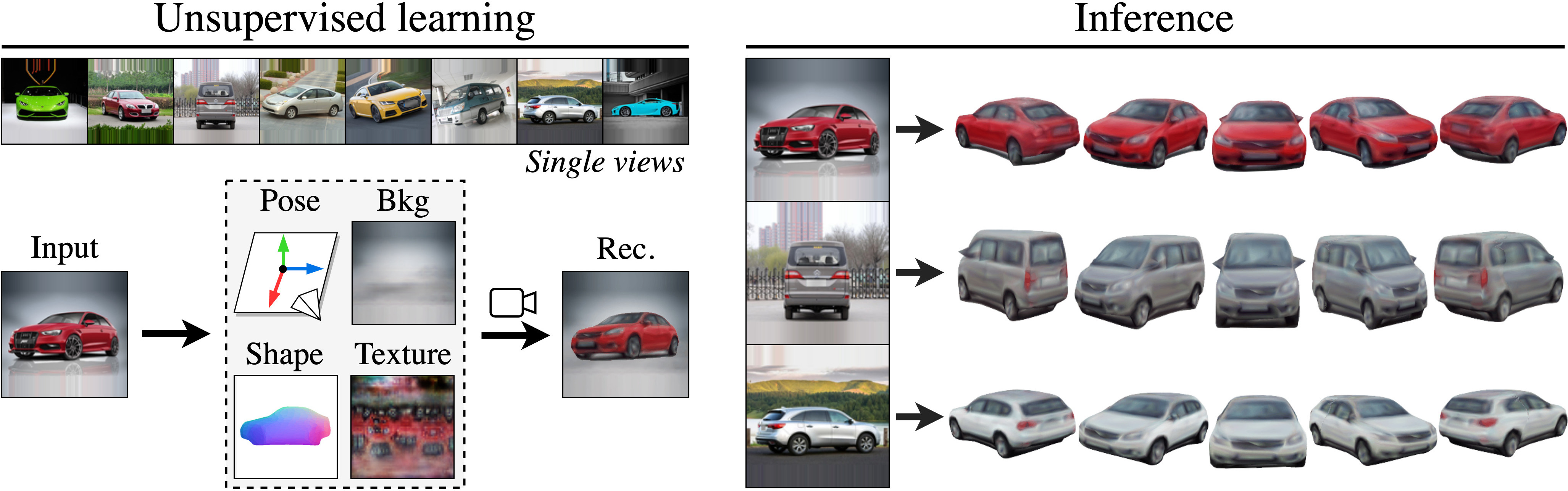
Figure 1: Single-View Reconstruction by Cross-Instance Consistency. (left) Given a collection of single-view images from an object category, we learn without additional supervision an autoencoder that explicitly generates shape, texture, pose and background. (right) At inference time, our approach reconstructs high-quality textured meshes from raw single-view images.

1 Introduction

One of the most magical human perceptual abilities is being able to see the 3D world behind a 2D image – a mathematically impossible task! Indeed, the ancient Greeks were so incredulous at the possibility that humans could be “hallucinating” the third dimension, that they proposed the utterly implausible Emission Theory of Vision [10] (eye emitting light to “sense” the world) to explain it to themselves. In the history of computer vision, single-view reconstruction (SVR) has had an almost cult status as one of the holy grail problems [19, 20, 47]. Recent advancements in deep learning methods have dramatically improved results in this area [6, 37]. However, the best methods still require costly supervision at training time, such as multiple views [35, 44]. Despite efforts to remove such requirements, the works with the least supervision still rely on two signals limiting their applicability: (i) silhouettes and (ii) strong assumptions such as symmetries [25, 21], known template shapes [12, 51], or the absence of background [57]. Although crucial to achieve reasonable results, priors like silhouettes and symmetry can also harm the reconstruction quality: silhouette annotations are often coarse [5] and small symmetry prediction errors can yield unrealistic reconstructions [57, 12].

Method	Supervision	Data	Output
Pix2Mesh [54], AtlasNet [14], OccNet [37]	3D	ShapeNet	3D
PTN [60], NMR [30]	MV, CK, S	ShapeNet	3D
DRC [52], SoftRas [35], DVR [44]	MV, CK, S	ShapeNet	3D, T
GANverse3D [67]	MV, CK, S	Bird, Car, Horse	3D, T
DPC [23], MVC [50]	MV, S	ShapeNet	3D, P
Vicente et al. [53], CSDM [26], DRC [52]	CK, S	Pascal3D	3D
CMR [25]	CK, S, A($\dagger$)	Bird, Car, Plane	3D, T
SDF-SRN[34], TARS [8]	CK, S	ShapeNet, Bird, Car, Plane	3D, T
TexturedMeshGen[17]	CK, A($\dagger$)	ShapeNet, Bird, Car	3D, T
UCMR[12], IMR [51]	S, A($\diamondsuit$, $\dagger$)	Animal, Car, Moto	3D, T, P
UMR [33]	S, A($\leftrightarrow$, $\dagger$)	Animal, Car, Moto	3D, T, P
RADAR [56]	S, A($\ddagger$)	Vase	3D, T, P
SMR [21]	S, A($\dagger$)	ShapeNet, Animal, Moto	3D, T, P
Unsup3D [57]	A($\boxtimes$, $\lessdot$, $\dagger$)	Face	D, T, P
Henderson & Ferrari [16]	A($\boxtimes$, $\varnothing$)	ShapeNet	3D, P
Ours	None	ShapeNet, Animal, Car, Moto	3D, T, P

Table 1: Comparison with selected works. For each method, we outline the supervision and priors used (3D, Multi-Views, Camera or Keypoints, Silhouettes, Assumptions like $\diamondsuit$ template shape, $\dagger$ symmetry, $\ddagger$ solid of revolution, $\leftrightarrow$ semantic consistency, $\boxtimes$ no/limited background, $\lessdot$ frontal view, $\varnothing$ no texture), which data it has been applied to and the model output (3D, Texture, Pose, Depth).

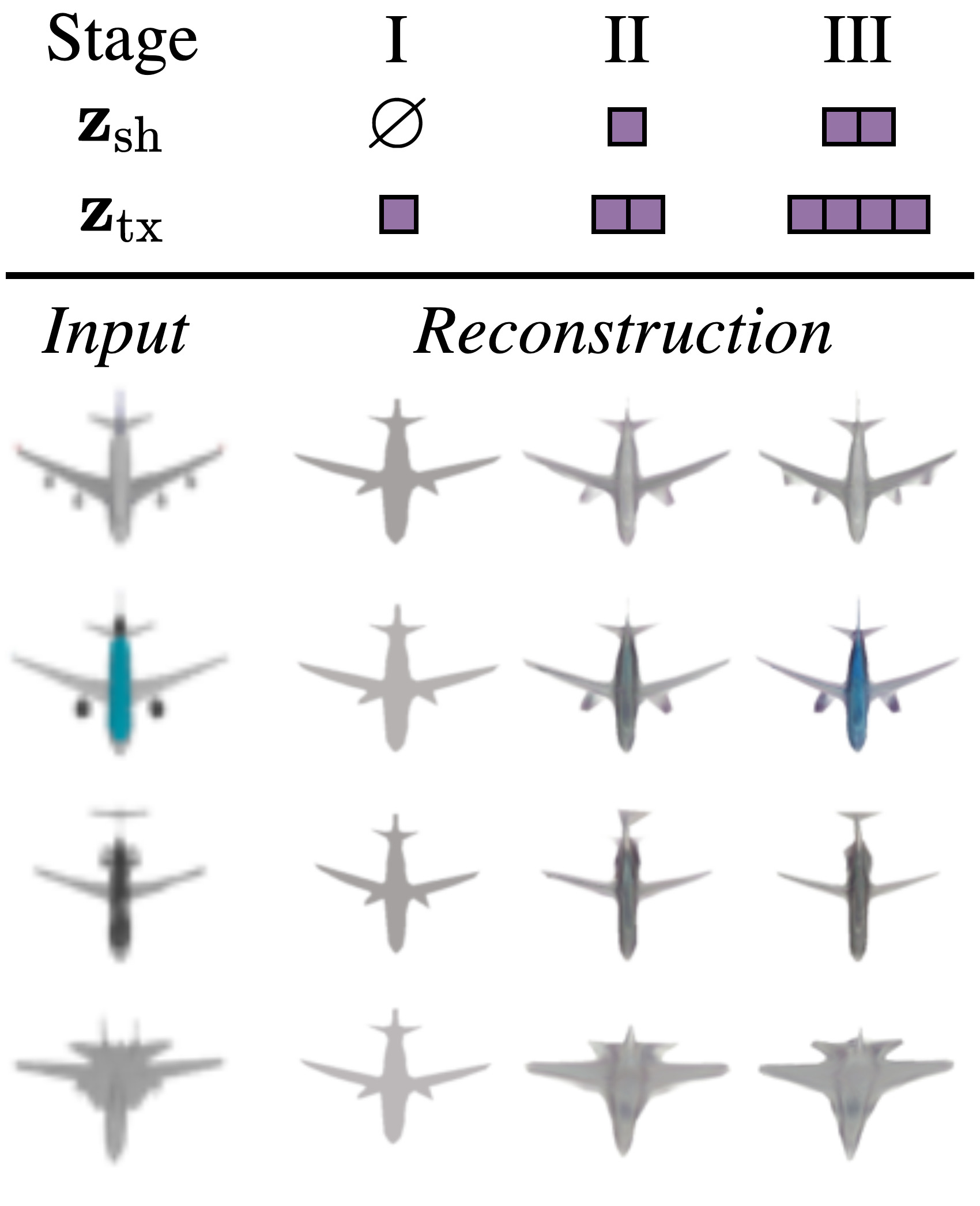
(a) Progressive conditioning

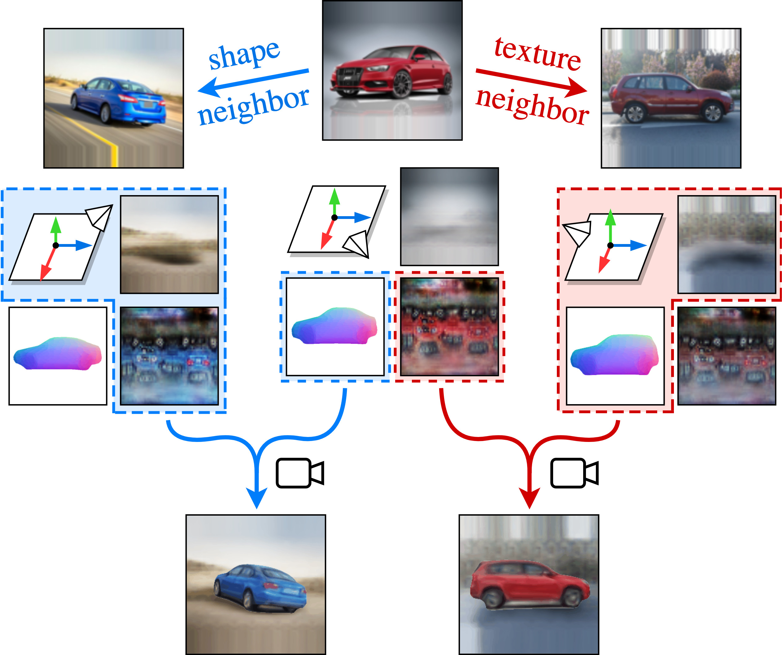
(b) Neighbor reconstruction

Figure 2: Leveraging cross-instance consistency. (a) Progressive conditioning amounts to gradually increasing, in a multi-stage fashion, the size of the conditioning latent spaces, here associated to shape $\mathbf{z}_{\textrm{sh}}$ and texture $\mathbf{z}_{\textrm{tx}}$. (b) We explicitly share the shape and texture models across neighboring instances by swapping their characteristics and applying a loss to associated neighbor reconstructions.

In this paper, we propose the most unsupervised approach to single-view reconstruction to date, which we demonstrate to be competitive for diverse datasets. Table 1 summarizes the differences between our approach and representative prior works. More precisely, we learn in an analysis-by-synthesis fashion a network that predicts for each input image: 1) a 3D shape parametrized as a deformation of an ellipsoid, 2) a texture map, 3) a camera viewpoint, and 4) a background image (Fig. 1). Our main insight to remove the supervision and assumptions required by other methods is to leverage the consistency across different instances. First, we design a training procedure, progressive conditioning, which encourages the model to share elements between images by strongly constraining the variability of shape, texture and background at the beginning of training and progressively allowing for more diversity (Fig. 2(a)). Second, we introduce a neighbor reconstruction loss, which explicitly enforces neighboring instances from different viewpoints to share the same shape or texture model (Fig. 2(b)). Note that these simple yet effective techniques are data-driven and not specific to any dataset. Our only remaining assumption is the knowledge of the semantic class of the depicted object.

We also provide two technical insights that we found critical to learn our model without viewpoint and silhouette annotations: (i) a differentiable rendering formulation inspired by layered image models [24, 39] which we found to perform better than the classical SoftRasterizer [35], and (ii) a new optimization strategy which alternates between learning a set of pose candidates with associated probabilities and learning all other components using the most likely candidate.

We validate our approach on the standard ShapeNet [4] benchmark, real image SVR benchmarks (Pascal3D+ Car [58], CUB [55]) as well as more complex real-world datasets (CompCars [61], LSUN Motorbike and Horse [64]). In all scenarios, we demonstrate results competitive with the best supervised methods.

1.0.1 Summary.

We present UNICORN, a framework leveraging UNsupervised cross-Instance COnsistency for 3D ReconstructioN. Our main contributions are: 1) the most unsupervised SVR system to date, demonstrating state-of-the-art textured 3D reconstructions for both generic shapes and real images, and not requiring supervision or restrictive assumptions beyond a categorical image collection; 2) two data-driven techniques to enforce cross-instance consistency, namely progressive conditioning and neighbor reconstruction. Code and video results are available at imagine.enpc.fr/~monniert/UNICORN.

2 Related work

We first review deep SVR methods and mesh-based differential renderers we build upon. We then discuss works exploring cross-instance consistency and curriculum learning techniques, to which our progressive conditioning is related.

2.0.1 Deep SVR.

There is a clear trend to remove supervision from deep SVR pipelines to directly learn 3D from raw 2D images, which we summarize in Table 1.

A first group of methods uses strong supervision, either paired 3D and images or multiple views of the same object. Direct 3D supervision is successfully used to learn voxels [6], meshes [54], parametrized surfaces [14] and implicit functions [37, 59]. The first methods using silhouettes and multiple views initially require camera poses and are also developed for diverse 3D shape representations: [60, 52] opt for voxels, [30, 35, 5] introduce mesh renderers, and [44] adapts implicit representations. Works like [23, 50] then introduce techniques to remove the assumption of known poses. Except for [67] which leverages GAN-generated images [13, 27], these works are typically limited to synthetic datasets.

A second group of methods aims at removing the need for 3D and multi-view supervision. This is very challenging and they hence typically focus on learning 3D from images of a single category. Early works [53, 26, 52] estimate camera poses with keypoints and minimize the silhouette reprojection error. The ability to predict textures is first incorporated by CMR [25] which, in addition to keypoints and silhouettes, uses symmetry priors. Recent works [34, 8] replace the mesh representation of CMR with implicit functions that do not require symmetry priors, yet the predicted texture quality is strongly deteriorated. [17] improves upon CMR and develops a framework for images with camera annotations that does not rely on silhouettes. Two works managed to further avoid the need for camera estimates but at the cost of additional hypothesis: [16] shows results with textureless synthetic objects, [57] models 2.5D objects like faces with limited background and viewpoint variation. Finally, recent works only require object silhouettes but they also make additional assumptions: [12, 51] use known template shapes, [33] assumes access to an off-the-shelf system predicting part semantics, and [56] targets solids of revolution. Other related works [11, 29, 18, 45, 63, 21] leverage in addition generative adversarial techniques to improve the learning.

In this work, we do not use camera estimates, keypoints, silhouettes, nor strong dataset-specific assumptions, and demonstrate results for both diverse shapes and real images. To the best of our knowledge, we present the first generic SVR system learned from raw image collections.

2.0.2 Mesh-based differentiable rendering.

We represent 3D models as meshes with parametrized surfaces, as introduced in AtlasNet [14] and advocated by [51]. We optimize the mesh geometry, texture and camera parameters associated to an image using differentiable rendering. Loper and Black [36] introduce the first generic differentiable renderer by approximating derivatives with local filters, and [30] proposes an alternative approximation more suitable to learning neural networks. Another set of methods instead approximates the rendering function to allow differentiability, including SoftRasterizer [35, 46] and DIB-R [5]. We refer the reader to [28] for a comprehensive study. We build upon SoftRasterizer [35], but modify the rendering function to learn without silhouette information.

2.0.3 Cross-instance consistency.

Although all methods learned on categorical image collections implicitly leverage the consistency across instances, few recent works explicitly explore such a signal. Inspired by [32], the SVR system of [21] is learned by enforcing consistency between the interpolated 3D attributes of two instances and attributes predicted for the associated reconstruction. [62] discovers 3D parts using the inconsistency of parts across instances. Closer to our approach, [40] introduces a loss enforcing cross-silhouette consistency. Yet it differs from our work in two ways: (i) the loss operates on silhouettes, whereas our loss is adapted to image reconstruction by modeling background and separating two terms related to shape and texture, and (ii) the loss is used as a refinement on top of two cycle consistency losses for poses and 3D reconstructions, whereas we demonstrate results without additional self-supervised losses.

2.0.4 Curriculum learning.

The idea of learning networks by ‘‘starting small’’ dates back to Elman [9] where two curriculum learning schemes are studied: (i) increasing the difficulty of samples, and (ii) increasing the model complexity. We respectively coin them curriculum sampling and curriculum modeling for differentiation. Known to drastically improve the convergence speed [2], curriculum sampling is widely adopted across various applications [48, 1, 22]. On the contrary, curriculum modeling is typically less studied although crucial to various methods. For example, [54] performs SVR in a coarse-to-fine manner by increasing the number of mesh vertices, and [38] clusters images by aligning them with transformations that increase in complexity. We propose a new form of curriculum modeling dubbed progressive conditioning which enables us to avoid bad minima.

3 Approach

Our goal is to learn a neural network that reconstructs a textured 3D object from a single input image. We assume we have access to a raw collection of images depicting objects from the same category, without any further annotation. We propose to learn in an analysis-by-synthesis fashion by autoencoding images in a structured way (Fig. 3). We first introduce our structured autoencoder (Sec. 3.1). We then present how we learn models consistent across instances (Sec. 3.2). Finally, we discuss one more technical contribution necessary to our system: an alternate optimization strategy for joint 3D and pose estimation (Sec. 3.3).

3.0.1 Notations.

We use bold lowercase for vectors (e.g., $\mathbf{a}$), bold uppercase for images (e.g., $\mathbf{A}$), double-struck uppercase for meshes (e.g., ${\mathbb{A}}$), calligraphic uppercase for the main modules of our system (e.g., $\mathcal{A}$), lowercase indexed with generic parameters $\theta$ for networks (e.g., $a_{\theta}$), and write $a_{1:N}$ the ordered set $\{a_{1},\ldots,a_{n}\}$.

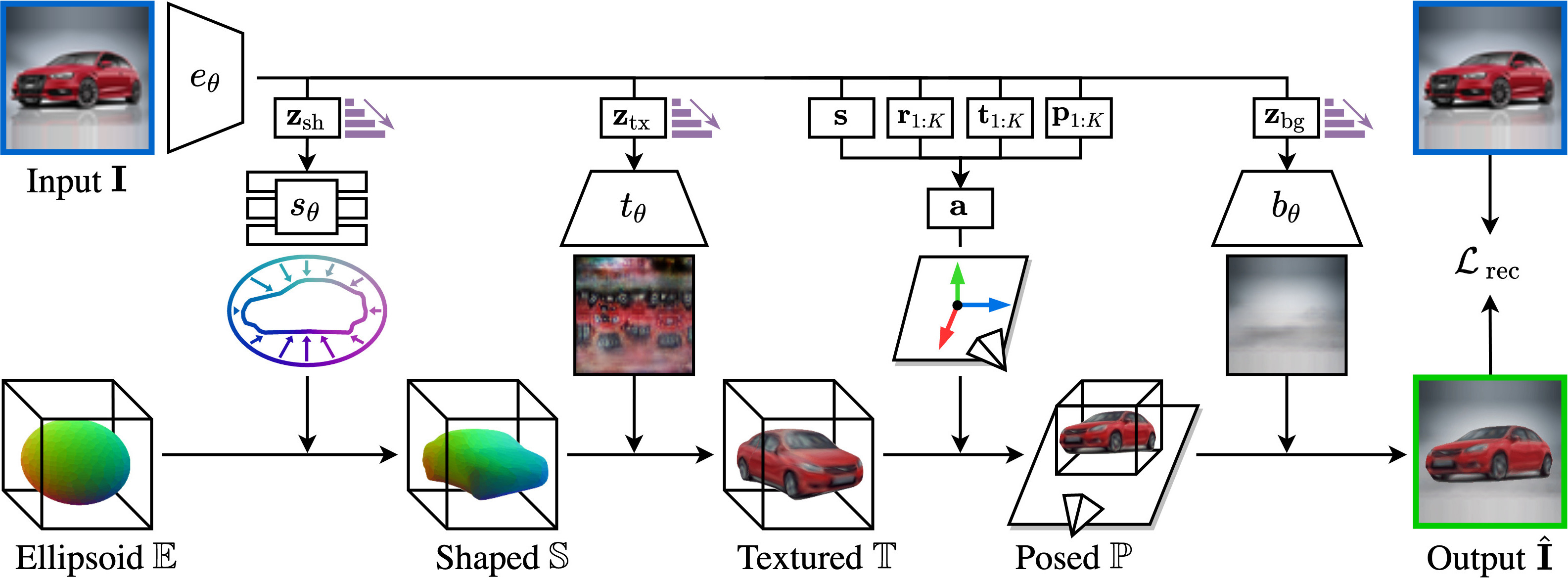
Figure 3: Structured autoencoding. Given an input, we predict parameters that are decoded into 4 factors (shape, texture, pose, background) and composed to generate the output. Progressive conditioning is represented with *X.

3.1 Structured autoencoding

3.1.1 Overview.

Our approach can be seen as a structured autoencoder: it takes an image as input, computes parameters with an encoder, and decodes them into explicit and interpretable factors that are composed to generate an image. We model images as the rendering of textured meshes on top of background images. For a given image $\mathbf{I}$, our model thus predicts a shape, a texture, a pose and a background which are composed to get the reconstruction $\hat{\mathbf{I}}$, as shown in Figure 3. More specifically, the image $\mathbf{I}$ is fed to convolutional encoder networks $e_{\theta}$ which output parameters $e_{\theta}(\mathbf{I})=\{\mathbf{z}_{\textrm{sh}},\mathbf{z}_{\textrm{tx}},\mathbf{a},\mathbf{z}_{\textrm{bg}}\}$ used for the decoding part. $\mathbf{a}$ is a 9D vector including the object pose, while the dimension of the latent codes $\mathbf{z}_{\textrm{sh}},\mathbf{z}_{\textrm{tx}}$ and $\mathbf{z}_{\textrm{bg}}$ will vary during training (see Sec. 3.2). In the following, we describe the decoding modules using these parameters to build the final image by generating a shape, adding texture, positioning it and rendering it over a background.

3.1.2 Shape deformation.

We follow [51] and use the parametrization of AtlasNet [14] where different shapes are represented as deformation fields applied to the unit sphere. We apply the deformation to an icosphere slightly stretched into an ellipsoid mesh ${\mathbb{E}}$ using a fixed anisotropic scaling. More specifically, given a 3D vertex $\mathbf{x}$ of the ellipsoid, our shape deformation module ${\mathcal{S}}_{\mathbf{z}_{\textrm{sh}}}$ is defined by ${\mathcal{S}}_{\mathbf{z}_{\textrm{sh}}}(\mathbf{x})=\mathbf{x}+s_{\theta}(\mathbf{x},\mathbf{z}_{\textrm{sh}}),$ where $s_{\theta}$ is a Multi-Layer Perceptron taking as input the concatenation of a 3D point $\mathbf{x}$ and a shape code $\mathbf{z}_{\textrm{sh}}$. Applying this displacement to all the ellipsoid vertices enables us to generate a shaped mesh ${\mathbb{S}}={\mathcal{S}}_{\mathbf{z}_{\textrm{sh}}}({\mathbb{E}})$. We found that using an ellipsoid instead of a raw icosphere was very effective in encouraging the learning of objects aligned w.r.t. the canonical axes. Learning surface deformations is often preferred to vertex-wise displacements as it enables mapping surfaces, and thus meshes, at any resolution. For us, the mesh resolution is kept fixed and such a representation is a way to regularize the deformations.

3.1.3 Texturing.

Following the idea of CMR [25], we model textures as an image UV-mapped onto the mesh through the reference ellipsoid. More specifically, given a texture code $\mathbf{z}_{\textrm{tx}}$, a convolutional network $t_{\theta}$ is used to produce an image $t_{\theta}(\mathbf{z}_{\textrm{tx}})$, which is UV-mapped onto the sphere using spherical coordinates to associate a 2D point to every vertex of the ellipsoid, and thus to each vertex of the shaped mesh. We write ${\mathcal{T}}_{\mathbf{z}_{\textrm{tx}}}$ this module generating a textured mesh ${\mathbb{T}}={\mathcal{T}}_{\mathbf{z}_{\textrm{tx}}}({\mathbb{S}})$.

3.1.4 Affine transformation.

To render the textured mesh ${\mathbb{T}}$, we define its position w.r.t. the camera. In addition, we found it beneficial to explicitly model an anisotropic scaling of the objects. Because predicting poses is difficult, we predict $K$ poses candidates, defined by rotations $\mathbf{r}_{1:K}$ and translations $\mathbf{t}_{1:K}$, and associated probabilities $\mathbf{p}_{1:K}$. This involves learning challenges we tackle with a specific optimization procedure described in Sec. 3.3. At inference, we select the pose with highest probability. We combine the scaling and the most likely 6D pose in a single affine transformation module ${\mathcal{A}}_{\mathbf{a}}$. More precisely, ${\mathcal{A}}_{\mathbf{a}}$ is parametrized by $\mathbf{a}=\{\mathbf{s},\mathbf{r},\mathbf{t}\}$, where $\mathbf{s},\mathbf{r},\mathbf{t}\in{\rm I\!R}^{3}$ respectively correspond to the three scales of an anisotropic scaling, the three Euler angles of a rotation and the three coordinates of a translation. A 3D point $\mathbf{x}$ on the mesh is then transformed by ${\mathcal{A}}_{\mathbf{a}}(\mathbf{x})=\text{rot}(\mathbf{r})\text{diag}(\mathbf{s})\mathbf{x}+\mathbf{t}$ where $\text{rot}(\mathbf{r})$ is the rotation matrix associated to $\mathbf{r}$ and $\text{diag}(\mathbf{s})$ is the diagonal matrix associated to $\mathbf{s}$. Our module is applied to all points of the textured mesh ${\mathbb{T}}$ resulting in a posed mesh ${\mathbb{P}}={\mathcal{A}}_{\mathbf{a}}({\mathbb{T}})$.

3.1.5 Rendering with background.

The final step of our process is to render the mesh over a background image. The background image is generated from a background code $\mathbf{z}_{\textrm{bg}}$ by a convolutional network $b_{\theta}$. A differentiable module ${\mathcal{B}}_{\mathbf{z}_{\textrm{bg}}}$ renders the posed mesh ${\mathbb{P}}$ over this background image $b_{\theta}(\mathbf{z}_{\textrm{bg}})$ resulting in a reconstructed image $\hat{\mathbf{I}}={\mathcal{B}}_{\mathbf{z}_{\textrm{bg}}}({\mathbb{P}})$. We perform rendering through soft rasterization of the mesh. Because we observed divergence results when learning geometry from raw photometric comparison with the standard SoftRasterizer [35, 46], we propose two key changes: a layered aggregation of the projected faces and an alternative occupancy function. We provide details in our supplementary material.

3.2 Unsupervised learning with cross-instance consistency

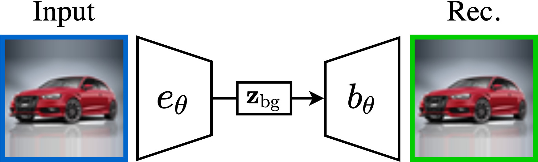
(a) Degenerate background

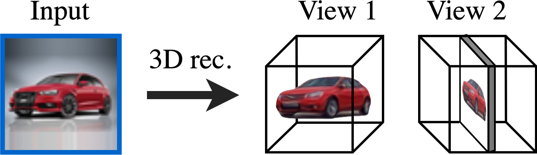
(b) Degenerate 3D object

Figure 4: Degenerate solutions. An SVR system learned by raw image autoencoding is prone to degenerate solutions through (a) the background or (b) the 3D object model. We alleviate the issue with cross-instance consistency.

We propose to learn our structured autoencoder without any supervision, by synthesizing 2D images and minimizing a reconstruction loss. Due to the unconstrained nature of the problem, such an approach typically yields degenerate solutions (Fig. 4(a) and Fig. 4(b)). While previous works leverage silhouettes and dataset-specific priors to mitigate this issue, we instead propose two unsupervised data-driven techniques, namely progressive conditioning (a training strategy) and neighbor reconstruction (a training loss). We thus optimize the shape, texture and background by minimizing for each image $\mathbf{I}$ reconstructed as $\hat{\mathbf{I}}$:

$${\mathcal{L}}_{\textrm{3D}}={\mathcal{L}}_{\textrm{rec}}(\mathbf{I},\hat{\mathbf{I}})+\lambda_{\textrm{nbr}}{\mathcal{L}}_{\textrm{nbr}}+\lambda_{\textrm{reg}}{\mathcal{L}}_{\textrm{reg}},$$ (1)

where $\lambda_{\textrm{nbr}}$ and $\lambda_{\textrm{reg}}$ are scalar hyperparameters, and ${\mathcal{L}}_{\textrm{rec}}$, ${\mathcal{L}}_{\textrm{nbr}}$ and ${\mathcal{L}}_{\textrm{reg}}$ are respectively the reconstruction, neighbor reconstruction, and regularization losses, described below. In all experiments, we use $\lambda_{\textrm{nbr}}=1$ and $\lambda_{\textrm{reg}}=0.01$. Note that we optimize pose prediction using a slightly different loss in an alternate optimization scheme described in Section 3.3.

3.2.1 Reconstruction and regularization losses.

Our reconstruction loss has two terms, a pixel-wise squared $L_{2}$ loss ${\mathcal{L}}_{\textrm{pix}}$ and a perceptual loss [66] ${\mathcal{L}}_{\textrm{perc}}$ defined as an $L_{2}$ loss on the relu3_3 layer of a pre-trained VGG16 [49], similar to [57]. While pixel-wise losses are common for autoencoders, we found it crucial to add a perceptual loss to learn textures that are discriminative for the pose estimation. Our full reconstruction loss can be written ${\mathcal{L}}_{\textrm{rec}}(\mathbf{I},\hat{\mathbf{I}})={\mathcal{L}}_{\textrm{pix}}(\mathbf{I},\hat{\mathbf{I}})+\lambda_{\textrm{perc}}{\mathcal{L}}_{\textrm{perc}}(\mathbf{I},\hat{\mathbf{I}})$ and we use $\lambda_{\textrm{perc}}=10$ in all experiments. While our deformation-based surface parametrization naturally regularizes the shape, we sometimes observe bad minima where the surface has folds. Following prior works [35, 5, 12, 65], we thus add a small regularization term ${\mathcal{L}}_{\textrm{reg}}={\mathcal{L}}_{\textrm{norm}}+{\mathcal{L}}_{\textrm{lap}}$ consisting of a normal consistency loss [7] ${\mathcal{L}}_{\textrm{norm}}$ and a Laplacian smoothing loss [41] ${\mathcal{L}}_{\textrm{lap}}$.

3.2.2 Progressive conditioning.

The goal of progressive conditioning is to encourage the model to share elements (e.g., shape, texture, background) across instances to prevent degenerate solutions. Inspired by the curriculum learning philosophy [9, 54, 38], we propose to do so by gradually increasing the latent space representing the shape, texture and background. Intuitively, restricting the latent space implicitly encourages maximizing the information shared across instances. For example, a latent space of dimension 0 (i.e., no conditioning) amounts to learning a global representation that is the same for all instances, while a latent space of dimension 1 restricts all the generated shapes, textures or backgrounds to lie on a 1-dimensional manifold. Progressively increasing the size of the latent code during training can be interpreted as gradually specializing from category-level to instance-level knowledge.  Figure 2(a) illustrates the procedure with example results where we can observe the progressive specialization to particular instances: reactors gradually appear/disappear, textures get more accurate. Because common neural network implementations have fixed-size inputs, we implement progressive conditioning by masking, stage-by-stage, a decreasing number of values of the latent code. All our experiments share the same 4-stage training strategy where the latent code dimension is increased at the beginning of each stage and the network is then trained until convergence. We use dimensions 0/2/8/64 for the shape code, 2/8/64/512 for the texture code and 4/8/64/256 for the background code. We provide real-image results for each stage in our supplementary material.

3.2.3 Neighbor reconstruction.

The idea behind neighbor reconstruction is to explicitly enforce consistency between different instances. Our key assumption is that neighboring instances with similar shape or texture exist in the dataset. If such neighbors are correctly identified, switching their shape or texture in our generation model should give similar reconstruction results. For a given input image, we hence propose to use its shape or texture attribute in the image formation process of neighboring instances and apply our reconstruction loss on associated renderings. Intuitively, this process can be seen as mimicking a multi-view supervision without actually having access to multi-view images by finding neighboring instances in well-designed latent spaces. Figure 2(b) illustrates the procedure with an example.

More specifically, let $\{\mathbf{z}_{\textrm{sh}},\mathbf{z}_{\textrm{tx}},\mathbf{a},\mathbf{z}_{\textrm{bg}}\}$ be the parameters predicted by our encoder for a given input training image $\mathbf{I}$, let $\Omega$ be a memory bank storing the images and parameters of the last $M$ instances processed by the network. We write $\Omega^{\scaleto{(m)}{6pt}}=\{\mathbf{I}^{\scaleto{(m)}{6pt}},\mathbf{z}_{\textrm{sh}}^{\scaleto{(m)}{6pt}},\mathbf{z}_{\textrm{tx}}^{\scaleto{(m)}{6pt}},\mathbf{a}^{\scaleto{(m)}{6pt}},\mathbf{z}_{\textrm{bg}}^{\scaleto{(m)}{6pt}}\}$ each of these $M$ instances and associated parameters. We first select the closest instance from the memory bank $\Omega$ in the texture (respectively shape) code space using the $L_{2}$ distance, $m_{t}=\operatorname*{argmin}_{m}\|\mathbf{z}_{\textrm{tx}}-\mathbf{z}_{\textrm{tx}}^{\scaleto{(m)}{6pt}}\|_{2}$ (respectively $m_{s}=\operatorname*{argmin}_{m}\|\mathbf{z}_{\textrm{sh}}-\mathbf{z}_{\textrm{sh}}^{\scaleto{(m)}{6pt}}\|_{2}$). We then swap the codes and generate the reconstruction $\hat{\mathbf{I}}_{\textrm{tx}}^{\scaleto{(m_{\textrm{t}})}{6pt}}$ (respectively $\hat{\mathbf{I}}_{\textrm{sh}}^{\scaleto{(m_{\textrm{s}})}{6pt}}$) using the parameters $\{\mathbf{z}_{\textrm{sh}}^{\scaleto{(m_{\textrm{t}})}{6pt}},\mathbf{z}_{\textrm{tx}},\mathbf{a}^{\scaleto{(m_{\textrm{t}})}{6pt}},\mathbf{z}_{\textrm{bg}}^{\scaleto{(m_{\textrm{t}})}{6pt}}\}$ (respectively $\{\mathbf{z}_{\textrm{sh}},\mathbf{z}_{\textrm{tx}}^{\scaleto{(m_{\textrm{s}})}{6pt}},\mathbf{a}^{\scaleto{(m_{\textrm{s}})}{6pt}},\mathbf{z}_{\textrm{bg}}^{\scaleto{(m_{\textrm{s}})}{6pt}}\}$). Finally, we compute the reconstruction loss between the images $\mathbf{I}^{\scaleto{(m_{\textrm{t}})}{6pt}}$ and $\hat{\mathbf{I}}_{\textrm{tx}}^{\scaleto{(m_{\textrm{t}})}{6pt}}$ (respectively $\mathbf{I}^{\scaleto{(m_{\textrm{s}})}{6pt}}$ and $\hat{\mathbf{I}}_{\textrm{sh}}^{\scaleto{(m_{\textrm{s}})}{6pt}}$). Our full loss can thus be written:

$${\mathcal{L}}_{\textrm{nbr}}={\mathcal{L}}_{\textrm{rec}}(\mathbf{I}^{\scaleto{(m_{\textrm{t}})}{6pt}},\hat{\mathbf{I}}_{\textrm{tx}}^{\scaleto{(m_{\textrm{t}})}{6pt}})+{\mathcal{L}}_{\textrm{rec}}(\mathbf{I}^{\scaleto{(m_{\textrm{s}})}{6pt}},\hat{\mathbf{I}}_{\textrm{sh}}^{\scaleto{(m_{\textrm{s}})}{6pt}}).$$ (2)

Note that we recompute the parameters of the selected instances with the current network state, to avoid uncontrolled effects of changes in the network state. Also note that, for computational reasons, we do not use this loss in the first stage where codes are almost the same for all instances.

To prevent latent codes from specializing by viewpoint, we split the viewpoints into $V$ bins w.r.t. the rotation angle, uniformly sample a target bin for each input and look for the nearest instances only in the subset of instances within the target viewpoint range (see the supplementary for details). In all experiments, we use $V=5$ and a memory bank of size $M=1024$.

3.3 Alternate 3D and pose learning

Because predicting 6D poses is hard due to self-occlusions and local minima, we follow prior works [23, 16, 12, 51] and predict multiple pose candidates and their likelihood. However, we identify failure modes in their optimization framework (detailed in our supplementary material) and instead propose a new optimization that alternates between 3D and pose learning. More specifically, given an input image $\mathbf{I}$, we predict $K$ pose candidates $\{(\mathbf{r}_{1},\mathbf{t}_{1}),\ldots,(\mathbf{r}_{K},\mathbf{t}_{K})\}$, and their associated probabilities $\mathbf{p}_{1:K}$. We render the model from the different poses, yielding $K$ reconstructions $\hat{\mathbf{I}}_{1:K}$. We then alternate the learning between two steps: (i) the 3D-step where shape, texture and background branches of the network are updated by minimizing ${\mathcal{L}}_{\textrm{3D}}$ using the pose associated to the highest probability, and (ii) the P-step where the branches of the network predicting candidate poses and their associated probabilities are updated by minimizing:

$$\textstyle{\mathcal{L}}_{\textrm{P}}=\sum_{k}\mathbf{p}_{k}{\mathcal{L}}_{\textrm{rec}}(\mathbf{I},\hat{\mathbf{I}}_{k})+\lambda_{\textrm{uni}}{\mathcal{L}}_{\textrm{uni}},$$ (3)

where ${\mathcal{L}}_{\textrm{rec}}$ is the reconstruction loss described in Sec. 3.2, ${\mathcal{L}}_{\textrm{uni}}$ is a regularization loss on the predicted poses and $\lambda_{\textrm{uni}}$ is a scalar hyperparameter. More precisely, we use ${\mathcal{L}}_{\textrm{uni}}=\sum_{k}|\bar{\mathbf{p}}_{k}-\nicefrac{{1}}{{K}}|$ where $\bar{\mathbf{p}}_{k}$ is the averaged probabilities for candidate $k$ in a particular training batch. Similar to [16], we found it crucial to introduce this regularization term to encourage the use of all pose candidates. In particular, this prevents a collapse mode where only few pose candidates are used. Note that we do not use the neighbor reconstruction loss nor the mesh regularization loss which are not relevant for viewpoints. In all experiments, we use $\lambda_{\textrm{uni}}=0.02$.

Inspired by the camera multiplex of [12], we parametrize rotations with the classical Euler angles (azimuth, elevation and roll) and rotation candidates correspond to offset angles w.r.t. reference viewpoints. Since in practice elevation has limited variations, our reference viewpoints are uniformly sampled along the azimuth dimension. Note that compared to [12], we do not directly optimize a set of pose candidates per training image, but instead learn a set of $K$ predictors for the entire dataset. We use $K=6$ in all experiments.

4 Experiments

We validate our approach in two standard setups. It is first quantitatively evaluated on ShapeNet where state-of-the-art methods use multiple views as supervision. Then, we compare it on standard real-image benchmarks and demonstrate its applicability to more complex datasets. Finally, we present an ablation study.

4.1 Evaluation on the ShapeNet benchmark

We compare our approach to state-of-the-art methods using multi-views, viewpoints and silhouettes as supervision. Our method is instead learned without supervision. For all compared methods, one model is trained per class. We adhere to community standards [30, 35, 44] and use the renderings and splits from [30] of the ShapeNet dataset [4]. It corresponds to a subset of 13 classes of 3D objects, each object being rendered into a $64\times 64$ image from 24 viewpoints uniformly spaced along the azimuth dimension. We evaluate all methods using the standard Chamfer-$L_{1}$ distance [37, 44], where predicted shapes are pre-aligned using our gradient-based version of the Iterative Closest Point (ICP) [3] with anisotropic scaling. Indeed, compared to competing methods having access to the ground-truth viewpoint during training, we need to predict it for each input image in addition to the 3D shape. This yields to both shape/pose ambiguities (e.g., a small nearby object or a bigger one far from the camera) and small misalignment errors that dramatically degrade the performances. We provide evaluation details as well as results without ICP in our supplementary.

We report quantitative results and compare to the state of the art in Figure 6, where methods using multi-views are visually separated. We evaluate the pre-trained weights for SDF-SRN [34] and train the models from scratch using the official implementation for DVR [44]. We tried evaluating SMR [21] but could not reproduce the results. We do not compare to TARS [8] which is based on SDF-SRN and share the same performances. Our approach achieves results that are on average better than the state-of-the-art methods supervised with silhouette and viewpoint annotations. This is a strong result: while silhouettes are trivial in this benchmark, learning without viewpoint annotations is extremely challenging as it involves solving the pose estimation and shape reconstruction problems simultaneously. For some categories, our performances are even better than DVR supervised with multiple views. This shows that our system learned on raw images generates 3D reconstructions comparable to the ones obtained from methods using geometry cues like silhouettes and multiple views. Note that for the lamp category, our method predicts degenerate 3D shapes; we hypothesize this is due to their rotation invariance which makes the viewpoint estimation ambiguous.

We visualize and compare the quality of our 3D reconstructions in Figure 6. The first three examples correspond to examples advertised in DVR [44], the last two corresponds to examples we selected. Our method generates textured meshes of high-quality across all these categories. The geometry obtained is sharp and accurate, and the predicted texture mostly corresponds to the input.

[0.6] Method Ours SDF-SRN [34] DVR [44] DVR [44] MV ✓ CK ✓ ✓ ✓ S ✓ ✓ ✓ airplane 0.110 0.128 0.114 0.111 bench 0.159 - 0.255 0.176 cabinet 0.137 - 0.254 0.158 car 0.168 0.150 0.203 0.153 chair 0.253 0.262 0.371 0.205 display 0.220 - 0.257 0.163 lamp 0.523 - 0.363 0.281 phone 0.127 - 0.191 0.076 rifle 0.097 - 0.130 0.083 sofa 0.192 - 0.321 0.160 speaker 0.224 - 0.312 0.215 table 0.243 - 0.303 0.230 vessel 0.155 - 0.180 0.151 mean 0.201 - 0.250 0.166

Figure 5: ShapeNet comparison. We report Chamfer-$L_{1}\downarrow$ obtained after ICP, best results are highlighted. Supervisions are: Multi-Views, Camera or Keypoints, Silhouettes.

[0.36]

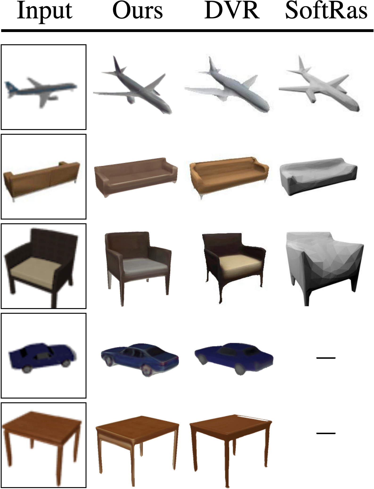
Figure 6: Visual comparisons. We compare to DVR [44] and SoftRas [35] learned with full supervision (MV, CK, S).

4.2 Results on real images

4.2.1 Pascal3D+ Car and CUB benchmarks.

We compare our approach to state-of-the-art SVR methods on real images, where multiple views are not available. All competing methods use silhouette supervision and output meshes that are symmetric. CMR [25] additionally use keypoints, UCMR [12] and IMR [51] starts learning from a given template shape; we do not use any of these and directly learn from raw images. We strictly follow the community standards [25, 12, 51] and use the train/test splits of Pascal3D+ Car [58] (5000/220 images) and CUB-200-2011 [55] (5964/2874 images). Images are square-cropped around the object using bounding box annotations and resized to $64\times 64$.

	Supervision			Pascal3D+ Car			CUB-200-2011
Method	CK	S	A	3D IoU $\uparrow$	Ch-$L_{1}$ $\downarrow$	Mask IoU $\uparrow$	PCK@0.1 $\uparrow$	Mask IoU $\uparrow$
CMR [25]	✓	✓	✓	64	-	-	48.3	70.6
IMR [51]		✓	✓	-	-	-	53.5	-
UMR [33]		✓	✓	62	-	-	58.2	73.4
UCMR [12]		✓	✓	67.3	0.172	73.7	-	63.7
SMR [21]		✓	✓	-	-	-	62.2	80.6
Ours				65.9	0.163	83.9	49.0	71.4

Table 2: Real-image quantitative comparisons. Supervision corresponds to Camera or Keypoints, Silhouettes, Assumptions (see Tab. 1 for details).

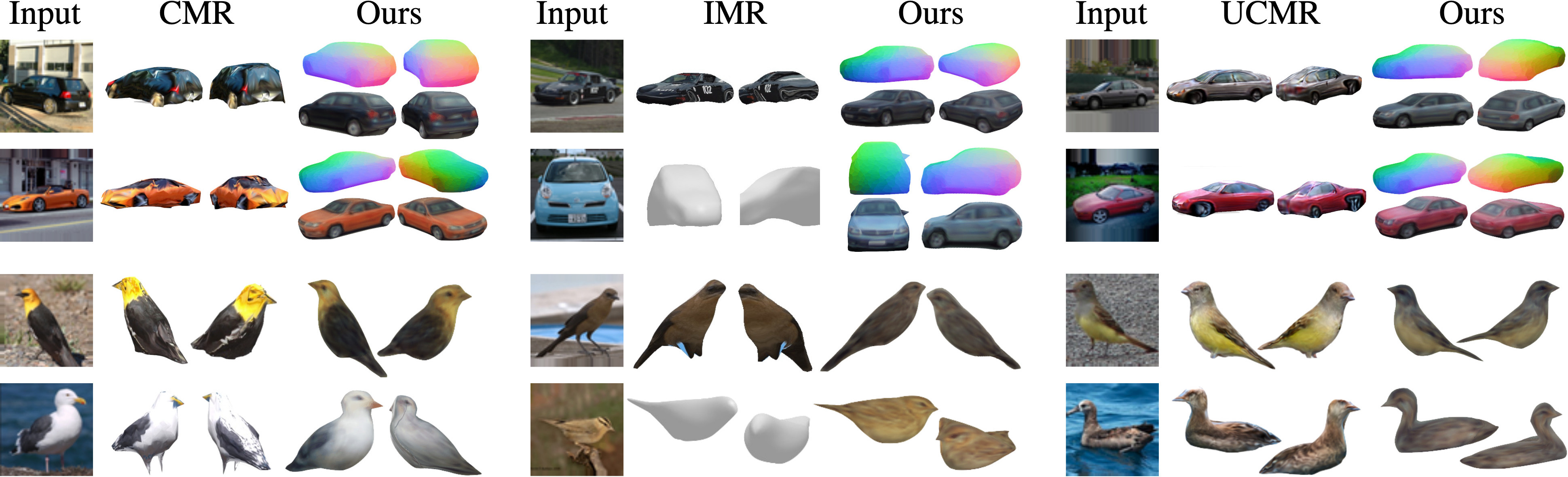
Figure 7: Real-image comparisons. We show reconstructions on Pascal3D+ Cars (top) and CUB (bottom) and compare to CMR [25], IMR [51], UCMR [12].

A quantitative comparison is summarized in Table 2, where we report 3D IoU, Chamfer-$L_{1}$ (with ICP alignment), Mask IoU for Pascal3D+ Car, and Percentage of Correct Keypoints thresholded at $\alpha=0.1$ (PCK@0.1) [32], Mask IoU for CUB. Our approach yields competitive results across all metrics although it does not rely on any supervision used by other works. On Pascal3D+ Car, we achieve significantly better results than UCMR for Chamfer-$L_{1}$ and Mask IoU, which we argue are less biased metrics than the standard 3D IoU [52, 25] computed on unaligned shapes (see supplementary). On CUB, our approach achieves reasonable results that are however slightly worse than the state of the art. We hypothesize this is linked to our pose regularization term encouraging the use of all viewpoints whereas these bird images clearly lack back views.

We qualitatively compare our approach to the state of the art in Figure 7. For each input, we show the mesh rendered from two viewpoints. For our car results, we additionally show meshes with synthetic textures to emphasize correspondences. Qualitatively, our approach yields results on par with prior works both in terms of geometric accuracy and overall realism. Although the textures obtained in [51] look more accurate, they are modeled as pixel flows, which has a clear limitation when synthesizing unseen texture parts. Note that we do not recover details like the bird legs which are missed by prior works due to coarse silhouette annotations. We hypothesize we also miss them because they are hardly consistent across instances, e.g., legs can be bent in multiple ways.

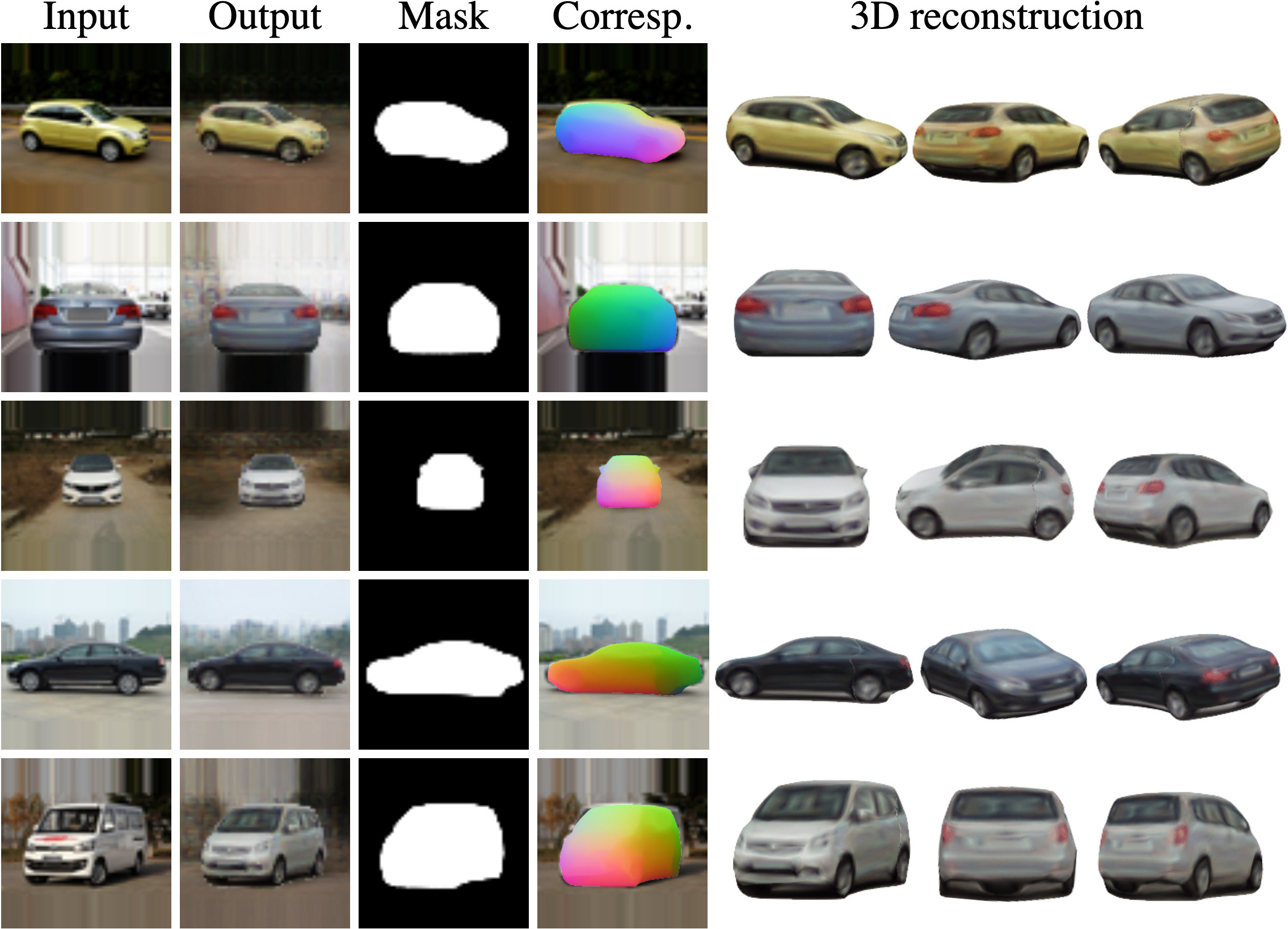
(a) CompCars [61]

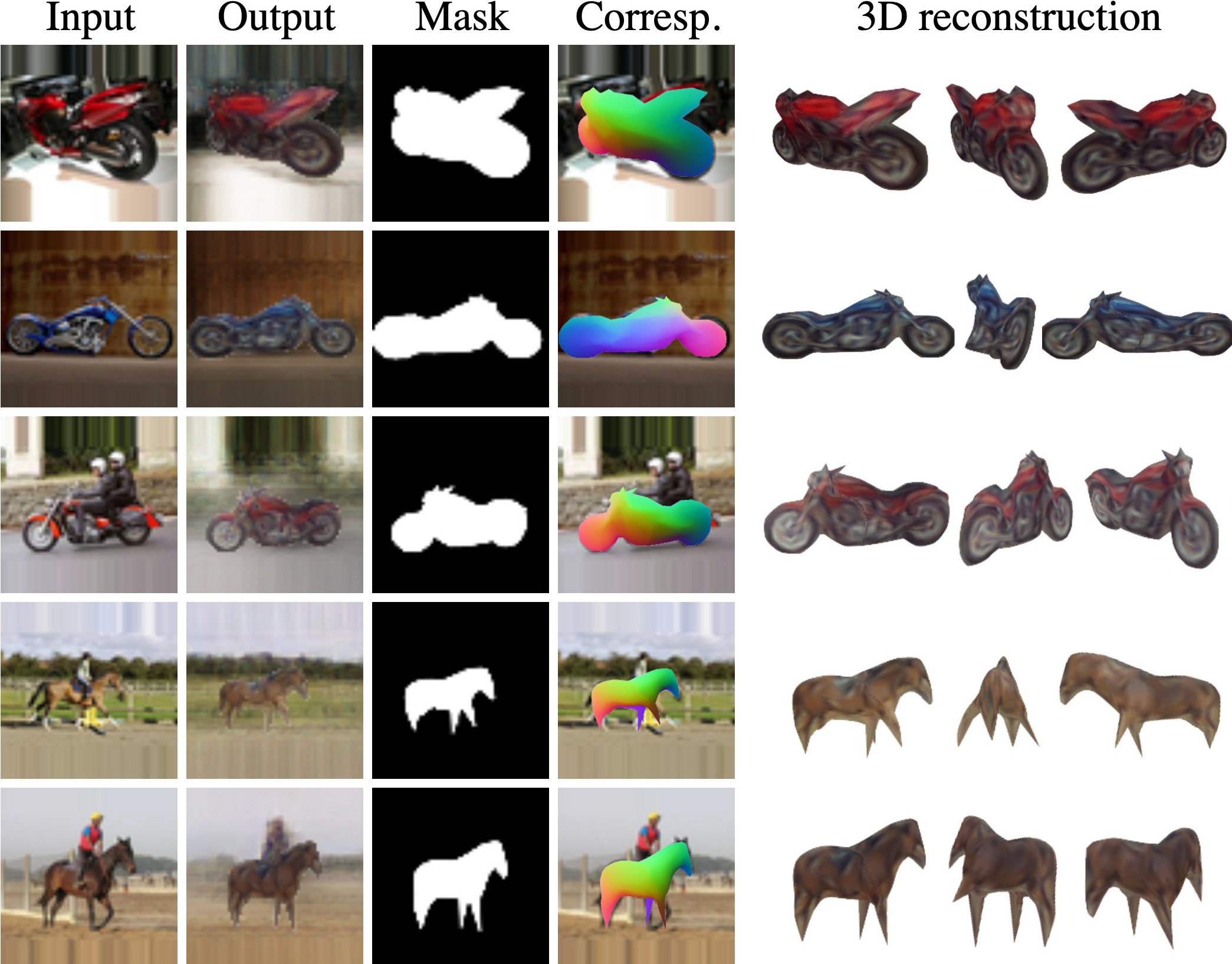
(b) LSUN Motorbike and Horse [64]

Figure 8: Real-world dataset results. From left to right, we show: input and output images, the predicted mask, a correspondence map and the mesh rendered from 3 viewpoints. Note that for LSUN Horse, the geometry quality is low and outlines our approach limitations (see text). Best viewed digitally.

4.2.2 Real-word datasets.

Motivated by 3D-aware image synthesis methods learned in-the-wild [42, 43], we investigate whether our approach can be applied to real-world datasets where silhouettes are not available and images are not methodically cropped around the object. We adhere to standards from the 3D-aware image synthesis community [42, 43] and apply our approach to $64\times 64$ images of CompCars [61]. In addition, we provide results for the more difficult scenario of LSUN images [64] for motorbikes and horses. Because many LSUN images are noise, we filter the datasets as follows: we manually select 16 reference images with different poses, find the nearest neighbors from the first 200k images in a pre-trained ResNet-18 [15] feature space, and keep the top 2k for each reference image. We repeat the procedure with flipped reference images yielding 25k images.

Our results are shown in Figure 8. For each input image, we show from left to right: the output image, the predicted mask, a correspondence map, and the 3D reconstruction rendered from the predicted viewpoint and two other viewpoints. Although our approach is trained to synthesize images, these are all natural by-products. While the quality of our 3D car reconstructions is high, the reconstructions obtained for LSUN images lack some realism and accuracy (especially for horses), thus outlining limitations of our approach. However, our segmentation and correspondence maps emphasize our system ability to accurately localize the object and find correspondences, even when the geometry is coarse.

4.2.3 Limitations.

Even if our approach is a strong step towards generic unsupervised SVR, we can outline three main limitations. First, the lack of different views in the data harms the results (e.g., most CUB birds have concave backs); this can be linked to our uniform pose regularization term which is not adequate in these cases. Second, complex textures are not predicted correctly (e.g., motorbikes in LSUN). Although we argue it could be improved by more advanced autoencoders, the neighbor reconstruction term may prevent unique textures to be generated. Finally, despite its applicability to multiple object categories and diverse datasets, our multi-stage progressive training is cumbersome and an automatic way of progressively specializing to instances is much more desirable.

[0.356] Model Full w/o w/o ${\mathcal{L}}_{\textrm{nbr}}$ PC airplane 0.110 0.124 0.107 bench 0.159 0.188 0.206 car 0.168 0.179 0.173 chair 0.253 0.319 0.527 table 0.243 0.246 0.598 mean 0.187 0.211 0.322   [0.56]

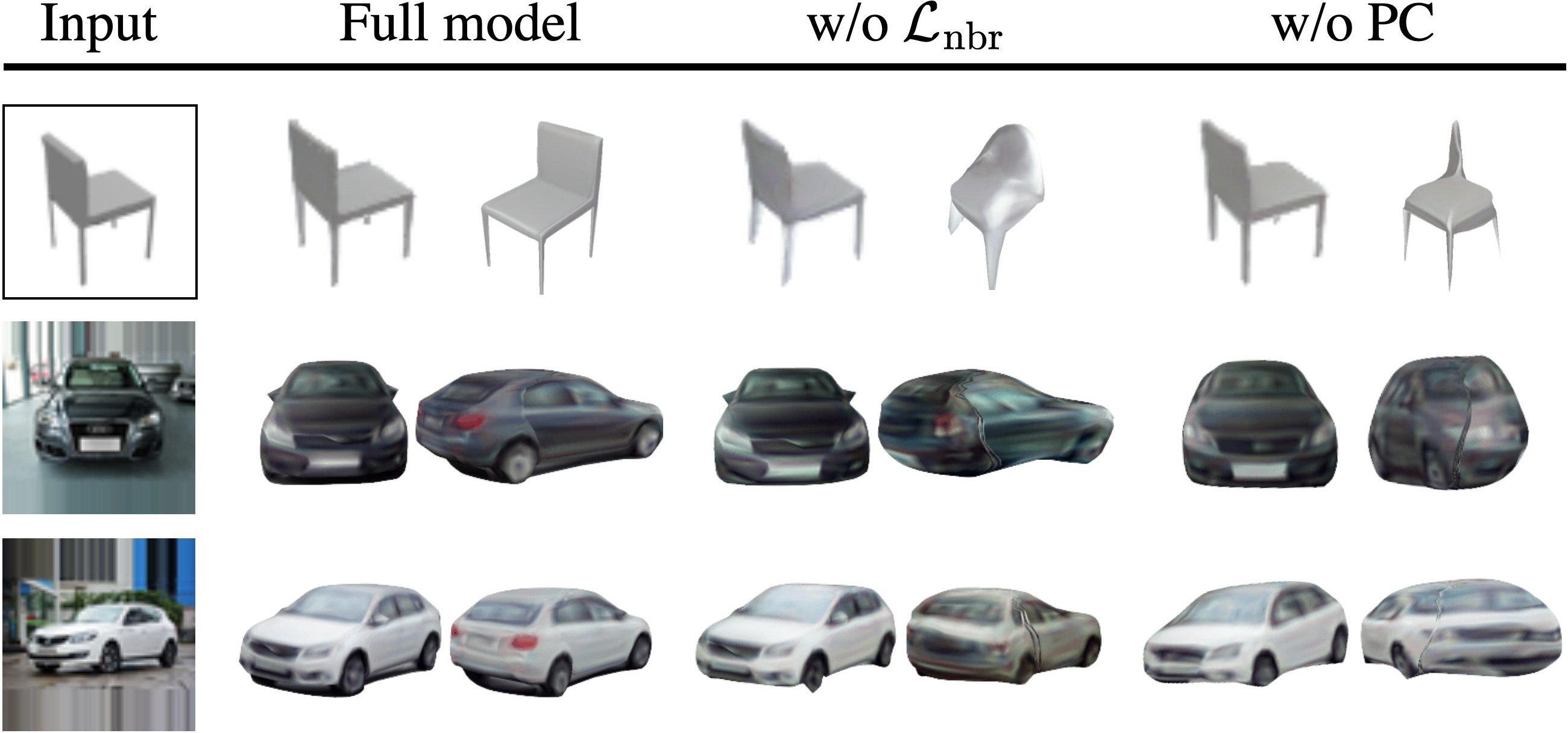
Figure 9: Ablation results on ShapeNet[4].

Figure 10: Ablation visual results. For each input, we show the mesh rendered from two viewpoints.

4.3 Ablation study

We analyze the influence of our neighbor reconstruction loss ${\mathcal{L}}_{\textrm{nbr}}$ and progressive conditioning (PC) by running experiments without each component.

First, we provide quantitative results on ShapeNet in Figure 10. When ${\mathcal{L}}_{\textrm{nbr}}$ is removed, the results are worse for almost all categories, outlining that it is important to the predicted geometry accuracy. When PC is removed, results are comparable to the full model for airplane and car but much worse for chair and table. Indeed, they involve more complex shapes and our system falls into a bad minimum with degenerate solutions, a scenario that is avoided with PC.

Second, we perform a visual comparison on ShapeNet and CompCars examples in Figure 10. For each input, we show the mesh rendered from the predicted viewpoint and a different viewpoint. When ${\mathcal{L}}_{\textrm{nbr}}$ is removed, we observe that the reconstruction seen from the predicted viewpoint is correct but it is either wrong for chairs and degraded for cars when seen from the other viewpoint. Indeed, the neighbor reconstruction explicitly enforces the unseen reconstructed parts to be consistent with other instances. When PC is removed, we observe degenerate reconstructions where the object seen from a different viewpoint is not realistic.

5 Conclusion

We presented UNICORN, an unsupervised SVR method which, in contrast to all prior works, learns from raw images only. We demonstrated it yields high-quality results for diverse shapes as well as challenging real-world image collections. This was enabled by two key contributions aiming at leveraging consistency across different instances: our progressive conditioning training strategy and neighbor reconstruction loss. We believe our work includes both an important step forward for unsupervised SVR and the introduction of a valuable conceptual insight.

5.0.1 Acknowledgements.

We thank François Darmon for inspiring discussions; Robin Champenois, Romain Loiseau, Elliot Vincent for manuscript feedback; Michael Niemeyer, Shubham Goel for evaluation details. This work was supported in part by ANR project EnHerit ANR-17-CE23-0008, project Rapid Tabasco, gifts from Adobe and HPC resources from GENCI-IDRIS (2021-AD011011697R1).

Supplementary Material for
Share With Thy Neighbors: Single-View
Reconstruction by Cross-Instance Consistency

In this supplementary document, we first describe our custom differentiable rendering function (Appendix 0.A). Then, we present additional model insights (Appendix 0.B) as well as quantitative evaluation details (Appendix 0.C). Finally, we provide implementation details (Appendix 0.D), including network architectures, design choices and training details.

Appendix 0.A Custom differentiable rendering

Our output images correspond to the soft rasterization of a textured mesh on top of a background image. We observe divergence results when learning geometry from raw photometric comparison with the standard SoftRasterizer [35] and thus propose two key changes. In the following, given a mesh ${\mathbb{M}}$ and a background $\mathbf{B}$, we describe our rendering function ${\mathcal{R}}$ producing the image $\hat{\mathbf{I}}={\mathcal{R}}({\mathbb{M}},\mathbf{B})$. We first present SoftRasterizer formulation and its limitations, then introduce our modifications. In the following, we write pixel-wise multiplication with $\odot$ and the division of image-sized tensors corresponds to pixel-wise division.

0.A.0.1 SoftRasterizer formulation.

Given a 2D pixel location $i$, the influence of a face $j$ is modeled by an occupancy function:

$${\mathcal{O}}_{\textrm{SR}}(i,j)=\operatorname*{sigmoid}\Big{(}\frac{\nu(i,j)}{\sigma}\Big{)},$$ (4)

where $\sigma$ is a temperature, $\nu(i,j)$ is the signed Euclidean distance between pixel $i$ and projected face $j$. Let us call $L-1$ the maximum number of faces intersecting the ray associated to a pixel and sort, for each pixel, the intersecting faces by increasing depth. Image-sized maps for occupancy $\mathbf{O}_{\ell}$, color $\mathbf{C}_{\ell}$ and depth $0pt_{\ell}$ are built associating to each pixel the $\ell$-th intersecting face attributes. Background is modeled as additional maps such that $\mathbf{O}_{L}=1,\mathbf{C}_{L}=\mathbf{B}$, and $0pt_{L}=d_{\textrm{bg}}$ is a constant, far from the camera. The SoftRasterizer’s aggregation function ${\mathcal{C}}_{\textrm{SR}}$ merges them to render the final image $\hat{\mathbf{I}}$:

$${\mathcal{C}}_{\textrm{SR}}(\mathbf{O}_{1:L},\mathbf{C}_{1:L},0pt_{1:L})=\sum_{\ell=1}^{L}\frac{\mathbf{O}_{\ell}\odot\exp(0pt^{\prime}_{\ell}/\gamma)}{\sum_{k}\mathbf{O}_{k}\odot\exp(0pt^{\prime}_{k}/\gamma)}\;\odot\mathbf{C}_{\ell},$$ (5)

where $\gamma$ is a temperature parameter, $0pt^{\prime}_{\ell}=\frac{d_{\textrm{far}}-0pt_{\ell}}{d_{\textrm{far}}-d_{\textrm{near}}}$ and $d_{\textrm{near}},d_{\textrm{far}}$ correspond to near/far cut-off distances. This formulation hence relies on 5 hyperparameters ($\sigma$, $\gamma$, $d_{\textrm{near}}$, $d_{\textrm{far}}$, $d_{\textrm{bg}}$) and default values are $\sigma=\gamma=10^{-4}$, $d_{\textrm{near}}=1$, $d_{\textrm{far}}=100$ and $\frac{d_{\textrm{far}}-d_{\textrm{bg}}}{d_{\textrm{far}}-d_{\textrm{near}}}=\epsilon=10^{-3}$.

The formulation introduced in Equation 5 has one main limitation: gradients don’t flow well through $\mathbf{O}_{1:L}$ obtained by soft rasterization, and thus vertex positions cannot be optimized by raw photometric comparison. The simple case of a single face on a black background gives:

$$\hat{\mathbf{I}}=\frac{\mathbf{O}_{1}\odot e^{\nicefrac{{0pt^{\prime}_{1}}}{{\gamma}}}}{\mathbf{O}_{1}\odot e^{\nicefrac{{0pt^{\prime}_{1}}}{{\gamma}}}+e^{\nicefrac{{\epsilon}}{{\gamma}}}}\;\odot\mathbf{C}_{1}\approx\frac{\mathbf{O}_{1}\odot e^{\nicefrac{{0pt^{\prime}_{1}}}{{\gamma}}}}{\mathbf{O}_{1}\odot e^{\nicefrac{{0pt^{\prime}_{1}}}{{\gamma}}}}\;\odot\mathbf{C}_{1}=\mathbf{C}_{1},$$ (6)

for almost all $\mathbf{O}_{1},0pt^{\prime}_{1}$. Indeed, considering $x,\eta>0$, we have $xe^{\nicefrac{{(\epsilon+\eta)}}{{\gamma}}}\gg e^{\nicefrac{{\epsilon}}{{\gamma}}}$ iif $x\gg e^{\nicefrac{{-\eta}}{{\gamma}}}$. Even in the best case where $\eta=\epsilon=10^{-3}$ (i.e., the object is close to $d_{\textrm{far}}$), this holds for all $x\gg e^{-10}\approx 4\times 10^{-5}$! We found that tuning $\gamma$ was not sufficient to mitigate the issue, one would have to tune $\gamma,d_{\textrm{near}},d_{\textrm{far}},d_{\textrm{bg}}$ simultaneously to enable the optimization of the vertex positions.

0.A.0.2 Our layered formulation.

Inspired by layered image models [24, 39], we propose to model the rendering of a mesh as the layered composition of its projected face attributes. More specifically, given occupancy $\mathbf{O}_{1:L}$ and color $\mathbf{C}_{1:L}$ maps, we render an image $\hat{\mathbf{I}}$ through the classical recursive alpha compositing:

$${\mathcal{C}}(\mathbf{O}_{1:L},\mathbf{C}_{1:L})=\sum_{\ell=1}^{L}\Big{[}\prod_{k<\ell}^{L}(1-\mathbf{O}_{k})\Big{]}\odot\mathbf{O}_{\ell}\odot\mathbf{C}_{\ell}.$$ (7)

This formulation has a clear interpretation where color maps are overlaid on top of each other with a transparency corresponding to their occupancy map. Note that we choose to drop the explicit depth dependency as all 3D coordinates (including depth) of a vertex already receive gradients by 3D-to-2D projection. Our layered aggregation used together with the SoftRasterizer’s occupancy function ${\mathcal{O}}_{\textrm{SR}}$ results in face inner-borders that are visually unpleasant. We thus instead use the occupancy function introduced in [5] defined by:

$${\mathcal{O}}(i,j)=\exp(\min(0,\frac{\nu(i,j)}{\sigma})).$$ (8)

Compared to ${\mathcal{O}}_{\textrm{SR}}$, this function yields constant occupancy of 1 inside the faces. In addition to its simplicity, our differential renderer has two main advantages compared to SoftRasterizer. First, gradients can directly flow through occupancies $\mathbf{O}_{1:L}$ and the vertex positions can be updated by photometric comparison. Second, our formulation involves only one hyperparameter ($\sigma$) instead of five, making it easier to use.

Appendix 0.B Model insights

0.B.1 Progressive conditioning

Figure 11 shows the results obtained on CompCars [61] at the end of each stage of the training. Given an input image (leftmost column), we show for each training stage the predicted outputs. From left to right, they correspond to a side view of the shape, the texture image and the background image. We can observe that all shape, texture and background models gradually specialize to the instance represented in the input. In particular, this allows us to start with a weak background model to avoid degenerate solutions and to end up with a powerful background model to improve the reconstruction quality. Also note how all the texture images are aligned.

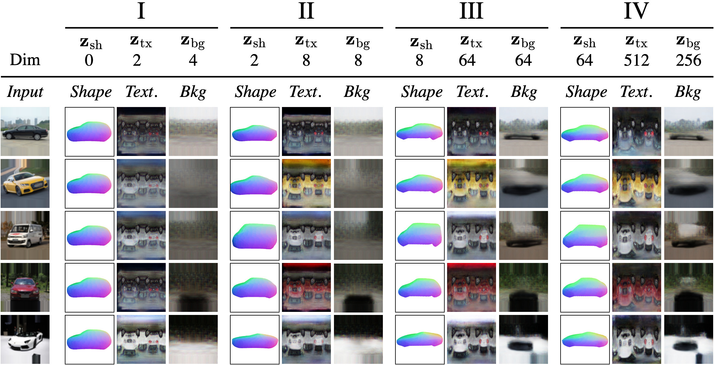
Figure 11: Progressive conditioning on CompCars [61]. Given an input image (leftmost column), we show for each training stage, from left to right, a side view of the predicted shape, the texture image and the background image.

0.B.2 Neighbor reconstruction

When computing the neighbor reconstructions, we explicitly find neighbors that have a viewpoint different from the predicted viewpoint. More specifically, for a given input, we compute the angle between the predicted rotation matrix and all rotation matrices of the memory bank. Following standard conventions, such an angle lies in $[0^{\circ},180^{\circ}]$. Then, we select a target angle range as follows: we split the range of angles $[20^{\circ},180^{\circ}]$ into a partition of $V$ uniform and continuous bins, and we uniformly sample one of the $V$ angle ranges. Finally, we look for neighbors in the subset of instances having an angle within the selected range. In all experiments, we use $V=5$.

We use a total angle range of $[20^{\circ},180^{\circ}]$ instead of $[0^{\circ},180^{\circ}]$ to remove instances having a similar pose. Note that we first tried to find neighbors of different poses without further constraint (which amounts to using $V=1$) but we found that learned latent codes were specialized by viewpoints, e.g., front / back view images corresponding to a shape mode with unrealistic side views, and side view images corresponding to a shape mode with unrealistic front / back views.

0.B.3 Joint 3D and pose learning

We analyze prior works on joint 3D and pose learning, illustrated in Figure 12, and compare them with our proposed optimization scheme, illustrated in Figure 13. Prior optimization schemes can be split in two groups: (i) learning through the minimal error reconstruction [23], and (ii) learning through an expected error [16, 12, 51].

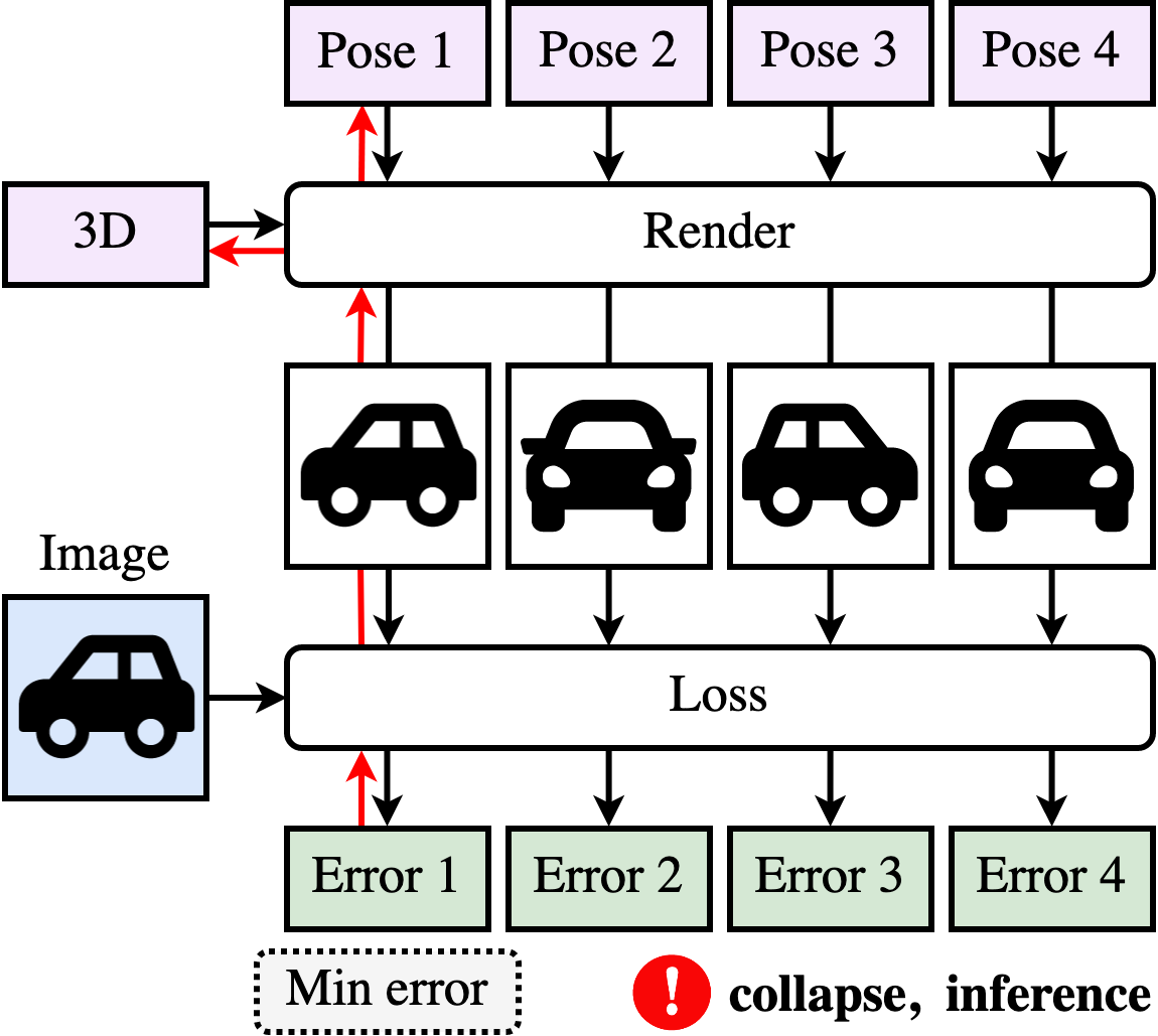
(a) Optimization in [23]

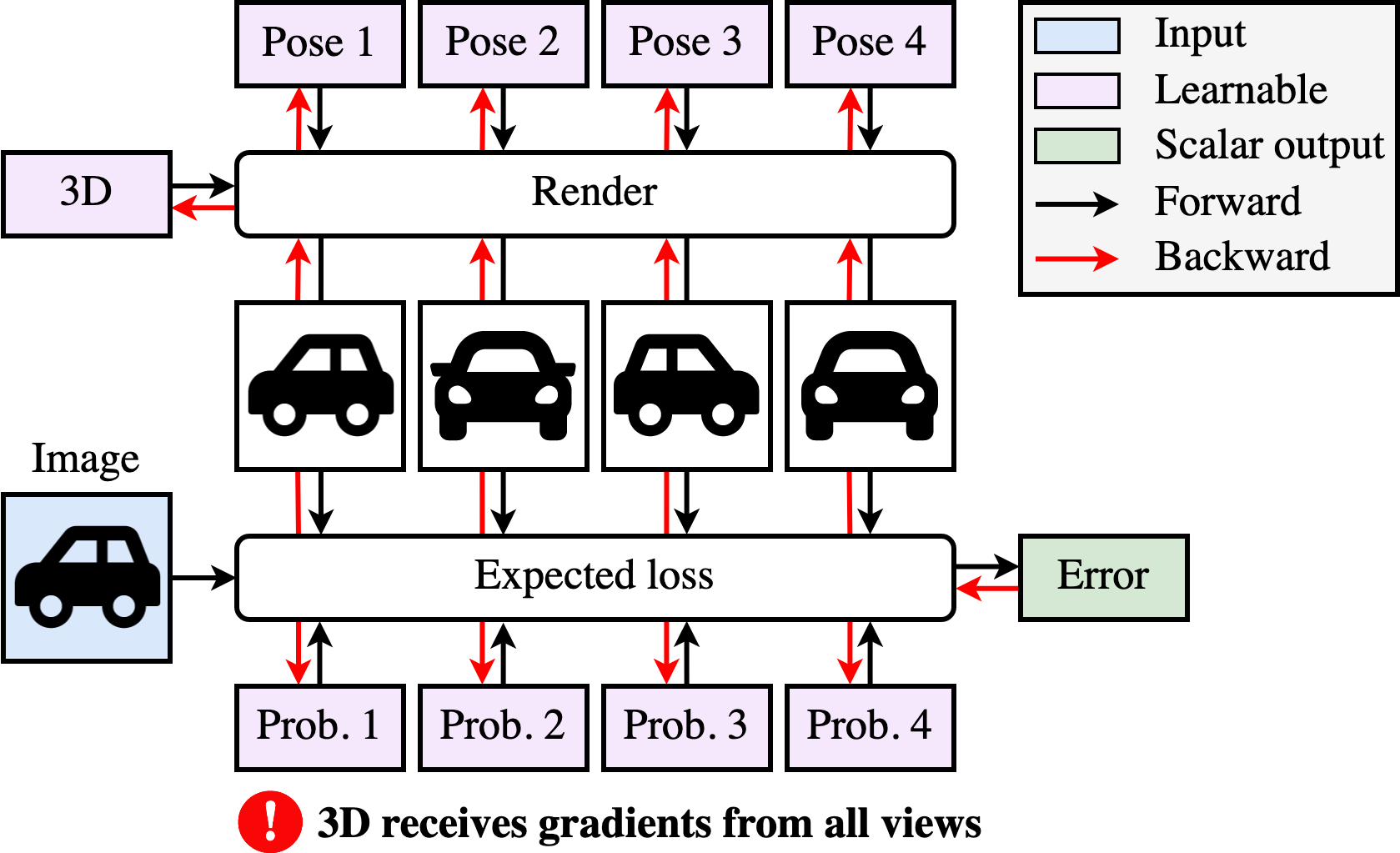
(b) Optimization in [16, 12, 51]

Figure 12: Prior optimizations for joint 3D/pose learning.

In [23], all reconstructions associated to the different pose candidates are computed and both 3D and poses are updated using the reconstruction yielding the minimal error (see Figure 12(a)). We identified two major issues. First, because the other poses are not updated for a given input, we observed that a typical failure case corresponds to a collapse mode where only a single pose (or a small subset of poses) is used for all inputs. Indeed, there is no particular constraint that encourages the use of all pose candidates. Second, inference is not efficient as the object has to be rendered from all poses to find the correct object pose.

In [16, 12, 51], 3D and poses are updated using an expected reconstruction loss (see Figure 12(b)). While this allows to constrain the use of all pose candidates with a regularization on the predicted probabilities, we identified one major weakness common to these frameworks. Because the 3D receives gradients from all views, we observed a typical failure case where the 3D tries to fit the target input from all pose candidates yielding inaccurate texture and geometry. We argue such behaviour was not observed in previous works as they typically use a symmetry prior which prevents it from happening. Note that CMR [12] proposes to directly optimize for each training image a set of parameters corresponding to the pose candidates. This procedure not only involves memory issues as the number of parameters scales linearly with the number of training images, but also inference problems for new images. To mitigate the issue, they propose to use the learned poses as ground-truth to train an additional network that performs pose estimation given a new image.

In contrast, our proposed alternate optimization, illustrated in Figure 13, leverages the best of both worlds: (i) 3D receives gradients from the most likely reconstruction, and (ii) all poses are updated using an expected loss. In practice, we alternate the optimization every new batch of inputs, and we define one iteration as either a a 3D-step or a P-step.

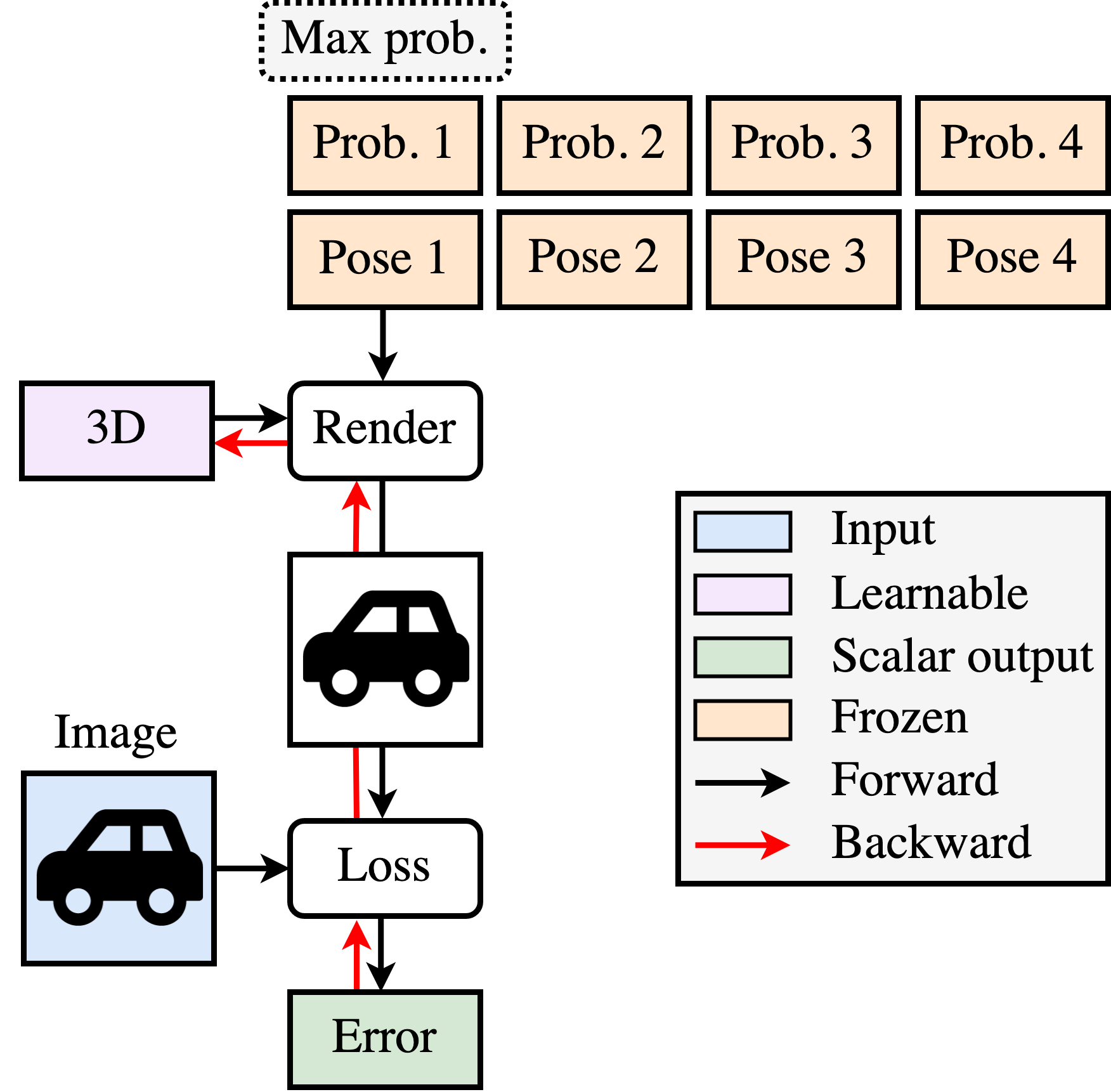
(a) 3D-step

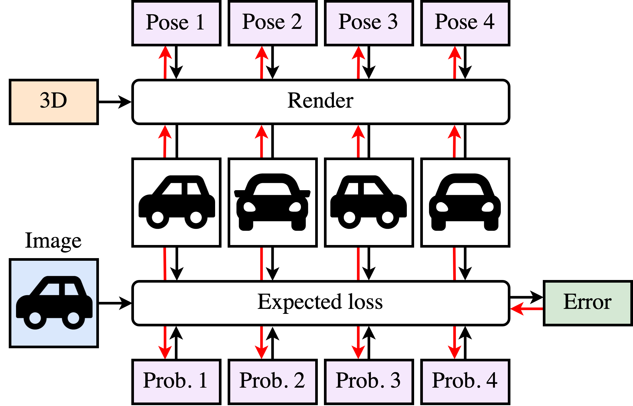
(b) P-step

Figure 13: Our alternate 3D / pose optimization. Compared to prior works, we propose an optimization that alternates between 2 steps. (a) We update the 3D using the most likely pose candidate (3D-step). (b) We update the pose candidates and associated probabilities using the expected loss (P-step).

Appendix 0.C Quantitative evaluation

0.C.1 ICP alignment for better 3D evaluation

In the main paper, we align shapes using our gradient-based version of the Iterative Closest Point (ICP) [3] with anisotropic scaling before evaluating 3D reconstructions. For consistency, we use the same protocol across benchmarks and advocate to do so for future comparisons. First, meshes are centered and normalized so that they exactly fit inside the cube of unit length $[-0.5,0.5]^{3}$; this is important to obtain results that are comparable. Second, we sample 100k points on the mesh surfaces. Third, we run our ICP implementation which minimizes by gradient descent the Chamfer-$L_{2}$ distance between the point clouds by jointly optimizing 3 translation parameters, 6 rotation parameters [68] and 3 scaling parameters. In practice, we use Adam optimizer [31], a learning rate of 0.01 and 100 iterations. Note that we use this gradient-based version of ICP instead of the classical iterative formulation as we found it to diverge when optimizing scale.

We argue that an ICP pre-processing is crucial for an unbiased 3D reconstruction evaluation and provide real examples in Figure 14 to support our claim. Rows correspond to different transformations of the same canonical shape, and for each row, we show: the transformation used, the resulting 3D shape, a rendering example as well as Chamfer-$L_{1}$ distance to the canonical shape. We overlay the visuals with green contours representing the canonical shape and the canonical rendering for easier comparisons. We can make two important observations. First, although all the transformed shapes are excellent 3D reconstructions of the canonical shape, they result in dramatically poor performances. As a comparison, these performances are similar to our ShapeNet results with ICP when the model outputs degenerate reconstructions. Pre-processing the shapes using an ICP with anisotropic scaling mitigates this issue. Second, as shown by the rendering examples, for all these different shapes, we can find a pose that yields almost identical renderings. This hence emphasizes the numerous shape/pose ambiguities that arise from a given rendered image. As a result, it is extremely unlikely that a fully unsupervised SVR system predicting from a single image both the 3D shape and the pose will recover the exact pair of shape/pose used for annotations. In this case, the cameras used for rendering are the same and we do not even consider focal variations, which raises even more ambiguities.

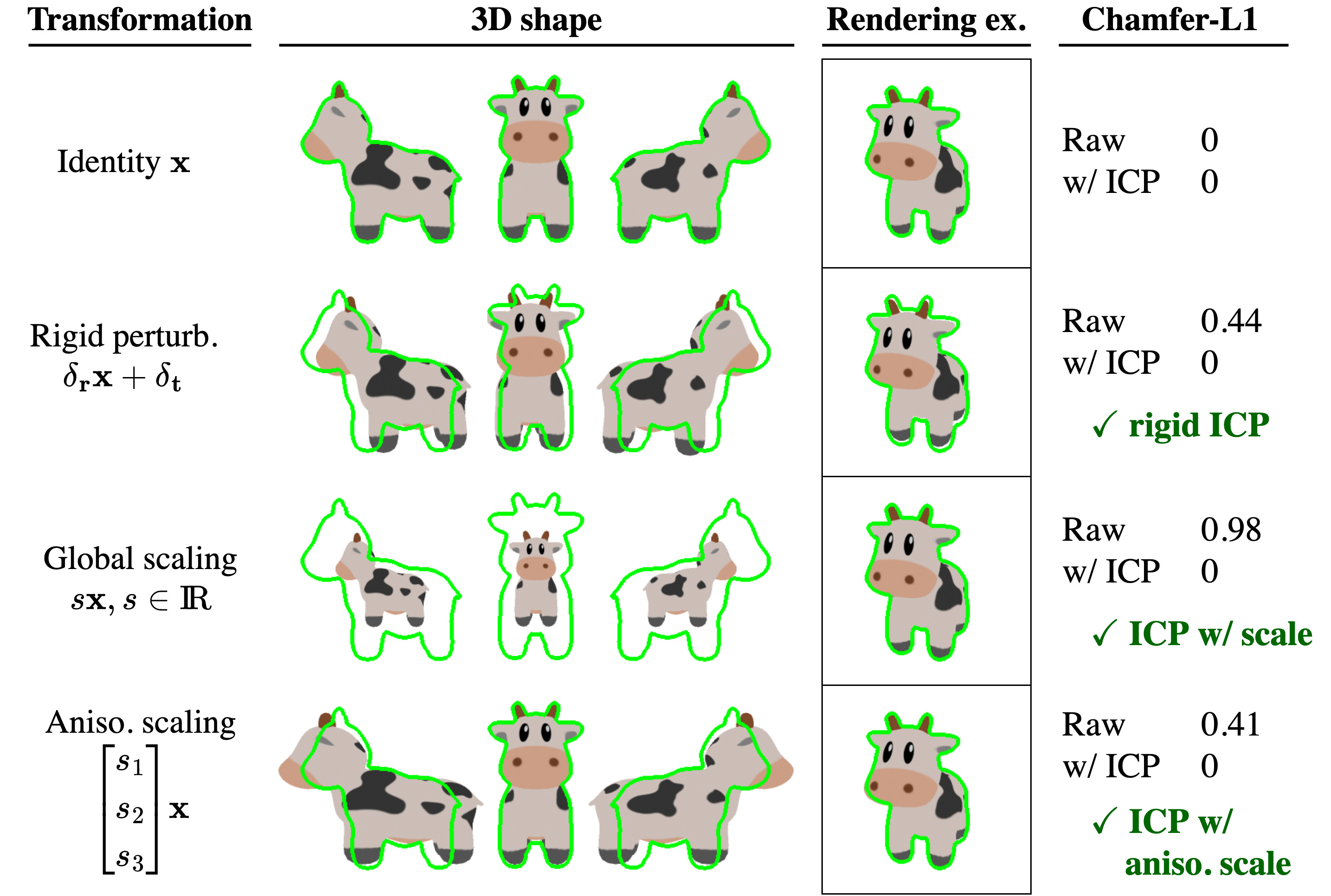
Figure 14: 3D reconstruction evaluation with and without ICP. Rows correspond to results obtained for transformed versions of a canonical shape and columns correspond to, from left to right, the transformation used, resulting 3D shape, a rendering example and Chamfer-$L_{1}$ distance to the canonical shape. Green contours represent the shape and rendering from the canonical object for visual comparisons.

0.C.2 ShapeNet results without ICP

For completeness, we provide quantitative results obtained without ICP on the ShapeNet benchmark in Table 3. We indicate the supervision used and visually separate methods using multi-view supervision. In addition to methods compared in the main paper, we report (i) results from category-agnostic versions (Cat. agn) of DVR [44] and SoftRas [35] presented in [44] and (ii) divergence results obtained by removing silhouette supervision from DVR and SoftRas.

Method	Ours	SDF-SRN	DVR	DVR	SoftRas	DVR	DVR	SoftRas
Cat. agn.							✓	✓
MV				✓	✓	✓	✓	✓
CK		✓	✓	✓	✓	✓	✓	✓
S		✓	✓			✓	✓	✓
airplane	0.186	0.173	0.157	Div.	Div.	0.151	0.190	0.149
bench	0.257	-	0.386	Div.	Div.	0.232	0.210	0.241
cabinet	0.284	-	0.849	Div.	Div.	0.257	0.220	0.231
car	0.251	0.177	0.282	Div.	Div.	0.198	0.196	0.221
chair	0.543	0.333	0.464	Div.	Div.	0.249	0.264	0.338
display	0.344	-	0.968	Div.	Div.	0.281	0.255	0.284
lamp	0.987	-	0.688	Div.	Div.	0.386	0.413	0.381
phone	0.456	-	1.412	Div.	Div.	0.147	0.148	0.131
rifle	0.504	-	0.528	Div.	Div.	0.131	0.175	0.155
sofa	0.335	-	0.665	Div.	Div.	0.218	0.224	0.407
speaker	0.356	-	0.535	Div.	Div.	0.321	0.289	0.320
table	0.351	-	0.442	Div.	Div.	0.283	0.280	0.374
vessel	0.384	-	0.400	Div.	Div.	0.220	0.245	0.233
mean	0.403	-	0.598	Div.	Div.	0.236	0.239	0.266

Table 3: ShapeNet comparison without ICP. We report Chamfer-$L_{1}\downarrow$, supervisions are: Multi-Views, Camera or Keypoints, Silhouettes. We separate methods using multi-views and best results are highlighted in each group.

Appendix 0.D Implementation details

0.D.1 Modeling

0.D.1.1 Network architecture.

We use the same neural network architecture for all experiments. The encoder is composed of 4 CNN backbones followed by separate Multi-Layer Perceptron (MLP) heads predicting a rendering parameter. More specifically, the 4 backbones are respectively used to predict: (i) shape code $\mathbf{z}_{\textrm{sh}}$ and scale $\mathbf{s}$; (ii) texture code $\mathbf{z}_{\textrm{tx}}$; (iii) background code $\mathbf{z}_{\textrm{bg}}$; (iv) rotations $\mathbf{r}_{1:K}$, translations $\mathbf{t}_{1:K}$, and pose probabilities $\mathbf{p}_{1:K}$. Note that using a shared backbone instead of separated ones also yields great results and is advocated for decreasing the memory footprint and training time; the major benefit from using separated backbones is to produce slightly more detailed textures and background. We follow prior works in SVR [14, 37, 44, 12] and use randomly initialized ResNet-18 [15] as backbone. Each MLP head has the same architecture with 3 hidden layers of 128 units and ReLU activations. The last layer of the MLP heads for shape, texture and background codes is initialized to zero to avoid discontinuity when increasing the size of the latent codes. The final activation of the MLP heads for scale, rotation, and translation is a $\tanh$ function and the output is scaled and shifted using predefined constants in order to control their range (see Table 4 for selected ranges). The learnable parts of the decoder are the shape deformation network $s_{\theta}$ and the two CNN generators $t_{\theta}$ and $b_{\theta}$ which respectively output $64\times 64$ images for texture and background. The MLP modeling the deformations has 3 hidden layers, ReLU activations and 128 units for real images; we use an increased number of units for ShapeNet (512) which provides a small boost in performances. The CNN generators share the same architecture which is identical to the generator used in GIRAFFE [43]. We refer the reader to [43] for details.

0.D.1.2 Other design choices.

In all experiments, the predefined anisotropic scaling used to deform the icosphere into an ellipsoid is $[1,0.7,0.7]$. In Table 4, we detail other design choices that are specific to all categories of ShapeNet [4] (second column) or all real-image datasets (third column). This notably includes a predetermined global scaling of the ellipsoid, a camera defined by a focal length $f$ or a field of view (fov), as well as scaling, translation and rotation ranges.

Design type	ShapeNet	Real-image
ellipsoid scale	0.4	0.6
camera	$f=3.732$	$\textrm{fov}=30^{\circ}$
$\mathbf{s}_{x}/\mathbf{s}_{y}/\mathbf{s}_{z}$	$1\pm 0.5$	$1\pm 0.3$
$\mathbf{t}_{x}/\mathbf{t}_{y}$	$0\pm 0.5$	$0\pm 0.3$
$\mathbf{t}_{z}$ (depth)	$2.732$	$2.732\pm 0.3$
$\mathbf{r}_{a}$ (azimuth)	$[0^{\circ},360^{\circ}]$	$[0^{\circ},360^{\circ}]$
$\mathbf{r}_{e}$ (elevation)	$30^{\circ}$	$[-10^{\circ},30^{\circ}]$
$\mathbf{r}_{r}$ (roll)	$0^{\circ}$	$[-30^{\circ},30^{\circ}]$

Table 4: Design choices. Following standard practices [35, 44] on ShapeNet [4], we keep the default rendering values used to generate the images for the focal length $f$, the distance to the camera $\mathbf{t}_{z}$ and the elevation $\mathbf{r}_{e}$. For real images, we keep the classical value of 2.732 for the distance to the camera $\mathbf{t}_{z}$ and use a field of view (fov) of $30^{\circ}$. Note that we did not finetune these parameters, they were selected once through visual comparisons on a toy example.

0.D.2 Training

In all experiments, we use a batch size of 32 images of size $64\times 64$ and Adam optimizer [31] with a constant learning rate of $10^{-4}$ that is divided by 5 at the very end of the training for a few epochs. The training corresponds to 4 stages where latent code dimensions are increased at the beginning of each stage and the network is then trained until convergence. We use dimensions 0/2/8/64 for the shape code, 2/8/64/512 for the texture code, and 4/8/64/256 for the background code if any. In line with the curriculum modeling of [38], we found it beneficial for the first stage to gradually increase the model complexity: we first learn to position the fixed ellipsoid in the image, then we allow the ellipsoid to be deformed, and finally we allow scale variabilities. In particular, we found this procedure prevents the model to learn prototypical shapes with unrealistic proportions. In the following, we describe other training details specific to ShapeNet [4] benchmark and real-image datasets.

0.D.2.1 ShapeNet dataset.

We use the same training strategy for all categories. We train the first stage for 50k iterations, and each of the other stage for 250k iterations, where one iteration corresponds to either a 3D-step or a P-step of our alternate optimization. We do not learn a background model as all images are rendered on top of a white background. However, we found that our system learned in such synthetic setting was prone to a bad local minimum where the predicted textures have white regions that accommodate for wrong shape prediction. Intuitively, this is expected as the system has no particular signal to distinguish white background regions from white object parts. To mitigate the issue, we constrain our texture model as follows: (i) during the first stage, the predicted texture image is averaged to yield a constant texture, and (ii) during the other stages, we occasionally use averaged textures instead of the real ones. More specifically, we sample a Bernoulli variable with probability $p=0.2$ at each iteration and average the predicted texture image in case of success. We found this simple procedure to work well to resolve such shape/texture ambiguity.

0.D.2.2 Real-image datasets.

We use the same training strategy for all real-image datasets. We train each stage for roughly 750k iterations, where one iteration either corresponds to a 3D-step or a P-step of our alternate optimization. Learning our structured autoencoder in such real-image scenario, without silhouette nor symmetry constraints, is very challenging. We found our system sometimes falls into a bad local minimum where the texture model is specialized by viewpoints, e.g., dark cars always correspond to a frontal view and light cars always correspond to a back view. To alleviate the issue, we encourage uniform textures by occasionally using averaged textures instead of the real ones during rendering, as done on the ShapeNet benchmark. More specifically, we sample a Bernoulli variable with probability $p=0.2$ at each iteration and average the predicted texture image in case of success. We observed that it was very effective in practice, and we also found it helped preventing the object texture from modeling background regions. We do not use such technique in the last stage to increase the texture accuracy.

References

- [1] Bengio, S., Vinyals, O., Jaitly, N., Shazeer, N.: Scheduled Sampling for Sequence Prediction with Recurrent Neural Networks. In: NIPS (2015)
- [2] Bengio, Y., Louradour, J., Collobert, R., Weston, J.: Curriculum learning. In: ICML (2009)
- [3] Besl, P., McKay, N.D.: A method for registration of 3-D shapes. TPAMI 14(2) (1992)
- [4] Chang, A.X., Funkhouser, T., Guibas, L., Hanrahan, P., Huang, Q., Li, Z., Savarese, S., Savva, M., Song, S., Su, H., Xiao, J., Yi, L., Yu, F.: ShapeNet: An Information-Rich 3D Model Repository. arXiv:1512.03012 [cs] (2015)
- [5] Chen, W., Gao, J., Ling, H., Smith, E.J., Lehtinen, J., Jacobson, A., Fidler, S.: Learning to Predict 3D Objects with an Interpolation-based Differentiable Renderer. In: NeurIPS (2019)
- [6] Choy, C.B., Xu, D., Gwak, J., Chen, K., Savarese, S.: 3D-R2N2: A Unified Approach for Single and Multi-view 3D Object Reconstruction. In: ECCV (2016)
- [7] Desbrun, M., Meyer, M., Schröder, P., Barr, A.H.: Implicit fairing of irregular meshes using diffusion and curvature flow. In: SIGGRAPH (1999)
- [8] Duggal, S., Pathak, D.: Topologically-Aware Deformation Fields for Single-View 3D Reconstruction. In: CVPR (2022)
- [9] Elman, J.L.: Learning and development in neural networks: The importance of starting small. Cognition (1993)
- [10] Finger, S.: Origins of neuroscience: a history of explorations into brain function. Oxford University Press (1994)
- [11] Gadelha, M., Maji, S., Wang, R.: 3D Shape Induction from 2D Views of Multiple Objects. In: 3DV (2017)
- [12] Goel, S., Kanazawa, A., Malik, J.: Shape and Viewpoint without Keypoints. In: ECCV (2020)
- [13] Goodfellow, I., Pouget-Abadie, J., Mirza, M., Xu, B., Warde-Farley, D., Ozair, S., Courville, A., Bengio, Y.: Generative Adversarial Nets. In: NIPS (2014)
- [14] Groueix, T., Fisher, M., Kim, V.G., Russell, B.C., Aubry, M.: AtlasNet: A Papier-Mâché Approach to Learning 3D Surface Generation. In: CVPR (2018)
- [15] He, K., Zhang, X., Ren, S., Sun, J.: Deep Residual Learning for Image Recognition. In: CVPR (2016)
- [16] Henderson, P., Ferrari, V.: Learning single-image 3D reconstruction by generative modelling of shape, pose and shading. IJCV (2019)
- [17] Henderson, P., Tsiminaki, V., Lampert, C.H.: Leveraging 2D Data to Learn Textured 3D Mesh Generation. In: CVPR (2020)
- [18] Henzler, P., Mitra, N., Ritschel, T.: Escaping Plato’s Cave: 3D Shape From Adversarial Rendering. In: ICCV (2019)
- [19] Hoiem, D., Efros, A.A., Hebert, M.: Geometric Context from a Single Image. In: ICCV (2005)
- [20] Hoiem, D., Efros, A.A., Hebert, M.: Putting Objects in Perspective. IJCV (2008)
- [21] Hu, T., Wang, L., Xu, X., Liu, S., Jia, J.: Self-Supervised 3D Mesh Reconstruction From Single Images. In: CVPR (2021)
- [22] Ilg, E., Mayer, N., Saikia, T., Keuper, M., Dosovitskiy, A., Brox, T.: FlowNet 2.0: Evolution of Optical Flow Estimation with Deep Networks. In: CVPR (2017)
- [23] Insafutdinov, E., Dosovitskiy, A.: Unsupervised Learning of Shape and Pose with Differentiable Point Clouds. In: NIPS (2018)
- [24] Jojic, N., Frey, B.J.: Learning Flexible Sprites in Video Layers. In: CVPR (2001)
- [25] Kanazawa, A., Tulsiani, S., Efros, A.A., Malik, J.: Learning Category-Specific Mesh Reconstruction from Image Collections. In: ECCV (2018)
- [26] Kar, A., Tulsiani, S., Carreira, J., Malik, J.: Category-Specific Object Reconstruction from a Single Image. In: CVPR (2015)
- [27] Karras, T., Laine, S., Aila, T.: A Style-Based Generator Architecture for Generative Adversarial Networks. In: CVPR (2019)
- [28] Kato, H., Beker, D., Morariu, M., Ando, T., Matsuoka, T., Kehl, W., Gaidon, A.: Differentiable Rendering: A Survey. arXiv:2006.12057 [cs] (2020)
- [29] Kato, H., Harada, T.: Learning View Priors for Single-view 3D Reconstruction. In: CVPR (2019)
- [30] Kato, H., Ushiku, Y., Harada, T.: Neural 3D Mesh Renderer. In: CVPR (2018)
- [31] Kingma, D.P., Ba, J.: Adam: A Method for Stochastic Optimization. In: ICLR (2015)
- [32] Kulkarni, N., Gupta, A., Tulsiani, S.: Canonical Surface Mapping via Geometric Cycle Consistency. In: ICCV (2019)
- [33] Li, X., Liu, S., Kim, K., De Mello, S., Jampani, V., Yang, M.H., Kautz, J.: Self-supervised Single-view 3D Reconstruction via Semantic Consistency. In: ECCV (2020)
- [34] Lin, C.H., Wang, C., Lucey, S.: SDF-SRN: Learning Signed Distance 3D Object Reconstruction from Static Images. In: NeurIPS (2020)
- [35] Liu, S., Li, T., Chen, W., Li, H.: Soft Rasterizer: A Differentiable Renderer for Image-based 3D Reasoning. In: ICCV (2019)
- [36] Loper, M.M., Black, M.J.: OpenDR: An Approximate Differentiable Renderer. In: ECCV 2014, vol. 8695 (2014)
- [37] Mescheder, L., Oechsle, M., Niemeyer, M., Nowozin, S., Geiger, A.: Occupancy Networks: Learning 3D Reconstruction in Function Space. In: CVPR (2019)
- [38] Monnier, T., Groueix, T., Aubry, M.: Deep Transformation-Invariant Clustering. In: NeurIPS (2020)
- [39] Monnier, T., Vincent, E., Ponce, J., Aubry, M.: Unsupervised Layered Image Decomposition Into Object Prototypes. In: ICCV (2021)
- [40] Navaneet, K.L., Mathew, A., Kashyap, S., Hung, W.C., Jampani, V., Babu, R.V.: From Image Collections to Point Clouds with Self-supervised Shape and Pose Networks. In: CVPR (2020)
- [41] Nealen, A., Igarashi, T., Sorkine, O., Alexa, M.: Laplacian mesh optimization. In: GRAPHITE (2006)
- [42] Nguyen-Phuoc, T., Li, C., Theis, L., Richardt, C., Yang, Y.L.: HoloGAN: Unsupervised learning of 3D representations from natural images. In: ICCV (2019)
- [43] Niemeyer, M., Geiger, A.: GIRAFFE: Representing Scenes as Compositional Generative Neural Feature Fields. In: CVPR (2021)
- [44] Niemeyer, M., Mescheder, L., Oechsle, M., Geiger, A.: Differentiable Volumetric Rendering: Learning Implicit 3D Representations without 3D Supervision. In: CVPR (2020)
- [45] Pavllo, D., Spinks, G., Hofmann, T., Moens, M.F., Lucchi, A.: Convolutional Generation of Textured 3D Meshes. In: NeurIPS (2020)
- [46] Ravi, N., Reizenstein, J., Novotny, D., Gordon, T., Lo, W.Y., Johnson, J., Gkioxari, G.: Accelerating 3D Deep Learning with PyTorch3D. arXiv:2007.08501 [cs] (2020)
- [47] Saxena, A., Min Sun, Ng, A.: Make3D: Learning 3D Scene Structure from a Single Still Image. TPAMI (2009)
- [48] Schroff, F., Kalenichenko, D., Philbin, J.: FaceNet: A unified embedding for face recognition and clustering. In: CVPR (2015)
- [49] Simonyan, K., Zisserman, A.: Very Deep Convolutional Networks for Large-Scale Image Recognition. In: ICLR (2015)
- [50] Tulsiani, S., Efros, A.A., Malik, J.: Multi-view Consistency as Supervisory Signal for Learning Shape and Pose Prediction. In: CVPR (2018)
- [51] Tulsiani, S., Kulkarni, N., Gupta, A.: Implicit Mesh Reconstruction from Unannotated Image Collections. arXiv:2007.08504 [cs] (2020)
- [52] Tulsiani, S., Zhou, T., Efros, A.A., Malik, J.: Multi-view Supervision for Single-view Reconstruction via Differentiable Ray Consistency. In: CVPR (2017)
- [53] Vicente, S., Carreira, J., Agapito, L., Batista, J.: Reconstructing PASCAL VOC. In: CVPR (2014)
- [54] Wang, N., Zhang, Y., Li, Z., Fu, Y., Liu, W., Jiang, Y.G.: Pixel2Mesh: Generating 3D Mesh Models from Single RGB Images. In: ECCV (2018)
- [55] Welinder, P., Branson, S., Mita, T., Wah, C., Schroff, F., Belongie, S., Perona, P.: Caltech-UCSD Birds 200. Tech. rep., California Institute of Technology (2010)
- [56] Wu, S., Makadia, A., Wu, J., Snavely, N., Tucker, R., Kanazawa, A.: De-rendering the World’s Revolutionary Artefacts. In: CVPR (2021)
- [57] Wu, S., Rupprecht, C., Vedaldi, A.: Unsupervised Learning of Probably Symmetric Deformable 3D Objects from Images in the Wild. In: CVPR (2020)
- [58] Xiang, Y., Mottaghi, R., Savarese, S.: Beyond PASCAL: A benchmark for 3D object detection in the wild. In: WACV (2014)
- [59] Xu, Q., Wang, W., Ceylan, D., Mech, R., Neumann, U.: DISN: Deep Implicit Surface Network for High-quality Single-view 3D Reconstruction. In: NeurIPS (2019)
- [60] Yan, X., Yang, J., Yumer, E., Guo, Y., Lee, H.: Perspective Transformer Nets: Learning Single-View 3D Object Reconstruction without 3D Supervision. In: NeurIPS (2016)
- [61] Yang, L., Luo, P., Loy, C.C., Tang, X.: A large-scale car dataset for fine-grained categorization and verification. In: CVPR (2015)
- [62] Yao, C.H., Hung, W.C., Jampani, V., Yang, M.H.: Discovering 3D Parts from Image Collections. In: ICCV (2021)
- [63] Ye, Y., Tulsiani, S., Gupta, A.: Shelf-Supervised Mesh Prediction in the Wild. arXiv:2102.06195 [cs] (2021)
- [64] Yu, F., Seff, A., Zhang, Y., Song, S., Funkhouser, T., Xiao, J.: LSUN: Construction of a Large-scale Image Dataset using Deep Learning with Humans in the Loop. arXiv:1506.03365 [cs] (2016)
- [65] Zhang, J.Y., Yang, G., Tulsiani, S., Ramanan, D.: NeRS: Neural Reflectance Surfaces for Sparse-view 3D Reconstruction in the Wild. In: NeurIPS (2021)
- [66] Zhang, R., Isola, P., Efros, A.A., Shechtman, E., Wang, O.: The Unreasonable Effectiveness of Deep Features as a Perceptual Metric. In: CVPR (2018)
- [67] Zhang, Y., Chen, W., Ling, H., Gao, J., Zhang, Y., Torralba, A., Fidler, S.: Image GANs meet Differentiable Rendering for Inverse Graphics and Interpretable 3D Neural Rendering. In: ICLR (2021)
- [68] Zhou, Y., Barnes, C., Lu, J., Yang, J., Li, H.: On the Continuity of Rotation Representations in Neural Networks. In: CVPR (2020)