Structural Nested Mean Models Under Parallel Trends Assumptions

Zach Shahn CUNY School of Public Health, New York, NY, USA IBM Research, Yorktown Heights, NY, USA Oliver Dukes University of Pennsylvania, Philadelphia, PA, USA David Richardson University of California Irvine, Irvine, CA, USA Eric Tchetgen Tchetgen University of Pennsylvania, Philadelphia, PA, USA James Robins Harvard TH Chan School of Public Health, Boston, MA, USA
(May, 2022)

Abstract

In this paper, we generalize methods in the Difference in Differences (DiD) literature by showing that both additive and multiplicative standard and coarse Structural Nested Mean Models (Robins, 1994, 1997, 1998, 2000, 2004; Lok and Degruttola, 2012; Vansteelandt and Joffe, 2014) are identified under parallel trends assumptions. Our methodology enables adjustment for time-varying covariates, identification of effect heterogeneity as a function of time-varying covariates, identification of additional causal contrasts (such as effects of a ‘blip’ of treatment at a single time point followed by no further treatment and controlled direct effects), and estimation of treatment effects under a general class of treatment patterns (e.g. we do not restrict to the ‘staggered adoption’ setting, and treatments can be multidimensional with any mix of categorical and continuous components). We stress that these extensions come essentially for free, as our parallel trends assumption is not stronger than other parallel trends assumptions in the DiD literature. We also provide a method for sensitivity analysis to violations of our parallel trends assumption. However, in contrast to much of the DiD literature, we only consider panel data, not repeated cross sectional data. We also explain how to estimate optimal treatment regimes via optimal regime Structural Nested Mean Models under parallel trends assumptions plus an assumption that there is no effect modification by unobserved confounders. Finally, we illustrate our methods with real data applications estimating effects of bank deregulation on housing prices and effects of floods on flood insurance take-up.

1 Introduction

The Difference in Differences (DiD) design (Snow, 1855; Card and Krueger, 1993) is a popular approach to estimating causal effects in the possible presence of unobserved confounding. The key assumption it requires is ‘parallel trends’, i.e. the average trend in counterfactual untreated outcomes is equal among the treated and the untreated. The canonical DiD design identifies effects of treatments delivered at a single time period, but recently there has been a significant literature (e.g. Roth et al., 2022; Callaway and Sant’Anna, 2021; Chaisemartin and D’Haultfoeuille, 2021; Athey and Imbens, 2018; Bojinov et al, 2020) on extensions to time-varying treatment strategies. Under a time-varying version of the parallel trends assumption (possibly conditional on baseline covariates), Callaway and Sant’Anna (2021) nonparametrically identify treatment effects under ‘staggered adoption’ strategies. That is, for times $k>m$, they identify the effect of starting treatment at time $m$ compared to never starting treatment on the outcome at time $k$ among those who actually started treatment at time $m$. In addition, they identify effect heterogeneity by baseline covariates.

We extend this work in several ways. We introduce a parallel trends assumption conditional on time-varying covariates that generalizes the parallel trends assumption of Callaway and Sant’Anna (2021), which is conditional only on baseline covariates. Under our conditional time-varying parallel trends assumption, we show that it is possible to identify the parameters of a standard Structural Nested Mean Model (SNMM) (Robins, 1994, 1997, 2000, 2004; Vansteelandt and Joffe, 2014) or a coarse SNMM (Robins, 1998; Lok and DeGruttola, 2012). A standard SNMM is a model for the conditional effect of one last ‘blip’ of treatment delivered at time $m$ followed by no treatment thereafter compared to no treatment from time $m$ onward conditional on previous treatment and covariate history. A coarse SNMM (Robins, 1998; Lok and DeGruttola, 2012) models the conditional effect of initiating treatment for the first time at time $m$ compared to never initiating treatment given covariate history through $m$ in those who actually initiated treatment at time $m$. (We will give a more formal review of standard and coarse SNMMs later. Coarse SNMMs are particularly important in staggered adoption settings because interest centers entirely on the effect of treatment initiation and the positivity assumptions needed for standard SNMMs are not satisfied. In settings where subjects go off and on treatment, coarse SNMMs can be used to model intention-to-treat effects of initial departures from the baseline treatment level marginalized over future treatment patterns under the observational regime. Such intention-to-treat effects are similar to those considered by Chaisemartin and D’Haultfoeuille (2021).) SNMMs are thus powerful models for effect heterogeneity as a function of time-varying covariates, and many counterfactual quantities and causal contrasts beyond conditional effects of treatment on the treated described above can be identified in terms of their parameters (including, as we show in Section 8, controlled direct effects (Robins and Greenland, 1992)). SNMMs can also model effects of multidimensional treatments with continuous and discrete components. Past work has shown that SNMM parameters can be consistently estimated via ‘g-estimation’ under no unobserved confounding assumptions (Robins, 1994, 1997, 1998, 2004). Here, we show that SNMM parameters are also identified under a time-varying conditional parallel trends assumption: conditional on observed history through time $m$, untreated counterfactual outcome trajectories from time $m$ onwards are parallel in the treated and untreated for all $m$.

The extensions enabled by identification of SNMMs under parallel trends come essentially for free, in the sense that our parallel trends assumption is not stronger than other parallel trends assumptions in the time-varying DiD literature. In fact, our conditional time-varying parallel trends assumption might be considered more plausible than an assumption that conditions only on baseline covariates. For example, if treatment and trends in counterfactual outcomes are both associated with a time-varying covariate, then the baseline version of the parallel trends assumption would not hold, but parallel trends conditional on that time-varying covariate might hold. Thus, our parallel trends assumption is a generalization that allows identification in some additional settings compared to previous methods. However, in this paper we do assume throughout that panel data are available. We note that this differs from many DiD applications that use repeated cross sectional data with different subjects in each cross section.

The organization of the paper is as follows. In Section 2, we establish notation, assumptions, and review SNMMs. In Section 3, we identify and provide a doubly robust estimator for the parameters of a coarse SNMM under our parallel trends assumption. In Section 4, we identify and provide a doubly robust estimator of standard SNMM parameters under our parallel trends assumption. In Section 5, we consider SNMMs for multiplicative effects. In Section 6, we explain how to estimate the parameters of general regime SNMMs under a parallel trends assumption and how to estimate the optimal regime via an optimal regime SNMM under parallel trends assumptions plus an additional no effect modification by unobserved confounders assumption. In Section 7, we present two applications to real data, a coarse SNMM of effects of bank deregulation on housing prices and a standard SNMM of effects of floods on flood insurance take-up. In Section 8, we discuss some extensions, including descriptions of how to estimate controlled direct effects and perform sensitivity analysis for violations of conditional parallel trends. The theme of the paper is that it is fruitful to use structural nested mean models under DiD assumptions.

2 Notation, Assumptions, and SNMMs

Suppose we observe a cohort of $N$ subjects indexed by $i\in\{1,\ldots,N\}$. Assume that each subject is observed at regular intervals from baseline time 00 through end of followup time $K$, and there is no loss to follow-up. At each time point $m$, the data are collected on $\mathbbm{O}_{m}=(Z_{m},Y_{m},A_{m})$ in that temporal order. $A_{m}$ denotes the (possibly multidimensional with discrete and/or continuous components) treatment received at time $m$, $Y_{m}$ denotes the outcome of interest at time $m$, and $Z_{m}$ denotes a vector of covariates at time $m$ excluding $Y_{m}$. Hence $Z_{0}$ constitutes the vector of baseline covariates other than $Y_{0}$. For arbitrary time varying variable $X$: we denote by $\bar{X}_{m}=(X_{0},\ldots,X_{m})$ the history of $X$ through time $m$; we denote by $\underline{X}_{m}=(X_{m},\ldots,X_{K})$ the future of $X$ from time $m$ through time $K$; and whenever the negative index $X_{-1}$ appears it denotes the null value with probability 1. Define $\bar{L}_{m}$ to be $(\bar{Z}_{m},\bar{Y}_{m-1},\bar{A}_{m-1})$, the history through time $m$ excluding $(Y_{m},A_{m})$. Hence $L_{0}$ is $Z_{0}$. We adopt the counterfactual framework for time-varying treatments (Robins, 1986) which posits that corresponding to each time-varying treatment regime $\bar{a}_{m}$, each subject has a counterfactual or potential outcome $Y_{m+1}(\bar{a}_{m})$ that would have been observed had that subject received treatment regime $\bar{a}_{m}$.

Throughout, we make the assumption

$$\textbf{Consistency: }Y_{m}(\bar{A}_{m-1})=Y_{m}\text{ }\forall m\leq K$$ (1)

stating that observed outcomes are equal to counterfactual outcomes corresponding to observed treatments. This assumption is necessary to link observed data to the counterfactual data.

We will use slightly different notation and make different assumptions for coarse and standard SNMMs. Coarse SNMMs specifically model effects of initial deviations from a baseline treatment level. Standard SNMMs model the effect of a final blip of treatment at occasion $m$ followed by the baseline level of treatment thereafter. The staggered adoption setting where treatment is sustained once initiated is an important setting in the DiD literature where coarse SNMMs are required. In other settings, both coarse and standard SNMMs might be used. We will describe notation and assumptions for coarse and standard SNMMs in separate subsections below. Throughout, we code treatment such that at time $m$, 00 denotes the baseline level of treatment at at that time.

2.1 Standard SNMMs

Whenever discussing standard SNMMs, we will assume

$$\textbf{Positivity: }f_{A_{m}|\bar{L}_{m},\bar{A}_{m-1}}(0|\bar{l}_{m},\bar{a}_{m-1})>0\text{ whenever }f_{\bar{L}_{m},\bar{A}_{m-1}}(\bar{l}_{m},\bar{a}_{m-1})>0.$$ (2)

However, we note that under parametric versions of the models we consider positivity is not strictly necessary. Note that this positivity assumption excludes the staggered adoption setting where $f_{A_{m}|\bar{L}_{m},\bar{A}_{m-1}}(0|\bar{l}_{m},\bar{a}_{m-1})=0$ if $a_{m-1}\neq 0$.

Define the causal contrasts

$$\gamma_{mk}^{*}(\bar{l}_{m},\bar{a}_{m})\equiv E[Y_{k}(\bar{a}_{m},\underline{0})-Y_{k}(\bar{a}_{m-1},\underline{0})|\bar{A}_{m}=\bar{a}_{m},\bar{L}_{m}=\bar{l}_{m}]$$ (3)

for all $k>m$. $\gamma_{mk}^{*}(\bar{a}_{m},\bar{l}_{m})$ is the average effect at time $k$ among patients with history $(\bar{A}_{m}=\bar{a}_{m},\bar{L}_{m}=\bar{l}_{m})$ of receiving treatment $a_{m}$ at time $m$ and then 00 thereafter compared to receiving treatment 00 at time $m$ and thereafter. (Here ‘0’ can be replaced by any baseline value $a_{m}^{*}$.) These contrasts are sometimes called ‘blip functions’ because they are the effects of one last blip of treatment. Note $\gamma_{mk}^{\ast}(\bar{l}_{m},\bar{a}_{m})=0$ if a${}_{m}=0$.

A parametric standard SNMM imposes functional forms on the blip functions $\gamma^{*}_{mk}(\bar{A}_{m},\bar{L}_{m})$ for each $k>m$, i.e.

$$\gamma^{*}_{mk}(\bar{a}_{m},\bar{l}_{m})=\gamma_{mk}(\bar{a}_{m},\bar{l}_{m};\psi^{*}),$$ (4)

where $\psi^{*}$ is an unknown finite dimensional parameter vector and $\gamma_{mk}(\bar{a}_{m},\bar{l}_{m};\psi)$ is a known function equal to 00 whenever $\psi=0$ or $a_{m}=0$.

From a policy perspective, our motivation to fit a standard SNMM is typically that were the $\gamma_{mk}^{*}(\bar{a}_{m},\bar{l}_{m})$ (i.e. $\psi^{*}$ under (4)) identified, then for any subject history $(\bar{L}_{m}=\bar{l}_{m},\bar{A}_{m}=\bar{a}_{m-1})$ of interest, the expected conditional counterfactual outcome trajectory under no further treatment, i.e. $E[\underline{Y}_{m}(a_{m-1},\underline{0})|\bar{L}_{m}=\bar{l}_{m},\bar{A}_{m-1}=\bar{a}_{m-1}]$, would also be identified. We could also identify quantities that further condition on treatment at $m$, i.e. $E[\underline{Y}_{m}(a_{m-1},\underline{0})|\bar{L}_{m}=\bar{l}_{m},\bar{A}_{m}=\bar{a}_{m}]$. Or we could marginalize over $\bar{L}_{m}$ to identify $E[\underline{Y}_{m}(a_{m-1},\underline{0})|\bar{A}_{m-1}=\bar{a}_{m-1}]$ and $E[\underline{Y}_{m}(a_{m-1},\underline{0})|\bar{A}_{m}=\bar{a}_{m}]$. The derived quantity $E[\bar{Y}_{K}(\bar{0})]$, i.e. the expected counterfactual trajectory under no treatment, would also be identified. From a scientific perspective, the goal might be to determine the subset of $(\bar{L}_{m},\bar{A}_{m-1})$ that are time dependent effect modifiers of the causal contrast (3).

Robins (1994, 1997, 2004) has shown that $\gamma^{*}=(\gamma^{*}_{01},\ldots,\gamma^{*}_{(K-1)K})$, the vector of all functions $\gamma^{*}_{mk}=\gamma^{*}_{mk}(\bar{a}_{m},\bar{l}_{m})$ with $m<k\leq K$, is identified and how to consistently estimate $\psi^{*}$ under the assumption that there are no unobserved confounders, i.e.

$$Y_{k}(\bar{a}_{m-1},\underline{0})\mathchoice{\mathrel{\hbox to0.0pt{$\displaystyle\perp$\hss}\mkern 2.0mu{\displaystyle\perp}}}{\mathrel{\hbox to0.0pt{$\textstyle\perp$\hss}\mkern 2.0mu{\textstyle\perp}}}{\mathrel{\hbox to0.0pt{$\scriptstyle\perp$\hss}\mkern 2.0mu{\scriptstyle\perp}}}{\mathrel{\hbox to0.0pt{$\scriptscriptstyle\perp$\hss}\mkern 2.0mu{\scriptscriptstyle\perp}}}A_{m}|\bar{A}_{m-1}=\bar{a}_{m-1},\bar{L}_{m}\text{ }\forall k>m,\bar{a}_{m-1}.$$

In the DiD setting, we will instead make the parallel trends assumption

$\displaystyle\begin{split}&\textbf{Time-Varying Conditional Parallel Trends: }\\ &E[Y_{k}(\bar{a}_{m-1},\underline{0})-Y_{k-1}(\bar{a}_{m-1},\underline{0})|\bar{A}_{m}=\bar{a}_{m},\bar{L}_{m}]=\\ &E[Y_{k}(\bar{a}_{m-1},\underline{0})-Y_{k-1}(\bar{a}_{m-1},\underline{0})|\bar{A}_{m}=(\bar{a}_{m-1},0),\bar{L}_{m}]\\ &\forall k>m.\end{split}$ (5)

When $k=m+1$, this assumption reduces to

$$E[Y_{m+1}(\bar{a}_{m-1},0)-Y_{m}|\bar{A}_{m}=\bar{a}_{m},\bar{L}_{m}]=E[Y_{m+1}(\bar{a}_{m-1},0)-Y_{m}|\bar{A}_{m}=(\bar{a}_{m-1},0),\bar{L}_{m}].$$ (6)

The time-varying conditional parallel trends assumption states that, conditional on observed covariate history through time $m$ and treatment history through time $m-1$, the expected counterfactual outcome trends setting treatment to 0 from time $m$ onwards do not depend on the treatment actually received at time $m$. (LABEL:parallel_trends) will often be a more plausible assumption than a version that does not condition on time-varying covariates. If $\bar{L}_{m}$ is associated with both $A_{m}$ and counterfactual outcome trends, then (LABEL:parallel_trends) may hold but an assumption that does not condition on $\bar{L}_{m}$ would not.

Remark 1.

Note that we have defined $\bar{L}_{m}$ to not include $Y_{m}$, since if it did then when $k=m+1$ the parallel trends assumption would imply that there is no unobserved confounding, which we do not wish to assume as then DiD estimators would not be needed. This means we cannot adjust for the most recent outcome or estimate effect heterogeneity conditional on the most recent outcome. However, $\bar{Y}_{m-1}$ is included in $\bar{L}_{m}$.

2.2 Coarse SNMMs

If we are only interested in the effects of first treatment initiation (where we use the term ‘treatment initiation’ to refer to the first departure from the baseline treatment level of 00), then let $T\in\{0,\ldots,K,\infty\}$ denote time of treatment initiation with $\infty$ denoting the strategy of never initiating treatment. Let $Y_{k}(m,a_{m})$ denote the counterfactual outcome at time $k>m$ under the strategy that initiates treatment at value $a_{m}$ at time $m$, with $Y(\infty)$ denoting the counterfactual outcome at time $k$ under the strategy that never initiates treatment. Note $Y_{k}(\infty)=Y_{k}(m,a_{m})$ for $k\leq m$. An important setting where treatment initiation effects are of sole interest is the staggered adoption setting where $A_{m}=a_{m}$ implies that $A_{k}=a_{m}$ for all $k\geq m$. However, we discuss examples where coarse SNMMs might still be useful even if arbitrary treatment patterns are found in the data.

For coarse SNMM identification, we make a weaker positivity assumption that only holds when treatment has not yet been initiated.

$$\textbf{Coarse Positivity: }f_{A_{m}|\bar{L}_{m},T\geq m}(a_{m}|\bar{l}_{m},T\geq m)>0\text{ whenever }f_{\bar{L}_{m},\bar{A}_{m-1}}(\bar{l}_{m},T\geq m)>0.$$ (7)

Interest centers on the causal contrasts

$$\gamma^{c*}_{mk}(\bar{l}_{m},a_{m})\equiv E[Y_{k}(m,a_{m})-Y_{k}(\infty)|T=m,A_{m}=a_{m},\bar{L}_{m}=\bar{l}_{m}]$$ (8)

for all $k>m$. These contrasts are conditional treatment effects on the treated of initial departures from baseline treatment levels.

A parametric coarse SNMM imposes functional forms on $\gamma_{mk}^{c*}(\bar{l}_{m},a_{m})$ for each $k\geq m$, i.e.

$$\gamma_{mk}^{c*}(\bar{l}_{m},a_{m})=\gamma_{mk}^{c}(\bar{l}_{m},a_{m};\psi^{*}_{c})$$ (9)

where $\psi^{*}_{c}$ is an unknown finite dimensional parameter vector and $\gamma^{c}_{mk}(\bar{l}_{m},a_{m};\psi_{c})$ is a known function equal to 00 whenever $\psi_{c}=0$.

As in the case of standard SNMMs, additional derived quantities of interest become identified along with the $\gamma_{mk}^{c*}(\bar{l}_{m},a_{m})$ (i.e. $\psi^{*}_{c}$ under (9)). For instance, the expected counterfactual trajectory under no treatment ($E[\bar{Y}_{K}(\infty)]$), the expected counterfactual trajectory under no treatment in the treated ($E[\underline{Y}_{m+1}(\infty)|T=m,A_{m}=a_{m}]$) would also be identified.

To identify $\gamma^{c*}=(\gamma^{c*}_{01},\ldots,\gamma^{c*}_{(K-1)K})$, the vector of all functions $\gamma^{c*}_{mk}(\bar{l}_{m},a_{m})$ with $m<k\leq K$, we make the coarse time-varying conditional parallel trends assumption that

$\displaystyle\begin{split}&\textbf{Coarse Time-Varying Conditional Parallel Trends: }\\ &E[Y_{k}(\infty)-Y_{k-1}(\infty)|T=m,A_{m},\bar{L}_{m}]=E[Y_{k}(\infty)-Y_{k-1}(\infty)|T>m,\bar{L}_{m}]\forall k>m.\end{split}$ (10)

An implication of (LABEL:coarse_parallel) is that

$$E[Y_{k}(\infty)-Y_{k-1}(\infty)|T\geq m,A_{m}=a_{m},\bar{L}_{m}=\bar{l}_{m}]$$ (11)

does not depend on $a_{m}$. In words, conditional on observed covariate history through time $m$, the expected untreated counterfactual outcome trends from time $m$ onwards are the same in those who initiate treatment (at any value) at time $m$ and those who do not yet initiate treatment at time $m$. Note that our definition of $\bar{L}_{m}$ implies that we do not condition on $Y_{m}$ in (8) or (LABEL:coarse_parallel).

3 Identification and g-Estimation of Coarse SNMMs under Parallel Trends

Because much of the DiD literature deals with the staggered adoption setting, where the positivity assumption is only satisfied for coarse SNMMs, we will discuss identification and estimation of coarse SNMMs first.

3.1 Identification

For any $\gamma^{c}$ a vector of functions $\gamma^{c}_{mk}(\bar{l}_{m},a_{m})$ ranging over $K\geq k>m$, let

$$H^{c}_{mk}(\gamma^{c})\equiv Y_{k}-\sum_{j=m}^{k-1}\gamma^{c}_{jk}(\bar{L}_{j},A_{j})\mathbbm{1}\{T=j\}\text{ for }k>m\text{ and }H^{c}_{mm}(\gamma^{c})\equiv Y_{m}.$$ (12)

$H^{c}_{mk}(\gamma^{c*})$ has the following important properties (Robins, 1998) for all $k>m$:

$\displaystyle\begin{split}&E[H_{mk}^{c}(\gamma^{c*})|\bar{L}_{m},T\geq m,A_{m}]=E[Y_{k}(\infty)|\bar{L}_{m},T\geq m,A_{m}]\\ &E[H_{0k}^{c}(\gamma^{c*})]=E[Y_{k}(\infty)].\end{split}$ (13)

From (LABEL:coarse_H_cf) and the coarse time-varying conditional parallel trends assumption (LABEL:coarse_parallel) it follows that

$\displaystyle\begin{split}&E[H^{c}_{mk}(\gamma^{c*})-H^{c}_{mk-1}(\gamma^{c*})|T\geq m,A_{m}=a_{m},\bar{L}_{m}]=\\ &E[H^{c}_{mk}(\gamma^{c*})-H^{c}_{mk-1}(\gamma^{c*})|T>m,\bar{L}_{m}]\text{ }\forall k>m.\end{split}$ (14)

Note that the quantity $H^{c}_{mk}(\gamma^{c*})$ behaves like the counterfactual quantity $Y_{k}(\infty)$ in that its conditional trend in those not treated prior to time $m$ does not depend on $A_{m}$. We can exploit this property to identify and construct doubly robust estimating equations for $\gamma^{c*}$ and other quantities of interest.

Theorem 1.

Under (1), (7), and (LABEL:coarse_parallel),
(i) $\mathbf{\gamma}^{c*}$ is identified from the joint distribution of $O=(\bar{L}_{K},\overline{A}_{K})$ as the unique solution to

$$E\left[\sum_{K\geq k>m}U^{c}_{mk}(s_{m},\mathbf{\gamma}^{c})\right]=0$$ (15)

where

$\displaystyle U_{mk}^{c}(s_{m},\mathbf{\gamma}^{c})$ $\displaystyle=\mathbbm{1}\{T\geq m\}\{H_{mk}^{c}(\mathbf{\gamma}^{c})-H_{m\left(k-1\right)}^{c}(\mathbf{\gamma}^{c})\}\times$
$\displaystyle\{s_{m}(k,\overline{L}_{m},A_{m})-E\left[s_{m}(k,\overline{L}_{m},A_{m})|\overline{L}_{m},T\geq m\right]\}$

as $s_{m}(k,\overline{l}_{m},a_{m})$ varies over all functions of $k,\overline{l}_{m},a_{m}$. (If $A_{m}$ are Bernoulli then the last expression is $s_{m}(k,\overline{L}_{m},a_{m}=1)\{A_{m}-E[A_{m}|\overline{L}_{m},T\geq m]\}.$)


(ii) $\gamma^{c*}$ satisfies the estimating function

$$E[\sum_{K\geq k>m}\sum_{m=0}^{K-1}U^{c\dagger}_{mk}(s_{m},\mathbf{\gamma}^{c*},\widetilde{v}_{m}^{c},\widetilde{E}_{A_{m}|\overline{L}_{m},T\geq m})]=0$$ (16)

with

$\displaystyle U^{c\dagger}_{mk}(s_{m},\mathbf{\gamma}^{c*},\widetilde{v}_{m}^{c},\widetilde{E}_{A_{m}|\overline{l}_{m},T\geq m})=\mathbbm{1}\{T\geq m\}\{H^{c}_{mk}(\mathbf{\gamma}^{c*})-H_{m(k-1)}(\mathbf{\gamma}^{c*})-\widetilde{v}_{m}(k,\overline{L}_{m})\}\times$
$\displaystyle\{s_{m}(k,\overline{L}_{m},A_{m})-\widetilde{E}_{A_{m}|\overline{L}_{m},T\geq m}[s_{m}(k,\overline{L}_{m},A_{m})|\overline{L}_{m},T\geq m]\}$

for any $s_{m}(k,\overline{l}_{m},a_{m})$ if either

(a) $\widetilde{v}_{m}^{c}(k,\overline{l}_{m})=v_{m}^{c}(k,\overline{l}_{m};\gamma^{c*})$ for all $k>m$, where

$$v_{m}^{c}(k,\overline{l}_{m};\gamma^{c})\equiv E[H^{c}_{mk}(\gamma^{c})-H^{c}_{mk-1}(\gamma^{c})|\bar{L}_{m},T\geq m]$$

or

(b) $\widetilde{E}_{A_{m}|\overline{L}_{m},T\geq m}=E_{A_{m}|\overline{L}_{m},T\geq m}$ for all m.

(16) is thus a doubly robust estimating function.

Proof.

See Appendix A. ∎

It is of course an immediate corollary of Theorem 1 that quantities derived from $\gamma^{c*}$, such as $E[\bar{Y}_{K}(\infty)]$ and $E[\underline{Y}_{m+1}(\infty)|T=m,A_{m}=a_{m}]$ discussed in Section 2.2, are also identified.

3.2 Estimation

Theorem 1 establishes nonparametric identification of time-varying heterogeneous effects modeled by a coarse SNMM under a parallel trends assumption conditional on time-varying covariates. Estimation would often proceed by first specifying a model (9) with finite dimensional parameter $\psi_{c}^{\ast}$. It follows from the doubly robust estimating equations in Theorem 1 and arguments in Chernozhukov et al. (2018) and Smucler et al. (2019) that under regularity conditions we can obtain a consistent asymptotically normal estimator of $\psi_{c}^{\ast}$ via a cross-fitting procedure. To do so, we shall need to estimate the unknown conditional means $v_{m}^{c}(k,\bar{l}_{m};\psi_{c})$ and $E_{A_{m}|\overline{L}_{m},T\geq m}$ (hereafter nuisance functions) that are present in the $U_{mk}^{c\dagger}(s_{m},\mathbf{\gamma}^{c}(\psi_{c}),v_{m}^{c}(k,\bar{l}_{m};\psi_{c}),E_{A_{m}|\overline{L}_{m},T\geq m})$, where we now index $\mathbf{\gamma}^{c}(\psi_{c})$ and $v_{m}^{c}(k,\bar{l}_{m};\gamma^{c}(\psi_{c}))$ by the parameter $\psi_{c}$ of our coarse SNMM. We will consider state-of-the-art cross-fit doubly robust machine learning (DR-ML) estimators (Chernozhukov et al., 2018; Smucler et al., 2019) of $\psi_{c}^{\ast}$ in which the nuisance functions are estimated by arbitrary machine learning algorithms chosen by the analyst.

The following algorithm computes our cross fit estimator $\hat{\psi}_{c}^{cf}=\hat{\psi}_{c}^{cf}(s,\widehat{v}^{c},\widehat{E}_{A_{m}|\overline{L}_{m},T\geq m})$, where $s=(s_{1},\ldots,s_{K})$ is a user chosen vector of vector functions with range the dimension of $\psi_{c}$:

(i) Randomly split the $N$ study subjects into 2 parts: an estimation sample of size $n$ and a training (nuisance) sample of size $n_{tr}=N-n$ with $n/N\approx 1/2$. Without loss of generality we shall assume that $i=1,\ldots,n$ corresponds to the estimation sample.

(ii) Applying machine learning methods to the training sample data, construct estimators $\hat{E}_{A_{m}|\overline{L}_{m},T\geq m}$ of $E_{A_{m}|\overline{L}_{m},T\geq m}$ and $\hat{v}_{m}^{c}(k,\overline{l}_{m};\gamma^{c}(\psi_{c}))$ of $E[H^{c}_{mk}(\gamma^{c}(\psi_{c}))-H^{c}_{mk-1}(\gamma^{c}(\psi_{c}))|\bar{L}_{m},T\geq m]$.

(iii) Let $\hat{U}^{c\dagger}(s,\gamma^{c}(\psi_{c}))=\sum_{K\geq k>m}\sum_{m=0}^{K-1}\hat{U}^{c\dagger}_{mk}(s_{m},\mathbf{\gamma}^{c}(\psi_{c}))$ where $\hat{U}^{c\dagger}_{mk}(s_{m},\mathbf{\gamma}^{c}(\psi_{c}))$ is defined to be $U^{c\dagger}_{mk}(s_{m},\mathbf{\gamma}^{c}(\psi_{c}))$ from (16) except with $\hat{E}_{A_{m}|\overline{L}_{m},T\geq m}$ and $\hat{v}_{m}^{c}(k,\overline{l}_{m};\gamma^{c}(\psi_{c}))$ obtained in (ii) substituted for $\widetilde{E}_{A_{m}|\overline{L}_{m},T\geq m}$ and $\widetilde{v}_{m}^{c}(k,\overline{l}_{m})$. Compute $\hat{\psi}_{c}^{(1)}$ from the n subjects in the estimation sample as the (assumed unique) solution to vector estimating equations $\mathbbm{P}_{n}[\hat{U}^{c\dagger}(s,\gamma^{c}(\psi_{c}))]=0$. Next, compute $\hat{\psi}_{c}^{(2)}$ just as $\hat{\psi}_{c}^{(1)}$, but with the training and estimation samples reversed.

(iv) Finally, the cross fit estimate $\hat{\psi}_{c}^{cf}$ is $(\hat{\psi}_{c}^{(1)}+\hat{\psi}_{c}^{(2)})/2$.

Remark 2.

Because step (ii) of the cross-fitting procedure estimates conditional expectations of functions of $\psi_{c}$, the estimator $\hat{\psi}_{c}^{(1)}$ must, in general, be solved iteratively and might be difficult to compute.

Theorem 2.

The nuisance training sample is denoted as Nu. If (a) $E[\hat{U}^{c\dagger}(s,\gamma^{c}(\psi_{c}^{*}))|Nu]$ is $o_{p}(n^{-1/2})$ and (b) all of the estimated nuisance conditional expectations and densities converge to their true values in $L_{2}(P)$, then

$$\hat{\psi}_{c}^{(1)}-\psi_{c}^{*}=n^{-1}\sum_{i=1}^{n}IF^{c}_{i}+o_{p}(n^{-1/2})$$
$$\hat{\psi}_{c}^{cf}-\psi_{c}^{*}=n^{-1}\sum_{i=1}^{n}IF^{c}_{i}+o_{p}(n^{-1/2})$$

where $IF^{c}\equiv IF^{c}(s,\psi_{c}^{*})=J_{c}^{-1}U_{mk}^{c\dagger}(s,\gamma^{c}(\psi_{c}^{*}),v_{m}^{c}(\gamma^{c}(\psi_{c}^{*})),E_{A_{m}|\bar{L}_{m},T\geq m})-\psi_{c}^{*}$ is the influence function of $\hat{\psi}_{c}^{cf}$ and $\hat{\psi}_{c}^{(1)}$ and

$$J_{c}=\frac{\partial}{\partial\psi_{c}^{T}}E[U_{mk}^{c\dagger}(s,\gamma^{c}(\psi_{c}),v_{m}^{c}(\gamma^{c}(\psi_{c})),E_{A_{m}|\bar{L}_{m},T\geq m})]|_{\psi_{c}=\psi_{c}^{*}}.$$

Further, $\hat{\psi}_{c}^{cf}$ is a regular asymptotically linear estimator of $\psi_{c}^{*}$ with asymptotic variance equal to $var[IF^{c}]$.

Proof.

The results follow from Theorem 5 of Liu et al (2021). ∎

Remark 3.

A sufficient condition (Smucler et al., 2019) for $E[\hat{U}^{c\dagger}(s,\gamma^{c}(\psi_{c}^{*}))|Nu]$ to be $o_{p}(n^{-1/2})$ is that

$\displaystyle max_{k>m}\{||\hat{v}_{m}^{c}(k,\bar{l}_{m};\gamma^{c}(\psi_{c}^{*}))-v_{m}^{c}(k,\bar{l}_{m};\gamma^{c}(\psi_{c}^{*}))||\times$
$\displaystyle||\hat{E}_{A_{m}|\overline{L}_{m},T\geq m}[s_{m}(k,\overline{L}_{m},A_{m})|\overline{L}_{m},T\geq m]-E_{A_{m}|\overline{L}_{m},T\geq m}[s_{m}(k,\overline{L}_{m},A_{m})|\overline{L}_{m},T\geq m]||\}$
$\displaystyle=o_{p}(n^{-1/2}).$

That is, for every $k>m$ the product of the rates of convergence of the nuisance estimators for $v_{m}^{c}(k,\bar{l}_{m};\gamma^{c}(\psi_{c}^{*}))$ and $E_{A_{m}|\overline{L}_{m},T\geq m}$ is $o_{p}(n^{-1/2})$. This property is referred to as rate double robustness by Smucler et al. (2019).

It follows from (LABEL:coarse_H_cf) and Theorems 1 and 2, that we can also construct consistent and asymptotically normal (CAN) plug-in estimators of other quantities of interest using $\gamma^{c}(\hat{\psi}^{cf}_{c})$. $E_{\hat{\psi}^{cf}_{c}}[Y_{k}(\infty)]=\mathbbm{P}[H^{c}_{0k}(\gamma^{c}(\hat{\psi}^{cf}_{c}))]$ is a CAN estimator for $E[Y_{k}(\infty)]$. $E_{\hat{\psi}^{cf}_{c}}[Y_{k}(\infty)|T=m]=\mathbbm{P}^{T=m}[H^{c}_{mk}(\gamma^{c}_{mk}(\hat{\psi}^{cf}_{c}))]$ is a CAN estimator for $E[Y_{k}(\infty)|T=m]$ where $\mathbbm{P}^{T=m}$ denotes sample average among subjects with $T=m$. $E_{\hat{\psi}^{cf}_{c}}[Y_{k}(\infty)|T=m,\bar{L}_{m}\in B]=\mathbbm{P}^{T=m,B}[H^{c}_{mk}(\gamma^{c}_{mk}(\hat{\psi}^{cf}_{c}))]$ is a CAN estimator for $E[Y_{k}(\infty)|T=m,\bar{L}_{m}\in B]$ where $\mathbbm{P}^{T=m,B}$ denotes sample average among subjects with $T=m$ and $\bar{L}_{m}\in B$ where $B$ is an event in the sample space of $\bar{L}_{m}$ with positive probability. For example, $B$ could be the event that the $j^{th}$ covariate $L^{j}_{m}$ in the vector $L_{m}$ measured at time $m$ exceeds a certain threshold $h$ (i.e. $\bar{L}_{m}\in B$ if $L_{m}^{j}>h$). Confidence intervals for all of these quantities can be computed via nonparametric bootstrap.

Remark 4.

Alternatively, one can specify parametric nuisance models $E_{A_{m}|\overline{L}_{m},T\geq m;\rho}$ and $v_{m}(k,\overline{l}_{m};\gamma^{c}(\psi_{c});\phi(\psi_{c}))$ for $E_{A_{m}|\overline{L}_{m},T\geq m}$ and $E[H^{c}_{mk}(\gamma^{c}(\psi_{c}))-H^{c}_{mk-1}(\gamma^{c}(\psi_{c}))|\bar{L}_{m},T\geq m]$, respectively, and forego cross fitting. Under the assumptions of Theorem 1 and standard regularity conditions for theory of M-estimators (e.g. van der Vaart, 1998, Chapter 5), if at least one parametric nuisance model along with (9) is correctly specified and consistently estimated at $n^{-1/2}$ rate, then the estimator $\tilde{\psi}_{c}$ solving estimating equations $\mathbbm{P}_{n}[\hat{U}^{c\dagger}(s,\gamma^{c}(\psi_{c}))]=0$ with $E_{A_{m}|\overline{L}_{m},\overline{A}_{m-1};\hat{\rho}}$ and $v_{m}(k,\overline{l}_{m};\gamma^{c}(\psi_{c});\hat{\phi}(\psi_{c}))$ in place of $\hat{E}_{A_{m}|\overline{L}_{m},\overline{A}_{m-1}}$ and $\hat{v}_{m}^{c}(k,\bar{l}_{m};\gamma^{c}(\psi_{c});\hat{\phi}(\psi_{c}))$, respectively, is consistent and asymptotically normal and confidence intervals for $\psi_{c}^{*}$ and many derived quantities of interest can be computed via bootstrap.

Remark 5.

Suppose the blip model is specified to be linear in $\psi_{c}$ (i.e. $\gamma_{mk}^{c}(a_{m},\bar{l}_{m})=a_{m}\psi_{c}^{T}R_{mk}(\bar{l}_{m})$ for $R_{mk}(\bar{l}_{m})$ some transformation of history through time $m$ the dimension of $\psi_{c}$) and the nuisance model $v_{m}^{c}(k,\overline{l}_{m},\gamma^{c}(\psi_{c});\phi(\psi_{c}))$ is specified to be linear in $\phi$ (i.e. $E[H^{c}_{mk}(\gamma(\psi))-H^{c}_{mk-1}(\gamma^{c}(\psi_{c}))|\bar{L}_{m},T\geq m]=\phi^{T}D_{mk}(\bar{l}_{m})$ for $D_{mk}(\bar{l}_{m})$ some transformation of history through time $m$ the dimension of $\phi$). Then the doubly robust estimator $(\hat{\psi}_{c},\hat{\phi})$ is available in closed form as

$\displaystyle\begin{split}&(\hat{\psi}_{c},\hat{\phi})^{T}=(\sum_{i}\sum_{k>m}\mathbbm{1}\{T\geq m\}(Y_{ik}-Y_{ik-1})\begin{pmatrix}s_{im}\\ D_{im}\end{pmatrix}X_{im})\times\\ &(\sum_{i}\sum_{k>m}\mathbbm{1}\{T\geq m\}(V_{imk}-V_{imk-1},D_{im})\begin{pmatrix}s_{im}\\ D_{im}\end{pmatrix}X_{im})^{-1},\end{split}$ (17)

where $V_{imk}=\sum_{k>m}\sum_{j=m}^{k}A_{ij}R_{jk}$, $X_{im}=A_{im}-\hat{E}[A_{m}|\bar{L}_{im},T_{i}\geq m]$, and $s_{im}$ is the usual analyst specified vector with dimension equal to the dimension of $\psi_{c}$.

Example

We illustrate the substantive advantages of our approach when time-varying covariates come into play with an example. Suppose the goal is to adjust for non-adherence in an arm of a randomized trial by estimating the expected counterfactual outcome in that arm under full adherence. To make the example a bit more concrete (if still stylized), suppose the trial is comparing anti-hypertensive medications. Subjects attend $K$ monthly visits where their blood pressure (the outcome of interest, $Y_{t}$ at month $t$) and other measurements $L_{t}$ such as self-reported stress are recorded. We assume all visits are attended and there is no loss to followup. At each visit, subjects also report truthfully whether they were adherent in the previous month ($A_{t-1}$, 0 indicating adherence and 1 non-adherence).

A coarse SNMM models $\gamma_{mk}^{c}(\bar{l}_{m})=E[Y_{k}(m)-Y_{k}(\infty)|\bar{L}_{m}=\bar{l}_{m},T=m]$, which is the effect on blood pressure at month $k$ of stopping medication for the first time at month $m$ compared to never stopping medication among patients who stopped medication for the first time at month $m$ and had observed covariate history $\bar{l}_{m}$ through month $m$. Note that subjects may go on and off medication repeatedly, but we can still specify a coarse SNMM that marginalizes over future adherence patterns. Robins (1998) explained how to estimate $\gamma_{mk}^{c}(\bar{l}_{m})$ under a no unobserved confounders assumption and then estimate the expected outcome under full adherence $E[\bar{Y}_{K}(\infty)]$ as a derived quantity.

But suppose we believe there is unobserved confounding. If we further believe a parallel trends assumption conditional on just baseline covariates such as age and sex, we can estimate $E[Y_{k}(m)-Y_{k}(\infty)|L_{0},T=m]$, $E[Y_{k}(m)-Y_{k}(\infty)|T=m]$, $E[Y_{k}(\infty)|T=m]$, and $E[\bar{Y}_{K}(\infty)]$ with either our estimators or previous methods. But suppose we are concerned that higher stress levels are associated with increased non-adherence and with slower declines in blood pressure over time under full adherence. We might dub stress a time varying ‘trend confounder’. In the presence of time-varying trend confounding by stress, parallel trends assumptions unconditional on time-varying stress level would not hold. But our parallel trends assumption (LABEL:coarse_parallel) conditional on time-varying stress level might hold, allowing us to estimate $E[Y_{k}(\infty)]$ for each $k$ as $\mathbbm{P}[H^{c}_{0k}(\gamma^{c}(\hat{\psi}_{c}))]$. We note that while we showed nonparametric identification in Theorem 1, in practice a non-saturated parametric coarse SNMM model will often need to be correctly specified to enable consistent estimation. Then, in order to adjust for time-varying confounding of trends using our method with a parametric coarse SNMM, we need the additional assumption (compared to previous methods) that the model (9) of effect heterogeneity by time-varying trend confounders is well specified.

Suppose that we are also interested in how the effect of non-adherence varies with stress level at the time of non-adherence. To answer this question, we could specify a coarse SNMM that depends on stress and estimate its parameters using cross-fit estimators from Theorem 2 (or using parametric nuisance models as in Remark 2). Suppose for simplicity that our only time-varying covariate $L_{m}$ is a binary indicator for high stress at month $m$. We could separately estimate $E[Y_{k}(m)-Y_{k}(\infty)|T=m,L_{m}=1]$ and $E[Y_{k}(m)-Y_{k}(\infty)|T=m,L_{m}=0]$ for each $k>m$ with $\mathbbm{P}^{T=m,L_{m}=1}[H^{c}_{mk}(\gamma^{c}(\hat{\psi}_{c}^{cf}))]$ and $\mathbbm{P}^{T=m,L_{m}=0}[H^{c}_{mk}(\gamma^{c}(\hat{\psi}_{c}^{cf}))]$, respectively. The difference between the estimates conditioning on $L_{m}=0$ and $L_{m}=1$ can characterize the importance of stress as a modifier of the effect of going off medication. Alternatively, under certain parametric coarse SNMM model specifications, it might be possible to assess effect heterogeneity by stress by simply examining the parameter estimates $\hat{\psi}_{c}^{cf}$. To our knowledge, it is not possible to address questions pertaining to time-varying effect heterogeneity at all using previously developed DiD estimators.

4 Identification and g-Estimation of Standard SNMMs Under Parallel Trends

Standard SNMMs can model certain effect contrasts that coarse SNMMs cannot, and in circumstances when they are both reasonable options Robins (1998) argues that parametric standard SNMMs can better encode prior knowledge than parametric coarse SNMMs. Thus, it is also important to consider identification and estimation of standard SNMMs.

4.1 Identification

Let

$$H_{mk}(\gamma)\equiv Y_{k}-\sum_{j=m}^{k-1}\gamma_{jk}(\bar{A}_{j},\bar{L}_{j})\text{ for }k>m\text{ and }H_{tt}\equiv Y_{t}.$$ (18)

Robins (1994) showed that $H_{mk}(\gamma^{*})$ has the following important properties for all $k>m$:

$\displaystyle\begin{split}&E[H_{mk}(\gamma^{*})|\bar{L}_{m},\bar{A}_{m}]=E[Y_{k}(\bar{A}_{m-1},\underline{0})|\bar{L}_{m},\bar{A}_{m}]\\ &E[H_{0k}(\gamma^{*})]=E[Y_{k}(\bar{0})].\end{split}$ (19)

By (LABEL:H_cf) and the time-varying conditional parallel trends assumption (LABEL:parallel_trends), it follows that

$$E[H_{mk}(\gamma^{*})-H_{mk-1}(\gamma^{*})|\bar{A}_{m}=\bar{a}_{m},\bar{L}_{m}]=E[H_{mk}(\gamma^{*})-H_{mk-1}(\gamma^{*})|\bar{A}_{m}=(\bar{a}_{m-1},0),\bar{L}_{m}]\forall k>m.$$ (20)

That is, given the true SNMM blip function, the observable quantity $H_{mk}(\gamma^{*})$ behaves like the counterfactual quantity $Y_{k}(\bar{A}_{m-1},\underline{0})$ in that its conditional trend does not depend on $A_{m}$. We can again exploit this property to identify and construct doubly robust estimating equations for $\gamma^{*}$.

Theorem 3.

Under (1), (2), and (LABEL:parallel_trends),
(i) $\mathbf{\gamma}^{*}$ is identified from the joint distribution of $O=(\bar{L}_{K},\overline{A}_{K})$ as the unique solution to

$$E\left[\sum_{K\geq k>m}U_{mk}(s_{m},\mathbf{\gamma})\right]=0$$ (21)

where

$\displaystyle U_{mk}(s_{m},\mathbf{\gamma})$ $\displaystyle=\{H_{mk}(\mathbf{\gamma})-H_{m\left(k-1\right)}(\mathbf{\gamma})\}\times$
$\displaystyle\{s_{m}(k,\overline{L}_{m},\bar{A}_{m})-E[s_{m}(k,\overline{L}_{m},\bar{A}_{m})|\overline{L}_{m},\bar{A}_{m-1}]\}$

as $s_{m}(k,\overline{l}_{m},\bar{a}_{m})$ varies over all functions of $k,\overline{l}_{m},\bar{a}_{m}$. (If $A_{m}$ are Bernoulli then the last expression is $s_{m}(k,\overline{L}_{m},\overline{A}_{m-1},a_{m}=1)\{A_{m}-E[A_{m}|\overline{L}_{m},\overline{A}_{m-1}]\}.$)


(ii) $\gamma*$ satisfies the estimating function

$$E[\sum_{K\geq k>m}\sum_{m=0}^{K-1}U^{\dagger}_{mk}(s_{m},\mathbf{\gamma}^{*},\widetilde{v}_{m},\widetilde{E}_{A_{m}|\overline{L}_{m},\bar{A}_{m-1}})]=0$$ (22)

with

$\displaystyle U^{\dagger}_{mk}(s_{m},\mathbf{\gamma}^{*})=\{H_{mk}(\mathbf{\gamma}^{*})-H_{m(k-1)}(\mathbf{\gamma}^{*})-\widetilde{v}_{m}(k,\overline{L}_{m},\overline{A}_{m-1})\}\times$
$\displaystyle\{s_{m}(k,\overline{L}_{m},\overline{A}_{m})-\widetilde{E}_{A_{m}|\overline{L}_{m},\overline{A}_{m-1}}[s_{m}(k,\overline{L}_{m},\overline{A}_{m})|\overline{L}_{m},\overline{A}_{m-1}]\}$

for any $s_{m}(k,\overline{l}_{m},\bar{a}_{m})$ if either

(a) $\widetilde{v}_{m}(k,\overline{l}_{m},\bar{a}_{m-1})=v_{m}(k,\overline{l}_{m},\bar{a}_{m-1};\gamma^{*})$ for all $k>m$, where

$$v_{m}(k,\overline{l}_{m},\bar{a}_{m-1};\gamma)\equiv E[H_{mk}(\gamma)-H_{mk-1}(\gamma)|\bar{L}_{m},\bar{A}_{m-1}]$$

or

(b) $\widetilde{E}_{A_{m}|\overline{L}_{m},\bar{A}_{m-1}}=E_{A_{m}|\overline{L}_{m},\bar{A}_{m-1}}$ for all m.

(22) is thus a doubly robust estimating function.

4.2 Estimation

Theorem 3 establishes nonparametric identification of time-varying heterogeneous effects modeled by a standard SNMM under a parallel trends assumption conditional on time-varying covariates. Estimation would often proceed by first specifying a model (4) with finite dimensional parameter $\psi^{\ast}$. It follows from the doubly robust estimating equations in Theorem 3 and arguments in Chernozhukov et al. (2018) and Smucler et al. (2019) that under regularity conditions we can obtain a consistent asymptotically normal estimator of $\psi^{\ast}$ via a cross-fitting procedure. To do so, we shall need to estimate the unknown conditional means $v_{m}(k,\bar{l}_{m},\bar{a}_{m-1};\psi)$ and $E_{A_{m}|\overline{L}_{m},\bar{A}_{m-1}}$ (hereafter nuisance functions) that are present in the $U_{mk}^{\dagger}(s_{m},\mathbf{\gamma}(\psi),v_{m}(k,\bar{l}_{m},\bar{a}_{m-1};\psi),E_{A_{m}|\overline{L}_{m},\bar{A}_{m-1}})$, where we now index $\mathbf{\gamma}(\psi)$ and $v_{m}(k,\bar{l}_{m},\bar{a}_{m-1};\gamma(\psi))$ by the parameter $\psi$ of our standard SNMM. We will consider state-of-the-art cross-fit doubly robust machine learning (DR-ML) estimators (Chernozhukov et al., 2018; Smucler et al., 2019) of $\psi^{\ast}$ in which the nuisance functions are estimated by arbitrary machine learning algorithms chosen by the analyst.

The following algorithm computes our cross fit estimator $\hat{\psi}^{cf}=\hat{\psi}^{cf}(s,\widehat{v},\widehat{E}_{A_{m}|\overline{L}_{m},\bar{A}_{m-1}})$, where $s=(s_{1},\ldots,s_{K})$ is a user chosen vector of vector functions with range the dimension of $\psi$:

(i) Randomly split the $N$ study subjects into two parts: an estimation sample of size $n$ and a training (nuisance) sample of size $n_{tr}=N-n$ with $n/N\approx 1/2$. Without loss of generality we shall assume that $i=1,\ldots,n$ corresponds to the estimation sample.

(ii) Applying machine learning methods to the training sample data, construct estimators $\hat{E}_{A_{m}|\overline{L}_{m},\bar{A}_{m-1}}$ of $E_{A_{m}|\overline{L}_{m},\bar{A}_{m-1}}$ and $\hat{v}_{m}(k,\overline{l}_{m},\bar{a}_{m-1};\gamma(\psi))$ of $E[H_{mk}(\gamma(\psi))-H_{mk-1}(\gamma(\psi))|\bar{L}_{m},\bar{A}_{m-1}]$.

(iii) Let $\hat{U}^{\dagger}(s,\gamma(\psi))=\sum_{K\geq k>m}\sum_{m=0}^{K-1}\hat{U}^{\dagger}_{mk}(s_{m},\mathbf{\gamma}(\psi))$ where $\hat{U}^{\dagger}_{mk}(s_{m},\mathbf{\gamma}(\psi))$ is defined to be $U^{\dagger}_{mk}(s_{m},\mathbf{\gamma}(\psi))$ from (22) except with $\hat{E}_{A_{m}|\overline{L}_{m},\bar{A}_{m-1}}$ and $\hat{v}_{m}(k,\overline{l}_{m},\bar{a}_{m-1};\gamma(\psi))$ obtained in (ii) substituted for $\widetilde{E}_{A_{m}|\overline{L}_{m},\bar{A}_{m-1}}$ and $\widetilde{v}_{m}(k,\overline{l}_{m},\bar{a}_{m-1})$. Compute $\hat{\psi}^{(1)}$ from the n subjects in the estimation sample as the (assumed unique) solution to vector estimating equations $\mathbbm{P}_{n}[\hat{U}^{\dagger}(s,\gamma(\psi))]=0$. Next, compute $\hat{\psi}^{(2)}$ just as $\hat{\psi}^{(1)}$, but with the training and estimation samples reversed.

(iv) Finally, the cross fit estimate $\hat{\psi}^{cf}$ is $(\hat{\psi}^{(1)}+\hat{\psi}^{(2)})/2$.

Remark 6.

Because step (ii) of the cross-fitting procedure estimates conditional expectations of functions of $\psi$, the estimator $\hat{\psi}^{(1)}$ must, in general, be solved iteratively and might be difficult to compute.

Theorem 4.

The nuisance training sample is denoted as Nu. If (a) $E[\hat{U}^{\dagger}(s,\gamma(\psi^{*}))|Nu]$ is $o_{p}(n^{-1/2})$ and (b) all of the estimated nuisance conditional expectations and densities converge to their true values in $L_{2}(P)$, then

$$\hat{\psi}^{(1)}-\psi^{*}=n^{-1}\sum_{i=1}^{n}IF_{i}+o_{p}(n^{-1/2})$$
$$\hat{\psi}^{cf}-\psi^{*}=n^{-1}\sum_{i=1}^{n}IF_{i}+o_{p}(n^{-1/2})$$

where $IF\equiv IF(s,\psi^{*})=J^{-1}U_{mk}^{\dagger}(s,\gamma(\psi^{*}),v_{m}(\gamma(\psi^{*})),E_{A_{m}|\bar{L}_{m},\bar{A}_{m-1}})-\psi^{*}$ is the influence function of $\hat{\psi}^{cf}$ and $\hat{\psi}^{(1)}$ and $J=\frac{\partial}{\partial\psi^{T}}E[U_{mk}^{\dagger}(s,\gamma(\psi),v_{m}(\gamma(\psi)),E_{A_{m}|\bar{L}_{m},\bar{A}_{m-1}})]|_{\psi=\psi^{*}}$. Further, $\hat{\psi}^{cf}$ is a regular asymptotically linear estimator of $\psi^{*}$ with asymptotic variance equal to $var[IF]$.

Proof.

The results follow from Theorem 5 of Liu et al (2021). ∎

Remark 7.

A sufficient condition (Smucler et al., 2019) for $E[\hat{U}^{\dagger}(s,\gamma(\psi^{*}))|Nu]$ to be $o_{p}(n^{-1/2})$ is that

$\displaystyle max_{k>m}\{||\hat{v}_{m}(k,\bar{l}_{m},\bar{a}_{m-1};\gamma(\psi^{*}))-v_{m}(k,\bar{l}_{m},\bar{a}_{m-1};\gamma(\psi^{*}))||\times$
$\displaystyle||\hat{E}_{A_{m}|\overline{L}_{m},\bar{A}_{m-1}}[s_{m}(k,\overline{L}_{m},\bar{A}_{m})|\overline{L}_{m},\bar{A}_{m-1}]-E_{A_{m}|\overline{L}_{m},\bar{A}_{m-1}}[s_{m}(k,\overline{L}_{m},\bar{A}_{m})|\overline{L}_{m},\bar{A}_{m-1}]||\}$
$\displaystyle=o_{p}(n^{-1/2}).$

That is, for every $k>m$ the product of the rates of convergence of the nuisance estimators for $v_{m}(k,\bar{l}_{m},\bar{a}_{m-1};\gamma(\psi^{*}))$ and $E_{A_{m}|\overline{L}_{m},\bar{A}_{m-1}}$ is $o_{p}(n^{-1/2})$. This property is referred to as rate double robustness by Smucler et al. (2019).

It follows from (LABEL:H_cf) and Theorems 3 and 4, that we can also construct CAN plug-in estimators of other quantities of interest using $\gamma(\hat{\psi}^{cf})$. $E_{\hat{\psi}^{cf}}[Y_{k}(\bar{0})]=\mathbbm{P}[H_{0k}(\gamma(\hat{\psi}^{cf}))]$ is a CAN estimator for $E[Y_{k}(\infty)]$ where $\mathbbm{P}$ denotes sample average. $E_{\hat{\psi}^{cf}}[Y_{k}(\bar{A}_{m-1},\underline{0})]=\mathbbm{P}[H_{mk}(\gamma_{mk}(\hat{\psi}^{cf}))]$ is a CAN estimator for $E[Y_{k}(\bar{A}_{m-1},\underline{0})]$. $E_{\hat{\psi}^{cf}_{c}}[Y_{k}(\bar{A}_{m-1},\underline{0})|(\bar{A}_{m-1},\bar{L}_{m})\in B]=\mathbbm{P}^{B}[H_{mk}(\gamma_{mk}(\hat{\psi}^{cf}))]$ is a CAN estimator for $E[Y_{k}(\bar{A}_{m-1},\underline{0})|(\bar{A}_{m-1},\bar{L}_{m})\in B]$ where $\mathbbm{P}^{B}$ denotes sample average among subjects with $(\bar{A}_{m-1},\bar{L}_{m})\in B$ where $B$ is an event in the sample space of treatment and covariate history $(\bar{A}_{m-1},\bar{L}_{m})$ with positive probability. For example, $B$ could be the event that there was no treatment through $m-1$ and the average value of another covariate through time $m$ exceeds some threshold. Confidence intervals for all of these quantities can be computed via nonparametric bootstrap.

Remark 8.

Alternatively, one can specify parametric nuisance models $E_{A_{m}|\overline{L}_{m},\bar{A}_{m-1};\rho}$ and $v_{m}(k,\overline{l}_{m},\bar{a}_{m-1},\gamma(\psi);\phi(\psi))$ for $E_{A_{m}|\overline{L}_{m},\bar{A}_{m-1}}$ and $E[H_{mk}(\gamma(\psi))-H_{mk-1}(\gamma(\psi))|\bar{L}_{m},\bar{A}_{m-1}]$, respectively, and forego cross fitting. Under the assumptions of Theorem 3 and standard regularity conditions for theory of M-estimators (e.g. van der Vaart, 1998, Chapter 5), if at least one parametric nuisance model along with (4) is correctly specified and consistently estimated at $n^{-1/2}$ rate, then the estimator $\tilde{\psi}$ solving estimating equations $\mathbbm{P}_{n}[\hat{U}^{\dagger}(s,\gamma(\psi))]=0$ with $\hat{E}_{A_{m}|\overline{L}_{m},\overline{A}_{m-1}}=E_{A_{m}|\overline{L}_{m},\overline{A}_{m-1};\hat{\rho}}$ and $\hat{v}_{m}=v_{m}(k,\overline{l}_{m},\overline{a}_{m-1};\gamma(\psi);\hat{\phi}(\psi))$ is consistent and asymptotically normal and confidence intervals for $\psi^{*}$ and many derived quantities of interest can be computed via bootstrap.

Remark 9.

Suppose the blip model is specified to be linear in $\psi$ (i.e. $\gamma_{mk}(\bar{a}_{m},\bar{l}_{m})=a_{m}\psi^{T}R_{mk}(\bar{a}_{m-1},\bar{l}_{m})$ for $R_{mk}(\bar{a}_{m-1},\bar{l}_{m})$ some transformation of history through time $m$ the dimension of $\psi$) and the nuisance model $v_{m}(k,\overline{l}_{m},\bar{a}_{m-1},\gamma(\psi);\phi(\psi))$ is specified to be linear in $\phi$ (i.e. $E[H_{mk}(\gamma(\psi))-H_{mk-1}(\gamma(\psi))|\bar{L}_{m},\bar{A}_{m-1}]=\phi^{T}D_{mk}(\bar{a}_{m-1},\bar{l}_{m})$ for $D_{mk}(\bar{a}_{m-1},\bar{l}_{m})$ some transformation of history through time $m$ the dimension of $\phi$). Then the doubly robust estimator $(\hat{\psi},\hat{\phi})$ is available in closed form as

$$(\hat{\psi},\hat{\phi})^{T}=(\sum_{i}\sum_{k>m}(Y_{ik}-Y_{ik-1})\begin{pmatrix}s_{im}\\ D_{im}\end{pmatrix}X_{im})(\sum_{i}\sum_{k>m}(V_{imk}-V_{imk-1},D_{im})\begin{pmatrix}s_{im}\\ D_{im}\end{pmatrix}X_{im})^{-1},$$ (23)

where $V_{imk}=\sum_{k>m}\sum_{j=m}^{k}A_{ij}R_{jk}$, $X_{im}=A_{im}-\hat{E}[A_{m}|\bar{L}_{im},\bar{A}_{im-1}]$, and $s_{im}$ is the usual analyst specified vector with dimension equal to the dimension of $\psi$.

Example

We revisit the adherence example from the previous section. As long as subjects go on and off treatment so that the positivity assumption holds, we can also adjust for non-adherence by estimating the mean counterfactual outcome under full adherence using a standard SNMM (Robins, 1998), just as we could with a coarse SNMM. In fact, if we are using a non-saturated parametric blip model, there can be significant advantages to using a standard SNMM because it enables the analyst to encode prior knowledge that cannot be encoded in a coarse SNMM. Robins (1998) gives the example that if treatment is known to have a delayed effect or latent period, this can be straightforwardly encoded in a standard SNMM by setting certain parameters to 0. However, because coarse SNMMs implicitly depend on treatment patterns following initial non-adherence, there is no way to encode knowledge of a latent period in the parameters of a coarse SNMM. Thus, when data do not follow a staggered adoption pattern, the positivity assumption required for a standard SNMM is met, and intention-to-treat effects are not of particular interest, standard SNMMs are probably to be preferred.

We can also identify additional causal contrasts with a standard SNMM that cannot be identified with a coarse SNMM. Suppose that we are interested in whether the first month of non-adherence has any lasting effects among patients who are non-adherent for at least one month. This would help to answer the question of how important it is to prevent even brief bouts of non-adherence. In other contexts, the question of whether a single burst of exposure has lasting effects is also relevant. For example, in occupational health, what are the effects of a short exposure to radiation in those who are exposed to it? In education, what are the lasting effects of an intervention (small class size, experienced teacher, etc.) for just one grade? These questions can all be directly answered with the blip function $\gamma$ (3). Formalizing a bit more, suppose we are interested in the effect of an initial ‘blip’ of treatment at time $m$ followed by no further treatment on outcomes at time $k$ compared to no treatment at all, i.e. $E[Y_{k}(\bar{A}_{m-1}=0,1,\underline{0})|\bar{A}_{m-1}=0,A_{m}=1]-E[Y_{k}(\bar{0})|\bar{A}_{m-1}=0,A_{m}=1]$. We can consistently estimate this quantity by $\mathbbm{P}^{\bar{A}_{m-1}=0,A_{m}=1}[\gamma(\bar{L}_{m},\bar{A}_{m};\hat{\psi}^{cf})]$ where $\mathbbm{P}^{\bar{A}_{m-1}=0,A_{m}=1}$ denotes sample average among subjects with $\bar{A}_{m-1}=0$ and $A_{m}=1$. And if we are interested in this effect in a subpopulation defined by $\bar{L}_{m}\in B_{m}$ for some set of covariate histories $B_{m}$ with nonzero measure, we could consistently estimate the effect in that subpopulation $E[Y_{k}(\bar{A}_{m-1}=0,1,\underline{0})|\bar{A}_{m-1}=0,A_{m}=1,\bar{L}_{m}\in B_{m}]-E[Y_{k}(\bar{0})|\bar{A}_{m-1}=0,A_{m}=1,\bar{L}_{m}\in B_{m}]$ by $\mathbbm{P}^{\bar{A}_{m-1}=0,A_{m}=1,\bar{L}_{m}\in B_{m}}[\gamma(\bar{L}_{m},\bar{A}_{m};\hat{\psi}^{cf})]$ where $\mathbbm{P}^{\bar{A}_{m-1}=0,A_{m}=1,\bar{L}_{m}\in B_{m}}$ denotes sample average among subjects with $\bar{A}_{m-1}=0$, $A_{m}=1$, and $\bar{L}_{m}\in B_{m}$. Finally, if we want to know the effect at a particular history $\bar{L}_{m}=\bar{l}_{m}$, we can just query the blip function directly to consistently estimate $E[Y_{k}(\bar{A}_{m-1}=0,1,\underline{0})|\bar{A}_{m-1}=0,A_{m}=1,\bar{L}_{m}=\bar{l}_{m}]-E[Y_{k}(\bar{0})|\bar{A}_{m-1}=0,A_{m}=1,\bar{L}_{m}=\bar{l}_{m}]$ by $\gamma(\bar{a}_{m-1}=0,a_{m}=1,\bar{l}_{m};\hat{\psi}^{cf})$. Previously existing DiD methods cannot estimate the blip function of a standard SNMM or certain derived quantities of interest, but our estimators can. There are many other effect contrasts that might be of interest in specific applications that could be identified under standard SNMMs (and therefore under parallel trends assumptions using our methods) but not under coarse SNMMs or using previously existing DiD methods. And of course the general ability to explore effect heterogeneity as a function of time-varying covariates is still present in standard SNMMs and novel among DiD methods.

5 Multiplicative Effects

The SNMM framework also readily handles multiplicative effects when the parallel trends assumption is assumed to hold on the additive scale, a scenario that has caused some consternation (Ciani and Fisher, 2018). Suppose we are in the general treatment pattern setting. Define the multiplicative causal contrasts

$$e^{\gamma^{\times*}_{mk}(\bar{l}_{m},\bar{a}_{m})}\equiv\frac{E[Y_{k}(\bar{a}_{m},\underline{0})|\bar{A}_{m}=\bar{a}_{m},\bar{L}_{m}=\bar{l}_{m}]}{E[Y_{k}(\bar{a}_{m-1},\underline{0})|\bar{A}_{m}=\bar{a}_{m},\bar{L}_{m}=\bar{l}_{m}]}$$ (24)

for $k>m$. $\gamma^{\times*}_{mk}(\bar{a}_{m},\bar{l}_{m})$ is the average multiplicative effect at time $k$ among patients with history $(\bar{A}_{m}=\bar{a}_{m},\bar{L}_{m}=\bar{l}_{m})$ of receiving treatment $a_{m}$ at time $m$ and then 00 thereafter compared to receiving treatment 00 at time $m$ and thereafter. (Here ‘0’ can be replaced by any baseline value $a_{m}^{*}$.)

A multiplicative SNMM imposes functional forms on the multiplicative blip functions $\gamma^{\times*}_{mk}(\bar{A}_{m},\bar{L}_{m})$ for each $k>m$, i.e.

$$e^{\gamma^{\times*}_{mk}(\bar{a}_{m},\bar{l}_{m})}=e^{\gamma^{\times}_{mk}(\bar{a}_{m},\bar{l}_{m};\psi_{\times}^{*})}$$ (25)

where $\psi_{\times}^{*}$ is an unknown parameter vector and $\gamma^{\times}_{mk}(\bar{a}_{m},\bar{l}_{m};\psi_{\times})$ is a known function equal to 00 whenever $\psi=0$ or $a_{m}=0$.

We make the same parallel trends assumption (LABEL:parallel_trends) as in the additive standard setting. (We can of course also analogously estimate multiplicative effects in the coarse setting.)

Let

$$H^{\times}_{mk}(\psi)\equiv Y_{k}exp\{-\sum_{j=m}^{k-1}\gamma^{\times*}_{jk}(\bar{A}_{j},\bar{L}_{j})\}\text{ for }k>m\text{ and }H^{\times}_{tt}\equiv Y_{t}.$$ (26)

Robins (1994) showed that $H_{mk}^{\times}(\gamma^{\times*})$ has the following important properties for all $k>m$:

$\displaystyle\begin{split}E[H_{mk}^{\times}(\gamma^{\times*})|\bar{L}_{m},\bar{A}_{m}]=E[Y_{k}(\bar{A}_{m-1},\underline{0})|\bar{L}_{m},\bar{A}_{m}]\end{split}\begin{split}E[H_{0k}^{\times}(\gamma^{\times*})]=E[Y_{k}(\bar{0})].\end{split}$ (27)

By (27) and the time-varying conditional parallel trends assumption (LABEL:parallel_trends), it follows that

$\displaystyle\begin{split}&E[H^{\times}_{mk}(\gamma^{\times*})-H^{\times}_{mk-1}(\gamma^{\times*})|\bar{A}_{m}=\bar{a}_{m},\bar{L}_{m}]=\\ &E[H^{\times}_{mk}(\gamma^{\times*})-H^{\times}_{mk-1}(\gamma^{\times*})|\bar{A}_{m}=(\bar{a}_{m-1},0),\bar{L}_{m}]\\ &\forall k>m.\end{split}$ (28)

That is, given the true multiplicative SNMM blip function, the quantity $H^{\times}_{mk}(\gamma^{\times*})$ behaves like the counterfactual quantity $Y_{k}(\bar{A}_{m-1},\underline{0})$ in that its conditional trend does not depend on $A_{m}$. We can yet again exploit this property to identify and construct doubly robust estimating equations for $\gamma^{\times*}$ and various derivative quantities of interest. Identification and estimation theorems and proofs are identical to Section (4) with $H_{mk}^{\times}$ in place of $H_{mk}$, $\gamma^{\times*}$ in place of $\gamma^{*}$, $\psi_{\times}^{*}$ in place of $\psi^{*}$, and (27) in place of (LABEL:H_cf). We can also analogously define, identify, and estimate multiplicative coarse SNMMs.

6 General Regime and Optimal Regime SNMMs

6.1 g-Estimation of General Regime SNMMs Under Parallel Trends

Let $Y_{k}(g)$ denote the counterfactual value of the outcome at time $k$ under possibly dynamic treatment regime $g\in\mathcal{G}$, where $g\equiv(g_{0},g_{1},\ldots,g_{K})$ is a vector of functions $g_{t}:(\bar{L}_{t},\bar{A}_{t-1})\rightarrow a_{t}$ that determine treatment values at each time point given observed history and $\mathcal{G}$ is the set of all such treatment regimes. Robins (2004) explained that there is nothing special about $\bar{0}$ as the regime that is followed after a blip of treatment in a SNMM. We can instead define the blip functions relative to arbitrary regime $g$ as

$$\gamma_{mk}^{g*}(\bar{l}_{m},\bar{a}_{m})\equiv E[Y_{k}(\bar{a}_{m},\underline{g}_{m+1})-Y_{k}(\bar{a}_{m-1},\underline{g}_{m})|\bar{A}_{m}=\bar{a}_{m},\bar{L}_{m}=\bar{l}_{m}].$$ (29)

$\gamma^{g}_{mk}(\bar{a}_{m},\bar{l}_{m})$ is the average effect at time $k$ among patients with history $(\bar{A}_{m}=\bar{a}_{m},\bar{L}_{m}=\bar{l}_{m})$ of receiving treatment $a_{m}$ at time $m$ and then following regime $g$ thereafter compared to following regime $g$ from time $m$ onward.

A parametric general regime SNMM imposes functional forms on $\gamma^{g}_{mk}(\bar{A}_{m},\bar{L}_{m})$ for each $k>m$, i.e.

$$\gamma^{g*}_{mk}(\bar{a}_{m},\bar{l}_{m})=\gamma^{g}_{mk}(\bar{a}_{m},\bar{l}_{m};\psi_{g}^{*})$$ (30)

where $\psi_{g}^{*}$ is an unknown parameter vector and $\gamma^{g}_{mk}(\bar{a}_{m},\bar{l}_{m};\psi_{g})$ is a known function equal to 00 whenever $\psi_{g}=0$ or $a_{m}=0$.

We can then assume the time-varying conditional parallel trends assumption holds for $g$, i.e.

$\displaystyle\begin{split}&E[Y_{k}(\bar{a}_{m-1},\underline{g}_{m})-Y_{k-1}(\bar{a}_{m-1},\underline{g}_{m})|\bar{A}_{m}=\bar{a}_{m},\bar{L}_{m}]=\\ &E[Y_{k}(\bar{a}_{m-1},\underline{g}_{m})-Y_{k-1}(\bar{a}_{m-1},\underline{g}_{m})|\bar{A}_{m}=(\bar{a}_{m-1},g(\bar{L}_{m},\bar{a}_{m-1})),\bar{L}_{m}]\\ &\forall k>m.\end{split}$ (31)

Next, define

$\displaystyle\begin{split}H_{mk}(\gamma^{g*})\equiv Y_{k}-\sum_{j=m}^{k-1}\gamma_{jk}^{g*}(\bar{L}_{j},\bar{A}_{j}).\end{split}$ (32)

As before, due to the fact that $H_{mk}(\gamma^{g*})$ behaves like a counterfactual in conditional expectation and satisfies (LABEL:H_cf) (Robins, 2004), it follows that under (LABEL:g_parallel)

$\displaystyle\begin{split}&E[H_{mk}(\gamma^{g*})-H_{mk-1}(\gamma^{g*})|\bar{A}_{m}=\bar{a}_{m},\bar{L}_{m}]=\\ &E[H_{mk}(\gamma^{g*})-H_{mk-1}(\gamma^{g*})|\bar{A}_{m}=(\bar{a}_{m-1},g(\bar{l}_{m},\bar{a}_{m-1})),\bar{L}_{m}]\\ &\forall k>m.\end{split}$ (33)

Thus, we can once again exploit this key property and follow exactly the same steps as in previous sections to identify and construct consistent doubly robust estimators for $\gamma^{g*}$ and by extension $E[Y_{k}(g)]$.

The ability to estimate expected counterfactual outcomes under general dynamic treatment regimes under simple parallel trends assumptions might appear very exciting at first glance. But why should the parallel trends assumption hold for the particular regime $g$ of interest? It seems difficult to justify this assumption for one regime over another. For this reason, in most practical settings, if one were to make this assumption for any given regime we would argue that one is effectively making the assumption for $all$ regimes. Assuming parallel trends for all regimes, however, is a stronger assumption than is usually made in the DiD literature and effectively imposes restrictions on effect heterogeneity. In Appendix C, we show that parallel trends under all regimes (practically) implies that there is no effect modification by unobserved confounders, which we show in the following subsection enables identification of optimal regime SNMMs.

6.2 g-estimation of Optimal Regime SNMMs Under Parallel Trends and No Effect Modification By Unobserved Confounders

We assume that parallel trends (LABEL:g_parallel) holds for all $g\in\mathcal{G}$. Let $\bar{U}_{K}$ denote a time-varying unobserved confounder, possibly multivariate and containing continuous and/or discrete components. Suppose the causal ordering at time $m$ is ($Y_{m}$, $U_{m}$, $L_{m}$, $A_{m}$). We assume that were we able to observe $\bar{U}_{K}$ in addition to the observed variables we could adjust for all confounding, i.e.

$$U-\textbf{Sequential Exchangeability: }A_{m}\mathchoice{\mathrel{\hbox to0.0pt{$\displaystyle\perp$\hss}\mkern 2.0mu{\displaystyle\perp}}}{\mathrel{\hbox to0.0pt{$\textstyle\perp$\hss}\mkern 2.0mu{\textstyle\perp}}}{\mathrel{\hbox to0.0pt{$\scriptstyle\perp$\hss}\mkern 2.0mu{\scriptstyle\perp}}}{\mathrel{\hbox to0.0pt{$\scriptscriptstyle\perp$\hss}\mkern 2.0mu{\scriptscriptstyle\perp}}}\underline{Y}_{m+1}(\bar{a}_{K})|\bar{L}_{m},\bar{A}_{m-1}=\bar{a}_{m-1},\bar{U}_{m}\text{ }\forall\text{ }m\leq K,\bar{a}_{K}.$$ (34)

We further assume

$\displaystyle\begin{split}&\textbf{No Additive Effect Modification by U:}\\ &\gamma_{mk}^{g}(\bar{l}_{m},\bar{a}_{m})=\gamma_{mk}^{g}(\bar{l}_{m},\bar{a}_{m},\bar{u}_{m})\equiv\\ &E[Y_{k}(\bar{a}_{m},\underline{g}_{m+1})-Y_{k}(\bar{a}_{m-1},\underline{g}_{m})|\bar{A}_{m}=\bar{a}_{m},\bar{L}_{m}=\bar{l}_{m},\bar{U}_{m}=\bar{u}_{m}]\end{split}$ (35)

for all regimes $g\in\mathcal{G}$. (It can actually be shown that if (LABEL:no_mod) holds for any single $g\in\mathcal{G}$, such as $\bar{0}$ then it holds for all $g\in\mathcal{G}$.) In Appendix C, we show that (LABEL:no_mod) practically, though not strictly mathematically, follows from (LABEL:g_parallel) for all $g$.

Suppose we want to maximize the expectation of some utility $Y=\sum_{m=0}^{K}\tau_{m}Y_{m}$ which is a weighted sum of the outcomes we observe at each time step with weights $\tau_{m}$. Let $Y(g)=\sum_{m=0}^{K}\tau_{m}Y_{m}(g)$ denote the counterfactual value of the utility under treatment regime $g$. We want to find $g^{opt}=argmax_{g}E[Y(g)]$. Under (34) and (LABEL:no_mod), it follows from results in Robins (2004) that $g^{opt}$ is given by the following backward recursion:

$\displaystyle\begin{split}&g^{opt}_{K}(\bar{L}_{K},\bar{A}_{K-1})=argmax_{a_{K}}E[Y_{K+1}(\bar{A}_{K-1},a_{K})|\bar{L}_{K},\bar{A}_{K-1}]\\ &g^{opt}_{m-1}(\bar{L}_{m-1},\bar{A}_{m-2})=argmax_{a_{m-1}}\sum_{j>m}\tau_{j}E[Y_{j}(\bar{A}_{m-2},a_{m-1},\underline{g}^{opt}_{m})|\bar{L}_{m-1},\bar{A}_{m-2}].\end{split}$

That is, the optimal treatment rule at each time step is the rule that maximizes the weighted sum of expected future counterfactual outcomes assuming that the optimal treatment rule is followed at all future time steps. Hence, in terms of the blip function,

$$g^{opt}_{m}(\bar{L}_{m},\bar{A}_{m-1})=argmax_{a_{m}}\sum_{j>m}\tau_{j}\gamma_{mj}^{g^{opt}*}(\bar{L}_{m},\bar{A}_{m-1},a_{m}).$$ (36)

We can specify a parametric model $\gamma_{mj}^{g^{opt}}(\bar{L}_{m},\bar{A}_{m-1},a_{m})=\gamma_{mj}^{g^{opt}}(\bar{L}_{m},\bar{A}_{m-1},a_{m};\psi_{g^{opt}})$ and estimate $\psi_{g^{opt}}$ via g-estimation as follows. First, plug $g^{opt}$ into (32) to obtain

$\displaystyle\begin{split}H_{mk}(\mathbf{\gamma}^{g^{opt}})\equiv Y_{k}+\sum_{j=m}^{k}&\{\gamma_{jk}^{g^{opt}}(\bar{L}_{j},\bar{A}_{j-1},argmax_{a_{j}}\sum_{r=j}^{K}\tau_{r}\gamma_{jr}^{g^{opt}}(\bar{L}_{j},\bar{A}_{j-1},a_{j}))-\\ &\gamma_{jk}^{g^{opt}}(\bar{L}_{j},\bar{A}_{j-1},A_{j})\}.\end{split}$

Plugging $H_{mk}(\mathbf{\gamma}^{g^{opt}})$ into the estimating functions of Theorem 3 in place of $H_{mk}(\gamma)$ shows identifiability of $\gamma^{g^{opt}*}$. And by solving the estimating equations in Theorem 4 with $H_{mk}(\psi_{g^{opt}})$ in place of $H_{mk}(\psi)$, we obtain a $n^{1/2}$ consistent estimator of $\psi_{g^{opt}}^{*}$. We can obtain a consistent estimate of the optimal treatment rule as

$$\hat{g}^{opt}(\bar{L}_{m},\bar{A}_{m-1})=argmax_{a_{m}}\sum_{j\geq m}^{K}\tau_{j}\gamma_{mj}^{g^{opt}}(\bar{L}_{m},\bar{A}_{m-1},a_{m};\hat{\psi}_{g^{opt}}).$$ (37)

And we obtain a consistent estimate of the expected value of the counterfactual utility $E[Y(g^{opt})]$ under the optimal regime as $\hat{E}[Y(g^{opt})]=\sum_{k=0}^{K}\tau_{k}P_{n}[H_{0k}(\hat{\psi}_{g^{opt}})]$.

7 Real Data Applications

We illustrate our approach with two applications to real data. We fit a coarse SNMM to model effects of bank deregulation on housing prices using data previously analyzed by Chaisemartin and D’Haultfoeuille (2021) and Favara and Imbs (2015). We also fit a standard SNMM to model effects of floods on flood insurance take-up using data previously analyzed by Gallagher (2014). Code and data for these analyses can be found at https://github.com/zshahn/did_snmm.

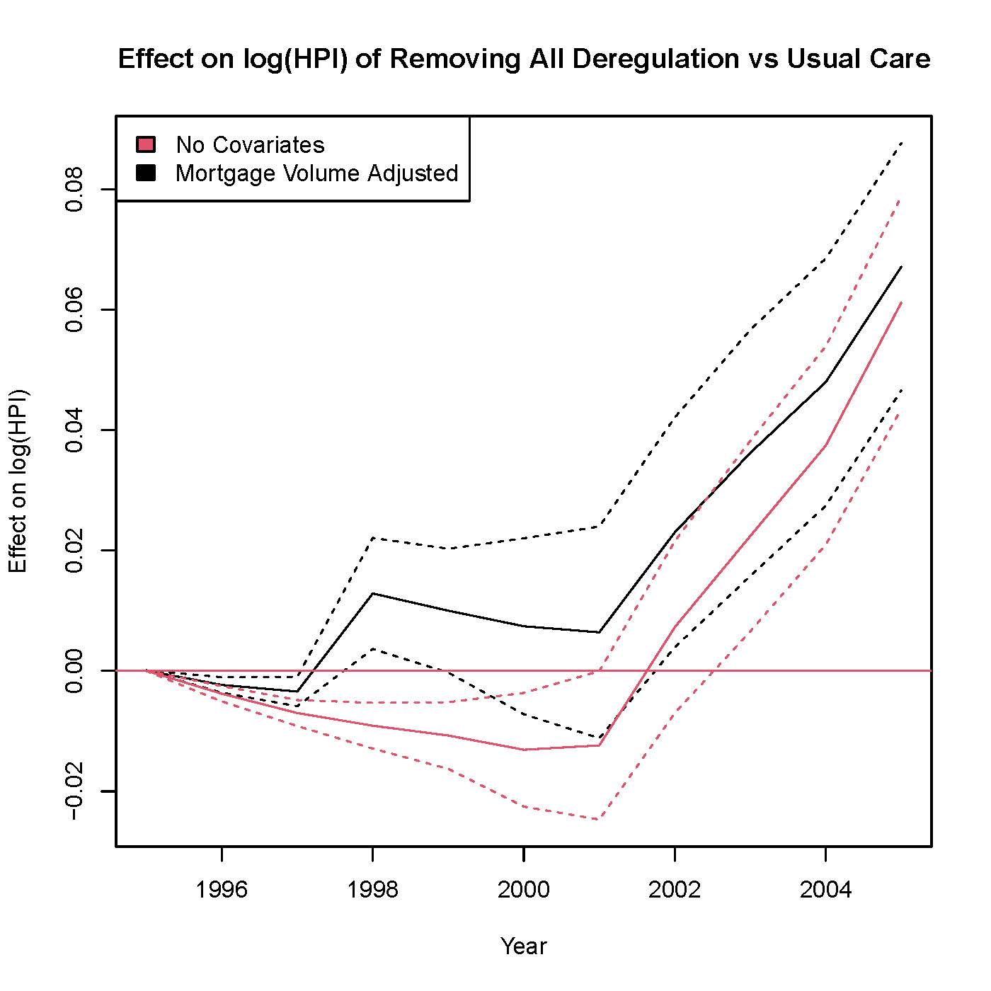
7.1 Impact of Bank Deregulation on Housing Prices

The Interstate Banking and Branching Efficiency Act, passed in 1994, allowed banks to operate across state borders without authorization from states. However, even after the bill was passed every state still imposed certain restrictions on interstate banking. Over time and in a staggered fashion, most states removed at least one of these restrictions. We estimate the effects of initial deregulation treated as a binary indicator variable on housing prices at the county level. Table 1 summarizes treatment timing over the period 1995-2005 considered in the study. To illustrate the benefits of our approach, we fit two coarse SNMMs–one with no time-varying covariates, and one that adjusts for and estimates effect heterogeneity as a function of mortgage volume in the previous year.

Year $\#$ Counties First Deregulating
1995 2
1996 246
1997 119
1998 416
2000 77
2001 55
Never 128
Table 1: Staggered deregulation by county

The no covariate coarse SNMM assumes that parallel trends holds unconditionally, i.e. $E[Y_{k}(\infty)-Y_{k-1}(\infty)|T=m]=[Y_{k}(\infty)-Y_{k-1}(\infty)|T=m]$ for all $m$ and $k$. We specified a nonparametric blip model $E[Y_{k}(m,1)-Y_{k}(\infty)|T=m]=\psi_{mk}^{c}$ with a separate parameter for each effect. We also specified nonparametric nuisance models for $E[A_{m}|T\geq m]$ and $E[H_{mk}^{c}(\psi^{c})-H_{mk-1}^{c}(\psi^{c})|T\geq m]$ with separate parameters for each $m$ and each $m,k$, respectively. We obtained point estimates using closed form linear estimators and estimated standard errors via bootstrap.

The coarse SNMM conditioning on mortgage volume from the previous year assumes $E[Y_{k}(\infty)-Y_{k-1}(\infty)|T=m,\bar{L}_{m}]=[Y_{k}(\infty)-Y_{k-1}(\infty)|T=m,\bar{L}_{m}]$ with $L_{m}$ denoting log mortgage volume in year $m-1$ and for all $m$ and $k$. Our blip model $E[Y_{k}(m,1)-Y_{k}(\infty)|T=m,\bar{L}_{m}]=\tau_{mk}+\beta L_{m}$ posited that the effect varies linearly with the previous year’s log mortgage volume. We specified nuisance models $E[A_{m}|T\geq m,\bar{L}_{m}]=\beta_{m0}+\beta_{m1}L_{m}+\beta_{m2}L_{m}^{2}$ and $E[H_{mk}^{c}(\psi^{c})-H_{mk-1}^{c}(\psi^{c})|T\geq m,\bar{L}_{m}]=\lambda_{mk0}+\lambda_{mk1}L_{m}$. We again obtained point estimates using closed form linear estimators and estimated standard errors via bootstrap.

Figure 1 displays the estimated effects on log housing price index of the deregulation that actually occurred compared to a counterfactual in which there was no deregulation (i.e. $E[Y_{k}-Y_{k}(\infty)]$ for each $k$). Estimated effects increase over time, which reflects some combination of effects of deregulation at a given location growing over time and increasing numbers of deregulated locations over time. Figure 2 displays for each lag $t$ the average effect over all deregulations $t$ years after the deregulation, i.e. $\frac{1}{\sum_{i=1}^{N}\sum_{m=1995}^{2005}\mathbbm{1}\{T_{i}=m\}}\sum_{i=1}^{N}\sum_{m=1995}^{2005}\mathbbm{1}\{T_{i}=m\}\hat{\gamma}^{c}_{m,m+t}(\bar{L}_{im})$. The quantity plotted in Figure 2 is also considered by Chaisemartin and D’Haultfoeuille (2021) and illustrates that on average a deregulation’s effects are estimated to grow over time. We do not directly compare our results with Chaisemartin and D’Haultfoeuille (2021) or Favara and Imbs (2015) because they each consider somewhat different estimands, but each of those analyses also found that deregulation increased housing prices and that effects grew over time.

In both Figures 1 and 2, the effect estimates from the coarse SNMM conditioning on mortgage volume are qualitatively similar but statistically significantly different from the effect estimates generated by the unconditional coarse SNMM, particularly at earlier years in Figure 1 and shorter time lags in Figure 1. At shorter time lags, the unconditional coarse SNMM estimates small negative effects of deregulation on housing prices, while the coarse SNMM conditional on mortgage volume estimates small positive effects. Perhaps the discrepancy arises because conditioning on mortgage volume corrects some bias.

We can also examine the estimate of the parameter $\beta$ from conditional coarse SNMM $E[Y_{k}(m,1)-Y_{k}(\infty)|T=m,\bar{L}_{m}]=\tau_{mk}+\beta L_{m}$ to learn about effect heterogeneity as a function of mortgage volume. We obtained the estimate $\hat{\beta}=0.044$ $(.95CI=[0.026,0.061])$, which is evidence that the effect of deregulation on housing prices is much greater in counties with higher mortgage volume. The interquartile range of log mortgage volume was 2.6, corresponding to a difference of 0.11 in estimated average effect of deregulation on housing prices between counties in the third and first quartiles of the mortgage volume distribution. This heterogeneity is quite strong relative to the scale of the average effects in Figures 1 and 2.

Refer to caption
Figure 1: Estimated effects on log housing price index of the deregulation that actually occurred compared to a counterfactual in which there was no deregulation, i.e. $E[Y_{k}-Y_{k}(\infty)]$ for each $k$
Refer to caption
Figure 2: For each lag $t$ the average effect over all deregulations $t$ years after the deregulation, i.e. $\frac{1}{\sum_{i=1}^{N}\sum_{m=1995}^{2005}\mathbbm{1}\{T_{i}=m\}}\sum_{i=1}^{N}\sum_{m=1995}^{2005}\mathbbm{1}\{T_{i}=m\}\hat{\gamma}^{c}_{m,m+t}(\bar{L}_{im})$.

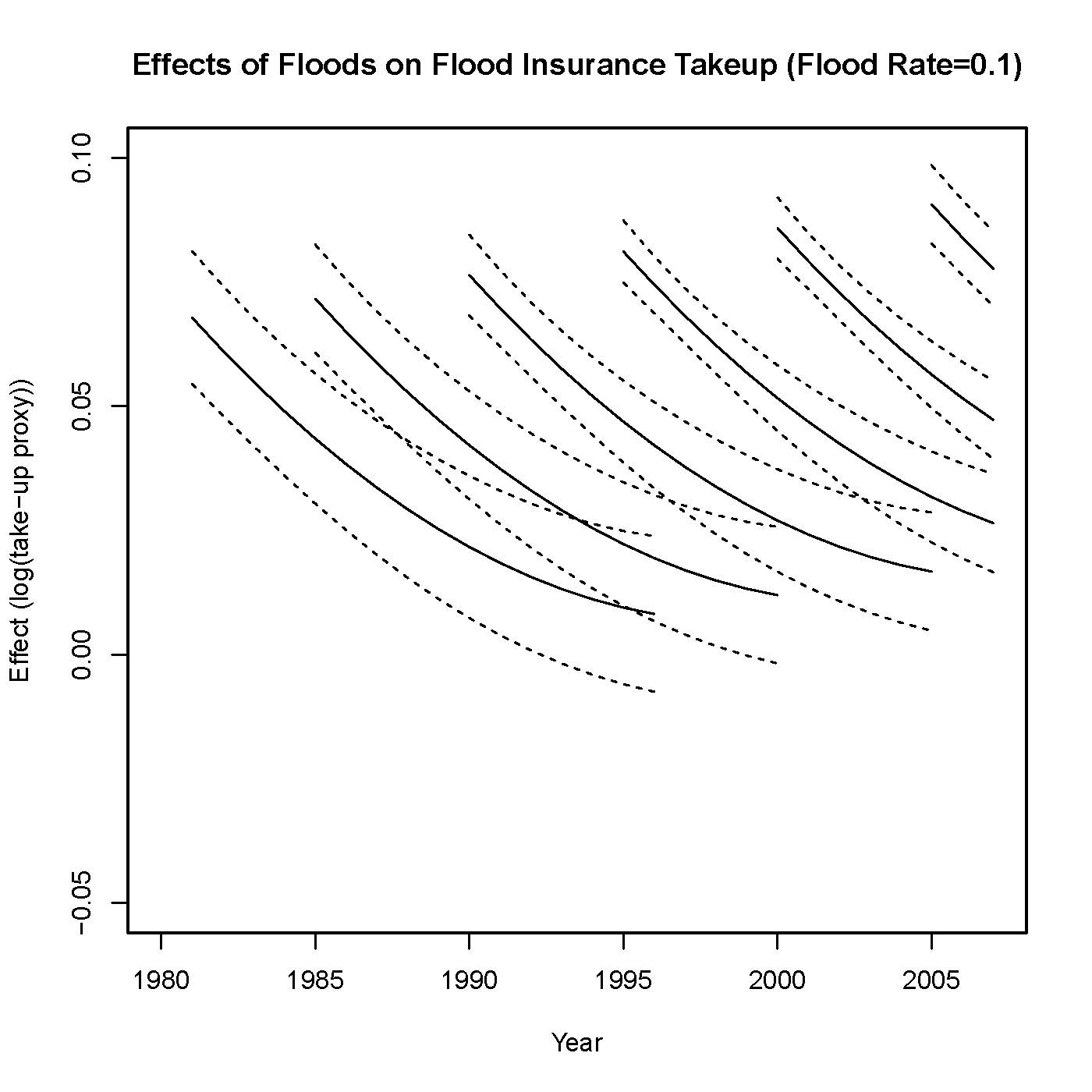
7.2 Impact of Floods on Flood Insurance

Gallagher (2014) used a fixed effects regression model to look at effects of floods on flood insurance coverage at the county level. He argued that each county?s flood risk is constant over time. We fit a standard SNMM under the assumption of parallel trends in insurance coverage absent future floods in counties with similar flood history from 1958. We specified a parametric linear blip model $\gamma_{mk}(\bar{l}_{m},\bar{a}_{m})=a_{m}(1,m-1980,k-m,(k-m)^{2},rate_{m-1})^{T}\psi$, where $rate_{m-1}$ denotes the county’s proportion of flood years since 1958. We specified nuisance models $E[A_{m}|\bar{A}_{m-1},\bar{L}_{m}]=\beta_{m0}+\beta_{m1}rate_{m-1}$ and $E[H_{mk}(\psi)-H_{mk-1}(\psi)|\bar{A}_{m-1},\bar{L}_{m}]=\lambda_{mk0}+\lambda_{mk1}rate_{m-1}$. We obtained blip model parameter estimates via closed form linear estimators and estimated standard errors via bootstrap. Each line in Figure 3 depicts the estimated effect on flood insurance uptake over 15 years of a flood at the leftmost time point on the line followed by no further floods over the 15 year period for a county with the median historical flood rate, i.e. $\gamma_{mk}(A_{m}=1,rate_{m-1}=rate_{median};\hat{\psi})$ for $k\in m,\ldots,m+15$. These quantities were directly extracted from our blip function estimates. We see that there is an initial surge in uptake followed by a steep decline, and the estimated initial surge is larger for more recent floods. We did not find statistically significant effect heterogeneity as a function of historical county flood rate. Gallagher (2014) obtained qualitatively similar results and argued that most of the decline in the effect of a flood is due to residents forgetting about it as opposed to migration. It might be interesting to explore other blip model specifications, perhaps conditioning on further aspects of flood history such as years since previous flood or on average flood insurance premiums in the area.

Refer to caption
Figure 3: Each line in Figure 3 depicts the estimated effect on flood insurance uptake over 15 years of a flood at the leftmost time point on the line followed by no further floods over the 15 year period for a county with the median historical flood rate, i.e. $\gamma_{mk}(A_{m}=1,rate_{m-1}=rate_{median};\hat{\psi})$ for $k\in m,\ldots,m+15$. These quantities were directly extracted from our blip function estimates.

8 Extensions

8.1 Efficiency Theory

In future work, we will also compute the efficient influence function and construct estimators that attain semiparametric efficiency bounds. It would further be interesting to compare the relative efficiency of our proposed estimators to those of Callaway and Sant’anna (2021) and Chaisemartin and D’Haultfoeuille (2020) for settings in which they target the same causal estimands under the same assumptions.

8.2 Sensitivity Analysis

Conditional parallel trends assumptions are strong and untestable, and sensitivity analysis for violations of the parallel trends assumption is therefore desirable. We adapt the approach to sensitivity analysis for unobserved confounding in SNMMs of Robins et al (2000) and Yang and Lok (2018) to sensitivity analysis for non-parallel trends. We describe a general class of bias functions characterizing deviations from parallel trends given covariate history. For any particular bias function from this class, we provide a corresponding unbiased estimate of (coarse) SNMM parameters assuming that the bias function is correctly specified. An analyst can then execute a sensitivity analysis by specifying a plausible range of bias functions (e.g. a grid of parameters covering a plausible range within a parametric subclass of bias functions) and producing the corresponding range of plausible effect estimates. This approach to sensitivity analysis is complementary to that developed by Rambachan and Roth (2022), as it allows deviations to depend on covariates and allows for sensitivity analysis of all SNMM parameters (e.g. those characterizing effect heterogeneity) and derived quantities. In the exposition below, we focus for simplicity on coarse SNMMs with binary treatments, but extensions to the general case are straightforward.

Define

$\displaystyle\begin{split}&c(\bar{l}_{m},k)=\\ &E[Y_{k}(\infty)-Y_{k-1}(\infty)|\bar{L}_{m},T\geq m,A_{m}=1]-E[Y_{k}(\infty)-Y_{k-1}(\infty)|\bar{L}_{m},T\geq m,A_{m}=0].\end{split}$ (38)

$c(\bar{l}_{m},k)$ characterizes the magnitude of deviation from the parallel trends assumption (LABEL:coarse_parallel). It is a general function in that it allows deviations to depend both on covariate history and time horizon $k$.

Given a bias function (LABEL:bias_function), define the bias adjusted version of the ‘blipped down’ quantity (12) as

$$H_{mk}^{c,a}(\gamma^{c})\equiv H_{mk}^{c}(\gamma^{c})-\sum_{j=m}^{k}Pr(1-A_{j}|\bar{L}_{j},T\geq j)(2A_{j}-1)c(\bar{L}_{j},k)\mathbbm{1}\{T\geq j\},$$ (39)

where $H_{mk}^{c}$ is defined in (12).

Lemma 1.

If (LABEL:bias_function) is correctly specified, then

$\displaystyle\begin{split}&E[H_{mk}^{c,a}(\gamma^{c*})-H_{mk-1}^{c}(\gamma^{c*})|\bar{L}_{m},T\geq m,A_{m}]\\ &=E[H_{mk}^{c,a}(\gamma^{c*})-H_{mk-1}^{c}(\gamma^{c*})|\bar{L}_{m},T\geq m].\end{split}$ (40)
Proof.

See Appendix D. ∎

Lemma 1 states that under correct specification of the bias function (LABEL:bias_function), the conditional expectation of $H_{mk}^{c,a}(\gamma^{c*})-H_{mk-1}^{c}(\gamma^{c*})$ does not depend on $A_{m}$. This is the same crucial property satisfied by $H_{mk}^{c}(\gamma^{c*})-H_{mk-1}^{c}(\gamma^{c*})$ in (LABEL:coarse_id) that enabled identification of $\gamma^{c*}$. Thus, it follows that identification and estimation of $\gamma^{c*}$ under bias function (LABEL:bias_function) may proceed exactly as identification and estimation of $\gamma^{c*}$ under the parallel trends assumption (LABEL:coarse_parallel) except substituting $H_{mk}^{c,a}(\gamma^{c})-H_{mk-1}^{c}(\gamma^{c*})$ for $H_{mk}^{c}(\gamma^{c})-H_{mk-1}^{c}(\gamma^{c*})$. In future work, we will flesh out this sensitivity analysis framework and explore suitable parameterizations of the bias function for tractable and informative sensitivity analysis.

8.3 Survival Outcomes

Piccioto et al. (2012) introduced Structural Nested Cumulative Failure Time Models (SNCFTMs) for time to event outcomes. We can also identify the parameters of these models under a delayed parallel survival curves assumption and a delayed treatment effect assumption. The delayed parallel survival curves assumption states that treated and untreated subjects at time $m$ who have similar observed histories through time $m$ have parallel counterfactual untreated survival probability curves after time $m+\tau$ for some duration $\tau$. The delayed treatment effect assumption states that treatment given at time $m$ has no effect on outcomes until at least $m+\tau$. Delayed treatment effects occur frequently, for example many vaccines have delayed effects and exposures to toxic chemicals often take a long time to lead to cancer diagnosis. Delayed parallel survival curves imply that the impact of unobserved confounders on survival probabilities on a multiplicative scale vanishes in less than $\tau$ time steps. This strange combination of assumptions (i.e. that treatments must have delayed effects but unobserved confounders only short term effects) leads us not to present our current results for survival outcomes, but we do wish to point out that extension of DiD to time-to-event settings via structural nested models may still be a promising direction for future work.

8.4 Controlled Direct Effects

We mentioned in passing that SNMM treatments may be multi-dimensional. In particular, we wish to emphasize that this enables estimation of controlled direct effects (CDEs) (Robins and Greenland, 1992). Such effects might be of interest either to make the parallel trends assumption more plausible or to explore mechanisms. For an example of strengthening the parallel trends assumption through controlled direct effects, suppose an investigator is interested in effects of Medicaid expansion on some outcome that is impacted both by Medicaid and the minimum wage. Given that states that expand Medicaid in a given year are also more likely to later increase the minimum wage, future minimum wage increases can lead to violations of the parallel trends assumption in an analysis where Medicaid is the sole treatment. However, by estimating the joint effect of Medicaid expansion and no future minimum wage expansion (i.e. the controlled direct effect of Medicaid expansion setting minimum wage increases to 0), that particular threat to the parallel trends assumption is eliminated. See Robins and Greenland (1992) for discussion of controlled direct effects for exploring mechanisms. See Blackwell et al (2022) for an alternative approach to estimating CDEs under parallel trends assumptions in a somewhat different setting.

For a two dimensional treatment $(\bar{A},\bar{R})$, consider the effects

$\displaystyle\begin{split}&\gamma_{mk}^{CDE*}((\bar{a}_{m},\bar{r}_{m}),\bar{l}_{m})=\\ &E[Y_{k}(\bar{a}=(\bar{A}_{m},\underline{0}),\bar{r}=(\bar{R}_{m},\underline{0}))-Y_{k}(\bar{a}=(\bar{A}_{m-1},\underline{0}),\bar{r}=(\bar{R}_{m-1},\underline{0}))|\bar{A}_{m}=\bar{a}_{m},\bar{R}_{m}=\bar{r}_{m},\bar{L}_{m}=\bar{l}_{m}].\end{split}$ (41)

These are just the blip functions of a standard SNMM with a two dimensional treatment, and are therefore identified and can be consistently and asymptotically normally estimated by the results of Section 4. Then the quantity $\gamma_{mk}^{CDE*}((\bar{a}_{m},\bar{r}_{m}),\bar{l}_{m})$ with $r_{m}=0$ might be of particular interest as the controlled direct effect of a treatment $a_{m}$ at time $m$ setting $\underline{R}_{m}$ to 0 in subjects with $R_{m}=0$ and $\bar{L}_{m}=\bar{l}_{m}$. Revisiting the flood example, suppose that $\bar{A}$ denotes flood history and $\bar{R}$ denotes wildfire history. Suppose floods are associated with future wild fires, which is a threat to the validity of the parallel trends assumption in an analysis of floods alone, but interest still centers on the impact of floods. Or, alternatively, suppose that floods make future wildfires less likely by clearing brush or dampening the ground (a possibility that might only be plausible to those as ignorant of this topic as the authors), and interest centers on the psychological impact of floods on insurance take-up as opposed to the influence through occurrence of other natural disasters. In either of the above two scenarios, the quantities $\gamma_{mk}^{CDE*}((\bar{a}_{m},\bar{r}_{m}),\bar{l}_{m})$ with $r_{m}=0$ (perhaps marginalized over $\bar{L}_{m}$) yielding the controlled direct effects of floods in the absence of future fires would be of interest.

Now, consider the controlled direct effects of a two dimensional coarse intervention

$$E[Y_{k}(T_{A}=m,A_{m}=a_{m},T_{R}=\infty)-Y_{k}(T_{A}=T_{R}=\infty)|T_{A}=m,A_{m}=a_{m},T_{R}>m,\bar{L}_{m}],$$ (42)

where $T_{A}$ denotes the first time of departure of treatment $A$ from its baseline level 0 and $T_{R}$ denotes the first time of departure of treatment $R$ from its baseline level 0. These are the effects of departing from the $A$ baseline treatment level for the first time at time $m$ and never departing from the $R$ baseline treatment level compared to never departing from either the $A$ or $R$ baseline levels in those who did depart from baseline $A$ treatment at time $m$ and had not yet departed from the baseline $R$ treatment. We have seen how to identify and estimate the second term in the difference (42), i.e. $E[Y_{k}(T_{A}=T_{R}=\infty)|T_{A}=m,A_{m}=a_{m},T_{R}>m,\bar{L}_{m}]$, via a coarse SNMM for two dimensional treatment $\bar{A},\bar{R}$ in Section 3. To identify and estimate the first term $E[Y_{k}(T_{A}=m,A_{m}=a_{m},T_{R}=\infty)|T_{A}=m,A_{m}=a_{m},T_{R}>m,\bar{L}_{m}]$, we can specify a separate coarse SNMM for effects of $R$. In particular, we can make the parallel trends assumption

$\displaystyle\begin{split}&E[Y_{k}(T_{A}=m,A_{m}=a_{m},T_{R}=\infty)-Y_{k-1}(T_{A}=m,A_{m}=a_{m},T_{R}=\infty)|T_{A}=m,A_{m},T_{R}\geq j,R_{j},\bar{L}_{j}]=\\ &E[Y_{k}(T_{A}=m,A_{m}=a_{m},T_{R}=\infty)-Y_{k-1}(T_{A}=m,A_{m}=a_{m},T_{R}=\infty)|T_{A}=m,A_{m},T_{R}>j,\bar{L}_{j}]\\ &\text{for all k>j $\geq$ m}\end{split}$ (43)

for treatment $R$ in the subpopulation starting treatment $A$ at $m$. Then, by the results of Section 3, the coarse SNMM for the effects of $R$ in the cohort of subjects with $T_{A}=m$, i.e.

$\displaystyle\begin{split}&\gamma^{R,c}_{mjk}(\bar{l}_{j},r_{j},a_{m})=\\ &E[Y_{k}(T_{A}=m,a_{m},T_{R}=j,r_{j})-Y_{k}(T_{A}=m,a_{m},T_{R}=\infty)|T_{A}=m,T_{R}=j,R_{j}=r_{j},\bar{L}_{j}]\end{split}$ (44)

is identified. We can then consistently estimate $E[Y_{k}(T_{A}=m,A_{m}=a_{m},T_{R}=\infty)|T_{A}=m,A_{m}=a_{m},T_{R}>m,\bar{L}_{m}]$ by $\mathbbm{P}^{T_{A}=m,T_{R}>m}[H_{mk}^{R,c}(\hat{\gamma}^{R,c})]$, where

$$H_{mk}^{R,c}(\gamma^{R,c})\equiv Y_{k}-\sum_{j=m}^{k-1}\mathbbm{1}\{T_{R}=j\}\gamma^{R,c}_{mjk}(\bar{L}_{j},R_{j},a_{m}).$$ (45)

Thus, we can consistently estimate both terms in the difference (42) defining the CDE.

8.5 Repeated Cross Sectional Data

In this paper, we have assumed throughout that panel data are available. However, many DiD applications use repeated cross sectional data with different participants in each cross section. It will be interesting to see how our approach and assumptions might be modified to accommodate repeated cross sectional data.

9 Conclusion

To summarize, we have shown that structural nested mean models expand the set of causal questions that can be addressed under parallel trends assumptions. In particular, we have shown that coarse additive SNMMs, standard additive SNMMs, and multiplicative coarse or standard SNMMs can all be identified under time-varying conditional parallel trends assumptions. Using these models, we can do many things that were not previously possible in DiD studies, such as: characterize effect heterogeneity as a function of time-varying covariates (e.g. mortgage volume in the bank deregulation analysis), identify the effect of one final blip of treatment (as in the flood analysis) and other derived contrasts, and adjust for time-varying trend confounders (again, illustrated by mortgage volume analysis). Under stronger assumptions limiting effect heterogeneity, we have also explained how to estimate counterfactual expectations under general regimes and optimal treatment regimes via optimal regime SNMMs. We hope these new capabilities can be put to use in a wide variety of applications.

10 Bibliography

Athey, Susan, and Guido W. Imbens. "Identification and inference in nonlinear difference-in-differences models." Econometrica 74, no. 2 (2006): 431-497.

Athey, Susan, and Guido W. Imbens. Design-based analysis in difference-in-differences settings with staggered adoption. No. w24963. National Bureau of Economic Research, 2018.

Bojinov, Iavor, Ashesh Rambachan, and Neil Shephard. "Panel experiments and dynamic causal effects: A finite population perspective." Quantitative Economics 12, no. 4 (2021): 1171-1196.

Callaway, Brantly, and Pedro HC Sant?Anna. "Difference-in-differences with multiple time periods." Journal of Econometrics 225, no. 2 (2021): 200-230.

Card, D. and Krueger, A. B. (1993). Minimum wages and employment: A case study of the fast food industry in New Jersey and Pennsylvania. Tech. rep., National Bureau of Economic Research.

De Chaisemartin, Clement, and Xavier D’Haultfoeuille. "Difference-in-differences estimators of intertemporal treatment effects." Available at SSRN 3731856 (2020).

Chernozhukov, Victor, Denis Chetverikov, Mert Demirer, Esther Duflo, Christian Hansen, Whitney Newey, and James Robins. "Double/debiased machine learning for treatment and structural parameters." (2018): C1-C68.

Lok, Judith J., and Victor DeGruttola. "Impact of time to start treatment following infection with application to initiating HAART in HIV?positive patients." Biometrics 68, no. 3 (2012): 745-754.

Picciotto, Sally, et al. "Structural nested cumulative failure time models to estimate the effects of interventions." Journal of the American Statistical Association 107.499 (2012): 886-900.

Rambachan, Ashesh, and Jonathan Roth. A More Credible Approach to Parallel Trends. Working Paper, 2022.

Robins, James M. "Correcting for non-compliance in randomized trials using structural nested mean models." Communications in Statistics-Theory and methods 23.8 (1994): 2379-2412.

Robins J.M., 1997, Causal inference from complex longitudinal data, In: Latent Variable Modeling and Applications to Causality, Lecture Notes in Statistics (120), M. Berkane, Editor. NY: Springer Verlag, 69-117.

Robins, James M. "Correction for noncompliance in equivalence trials." Statistics in medicine 17, no. 3 (1998): 269-302.

Robins, James M. "Marginal structural models versus structural nested models as tools for causal inference." In Statistical models in epidemiology, the environment, and clinical trials, pp. 95-133. Springer, New York, NY, 2000.

Robins, James M. "Optimal structural nested models for optimal sequential decisions." In Proceedings of the second seattle Symposium in Biostatistics, pp. 189-326. Springer, New York, NY, 2004.

Robins, James M., and Sander Greenland. "Identifiability and exchangeability for direct and indirect effects." Epidemiology (1992): 143-155.

Robins, James M., Andrea Rotnitzky, and Daniel O. Scharfstein. "Sensitivity analysis for selection bias and unmeasured confounding in missing data and causal inference models." In Statistical models in epidemiology, the environment, and clinical trials, pp. 1-94. Springer, New York, NY, 2000.

Roth, Jonathan, Pedro HC Sant’Anna, Alyssa Bilinski, and John Poe. "What’s Trending in Difference-in-Differences? A Synthesis of the Recent Econometrics Literature." arXiv preprint arXiv:2201.01194 (2022).

Smucler, Ezequiel, Andrea Rotnitzky, and James M. Robins. "A unifying approach for doubly-robust $\ell_{1}$ regularized estimation of causal contrasts." arXiv preprint arXiv:1904.03737 (2019).

Snow, J. (1855). On the mode of communication of Cholera. John Churchill.

Stuart, E. A., Huskamp, H. A., Duckworth, K., Simmons, J., Song, Z., Chernew, M. E., and Barry, C. L. (2014). Using propensity scores in difference-in-differences models to estimate the effects of a policy change. Health Services and Outcomes Research Methodology, 14(4), 166-182.

Sofer, Tamar, David B. Richardson, Elena Colicino, Joel Schwartz, and Eric J. Tchetgen Tchetgen. "On negative outcome control of unobserved confounding as a generalization of difference-in-differences." Statistical science: a review journal of the Institute of Mathematical Statistics 31, no. 3 (2016): 348.

Van der Vaart, Aad W. Asymptotic statistics. Vol. 3. Cambridge university press, 2000.

Vansteelandt, Stijn, and Marshall Joffe. "Structural nested models and G-estimation: the partially realized promise." Statistical Science 29, no. 4 (2014): 707-731.

Yang, Shu, and Judith J. Lok. "Sensitivity analysis for unmeasured confounding in coarse structural nested mean models." Statistica Sinica 28, no. 4 (2018): 1703.

Zeldow, Bret, and Laura A. Hatfield. "Confounding and Regression Adjustment in Difference-in-Differences." arXiv preprint arXiv:1911.12185 (2019).

Appendix

Appendix A: Proof of Theorem 1

Part(i)

E[Umkc(sm,γc)]=E[E[Umkc(sm,γc)|L¯m,A¯m]]=E[𝟙{Tm}E[Hm,kc(γc)Hm,k1c(γc)|L¯m,A¯m1](sm(k,L¯m,A¯m)E[sm(k,L¯m,A¯m)|L¯m,A¯m1])]by (LABEL:coarse_id)=E[𝟙{Tm}E[Hm,kc(γc)Hm,k1c(γc)|L¯m,A¯m1]×E[sm(k,L¯m,A¯m)E[sm(k,L¯m,A¯m)|L¯m,A¯m1]|A¯m1,L¯m]]by nested expectations=0𝐸delimited-[]subscriptsuperscript𝑈𝑐𝑚𝑘subscript𝑠𝑚superscript𝛾𝑐𝐸delimited-[]𝐸delimited-[]conditionalsubscriptsuperscript𝑈𝑐𝑚𝑘subscript𝑠𝑚superscript𝛾𝑐subscript¯𝐿𝑚subscript¯𝐴𝑚𝐸delimited-[]1𝑇𝑚𝐸delimited-[]subscriptsuperscript𝐻𝑐𝑚𝑘superscript𝛾𝑐conditionalsubscriptsuperscript𝐻𝑐𝑚𝑘1superscript𝛾𝑐subscript¯𝐿𝑚subscript¯𝐴𝑚1subscript𝑠𝑚𝑘subscript¯𝐿𝑚subscript¯𝐴𝑚𝐸delimited-[]conditionalsubscript𝑠𝑚𝑘subscript¯𝐿𝑚subscript¯𝐴𝑚subscript¯𝐿𝑚subscript¯𝐴𝑚1by (LABEL:coarse_id)𝐸delimited-[]1𝑇𝑚𝐸delimited-[]subscriptsuperscript𝐻𝑐𝑚𝑘superscript𝛾𝑐|subscriptsuperscript𝐻𝑐𝑚𝑘1superscript𝛾𝑐subscript¯𝐿𝑚subscript¯𝐴𝑚1𝐸delimited-[]subscript𝑠𝑚𝑘subscript¯𝐿𝑚subscript¯𝐴𝑚conditional𝐸delimited-[]conditionalsubscript𝑠𝑚𝑘subscript¯𝐿𝑚subscript¯𝐴𝑚subscript¯𝐿𝑚subscript¯𝐴𝑚1subscript¯𝐴𝑚1subscript¯𝐿𝑚by nested expectations0\displaystyle\begin{split}&E[U^{c}_{mk}(s_{m},\gamma^{c*})]=E[E[U^{c}_{mk}(s_{m},\gamma^{c*})|\bar{L}_{m},\bar{A}_{m}]]\\ &=E[\\ &\mathbbm{1}\{T\geq m\}E[H^{c}_{m,k}(\gamma^{c*})-H^{c}_{m,k-1}(\gamma^{c*})|\bar{L}_{m},\bar{A}_{m-1}](s_{m}(k,\overline{L}_{m},\overline{A}_{m})-E[s_{m}(k,\overline{L}_{m},\overline{A}_{m})|\bar{L}_{m},\bar{A}_{m-1}])\\ &]\\ &\text{by (\ref{coarse_id})}\\ &=E[\\ &\mathbbm{1}\{T\geq m\}E[H^{c}_{m,k}(\gamma^{c*})-H^{c}_{m,k-1}(\gamma^{c*})|\bar{L}_{m},\bar{A}_{m-1}]\times\\ &E[s_{m}(k,\overline{L}_{m},\overline{A}_{m})-E[s_{m}(k,\overline{L}_{m},\overline{A}_{m})|\bar{L}_{m},\bar{A}_{m-1}]|\bar{A}_{m-1},\bar{L}_{m}]\\ &]\\ &\text{by nested expectations}\\ &=0\end{split} (46)

The above establishes that the true blip functions are a solution to these equations. The proof of uniqueness follows from the two Lemmas below.

Lemma 2.

Any functions $\gamma^{c}$ satisfying (15) for all $s_{m}(k,\bar{l}_{m},\bar{a}_{m})$ also satisfies (20), i.e.

$$E[H_{mk}(\gamma)-H_{mk-1}(\gamma)|\bar{A}_{m}=\bar{a}_{m},\bar{L}_{m}]=E[H_{mk}(\gamma)-H_{mk-1}(\gamma)|\bar{A}_{m}=(\bar{a}_{m-1},0),\bar{L}_{m}]\forall k>m.$$
Proof.

Since (15) must hold for all $s_{m}(k,\bar{l}_{m},\bar{a}_{m})$, in particular it must hold for

$$s_{m}(k,\bar{l}_{m},\bar{a}_{m})=E[H^{c}_{mk}(\gamma^{c})-H^{c}_{mk-1}(\gamma^{c})|\bar{A}_{m},\bar{L}_{m}].$$

Plugging this choice of $s_{m}(k,\bar{l}_{m},\bar{a}_{m})$ into $U^{c}_{mk}$, we get

$\displaystyle E[\{H^{c}_{mk}(\gamma^{c})-H^{c}_{mk-1}(\gamma^{c})\}\times$
$\displaystyle\{E[H^{c}_{mk}(\gamma^{c})-H^{c}_{mk-1}(\gamma^{c})|\bar{A}_{m},\bar{L}_{m}]-E[H^{c}_{mk}(\gamma^{c})-H^{c}_{mk-1}(\gamma^{c})|\bar{L}_{m},\bar{A}_{m-1}]\}]=0$
$\displaystyle\implies$
$\displaystyle E[H^{c}_{mk}(\gamma^{c})-H^{c}_{mk-1}(\gamma^{c})|\bar{A}_{m},\bar{L}_{m}]=E[H^{c}_{mk}(\gamma^{c})-H^{c}_{mk-1}(\gamma^{c})|\bar{L}_{m},\bar{A}_{m-1}],$

which proves the result. ∎

Lemma 3.

$\gamma^{c*}$ are the unique functions satisfying (LABEL:coarse_id)

Proof.

We proceed by induction. Suppose for any $k$ there exist other functions $\gamma^{c^{\prime}}$ in addition to $\gamma^{c*}$ satisfying (LABEL:coarse_id), i.e.

$\displaystyle E[H^{c}_{(k-1)k}(\gamma^{c*})-H^{c}_{(k-1)(k-1)}(\gamma^{c*})|(\bar{A}_{k-2}=0,A_{k-1}),\bar{L}_{k-1}]=$
$\displaystyle E[H^{c}_{(k-1)k}(\gamma^{c*})-H^{c}_{(k-1)(k-1)}(\gamma^{c*})|(\bar{A}_{k-2}=0,0),\bar{L}_{k-1}]$
$\displaystyle and$
$\displaystyle E[H^{c}_{(k-1)k}(\gamma^{c^{\prime}})-H^{c}_{(k-1)(k-1)}(\gamma^{c^{\prime}})|(\bar{A}_{k-2}=0,0),\bar{L}_{k-1}]=$
$\displaystyle E[H^{c}_{(k-1)k}(\gamma^{{}^{\prime}})-H^{c}_{(k-1)(k-1)}(\gamma^{c^{\prime}})|(\bar{A}_{k-2}=0,0),\bar{L}_{k-1}].$

Differencing both sides of the above equations using the definition of $H^{c}_{mk}(\gamma^{c})$ yields that

$\displaystyle E[\gamma^{c*}_{(k-1)k}(\bar{L}_{k-1})\mathbbm{1}\{T=k-1\}-\gamma^{c^{\prime}}_{(k-1)k}(\bar{L}_{k-1})\mathbbm{1}\{T=k-1\}|(\bar{A}_{k-2}=0,A_{k-1}),\bar{L}_{k-1}]$
$\displaystyle=\gamma^{c*}_{(k-1)k}(\bar{L}_{k-1})\mathbbm{1}\{T=k-1\}-\gamma^{c^{\prime}}_{(k-1)k}(\bar{L}_{k-1})\mathbbm{1}\{T=k-1\}$
$\displaystyle=E[\gamma^{c*}_{(k-1)k}(\bar{L}_{k-1})\mathbbm{1}\{T=k-1\}-\gamma^{c^{\prime}}_{(k-1)k}(\bar{L}_{k-1})\mathbbm{1}\{T=k-1\}|(\bar{A}_{k-2}=0,0),\bar{L}_{k-1}]$
$\displaystyle=0.$

This establishes that $\gamma^{c*}_{(k-1)k}=\gamma^{c^{\prime}}_{(k-1)k}$ for all $k$. Suppose for the purposes of induction that we have established that $\gamma^{c*}_{(k-j)k}=\gamma^{c^{\prime}}_{(k-j)k}$ for all $k$ and all $j\in\{1,\ldots,n\}$. Now consider $\gamma^{c*}_{(k-(n+1))k}$ and $\gamma^{c^{\prime}}_{(k-(n+1))k}$. Again we have that

$\displaystyle E[H^{c}_{(k-(n+1))k}(\gamma^{c*})-H^{c}_{(k-(n+1))(k-1)}(\gamma^{c*})|(\bar{A}_{k-(n+2)}=0,A_{k-(n+1)}),\bar{L}_{k-(n+1)}]=$
$\displaystyle E[H^{c}_{(k-(n+1))k}(\gamma^{c*})-H^{c}_{(k-(n+1))(k-1)}(\gamma^{c*})|(\bar{A}_{k-(n+2)}=0,0),\bar{L}_{k-(n+1)}]$
$\displaystyle and$
$\displaystyle E[H^{c}_{(k-(n+1))k}(\gamma^{c^{\prime}})-H^{c}_{(k-(n+1))(k-1)}(\gamma^{c^{\prime}})|(\bar{A}_{k-(n+2)}=0,A_{k-(n+1)}),\bar{L}_{k-(n+1)}]=$
$\displaystyle E[H^{c}_{(k-(n+1))k}(\gamma^{c^{\prime}})-H^{c}_{(k-(n+1))(k-1)}(\gamma^{c^{\prime}})|(\bar{A}_{k-(n+2)}=0,0),\bar{L}_{k-(n+1)}].$

And again we can difference both sides of these equations plugging in the expanded definition of $H^{c}_{(k-(n+1))k}(\gamma^{c})$ to obtain

$\displaystyle\begin{split}&E[\{Y_{k}-\sum_{j=k-(n+1)}^{k-1}\gamma^{c*}_{jk}(\bar{L}_{j})\mathbbm{1}\{T=j\}\}-\\ &\{Y_{k}-\sum_{j=k-(n+1)}^{k-1}\gamma^{c^{\prime}}_{jk}(\bar{L}_{j})\mathbbm{1}\{T=j\}\}|(\bar{A}_{k-(n+2)}=0,A_{k-(n+1)}),\bar{L}_{k-(n+1)}]\\ &=E[\{Y_{k}-\sum_{j=k-(n+1)}^{k-1}\gamma^{c*}_{jk}(\bar{L}_{j})\mathbbm{1}\{T=j\}\}-\\ &\{Y_{k}-\sum_{j=k-(n+1)}^{k-1}\gamma^{c^{\prime}}_{jk}(\bar{L}_{j})\mathbbm{1}\{T=j\}\}|(\bar{A}_{k-(n+2)},0),\bar{L}_{k-(n+1)}].\end{split}$ (47)

Under our inductive assumption, (LABEL:lemma2_step1_coarse) reduces to

$\displaystyle E[\gamma^{c*}_{(k-(n+1))k}(\bar{L}_{k-(n+1)})\mathbbm{1}\{T=k-(n+1)\}-$
$\displaystyle\gamma^{c^{\prime}}_{(k-(n+1))k}(\bar{L}_{k-(n+1)})\mathbbm{1}\{T=k-(n+1)\}|(\bar{A}_{k-(n+2)}=0,A_{k-(n+1)}),\bar{L}_{k-(n+1)}]$
$\displaystyle=\gamma^{c*}_{(k-(n+1))k}(\bar{L}_{k-(n+1)})\mathbbm{1}\{T=k-(n+1)\}-\gamma^{c^{\prime}}_{(k-(n+1))k}(\bar{L}_{k-(n+1)})\mathbbm{1}\{T=k-(n+1)\}$
$\displaystyle=E[\gamma^{c*}_{(k-(n+1))k}(\bar{L}_{k-(n+1)})\mathbbm{1}\{T=k-(n+1)\}-$
$\displaystyle\gamma^{c^{\prime}}_{(k-(n+1))k}(\bar{L}_{k-1})\mathbbm{1}\{T=k-(n+1)\}|(\bar{A}_{k-(n+2)}=0,0),\bar{L}_{k-(n+1)}]$
$\displaystyle=0,$

proving that $\gamma_{(k-(n+1))k}^{c*}=\gamma_{(k-(n+1))k}^{c^{\prime}}$ for all $k$. Hence, by induction, the result follows. ∎

Uniqueness is a direct corollary of Lemmas 2 and 3.

Part (ii)

E[Umkc(sm,γ¯mc,v~mc,E~Am|L¯m,A¯m1)]=E[E[Umkc(sm,γ¯mc,v~mc,E~Am|L¯m,A¯m1)|L¯m,A¯m]]=E[E[Hm,kc(γc)Hm,k1c(γc)v~mc(k,L¯m,A¯m1,γc)|L¯m,A¯m1]q(L¯m,A¯m1)×(sm(k,L¯m,A¯m)E~Am|L¯m,A¯m1[sm(k,L¯m,A¯m)|L¯m,A¯m1])]by (LABEL:coarse_id)=E[E[E[Hm,kc(γc)Hm,k1c(γc)v~mc(k,L¯m,A¯m1,γc)|L¯m,A¯m1]q(L¯m,A¯m1)×E[sm(k,L¯m,A¯m)E~Am|L¯m,A¯m1[sm(k,L¯m,A¯m)|L¯m,A¯m1]|L¯m,A¯m1]]]𝐸delimited-[]subscriptsuperscript𝑈𝑐𝑚𝑘subscript𝑠𝑚superscriptsubscript¯𝛾𝑚𝑐superscriptsubscript~𝑣𝑚𝑐subscript~𝐸conditionalsubscript𝐴𝑚subscript¯𝐿𝑚subscript¯𝐴𝑚1𝐸delimited-[]𝐸delimited-[]conditionalsubscriptsuperscript𝑈𝑐𝑚𝑘subscript𝑠𝑚superscriptsubscript¯𝛾𝑚𝑐superscriptsubscript~𝑣𝑚𝑐subscript~𝐸conditionalsubscript𝐴𝑚subscript¯𝐿𝑚subscript¯𝐴𝑚1subscript¯𝐿𝑚subscript¯𝐴𝑚𝐸delimited-[]𝐸delimited-[]subscriptsuperscript𝐻𝑐𝑚𝑘superscript𝛾𝑐subscriptsuperscript𝐻𝑐𝑚𝑘1superscript𝛾𝑐|superscriptsubscript~𝑣𝑚𝑐𝑘subscript¯𝐿𝑚subscript¯𝐴𝑚1superscript𝛾𝑐subscript¯𝐿𝑚subscript¯𝐴𝑚1𝑞subscript¯𝐿𝑚subscript¯𝐴𝑚1subscript𝑠𝑚𝑘subscript¯𝐿𝑚subscript¯𝐴𝑚subscript~𝐸conditionalsubscript𝐴𝑚subscript¯𝐿𝑚subscript¯𝐴𝑚1delimited-[]conditionalsubscript𝑠𝑚𝑘subscript¯𝐿𝑚subscript¯𝐴𝑚subscript¯𝐿𝑚subscript¯𝐴𝑚1by (LABEL:coarse_id)𝐸delimited-[]𝐸delimited-[]𝐸delimited-[]subscriptsuperscript𝐻𝑐𝑚𝑘superscript𝛾𝑐subscriptsuperscript𝐻𝑐𝑚𝑘1superscript𝛾𝑐|superscriptsubscript~𝑣𝑚𝑐𝑘subscript¯𝐿𝑚subscript¯𝐴𝑚1superscript𝛾𝑐subscript¯𝐿𝑚subscript¯𝐴𝑚1𝑞subscript¯𝐿𝑚subscript¯𝐴𝑚1𝐸delimited-[]subscript𝑠𝑚𝑘subscript¯𝐿𝑚subscript¯𝐴𝑚|subscript~𝐸conditionalsubscript𝐴𝑚subscript¯𝐿𝑚subscript¯𝐴𝑚1delimited-[]|subscript𝑠𝑚𝑘subscript¯𝐿𝑚subscript¯𝐴𝑚subscript¯𝐿𝑚subscript¯𝐴𝑚1subscript¯𝐿𝑚subscript¯𝐴𝑚1\displaystyle\begin{split}&E[U^{c\dagger}_{mk}(s_{m},\underline{\mathbf{\gamma}}_{m}^{c*},\widetilde{v}_{m}^{c},\widetilde{E}_{A_{m}|\overline{L}_{m},\overline{A}_{m-1}})]=E[E[U^{c\dagger}_{mk}(s_{m},\underline{\mathbf{\gamma}}_{m}^{c*},\widetilde{v}_{m}^{c},\widetilde{E}_{A_{m}|\overline{L}_{m},\overline{A}_{m-1}})|\bar{L}_{m},\bar{A}_{m}]]\\ &=E[\\ &E[H^{c}_{m,k}(\gamma^{c*})-H^{c}_{m,k-1}(\gamma^{c*})-\tilde{v}_{m}^{c}(k,\bar{L}_{m},\bar{A}_{m-1},\gamma^{c*})|\bar{L}_{m},\bar{A}_{m-1}]q(\overline{L}_{m},\overline{A}_{m-1})\times\\ &(s_{m}(k,\overline{L}_{m},\overline{A}_{m})-\tilde{E}_{A_{m}|\overline{L}_{m},\overline{A}_{m-1}}[s_{m}(k,\overline{L}_{m},\overline{A}_{m})|\bar{L}_{m},\bar{A}_{m-1}])\\ &]\\ &\text{by (\ref{coarse_id})}\\ &=E[\\ &E[E[H^{c}_{m,k}(\gamma^{c*})-H^{c}_{m,k-1}(\gamma^{c*})-\tilde{v}_{m}^{c}(k,\bar{L}_{m},\bar{A}_{m-1},\gamma^{c*})|\bar{L}_{m},\bar{A}_{m-1}]q(\overline{L}_{m},\overline{A}_{m-1})\times\\ &E[s_{m}(k,\overline{L}_{m},\overline{A}_{m})-\tilde{E}_{A_{m}|\overline{L}_{m},\overline{A}_{m-1}}[s_{m}(k,\overline{L}_{m},\overline{A}_{m})|\bar{L}_{m},\bar{A}_{m-1}]|\bar{L}_{m},\bar{A}_{m-1}]]\\ &]\end{split} (48)

Now the result follows because if $\tilde{v}_{m}^{c}(k,\bar{L}_{m},\bar{A}_{m-1},\gamma^{c*})=v_{m}^{c}(k,\bar{L}_{m},\bar{A}_{m-1},\gamma^{c*})$, then

$$E[E[H^{c}_{m,k}(\gamma^{c*})-H^{c}_{m,k-1}(\gamma^{c*})-\tilde{v}_{m}^{c}(k,\bar{L}_{m},\bar{A}_{m-1},\gamma^{c*})|\bar{L}_{m},\bar{A}_{m-1}]=0$$

and if $\tilde{E}_{A_{m}|\overline{L}_{m},\overline{A}_{m-1}}=E_{A_{m}|\overline{L}_{m},\overline{A}_{m-1}}$ is correctly specified then

$$E[s_{m}(k,\overline{L}_{m},\overline{A}_{m})-\tilde{E}_{A_{m}|\overline{L}_{m},\overline{A}_{m-1}}[s_{m}(k,\overline{L}_{m},\overline{A}_{m})|\bar{L}_{m},\bar{A}_{m-1}]|\bar{L}_{m},\bar{A}_{m-1}]]=0.$$

Appendix B: Proof of Theorem 3

Part (i)

E[Umk(sm,γ)]=E[E[Umk(sm,γ)|L¯m,A¯m]]=E[E[Hm,k(γ)Hm,k1c(γ)|L¯m,A¯m1](sm(k,L¯m,A¯m)E[sm(k,L¯m,A¯m)|L¯m,A¯m1])]by (20)=E[E[Hm,k(γ)Hm,k1(γ)|L¯m,A¯m1]×E[sm(k,L¯m,A¯m)E[sm(k,L¯m,A¯m)|L¯m,A¯m1]|A¯m1,L¯m]]by nested expectations=0𝐸delimited-[]subscript𝑈𝑚𝑘subscript𝑠𝑚superscript𝛾𝐸delimited-[]𝐸delimited-[]conditionalsubscript𝑈𝑚𝑘subscript𝑠𝑚superscript𝛾subscript¯𝐿𝑚subscript¯𝐴𝑚𝐸delimited-[]𝐸delimited-[]subscript𝐻𝑚𝑘superscript𝛾conditionalsubscriptsuperscript𝐻𝑐𝑚𝑘1superscript𝛾subscript¯𝐿𝑚subscript¯𝐴𝑚1subscript𝑠𝑚𝑘subscript¯𝐿𝑚subscript¯𝐴𝑚𝐸delimited-[]conditionalsubscript𝑠𝑚𝑘subscript¯𝐿𝑚subscript¯𝐴𝑚subscript¯𝐿𝑚subscript¯𝐴𝑚1by (20)𝐸delimited-[]𝐸delimited-[]subscript𝐻𝑚𝑘superscript𝛾|subscript𝐻𝑚𝑘1superscript𝛾subscript¯𝐿𝑚subscript¯𝐴𝑚1𝐸delimited-[]subscript𝑠𝑚𝑘subscript¯𝐿𝑚subscript¯𝐴𝑚conditional𝐸delimited-[]conditionalsubscript𝑠𝑚𝑘subscript¯𝐿𝑚subscript¯𝐴𝑚subscript¯𝐿𝑚subscript¯𝐴𝑚1subscript¯𝐴𝑚1subscript¯𝐿𝑚by nested expectations0\displaystyle\begin{split}&E[U_{mk}(s_{m},\gamma^{*})]=E[E[U_{mk}(s_{m},\gamma^{*})|\bar{L}_{m},\bar{A}_{m}]]\\ &=E[\\ &E[H_{m,k}(\gamma^{*})-H^{c}_{m,k-1}(\gamma^{*})|\bar{L}_{m},\bar{A}_{m-1}](s_{m}(k,\overline{L}_{m},\overline{A}_{m})-E[s_{m}(k,\overline{L}_{m},\overline{A}_{m})|\bar{L}_{m},\bar{A}_{m-1}])\\ &]\\ &\text{by (\ref{id})}\\ &=E[\\ &E[H_{m,k}(\gamma^{*})-H_{m,k-1}(\gamma^{*})|\bar{L}_{m},\bar{A}_{m-1}]\times\\ &E[s_{m}(k,\overline{L}_{m},\overline{A}_{m})-E[s_{m}(k,\overline{L}_{m},\overline{A}_{m})|\bar{L}_{m},\bar{A}_{m-1}]|\bar{A}_{m-1},\bar{L}_{m}]\\ &]\\ &\text{by nested expectations}\\ &=0\end{split} (49)

The above establishes that the true blip functions are a solution to these equations. The proof of uniqueness follows from the two Lemmas below.

Lemma 4.

Any functions $\gamma$ satisfying (21) for all $s_{m}(k,\bar{l}_{m},\bar{a}_{m})$ also satisfies (20), i.e.

$$E[H_{mk}(\gamma)-H_{mk-1}(\gamma)|\bar{A}_{m}=\bar{a}_{m},\bar{L}_{m}]=E[H_{mk}(\gamma)-H_{mk-1}(\gamma)|\bar{A}_{m}=(\bar{a}_{m-1},0),\bar{L}_{m}]\forall k>m.$$
Proof.

Since (21) must hold for all $s_{m}(k,\bar{l}_{m},\bar{a}_{m})$, in particular it must hold for

$$s_{m}(k,\bar{l}_{m},\bar{a}_{m})=E[H_{mk}(\gamma)-H_{mk-1}(\gamma)|\bar{A}_{m},\bar{L}_{m}].$$

Plugging this choice of $s_{m}(k,\bar{l}_{m},\bar{a}_{m})$ into $U_{mk}$, we get

$\displaystyle E[\{H_{mk}(\gamma)-H_{mk-1}(\gamma)\}\times$
$\displaystyle\{E[H_{mk}(\gamma)-H_{mk-1}(\gamma)|\bar{A}_{m},\bar{L}_{m}]-E[H_{mk}(\gamma)-H_{mk-1}(\gamma)|\bar{L}_{m},\bar{A}_{m-1}]\}]=0$
$\displaystyle\implies$
$\displaystyle E[H_{mk}(\gamma)-H_{mk-1}(\gamma)|\bar{A}_{m},\bar{L}_{m}]=E[H_{mk}(\gamma)-H_{mk-1}(\gamma)|\bar{L}_{m},\bar{A}_{m-1}],$

which proves the result. ∎

Lemma 5.

$\gamma^{*}$ are the unique functions satisfying (20)

Proof.

We proceed by induction. Suppose for any $k$ there exist other functions $\gamma^{{}^{\prime}}$ in addition to $\gamma^{*}$ satisfying (20) and satisfying $\gamma_{mk}^{{}^{\prime}}(\bar{l}_{m},(\bar{a}_{m-1},0))=0$. Then

$\displaystyle E[H_{(k-1)k}(\gamma^{*})-H_{(k-1)(k-1)}(\gamma^{*})|\bar{A}_{k-1},\bar{L}_{k-1}]=E[H_{(k-1)k}(\gamma^{*})-H_{(k-1)(k-1)}(\gamma^{*})|(\bar{A}_{k-2},0),\bar{L}_{k-1}]$
$\displaystyle E[H_{(k-1)k}(\gamma^{{}^{\prime}})-H_{(k-1)(k-1)}(\gamma^{{}^{\prime}})|\bar{A}_{k-1},\bar{L}_{k-1}]=E[H_{(k-1)k}(\gamma^{{}^{\prime}})-H_{(k-1)(k-1)}(\gamma^{{}^{\prime}})|(\bar{A}_{k-2},0),\bar{L}_{k-1}].$

Differencing both sides of the above equations using the definition of $H_{mk}(\gamma)$ yields that

$\displaystyle E[\gamma^{*}_{(k-1)k}(\bar{L}_{k-1},\bar{A}_{k-1})-\gamma^{{}^{\prime}}_{(k-1)k}(\bar{L}_{k-1},\bar{A}_{k-1})|\bar{A}_{k-1},\bar{L}_{k-1}]$
$\displaystyle=\gamma^{*}_{(k-1)k}(\bar{L}_{k-1},\bar{A}_{k-1})-\gamma^{{}^{\prime}}_{(k-1)k}(\bar{L}_{k-1},\bar{A}_{k-1})$
$\displaystyle=E[\gamma^{*}_{(k-1)k}(\bar{L}_{k-1},\bar{A}_{k-1})-\gamma^{{}^{\prime}}_{(k-1)k}(\bar{L}_{k-1},\bar{A}_{k-1})|(\bar{A}_{k-2},0),\bar{L}_{k-1}]$
$\displaystyle=0,$

where the last equality follows from the assumption that $\gamma_{mk}^{{}^{\prime}}(\bar{a}_{m},\bar{l}_{m})=0$ when $a_{m}=0$. This establishes that $\gamma^{*}_{(k-1)k}=\gamma^{{}^{\prime}}_{(k-1)k}$ for all $k$. Suppose for the purposes of induction that we have established that $\gamma^{*}_{(k-j)k}=\gamma^{{}^{\prime}}_{(k-j)k}$ for all $k$ and all $j\in\{1,\ldots,n\}$. Now consider $\gamma^{*}_{(k-(n+1))k}$ and $\gamma^{{}^{\prime}}_{(k-(n+1))k}$. Again we have that

$\displaystyle E[H_{(k-(n+1))k}(\gamma^{*})-H_{(k-(n+1))(k-1)}(\gamma^{*})|\bar{A}_{k-(n+1)},\bar{L}_{k-(n+1)}]=$
$\displaystyle E[H_{(k-(n+1))k}(\gamma^{*})-H_{(k-(n+1))(k-1)}(\gamma^{*})|(\bar{A}_{k-(n+2)},0),\bar{L}_{k-(n+1)}]$
$\displaystyle and$
$\displaystyle E[H_{(k-(n+1))k}(\gamma^{{}^{\prime}})-H_{(k-(n+1))(k-1)}(\gamma^{{}^{\prime}})|\bar{A}_{k-(n+1)},\bar{L}_{k-(n+1)}]=$
$\displaystyle E[H_{(k-(n+1))k}(\gamma^{{}^{\prime}})-H_{(k-(n+1))(k-1)}(\gamma^{{}^{\prime}})|(\bar{A}_{k-(n+2)},0),\bar{L}_{k-(n+1)}].$

And again we can difference both sides of these equations plugging in the expanded definition of $H_{(k-(n+1))k}(\gamma)$ to obtain

$\displaystyle\begin{split}&E[\{Y_{k}-\sum_{j=k-(n+1)}^{k-1}\gamma^{*}_{jk}(\bar{A}_{j},\bar{L}_{j})\}-\{Y_{k}-\sum_{j=k-(n+1)}^{k-1}\gamma^{{}^{\prime}}_{jk}(\bar{A}_{j},\bar{L}_{j})\}|\bar{A}_{k-(n+1)},\bar{L}_{k-(n+1)}]\\ &=E[\{Y_{k}-\sum_{j=k-(n+1)}^{k-1}\gamma^{*}_{jk}(\bar{A}_{j},\bar{L}_{j})\}-\{Y_{k}-\sum_{j=k-(n+1)}^{k-1}\gamma^{{}^{\prime}}_{jk}(\bar{A}_{j},\bar{L}_{j})\}|(\bar{A}_{k-(n+2)},0),\bar{L}_{k-(n+1)}].\end{split}$ (50)

Under our inductive assumption, (LABEL:lemma2_step1) reduces to

$\displaystyle E[\gamma^{*}_{(k-(n+1))k}(\bar{L}_{k-(n+1)},\bar{A}_{k-(n+1)})-\gamma^{{}^{\prime}}_{(k-(n+1))k}(\bar{L}_{k-(n+1)},\bar{A}_{k-(n+1)})|\bar{A}_{k-(n+1)},\bar{L}_{k-(n+1)}]$
$\displaystyle=\gamma^{*}_{(k-(n+1))k}(\bar{L}_{k-(n+1)},\bar{A}_{k-(n+1)})-\gamma^{{}^{\prime}}_{(k-(n+1))k}(\bar{L}_{k-(n+1)},\bar{A}_{k-(n+1)})$
$\displaystyle=E[\gamma^{*}_{(k-(n+1))k}(\bar{L}_{k-(n+1)},\bar{A}_{k-(n+1)})-\gamma^{{}^{\prime}}_{(k-(n+1))k}(\bar{L}_{k-1},\bar{A}_{k-(n+1)})|(\bar{A}_{k-(n+2)},0),\bar{L}_{k-(n+1)}]$
$\displaystyle=0,$

proving that $\gamma_{(k-(n+1))k}^{*}=\gamma_{(k-(n+1))k}^{{}^{\prime}}$ for all $k$. Hence, by induction, the result follows. ∎

Uniqueness is a direct corollary of Lemmas 4 and 5.

Part (ii)

E[Umk(sm,γ¯m,v~m,E~Am|L¯m,A¯m1)]=E[E[Umk(sm,γ¯m,v~m,E~Am|L¯m,A¯m1)|L¯m,A¯m]]=E[E[Hm,k(γc)Hm,k1(γ)v~m(k,L¯m,A¯m1,γ)|L¯m,A¯m1]q(L¯m,A¯m1)×(sm(k,L¯m,A¯m)E~Am|L¯m,A¯m1[sm(k,L¯m,A¯m)|L¯m,A¯m1])]by (LABEL:coarse_id)=E[E[E[Hm,k(γ)Hm,k1(γ)v~m(k,L¯m,A¯m1,γ)|L¯m,A¯m1]q(L¯m,A¯m1)×E[sm(k,L¯m,A¯m)E~Am|L¯m,A¯m1[sm(k,L¯m,A¯m)|L¯m,A¯m1]|L¯m,A¯m1]]]𝐸delimited-[]subscriptsuperscript𝑈𝑚𝑘subscript𝑠𝑚superscriptsubscript¯𝛾𝑚subscript~𝑣𝑚subscript~𝐸conditionalsubscript𝐴𝑚subscript¯𝐿𝑚subscript¯𝐴𝑚1𝐸delimited-[]𝐸delimited-[]conditionalsubscriptsuperscript𝑈𝑚𝑘subscript𝑠𝑚superscriptsubscript¯𝛾𝑚subscript~𝑣𝑚subscript~𝐸conditionalsubscript𝐴𝑚subscript¯𝐿𝑚subscript¯𝐴𝑚1subscript¯𝐿𝑚subscript¯𝐴𝑚𝐸delimited-[]𝐸delimited-[]subscript𝐻𝑚𝑘superscript𝛾𝑐subscript𝐻𝑚𝑘1superscript𝛾|subscript~𝑣𝑚𝑘subscript¯𝐿𝑚subscript¯𝐴𝑚1superscript𝛾subscript¯𝐿𝑚subscript¯𝐴𝑚1𝑞subscript¯𝐿𝑚subscript¯𝐴𝑚1subscript𝑠𝑚𝑘subscript¯𝐿𝑚subscript¯𝐴𝑚subscript~𝐸conditionalsubscript𝐴𝑚subscript¯𝐿𝑚subscript¯𝐴𝑚1delimited-[]conditionalsubscript𝑠𝑚𝑘subscript¯𝐿𝑚subscript¯𝐴𝑚subscript¯𝐿𝑚subscript¯𝐴𝑚1by (LABEL:coarse_id)𝐸delimited-[]𝐸delimited-[]𝐸delimited-[]subscript𝐻𝑚𝑘superscript𝛾subscript𝐻𝑚𝑘1superscript𝛾|subscript~𝑣𝑚𝑘subscript¯𝐿𝑚subscript¯𝐴𝑚1superscript𝛾subscript¯𝐿𝑚subscript¯𝐴𝑚1𝑞subscript¯𝐿𝑚subscript¯𝐴𝑚1𝐸delimited-[]subscript𝑠𝑚𝑘subscript¯𝐿𝑚subscript¯𝐴𝑚|subscript~𝐸conditionalsubscript𝐴𝑚subscript¯𝐿𝑚subscript¯𝐴𝑚1delimited-[]|subscript𝑠𝑚𝑘subscript¯𝐿𝑚subscript¯𝐴𝑚subscript¯𝐿𝑚subscript¯𝐴𝑚1subscript¯𝐿𝑚subscript¯𝐴𝑚1\displaystyle\begin{split}&E[U^{\dagger}_{mk}(s_{m},\underline{\mathbf{\gamma}}_{m}^{*},\widetilde{v}_{m},\widetilde{E}_{A_{m}|\overline{L}_{m},\overline{A}_{m-1}})]=E[E[U^{\dagger}_{mk}(s_{m},\underline{\mathbf{\gamma}}_{m}^{*},\widetilde{v}_{m},\widetilde{E}_{A_{m}|\overline{L}_{m},\overline{A}_{m-1}})|\bar{L}_{m},\bar{A}_{m}]]\\ &=E[\\ &E[H_{m,k}(\gamma^{c*})-H_{m,k-1}(\gamma^{*})-\tilde{v}_{m}(k,\bar{L}_{m},\bar{A}_{m-1},\gamma^{*})|\bar{L}_{m},\bar{A}_{m-1}]q(\overline{L}_{m},\overline{A}_{m-1})\times\\ &(s_{m}(k,\overline{L}_{m},\overline{A}_{m})-\tilde{E}_{A_{m}|\overline{L}_{m},\overline{A}_{m-1}}[s_{m}(k,\overline{L}_{m},\overline{A}_{m})|\bar{L}_{m},\bar{A}_{m-1}])\\ &]\\ &\text{by (\ref{coarse_id})}\\ &=E[\\ &E[E[H_{m,k}(\gamma^{*})-H_{m,k-1}(\gamma^{*})-\tilde{v}_{m}(k,\bar{L}_{m},\bar{A}_{m-1},\gamma^{*})|\bar{L}_{m},\bar{A}_{m-1}]q(\overline{L}_{m},\overline{A}_{m-1})\times\\ &E[s_{m}(k,\overline{L}_{m},\overline{A}_{m})-\tilde{E}_{A_{m}|\overline{L}_{m},\overline{A}_{m-1}}[s_{m}(k,\overline{L}_{m},\overline{A}_{m})|\bar{L}_{m},\bar{A}_{m-1}]|\bar{L}_{m},\bar{A}_{m-1}]]\\ &]\end{split} (51)

Now the result follows because if $\tilde{v}_{m}(k,\bar{L}_{m},\bar{A}_{m-1},\gamma^{*})=v_{m}(k,\bar{L}_{m},\bar{A}_{m-1},\gamma^{*})$, then

$$E[E[H_{m,k}(\gamma^{*})-H_{m,k-1}(\gamma^{*})-\tilde{v}_{m}^{(}k,\bar{L}_{m},\bar{A}_{m-1},\gamma^{*})|\bar{L}_{m},\bar{A}_{m-1}]=0$$

and if $\tilde{E}_{A_{m}|\overline{L}_{m},\overline{A}_{m-1}}=E_{A_{m}|\overline{L}_{m},\overline{A}_{m-1}}$ is correctly specified then

$$E[s_{m}(k,\overline{L}_{m},\overline{A}_{m})-\tilde{E}_{A_{m}|\overline{L}_{m},\overline{A}_{m-1}}[s_{m}(k,\overline{L}_{m},\overline{A}_{m})|\bar{L}_{m},\bar{A}_{m-1}]|\bar{L}_{m},\bar{A}_{m-1}]]=0.$$

Appendix C: Relationship Between Universal Parallel Trends and No Additive Effect Modification by Unobserved Confounders Assumptions To identify the counterfactual expectation $E[Y_{k}(g)]$ for a given $g$, we assumed parallel trends under $g$. We argued, however, that if one assumes that parallel trends happen to hold for a particular regime of interest, one is really in effect assuming that parallel trends holds for all regimes $g\in\mathcal{G}$. To identify optimal treatment strategies via optimal regime SNMMs, we needed to make the additional assumption (LABEL:no_mod) that there is no additive effect modification by unobserved confounders. Below, we sketch an argument that parallel trends under all regimes effectively, though not strictly mathematically, implies no effect modification by unobserved confounders.

We will attempt to show the contrapositive of our result of interest, i.e. we will try to show that if there is additive effect modification by an unobserved confounder then parallel trends under all regimes cannot hold. Suppose that $\bar{L},\bar{U}$ is a minimal set satisfying sequential exchangeability. And suppose that $\bar{U}$ is an effect modifier, i.e. for some $m$, $k$, and $g$

$$E[Y_{k}(\bar{a}_{m-1},\underline{g}_{m})-Y_{k}(\bar{a}_{m-1},0,\underline{g}_{m+1})|\bar{A}_{m},\bar{L}_{m},\bar{U}_{m}=\bar{u}_{m}]$$ (52)

depends on $\bar{u}_{m}$. If parallel trends does hold for all regimes, in particular it would hold for $\underline{g}_{m}$ and $(0,\underline{g}_{m+1})$, i.e.

$$E[Y_{k}(\bar{a}_{m-1},\underline{g}_{m})-Y_{k-1}(\bar{a}_{m-1},\underline{g}_{m})|\bar{A}_{m},\bar{L}_{m}]$$ (53)

would not depend on $A_{m}$ and

$$E[Y_{k}(\bar{a}_{m-1},0,\underline{g}_{m+1})-Y_{k-1}(\bar{a}_{m-1},0,\underline{g}_{m+1})|\bar{A}_{m},\bar{L}_{m}]$$ (54)

would not depend on $A_{m}$. Therefore, the difference of the above two quantities also would not depend on $A_{m}$, i.e.

$$E[Y_{k}(\bar{a}_{m-1},\underline{g}_{m})-Y_{k}(\bar{a}_{m-1},0,\underline{g}_{m+1})|\bar{A}_{m},\bar{L}_{m}]-E[Y_{k-1}(\bar{a}_{m-1},\underline{g}_{m})-Y_{k-1}(\bar{a}_{m-1},0,\underline{g}_{m+1})|\bar{A}_{m},\bar{L}_{m}]$$ (55)

would not depend on $A_{m}$. But $U_{m}$ being an effect modifier (i.e. (52) depending on $u_{m}$) and the assumption that $(\bar{L}_{m},\bar{U}_{m})$ is a minimal sufficient set together imply that the first conditional expectation in (55) does depend on $A_{m}$. Now, it is possible for the full difference in (55) to still not depend on $A_{m}$ if the second conditional expection also depends on $A_{m}$ and in such a way as to cancel out the dependence on $A_{m}$ of the first conditional expectation. While this is technically possible, the type of cancelling out required is not plausible. So by reductio ad absurdity (though not the formal Latin absurdum indicating a true contradiction), parallel trends for all regimes "effectively" implies no additive effect modification by unobserved confounders.

Appendix D: Proof of Lemma 1, enabling sensitivity analysis We closely follow Yang and Lok (2018). We first show that the following equalities hold:

$\displaystyle\begin{split}&E[Y_{k}(\infty)-Y_{k-1}(\infty)|\bar{L}_{m},T\geq m,A_{m}]-E[Y_{k}(\infty)-Y_{k-1}(\infty)|\bar{L}_{m},T\geq m]\\ &=Pr(1-A_{m}|\bar{L}_{m},T\geq m)(2A_{m}-1)c(\bar{L}_{m},k)\\ &=Pr(1-A_{m}|\bar{L}_{m},T\geq m)\times\\ &\{E[Y_{k}(\infty)-Y_{k-1}(\infty)|\bar{L}_{m},T\geq m,A_{m}]-E[Y_{k}(\infty)-Y_{k-1}(\infty)|\bar{L}_{m},T\geq m,1-A_{m}]\}\end{split}$ (56)

Consider the case where $A_{m}=0$. Then

$\displaystyle\begin{split}&LHS=\\ &E[Y_{k}(\infty)-Y_{k-1}(\infty)|\bar{L}_{m},T\geq m]-E[Y_{k}(\infty)-Y_{k-1}(\infty)|\bar{L}_{m},T>m]Pr(A_{m}=0|\bar{L}_{m},T\geq m)\\ &-E[Y_{k}(\infty)-Y_{k-1}(\infty)|\bar{L}_{m},T=m]Pr(A_{m}=1|\bar{L}_{m},T\geq m)\\ &=Pr(A_{m}=1|\bar{L}_{m},T\geq m)\{E[Y_{k}(\infty)-Y_{k-1}(\infty)|\bar{L}_{m},T\geq m,A_{m}]-\\ &E[Y_{k}(\infty)-Y_{k-1}(\infty)|\bar{L}_{m},T\geq m,1-A_{m}]\}\\ &=RHS\end{split}$ (57)

The argument is similar if $A_{m}=1$.

For $j>m$, we have that

$$E[Pr(1-A_{j}|\bar{L}_{j},T\geq j)(2A_{j}-1)\mathbbm{1}\{T\geq j\}c(\bar{L}_{j},k)|\bar{L}_{m},T=m]=0$$ (58)

(because $\mathbbm{1}\{T\geq j\}$ is 0 under the conditioning event) and

$\displaystyle\begin{split}&E[Pr(1-A_{j}|\bar{L}_{j},T\geq j)(2A_{j}-1)\mathbbm{1}\{T\geq j\}c(\bar{L}_{j},k)|\bar{L}_{m},T>m]\\ &=E[E[Pr(1-A_{j}|\bar{L}_{j},T\geq j)(2A_{j}-1)|\bar{L}_{j},T\geq j]\mathbbm{1}\{T\geq j\}c(\bar{L}_{j},k)|\bar{L}_{m},T>m]\\ &=E[E[Pr(A_{j}=1|\bar{L}_{j},T\geq j)Pr(A_{j}=0|\bar{L}_{j},T\geq j)+Pr(A_{j}=1|\bar{L}_{j},T\geq j)Pr(A_{j}=0|\bar{L}_{j},T\geq j)\times(-1)]\mathbbm{1}\{T\geq j\}c(\bar{L}_{j},k)|\bar{L}_{m},T>m]\\ &=0.\end{split}$ (59)

Therefore, for $j>m$,

$\displaystyle\begin{split}&E[Pr(1-A_{j}|\bar{L}_{j},T\geq j)(2A_{j}-1)\mathbbm{1}\{T\geq j\}c(\bar{L}_{j},k)|\bar{L}_{m},T\geq m,A_{m}]\\ &=E[Pr(1-A_{j}|\bar{L}_{j},T\geq j)(2A_{j}-1)\mathbbm{1}\{T\geq j\}c(\bar{L}_{j},k)|\bar{L}_{m},T\geq m]\\ &=0.\end{split}$ (60)

Now,

$\displaystyle\begin{split}&E[H_{mk}^{c,a}(\gamma^{c*})-H_{mk-1}^{c}(\gamma^{c*})|\bar{L}_{m},T\geq m,A_{m}]\\ &=E[H_{mk}^{c}(\gamma^{c*})-H_{mk-1}^{c}(\gamma^{c*})|\bar{L}_{m},T\geq m,A_{m}]-Pr(1-A_{m}|\bar{L}_{m},T\geq m)(2A_{m}-1)c(\bar{L}_{m},k)\\ &-E[\sum_{j=m+1}^{k-1}Pr(1-A_{j}|\bar{L}_{j},T\geq j)(2A_{j}-1)\mathbbm{1}\{T\geq j\}c(\bar{L}_{j},k)|\bar{L}_{m},T\geq m,A_{m}]\\ &=E[Y_{k}(\infty)-Y_{k-1}(\infty)|\bar{L}_{m},T\geq m,A_{m}]-\\ &\{E[Y_{k}(\infty)-Y_{k-1}(\infty)|\bar{L}_{m},T\geq m,A_{m}]-E[Y_{k}(\infty)-Y_{k-1}(\infty)|\bar{L}_{m},T\geq m]\}\\ &=E[Y_{k}(\infty)-Y_{k-1}(\infty)|\bar{L}_{m},T\geq m],\end{split}$ (61)

where: the first equality follows from the definition of $H_{mk}^{c,a}(\gamma^{c})$ (39); the second equality follows from (LABEL:coarse_H_cf) (which does not depend on parallel trends), (LABEL:sens_claim1), and (LABEL:sens_claim2) to make the sum term vanish; and, proving the Lemma, the final term does not depend on $A_{m}$.