Deep learning techniques for energy clustering in the CMS ECAL

Abstract

The reconstruction of electrons and photons in CMS depends on topological clustering of the energy deposited by an incident particle in different crystals of the electromagnetic calorimeter (ECAL). These clusters are formed by aggregating neighbouring crystals according to the expected topology of an electromagnetic shower in the ECAL. The presence of upstream material (beampipe, tracker and support structures) causes electrons and photons to start showering before reaching the calorimeter. This effect, combined with the 3.8T CMS magnetic field, leads to energy being spread in several clusters around the primary one. It is essential to recover the energy contained in these satellite clusters in order to achieve the best possible energy resolution for physics analyses. Historically satellite clusters have been associated to the primary cluster using a purely topological algorithm which does not attempt to remove spurious energy deposits from additional pileup interactions (PU). The performance of this algorithm is expected to degrade during LHC Run 3 (2022+) because of the larger average PU levels and the increasing levels of noise due to the ageing of the ECAL detector. New methods are being investigated that exploit state-of-the-art deep learning architectures like Graph Neural Networks (GNN) and self-attention algorithms. These more sophisticated models improve the energy collection and are more resilient to PU and noise, helping to preserve the electron and photon energy resolution achieved during LHC Runs 1 and 2. This work will cover the challenges of training the models as well the opportunity that this new approach offers to unify the ECAL energy measurement with the particle identification steps used in the global CMS photon and electron reconstruction.

1 Introduction

The CMS [1] electromagnetic calorimeter (ECAL) [2] is a homogeneous calorimeter made of 75848 lead tungstate (PbWO₄) scintillating crystals, located inside the CMS superconducting solenoid magnet. It is made of a barrel part (EB) covering the region of pseudorapidity $|\eta|<1.48$ with 61200 crystals and two endcaps (EE), which extend the coverage up to $|\eta|<3.0$ with 7324 crystals each. Scintillation light is detected with avalanche photodiodes (APD) in the barrel and vacuum phototriodes (VPT) in the endcaps. The ECAL is crucial for the identification and reconstruction of photons and electrons, and the measurement of jets and of missing transverse momentum. The electrons and photons are typically reconstructed up to $|\eta|<2.5$, the region covered by the tracker, while jets are reconstructed up to $|\eta|<3.0$.

Several algorithms are stacked on top of each other to reconstruct electrons and photons candidates from the measurement of scintillation light in each single crystal in the ECAL detector [3]. The first step builds the ECAL Rechits, the measurement of the amount of energy deposited in each crystal at each LHC bunch crossing (BX). The second step, called PFClustering (Particle Flow Clustering), builds the simplest form of energy clusters, looking for crystals with local maxima of energy (seeds) and associating the neighbor crystals to them.

A single electron or photon usually leaves more than one cluster of energy in the ECAL detector. The electron, bending in the strong magnetic field of the CMS solenoid (3.8 T) while passing through the Pixel and Tracker detectors, emits bremsstrahlung photons that will leave a trace of small energy clusters in the ECAL detector near the main impact point, mostly extended in the transverse $R-\phi$ plane. The photon, instead, is converted to electron-positron pairs interacting with the several layers of the inner detectors of CMS, thus also depositing multiple clusters of energy in ECAL. An additional clustering algorithm, called SuperClustering is therefore needed for the electron and photon reconstruction in order to improve the energy resolution by taking into account the energy of the secondary clusters.

The SuperCluster (SC) candidate is built using only ECAL local information, therefore it is the object used for the calibration of the ECAL detector response. The SuperCluster is also one of the inputs of the Particle Flow (PF) CMS global event reconstruction [4] which combines optimally the information from all the sub-detectors. Electrons are identified as a primary charged-particle track linked to ECAL SuperClusters, whereas photons are identified as ECAL deposits not linked to any extrapolated track. A comprehensive description of electron and photon reconstruction during Run II can be found in Ref. [3].

2 SuperClustering algorithms

The SuperClustering algorithm in place during the LHC Run II (in Run I other algos were used) is based on purely geometrical criteria and called Mustache: in fact the magnetic field causes the low $p_{T}$ constituents of electromagnetic showers to slightly bend in $\eta$ as they follow a helical path, giving the showers a characteristic mustache shape in the $\Delta\eta-\Delta\phi$ plane (see Fig. 1). A nearby cluster is associated to the seed if it falls inside the $\Delta\eta-\Delta\phi$ region delimited by two parabolas parametrized by the $\eta$ position of the seed and the energy of the cluster, and by a dynamic $\Delta\phi$ interval which depends instead only on the transverse energy of the cluster. The parameters of this spatial selection are optimized to contain 98% of the electromagnetic (EM) energy of the shower in several bins of energy of the seed and position along the detector. Fig. 1 shows an example of the Mustache shape.

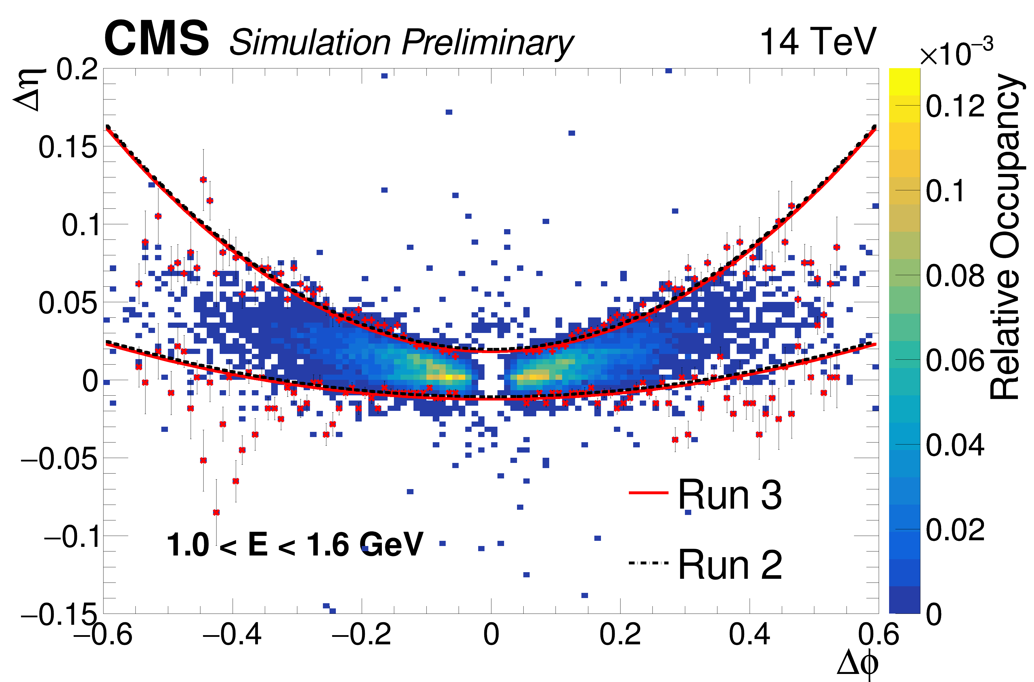
Figure 1: Shape of the SuperCluster as selected by the Mustache algorithm, obtained by accumulating many events in the bin $\eta\in[0.5,0.8]$, $E_{T}\in[1.0,1.6]$ GeV of the seed. 98% of the electromagnetic energy is contained in the Mustache area.

Being the Mustache SuperClustering a purely geometrical algorithm, it has a high signal efficiency, but it does not attempt to identify and remove clusters generated from electronics noise or from additional low energy p-p interactions overlapping in the event (pileup or PU). The increase of the pileup level and the expected increase of noise contamination during Run III of LHC due to the ECAL detector ageing, makes the development of a more performant SuperClustering algorithm based on supervised machine learning (ML) methods desirable.

The ML model architecture chosen to tackle the SuperClustering problem involves Graph Convolutional Networks (GCN) [5, 6, 7, 8] and Self-Attention (SA) layers [9, 10]. This class of models permits working on a set of related objects inferring properties about the single elements, or the overall set. One of the advantages over other architectures is that the number of objects to analyze can be different for each event. This type of architecture have also been recently explored successfully for developing a ML approximation of the full CMS PF algorithm[11].

The novel DeepSuperCluster (DeepSC) model is designed to perform three tasks at the same time: (i) SuperClustering: identify which cluster should be associated to the seed cluster to build the optimal SuperCluster; (ii) Energy regression: extract the correction factor needed to restore the generator-level particle energy. Currently this regression is trained separately on the Mustache SuperClusters to obtain the final energy estimation for ECAL calibration; (iii) Identification: classify the different types of energy deposits to discriminate between isolated electron/photon, or particles from jets. This note describes the performance of a model optimized to perform the clustering task, while the energy regression and object identification ones will be optimized in a second step.

3 DeepSC training sample and model architecture

3.1 Training sample

The model is trained on a sample of $2\cdot 10^{6}$ photons and electrons, generated uniformly in $\eta$ and $p_{T}=[1,100]$ GeV, with the full Geant4-based CMS Monte-Carlo simulation at 14 TeV. Energy deposits from noise and pileup interactions are superimposed on the signal. A pileup scenario with the number of true interactions uniformly distributed between [55,75] is used.

An optimal true association between the seeds and the clusters in the event is built by tracking the EM shower produced by original generator-level electron or photon in the Geant4 simulation, and storing the information about the amount of energy deposited in each ECAL crystal. This information allows to apply a precise matching of each cluster to the generator-level particle with energy thresholds optimized to obtain the best possible SuperCluster energy resolution, and taking fully into account effects from the energy deposition and reconstruction in the calorimeter.

The model is applied on regions of the ECAL detector around each energetic cluster ($E_{T}>1$ GeV), called seed, using the following information: (i) Energy, position and number of crystals of each cluster ; (ii) Information relative to the seed for each cluster: $\Delta\eta(\mathrm{cl},\mathrm{seed})$, $\Delta\phi(\mathrm{cl},\mathrm{seed})$, $\Delta E_{T}(\mathrm{cl},\mathrm{seed})$, $\Delta En(\mathrm{cl},\mathrm{seed})$; (ii) List of $N$ rechit information for each $i$-th cluster $[(i\eta,i\phi,iz,En)_{0},\cdots,(i\eta,i\phi,iz,En)_{N}]^{i}$; (iiii) Summary information for each region of the detector: maximum, minimum, and average of the cluster related features.

3.2 Model architecture

Fig. 2 represents the architecture of the model and the dimensions of tensors processed with it. The model is conceptually organized in four steps: encoding, graph building, graph elaboration, decoding (for each output). The model has been fully implemented in TensorFlow library version 2.3 [12].

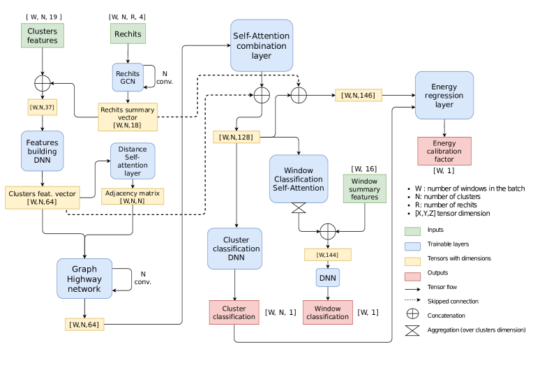
Figure 2: Schema of the DeepSC model depicting the models inputs, layers and tensors flowing through.

Encoding

A GNN layer is applied on the rechits of each cluster to obtain a single fixed-size vector representing summary rechit information for each cluster. Then, a simple feature-extracting DNN is applied on the input vector of each cluster and rechit latent vector to obtain a 64 features vector for each cluster.

Graph building

The adjacency matrix $A_{ij}$ defining the distance between each cluster is defined dynamically [5] assigning to each cluster a 3D-space coordinates vector with a SA layer and computing the Euclidean distance. Therefore, the relative importance of the interaction between the clusters, i.e. their distance in the graph, is learned automatically during the training.

Graph elaboration

A graph convolutional layer called Graph Highway Network [8] is applied on the clusters graph and then a SA layer is a applied to extract a features vector for each cluster. The application of the graph network implies a passage of information between the clusters.

Decoding

Output information is extracted from the latent space. First, a simple DNN network is applied on each cluster latent vector to get the classification output. Then, all the clusters latent vectors are combined with a different SA layer and then aggregated in a single vector to obtain the detector region classification. An energy regression layer can be applied in the same fashion.

4 Performance comparison

The performance of the DeepSC and Mustache algorithms is compared [13] in terms of the resolution of the uncorrected reconstructed SuperCluster energy $E_{\mathrm{Raw}}$ divided by the true simulated energy deposits in ECAL $E_{\mathrm{Sim}}$. The resolution is analyzed for electrons and photons versus the generator-level particle $E_{T}$ (Fig. 5), position $|\eta|$ in the detector (Fig. 5), and for different number of simulated PU vertices in the event (Fig. 5). The resolution is computed as half of the difference between the 84% quantile and the 16% quantile of the $E_{\mathrm{Raw}}/E_{\mathrm{Sim}}$ distribution in each bin.

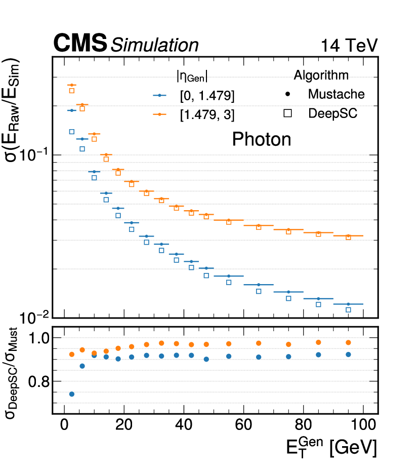
Figure 3: Comparison between the DeepSC and Mustache energy resolution in bins of generator-level particle $E_{T}^{\mathrm{Gen}}$.

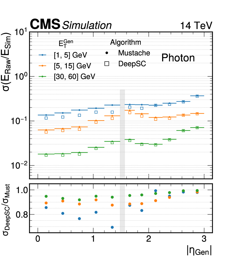
Figure 4: Comparison between the DeepSC and Mustache energy resolution in bins of generator-level particle position $|\eta|$.

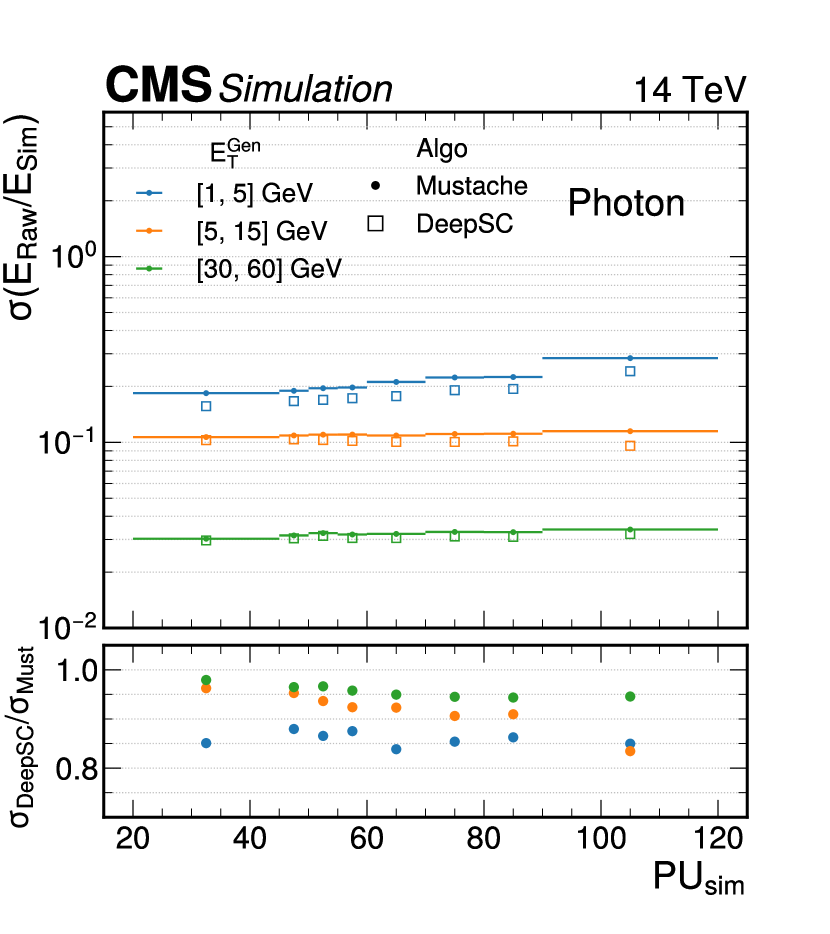
Figure 5: Comparison between the DeepSC and Mustache energy resolution in bins of number of simulated PU vertices.

The DeepSC algorithms keeps the signal efficiency similar to the Mustache one, but largely reduces the noise and PU contamination. The DeepSC largely improves the energy resolution at low energy and in the $|\eta|\in[1,2]$ region, where there are more secondary emissions at lower energy from electrons and photons, due to the higher material budget in front of ECAL. The DeepSC algorithm also makes the dependence on the energy resolution versus the number of PU vertices flatter, without using any explicit input information related to PU.

5 Conclusions

The DeepSC algorithm is a promising ML based alternative to the CMS ECAL Mustache algorithm. It is more robust against pileup and it outperforms the Mustache in terms of energy purity and capability of removing spurious energy deposits from noise and pileup, hence improving the uncorrected energy resolution of the ECAL detector.

References

References

- [1] Chatrchyan S et al. (CMS) 2008 JINST 3 S08004
- [2] 1997 CMS: The electromagnetic calorimeter Tech. Rep. CERN-LHCC-97-33, CMS-TDR-4 URL https://cds.cern.ch/record/349375
- [3] Sirunyan A M et al. (CMS) 2021 JINST 16 P05014 (Preprint 2012.06888)
- [4] Sirunyan A M et al. (CMS) 2017 JINST 12 P10003 (Preprint 1706.04965)
- [5] Shlomi J, Battaglia P and Vlimant J R 2020 (Preprint 2007.13681)
- [6] Battaglia P, Hamrick J B C, Bapst V, Sanchez A, Zambaldi V, Malinowski M, Tacchetti A, Raposo D, Santoro A and et al R F 2018 arXiv (Preprint https://arxiv.org/pdf/1806.01261.pdf)
- [7] Battaglia P W, Pascanu R, Lai M, Rezende D and Kavukcuoglu K 2016 (Preprint 1612.00222)
- [8] Xin X, Karatzoglou A, Arapakis I and Jose J M 2020 (Preprint 2004.04635)
- [9] Vaswani A, Shazeer N, Parmar N, Uszkoreit J, Jones L, Gomez A N, Kaiser L and Polosukhin I 2017 (Preprint 1706.03762)
- [10] Mikuni V and Canelli F 2021 Mach. Learn. Sci. Tech. 2 035027 (Preprint 2102.05073)
- [11] Pata J, Duarte J, Vlimant J R, Pierini M and Spiropulu M 2021 Eur. Phys. J. C 81 381 (Preprint 2101.08578)
- [12] Developers T 2021 Tensorflow Tech. rep. URL https://doi.org/10.5281/zenodo.5593257
- [13] 2021 ECAL SuperClustering with Machine Learning Tech. Rep. CERN-CMS-DP-2021-032 URL https://cds.cern.ch/record/2792321