Residue-Based Natural Language Adversarial Attack Detection

Abstract

Deep learning based systems are susceptible to adversarial attacks, where a small, imperceptible change at the input alters the model prediction. However, to date the majority of the approaches to detect these attacks have been designed for image processing systems. Many popular image adversarial detection approaches are able to identify adversarial examples from embedding feature spaces, whilst in the NLP domain existing state of the art detection approaches solely focus on input text features, without consideration of model embedding spaces. This work examines what differences result when porting these image designed strategies to Natural Language Processing (NLP) tasks - these detectors are found to not port over well. This is expected as NLP systems have a very different form of input: discrete and sequential in nature, rather than the continuous and fixed size inputs for images. As an equivalent model-focused NLP detection approach, this work proposes a simple sentence-embedding "residue" based detector to identify adversarial examples. On many tasks, it out-performs ported image domain detectors and recent state of the art NLP specific detectors .

1 Introduction

In the last decade deep learning based models have demonstrated success in a wide range of application areas, including Natural Language Processing (NLP) (Vaswani et al., 2017) and object recognition (He et al., 2015). These systems may be deployed in mission critical situations, where there is the requirement for a high level of robustness. However, Szegedy et al. (2014) demonstrated that deep models have an inherent weakness: small perturbations in the input can yield significant, undesired, changes in the output from the model. These input perturbations were termed adversarial examples and their generation adversarial attacks.

Adversarial attacks have been developed for systems operating in various domains: image systems (Serban et al., 2020; Biggio and Roli, 2017; Bhambri et al., 2019) and NLP systems (Lin et al., 2014; Samanta and Mehta, 2017; Rosenberg et al., 2017). The characteristics of the input can be very different between these application domains. Broadly, the nature of inputs can be described using two key attributes: static (fixed length) vs sequential and continuous vs discrete. Under this categorisation, image inputs are continuous and static, whilst NLP inputs are discrete and sequential. This work argues that due to the fundamental differences in the input and resulting adversarial perturbations in the different domains, adversarial attack behaviour can vary significantly from one domain to another. Hence, the extensive research on exploring and understanding adversarial perturbation behaviour in the continuous, static world of image systems does not necessarily transfer well to the NLP tasks.

For adversarial attack generation, a number of specific NLP attacks have been proposed that are designed for NLP task inputs (Lin et al., 2014; Samanta and Mehta, 2017; Rosenberg et al., 2017; Huang et al., 2018; Papernot et al., 2016; Grosse et al., 2016; Sun et al., 2018; Cheng et al., 2018; Blohm et al., 2018; Neekhara et al., 2018; Raina et al., 2020; Jia and Liang, 2017; Minervini and Riedel, 2018; Niu and Bansal, 2018; Ribeiro et al., 2018; Iyyer et al., 2018; Zhao et al., 2017). However, there has been less research on developing defence schemes. These defence strategies can be split into two main groups: model modification, where the model or data is altered at training time (e.g. adversarial training (Yoo and Qi, 2021)) and detection, where external systems or algorithms are applied to trained models to identify adversarial attacks. As model modification approaches demand re-training of models, detection approaches are usually considered easier for implementation on deployed systems and thus are often preferred. Hence, this work investigates the portability of popular detection approaches designed for image systems to NLP systems. Furthermore, this work introduces a specific NLP detection approach that exploits the discrete nature of the inputs for NLP systems. This approach out-performs standard schemes designed for image adversarial attack detection, as well as other NLP detection schemes.

The proposed NLP specific detection approach will be referred to as residue detection, as it is shown that adversarial attacks in the discrete, word sequence space result in easily detectable residual components in the sentence embedding space. This residue can be easily detected using a simple linear classifier operating in the encoder embedding space. In addition, this work shows that even when an adversary has knowledge of the linear residual detector, they can only construct attacks at a fraction of the original strength. Hence this work argues that realistic (word level, semantically similar) adversarial perturbations at the natural language input of NLP systems leave behind easily detectable residue in the sentence embedding. Interestingly, the residue detection approach is shown to perform poorly when used to detect attacks in the image domain, supporting the hypothesis that the nature of the input has an important influence on the design of effective defence strategies.

2 Related Work

Previous work in the image domain has analysed the output of specific layers in an attempt to identify adversarial examples or adversarial subspaces. First, Feinman et al. (2017) proposed that adversarial subspaces have a lower probability density, motivating the use of the Kernel Density (KD) metric to detect the adversarial examples. Nevertheless, Ma et al. (2018) found Local Intrinsic Dimensionality (LID) was a better metric in defining the subspace for more complex data. In contrast to the local subspace focused approaches of KD and LID, Carrara et al. (2019b) showed that trajectories of hidden layer features can be used to train a LSTM network to accurately discriminate between authentic and adversarial examples. Out performing all previous methods, Lee et al. (2018) introduced an effective detection framework using Mahalanobis Distance Analysis (MDA), where the distance is calculated between a test sample and the closest class-conditional Gaussian distribution in the space defined by the output of the final layer of the classifier. Li and Li (2016) also explored using the output of convolutional layers for image classification systems to identify statistics that distinguish adversarial samples from original samples. They find that by performing a PCA decomposition the statistical variation in the least principal directions is the most significant and can be used to separate original and adversarial samples. However, they argue this is ineffective as an adversary can easily suppress the tail distribution. Hence, Li and Li (2016) extract statistics from the convolutional layer output to train a cascade classifier to separate the original and adversarial samples. Most recently, Mao et al. (2019) avoid the use of artificially designed metrics and combine the adversarial subspace identification stage and the detecting adversaries stage into a single framework, where a parametric model adaptively learns the deep features for detecting adversaries.

In contrast to the embedding space detection approaches, Cohen et al. (2019) shows that influence functions combined with Nearest Neighbour distances perform comparably or better than the above standard detection approaches. Other detection approaches have explored the use of uncertainty: Smith and Gal (2018) argues that adversarial examples are out of distribution and do not lie on the manifold of real data. Hence, a discriminative Bayesian model’s epistemic (model) uncertainty should be high. Therefore, calculations of the model uncertainty are thought to be useful in detecting adversarial examples, independent of the domain. However, Bayesian approaches aren’t always practical in implementation and thus many different approaches to approximate this uncertainty have been suggested in literature (Leibig et al., 2017; Gal, 2016; Gal and Ghahramani, 2016).

There are a number of existing NLP specific detection approaches. For character level attacks, detection approaches have exploited the grammatical (Sakaguchi et al., 2017) and spelling (Mays et al., 1991; Islam and Inkpen, 2009) inconsistencies to identify and detect the adversarial samples. However, these character level attacks are unlikely to be employed in practice due to the simplicity with which they can be detected. Therefore, detection approaches for the more difficult semantically similar attack samples are of greater interest, where the meaning of the textual input is maintained without compromising the spelling or grammatical integrity. To tackle such word-level, semantically similar examples, Zhou et al. (2019) designed a discriminator to classify each token representation as part of an adversarial perturbation or not, which is then used to ‘correct’ the perturbation. Other detection approaches (Raina et al., 2020; Han et al., 2020; Minervini and Riedel, 2018) have shown some success in using perplexity to identify adversarial textual examples. Most recently, Mozes et al. (2020) achieved state of the art performance with the Frequency Guided Word Substitution (FGWS) detector, where a change in model prediction after substituting out low frequency words is revealing of adversarial samples.

3 Adversarial Attacks

An adversarial attack is defined as an imperceptible change to the input that causes an undesired change in the output of a system. Often, an attack is found for a specific data point, $\mathbf{x}$. Consider a classifier $\mathcal{F}_{\hat{\theta}}$, with parameters $\hat{\theta}$, that predicts a class label for an input data point, $\mathbf{x}$, sampled from the input distribution $\mathcal{X}$. A successful adversarial attack is where a perturbation $\bm{\delta}$ at the input causes the system to miss-classify,

$$\mathcal{F}_{\hat{\theta}}(\mathbf{x}+\bm{\delta})\neq\mathcal{F}_{\hat{\theta}}(\mathbf{x}).$$ (1)

When defining adversarial attacks, it is important consider the interpretation of an imperceptible change. Adversarial perturbations are not considered effective if they are easy to detect. Hence, the size of the perturbation must be constrained:

$$\mathcal{G}(\mathbf{x},\mathbf{x}+\bm{\delta})\leq\epsilon,$$ (2)

where the function $\mathcal{G}()$ describes the form of constraint and $\epsilon$ is a selected threshold of imperceptibility. Typically, when considering continuous space inputs (such as images), a popular form of the constraint of Equation 2, is to limit the perturbation in the $l_{p}$ norm, with $p\in[1,\infty)$, e.g. $||\bm{\delta}||_{p}\leq\epsilon$.

For whitebox attacks in the image domain, the dominant attack approach has proven to be Projected Gradient Descent (PGD) (Kurakin et al., 2016). The PGD approach, iteratively updates the adversarial perturbation, $\bm{\delta}$, initialised as $\bm{\delta}_{0}=\mathbf{0}$. Each iterative step moves the perturbation in the direction that maximises the loss function, $\mathcal{L}$, used in the training of the model,

$$\bm{\delta}_{i+1}=\texttt{clip}_{\epsilon}(\bm{\delta}_{i}+\alpha\nabla_{\bm{\delta}_{i}}\mathcal{L}(\mathbf{x}+\bm{\delta}_{i};\hat{\theta})),$$ (3)

where $\alpha$ is an arbitrary step-size parameter and the clipping function, $\texttt{clip}_{\epsilon}$, ensures the imperceptibility constraint of Equation 2 is satisfied.

When considering the NLP domain, a sequential, discrete input of $L$ words, can be explicitly represented as,

$$\mathbf{x}=w_{1:L}=w_{1},w_{2},\ldots,w_{L-1},w_{L},$$ (4)

where, the discrete word tokens, $w_{1:L}$, are often mapped to a continuous, sequential word embedding (Devlin et al., 2019) space,

$$\mathbf{h}_{1:L}=\mathbf{h}_{1},\mathbf{h}_{2},\ldots,\mathbf{h}_{L-1},\mathbf{h}_{L}.$$ (5)

Attacks must take place in the discrete text space,

$$\mathbf{x}+\bm{\delta}=w^{\prime}_{1:L^{\prime}}=w^{\prime}_{1},w^{\prime}_{2},\ldots,w^{\prime}_{L^{\prime}-1},w_{L^{\prime}}.$$ (6)

This requires a change in the interpretation of the perturbation $\bm{\delta}$. It is not simple to define an appropriate function ${\cal G}()$ in Equation 2 for word sequences. Perturbations can be measured at a character or word level. Alternatively, the perturbation could be measured in the vectorized embedding space (Equation 5), using for example $l_{p}$-norm based (Goodfellow et al., 2015) metrics or cosine similarity (Carrara et al., 2019a), which have been used in the image domain. However, constraints in the embedding space do not necessarily achieve imperceptibility in the original word sequence space. The simplest approach is to use a variant of an edit-based measurement (Li et al., 2018), ${\cal L}_{\tt e}()$, which counts the number of changes between the original sequence, $w_{1:L}$ and the adversarial sequence $w^{\prime}_{1:L^{\prime}}$, where a change is a swap/addition/deletion, and ensures it is smaller than a maximum number of changes, $N$,

$${\cal L}_{\tt e}(w_{1:L},w^{\prime}_{1:L^{\prime}})\leq N.$$ (7)

For the NLP adversarial attacks this work only examines word-level attacks, as these are considered more difficult to detect than character-level attacks. As an example, for an input sequence of $L$ words, a $N$-word substitution adversarial attack, $w^{\prime}_{1:N}$, applied at word positions $n_{1},n_{2},\ldots,n_{N}$ gives the adversarial output, $w^{\prime}_{1:L^{\prime}}$

$$w^{\prime}_{1:L^{\prime}} =w_{1},\ldots,w_{n_{1}-1},w^{\prime}_{1},w_{n_{1}+1},\ldots,$$

$$\hskip 10.00002ptw_{n_{N}-1},w^{\prime}_{N},w_{n_{N}+1},\ldots,w_{L}.$$ (8)

The challenge is to select which words to replace, and what to replace them with. A simple yet effective substitution attack approach that ensures a small change in the semantic content of a sentence is to use saliency to rank the word positions, and to use word synonyms for the substitutions (Ren et al., 2019). This attack is termed Probability Weight Word Saliency (PWWS). The highest ranking word word can be swapped for a synonym from a pre-selected list of given synonyms. The next most highly ranked word is substituted in the same manner and the process is repeated till the required $N$ words have been substituted.

The above approach is limited to attacking specific word sequences and so cannot easily be generalised to universal attacks (Moosavi-Dezfooli et al., 2016), where the same perturbation is used for all inputs. For this situation, a simple solution is concatenation (Wang and Bansal, 2018; Blohm et al., 2018), where for example, the same $N$-length sequence of words is appended to each input sequence of words, as described in Raina et al. (2020). Here,

$$w^{\prime}_{1:L^{\prime}}=w_{1},\ldots,w_{L},w^{\prime}_{1},\ldots,w^{\prime}_{N}.$$ (9)

In both the substitution attack (Equation 3) and the concatenation attack (Equation 9), the size of the attack can be measured using the number of edits, ${\cal L}_{\tt e}(w_{1:L},w^{\prime}_{1:L^{\prime}})=N$.

4 Adversarial Attack Detection

For a deployed system, the easiest approach to defend against adversarial attacks is to use a detection process to identify adversarial examples without having to modify the existing system.

For the image domain Section 2 discusses many of the standard detection approaches. In this work, we select two distinct approaches that have been generally successful: uncertainty (Smith and Gal, 2018), where adversarial samples are thought to result in greater epistemic uncertainty and Mahalanobis Distance (Lee et al., 2018), where the Mahalanobis distance in the embedding space is indicative of how out of distribution a sample is (adversarial samples are considered more out of distribution). In the NLP domain, when excluding trivial grammar and spelling based detectors, perplexity based detectors can be used (Raina et al., 2020). Many other NLP specific detectors (Zhou et al., 2019; Han et al., 2020; Minervini and Riedel, 2018) have been proposed, but Mozes et al. (2020)’s FGWS detector is considered the state of art and is thus selected for comparison. Here low frequency words in an input are substituted for higher frequency words and the change in model prediction is measured - adversarial samples are found to generally have a greater change. This work introduces a further NLP specific detector: residue detection, described in detail in Section 4.1.

When considering any chosen detection measure $\mathcal{F}_{\tt d}$, a threshold $\beta$ can be selected to decide whether an input, $w_{1:L}$, is adversarial or not, where ${\cal F}_{\tt d}(w_{1:L})>\beta$, implies that $w_{1:L}$ is an adversarial sample. To assess the success of the adversarial attack detection processes, precision-recall curves are used. For the binary classification task of identifying an input as adversarially attacked or not, at a given threshold $\beta$, the precision and recall values can be computed as $\text{prec}=\text{TP}/\text{TP}+\text{FP}$ and $\text{rec}=\text{TP}/\text{TP}+\text{FN}$, where TP, FP and FN are the standard true-positive, false-positive and false-negative definitions. A single point summary of precision-recall curves is given with the F₁ score.

4.1 Residue Detection

In this work we introduce a new NLP detection approach, residue detection, that aims to exploit the nature of the NLP input space, discrete and sequential. Here we make two hypotheses:

1. Adversarial samples in an encoder embedding space result in larger components (residue) in central PCA eigenvector components than original examples.

2. The residue is only significant (detectable) for systems operating on discrete data (e.g. NLP systems).

The rationale behind these hypotheses is discussed next.

Deep learning models typically consist of many layers of non-linear activation functions. For example, in the NLP domain systems are usually based on layers of the Transformer architecture (Vaswani et al., 2017). The complete end-to-end model $\mathcal{F}_{\hat{\theta}}()$ can be treated as a two stage process, with an initial set of layers forming the encoding stage, $\mathcal{F}_{\tt en}()$ and the remaining layers forming the output stage, $\mathcal{F}_{\tt cl}()$, i.e. $F_{\hat{\theta}}(\mathbf{x})=\mathcal{F}_{\tt cl}\left(\mathcal{F}_{\tt en}(\mathbf{x})\right)$.

If the encoding stage of the end-to-end classifier is sufficiently powerful, then the embedding space $\mathcal{F}_{\tt en}(\mathbf{x})$ will have compressed the useful information into very few dimensions, allowing the output stage to easily separate the data points into classes (for classification) or map the data points to a continuous value (for regression). A simple Principal Component Analysis (PCA) decomposition of this embedding space can be used to visualize the level of compression of the useful information. The PCA directions can be found using the eigenvectors of the covariance matrix, $\mathbf{C}$, of the data in the encoder embedding space. If $\{\mathbf{q}_{i}\}_{i=1}^{d}$, where $d$ is the dimension of the encoder embedding space, represent the eigenvectors of $\mathbf{C}$ ordered in descending order by the associated eigenvalue in magnitude, then it is expected that almost all useful information is contained within the first few principal directions, $\{\mathbf{q}_{i}\}_{i=1}^{p}$, where $p\ll d$. Hence, the output stage, $\mathcal{F}_{\tt cl}()$ will implicitly use only these useful components. The impact of a successful adversarial perturbation, $\mathcal{F}_{\tt en}(\mathbf{x}+\bm{\delta})$, is the significant change in the components in the principal eigenvector directions $\{\mathbf{q}_{i}\}_{i=1}^{p}$, to allow fooling of the output stage. Due to the complex nature of the encoding stage and the out of distribution nature of the adversarial perturbations, there are likely to be residual components in the non-principal $\{\mathbf{q}_{i}\}_{i=p+1}^{d}$ eigenvector directions. These perturbations in the non-principal directions are likely to be more significant for the central eigenvectors, as the encoding stage is likely to almost entirely compress out components in the least principal eigenvector directions, $\{\mathbf{q}_{i}\}_{i=d^{\prime}+1}^{d}$, where $d^{\prime}\approx d$. Hence, $\{\mathbf{q}_{i}\}_{i=p+1}^{d^{\prime}}$ can be viewed as a subspace containing adversarial attack residue that can be used to identify adversarial examples.

The existence of adversarial attack residue in the central PCA eigenvector directions, $\{\mathbf{q}_{i}\}_{i=p+1}^{d^{\prime}}$, suggests that in the encoder embedding space, $\mathcal{F}_{\tt en}(\mathbf{x})$, adversarial and original examples are linearly separable. This motivates the use of a simple linear classifier as an adversarial attack detector,

$$P(\text{adv}|\mathbf{x})=\sigma(\mathbf{W}\mathcal{F}_{\tt en}(\mathbf{x})+b),$$ (10)

where $\mathbf{W}$ and $b$ are the parameters of the linear classifier to be learnt and $\sigma$ is the sigmoid function.

The above argument cannot predict how significant the residue in the central eigenvector space is likely to be. For the discrete space NLP attacks, the input perturbations are semantically small, whilst for continuous space image attacks the perturbations are explicitly small using a standard $l_{p}$-norm. Hence, it is hypothesised that NLP perturbations cause larger errors to propagate through the system, resulting in more significant residue in the encoder embedding space than that for image attacks. Thus, the residue technique is only likely to be a feasible detection approach for discrete text attacks.

The hypotheses made in this section are analysed and empirically verified in Section 5.3.

5 Experiments

5.1 Experimental Setup

Table 1 describes four NLP classification datasets: IMDB (Maas et al., 2011); Twitter (Saravia et al., 2018); AG News (Zhang et al., 2015) and DBpedia (Zhang et al., 2015). Further, a regression dataset, Linguaskill-Business (L-Bus) (Chambers and Ingham, 2011) is included. The L-Bus data is from a multi-level prompt-response free speaking test i.e. candidates from a range of proficiency levels provide open responses to prompted questions. Based on this audio input a system must predict a score of 0-6 corresponding to the 6 CEFR (Council of Europe, 2001) grades. This audio data was transcribed using an Automatic Speech Recognition system with an average word error rate of 19.5%.

Dataset	#Train	#Test	#Classes
IMDB	25,000	25,000	2
Twitter	16,000	2000	6
AG News	120,000	7600	4
DBpedia	560,000	70,000	14
L-Bus	900	202	1

Table 1: NLP Datasets.

All NLP task models were based on the Transformer encoder architecture (Vaswani et al., 2017). Table 2 indicates the specific architecture used for each task and also summarises the classification and regression performance for the different tasks. For classification tasks, the performance is measured by top 1 accuracy, whilst for the regression task (L-Bus), the performance is measured using Pearson Correlation Coefficient (PCC).

Dataset	Transformer	Performance
IMDB	BERT	Acc: 93.8%
Twitter	ELECTRA	Acc: 93.3%
AG News	BERT	Acc: 94.5%
DBpedia	ELECTRA	Acc: 99.2%
L-Bus	BERT	PCC: 0.749

Table 2: Performance of models (BERT (Devlin et al., 2018), ELECTRA (Clark et al., 2020)).

Table 3 shows the impact of realistic adversarial attacks on the tasks: substitution (sub) attack (Equation 3), which replaces the $N$ most salient tokens with a synonym defined by WordNet, as dictated by the PWWS attack algorithm described in Section 3; or a targeted universal concatenation (con) attack (Equation 9), used for the regression task on the L-Bus dataset, seeking to maximise the average score output from the system by appending the same $N$ words to the end of each input. For classification tasks, the impact of the adversarial attack is measured using the fooling rate, the fraction of originally correctly classified points, misclassified after the attack, whilst for the regression task, the impact is measured as the average increase in the output score.

Dataset	Attack	$N$	Impact
IMDB	sub	25	Fool: 0.70
Twitter	sub	6	Fool: 0.77
AG News	sub	40	Fool: 0.65
DBpedia	sub	25	Fool: 0.52
L-Bus	con	3	Score: $+0.51$

Table 3: Impact of different $N$-word adversarial attacks.

5.2 Results

Section 4.1 predicts that adversarial attacks in the discrete text space leave residue in a system’s encoder embedding space that can be detected using a simple linear classifier. Hence, using the 12-layer Transformer encoder’s output CLS token embedding as the encoder embedding space for each dataset’s trained system (Table 2), a simple linear classifier, as given in Equation 10, was trained  to detect adversarial examples from the adversarial attacks given for each dataset in Table 3. The training of the detection linear classifier was performed on the training data (Table 1) augmented with an equivalent adversarial example for each original input sample in the dataset. Using the test data samples augmented with adversarial examples (as defined by Table 3), Table 4 compares the efficacy of the linear residue detector to other popular detection strategies  (from Section 4) using the best F₁ score. It is evident from the high F-scores, that for most NLP tasks the linear detection approach is better than other state of the art NLP specific and ported image detection approaches.

Dataset	Res	Perp	FGWS	MD	Unc
IMDB	0.91	0.68	0.87	0.77	0.75
Twitter	0.84	0.67	0.76	0.77	0.78
AG News	0.95	0.69	0.89	0.78	0.75
DBpedia	0.80	0.67	0.82	0.78	0.90
L-Bus	0.99	0.68	0.91	0.75	0.81

Table 4: F₁-score performance of detection approaches.

However, an adversary may have knowledge of the detection approach and may attempt to design an attack that directly avoids detection. Hence, for each dataset, the attack approaches were repeated with the added constraint that any attack words that resulted in detection were rejected. The impact of attacks that suppress detection have been presented in Table 5. Generally, it is shown across all NLP tasks that an adversary that attempts to avoid detection of its residue by a previously trained linear classifier, can only generate a significantly less powerful adversarial attack.

Dataset	Without	With
IMDB	0.70	0.19
Twitter	0.77	0.23
AG News	0.65	0.16
DBpedia	0.52	0.14
L-Bus	$+0.51$	$+0.23$

Table 5: Fooling rate (classification) or score (regression) with and without attack modified to avoid detection.

5.3 Analysis

The aim of this section is verify that the success of the residue detector can be explained by the two main hypotheses made in Section 4.1. The claim that residue is left by adversarial samples in the central PCA eigenvector components is explored first. For each NLP task a PCA projection matrix is learnt in the encoder embedding space using the original training data samples (Table 1). Using the test data, the residue in the embedding space can be visualized through a plot of the average (across the data) component, $\rho_{i}=\frac{1}{J}\sum_{j=1}^{J}\rho_{i,j}$ in each eigenvector direction, $\mathbf{q}_{i}$ of the original and attacked data, where

$$\rho_{i,j}=\left|\mathcal{F}_{\tt en}(\mathbf{x}_{j})^{\tt T}\mathbf{q}_{i}\right|,$$ (11)

with $\mathbf{x}_{j}$ being the $j$th data point. Figure 1 shows an example plot for the Twitter dataset, where $\rho_{i}$ is plotted against the eigenvalue rank, $i$ for the original and attacked data examples. Residue plots for other datasets are included in Appendix A. Next, it is necessary to verify that the residue detector specifically uses the residue in the central eigenvector components to distinguish between original and adversarial samples. To establish this, each encoder embedding, $\mathcal{F}_{\tt{en}}(x)$’s components not within a target subspace of PCA eigenvector directions $\{\mathbf{q}_{i}\}_{i=p}^{p+w}$, are removed, i.e. we have a projected embedding, $\mathbf{x}^{(\text{p})}=F_{\tt{en}}(x)-\sum_{i\notin[p,p+w)}\mathbf{q}_{i}^{T}F_{\tt{en}}(x)\mathbf{q}_{i}$, where $w$ is a window size to choose. Now, using $\mathcal{F}_{\tt{cl}}(\mathbf{x}^{(\text{p})})$ and a residue detector trained using the modified embeddings, $\mathbf{x}^{(\text{p})}$, the classifier’s ($\mathcal{F}_{\tt{cl}}(\mathbf{x}^{(\text{p})})$) accuracy and detector performance (measured using F1 score) can be found. Figure 2 shows the performance of the classifier ($\mathcal{F}_{\tt{cl}}(\mathbf{x}^{(\text{p})})$) and the detector for different start components $p$, with the window size, $w=5$. It is clear that the principal components hold the most important information for classifier accuracy, but, as hypothesised in Section 4.1, it is the more central eigenvector components that hold the most information useful for the residue detector, i.e. the subspace defined by $\{\mathbf{q}_{i}\}_{i=5}^{10}$ holds the most detectable residue from adversarial examples.

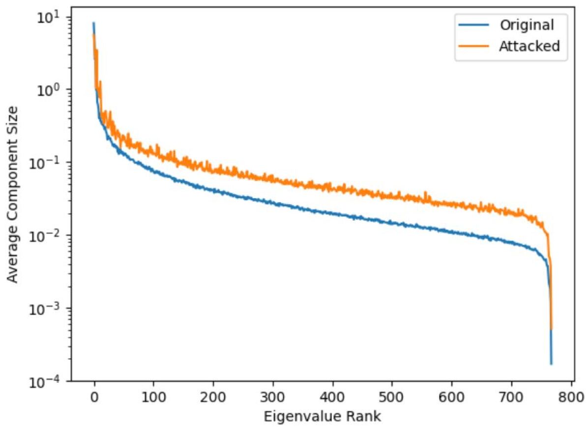
Figure 1: Encoder Embedding Space Residue Plot.

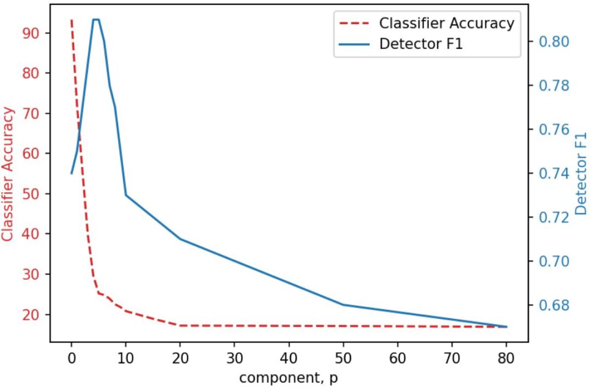
Figure 2: Performance of classifier and detector with windowed projection of encoder embedding space.

The second hypothesis in Section 4.1 claims that the existence of residue in the central eigenvector components is due to the discrete nature of NLP adversarial attacks. Hence, to analyze the impact of the discrete aspect of the attack, an artificial continuous space attack was constructed for the Twitter NLP system, where the continuous input embedding layer space (Equation 5) of the system is the space in which the attack is performed. Using the Twitter emotion classifier, a PGD (Equation 3) attack was performed on the input embeddings for each token, where the perturbation size was limited to be $\epsilon=0.1$ in the l_∞ norm, achieving a fooling rate of 0.73. Note that this form of attack is artificial, as a real adversary can only modify the discrete word sequence (Equation 4). To compare the influence of discrete and continuous attacks on the same system, the average (across dataset) l₂ and l_∞ norms of the perturbations in the input layer embedding space were found. Further, a single value summary, $N_{\sigma}$, of the residue plot (e.g. Figure 1), was calculated for each attack. $N_{\sigma}$ is the average difference in standard deviations between the original component mean, $\rho_{i}^{\text{(orig)}}$ and attack mean, $\rho_{i}^{\text{(attack)}}$,

$$N_{\sigma}=\frac{1}{I}\sum_{i=1}^{I}\frac{\left|\rho_{i}^{\text{(attack)}}-\rho_{i}^{\text{(orig)}}\right|}{\sqrt{\textrm{Var}_{j}[\rho_{i,j}^{\text{(orig)}}]}}.$$ (12)

Table 6 reports these metrics for the discrete and artificial continuous NLP adversarial attacks on the Twitter system . It is apparent that perturbation sizes for the discrete attacks are significantly larger. Moreover, $N_{\sigma}$ is significantly smaller for the continuous space attack, indicating that the residue left by continuous space adversarial attacks is smaller.

Attack	$N_{\sigma}$	l2 error	l∞ error
Discrete	1.201	$50.2_{\pm 19.2}$	$3.26_{\pm 0.86}$
Continuous	0.676	$5.35_{\pm 3.95}$	$0.08_{\pm 0.03}$

Table 6: Comparison of token level discrete attack and input embedding layer continuous PGD attack.

To explicitly observe the impact of the nature of data on detectors, adversarial attacks are considered in four domains: the discrete, sequential NLP input space (NLP-disc); the artificial continuous, sequential embedding space of an NLP model (NLP-cont); the continuous, static image input space (Img-cont) and a forced discretised, static image input space (Img-disc). For the NLP-disc and NLP-cont the same attacks as in Table 6 are used. For the continuous image domain (Img-cont), a VGG-16 architecture image classifier trained on CIFAR-100 (Krizhevsky et al., 2009) image data (achieving a top-5 accuracy of 90.1%) and attacked using a standard l_∞ PGD approach (Equation 3) is used. For the discrete image domain (Img-disc), the CIFAR-100 images, $\mathbf{X}\in\mathbb{Z}_{256}^{R\times R}$ were discretised using function $\mathcal{Q}_{q}:\mathbb{Z}_{256}^{R\times R}\to\mathbb{Z}_{q}^{R\times R}$, where $\mathbb{Z}_{q}=\{0,1\frac{256}{q-1},2\frac{255}{q-1},\ldots,255\}$. In this work 2-bit quantization was used, i.e. $q=4$. With this quantization, a VGG-16 architecture was trained to achieve 78.2% top-5 accuracy. To perform a discrete space attack, a variant of the PWWS synonym substitution attack (Section 3) was implemented, where synonyms were interpreted as closest permitted quantisation values and $N$ pixel values were substituted. For these different domains, Table 7 compares applicable detection approaches (certain NLP detection approaches are not valid outside the word sequence space) using the best F₁ score, where different attack perturbation sizes are considered ($N$ substitutions for discrete attacks and for continuous attacks $|\bm{\delta}|\leq\epsilon$ for perturbation $\bm{\delta}$).

Domain	Attack	Res	Unc	MD
NLP-disc	$N$=3	0.80	0.74	0.73
	$N$=6	0.84	0.78	0.77
NLP-cont	$\epsilon$=0.1	0.67	0.71	0.70
	$\epsilon$=0.3	0.67	0.80	0.85
Img-disc	$N$=200	0.78	0.67	0.70
	$N$=400	0.84	0.68	0.72
Img-cont	$\epsilon$=12	0.68	0.70	0.72
	$\epsilon$=48	0.83	0.81	0.87

Table 7: Portability of detection approaches.

In the discrete domains, the residue detection approach is better than all the other approaches. However, in the continuous data type domains, the Mahalanobis Distance dominates as the detection approach, with the residue detection approach performing the worst. As predicted by the second hypothesis of Section 4.1, the lack of success of the residue detection approach is expected here - the residue detection approach is only successful for discrete space attacks.

To verify that the residue detection approach is agnostic to the type of attack, the residue detector trained on substitution attack examples was evaluated on concatenation attack examples. Using the Twitter dataset, a $N=3$ concatenation attack was applied, achieving a fooling rate of 0.59. In this setting, the residue detector (trained on the $N=6$ substitution adversarial examples) achieved a F₁ score of 0.81, which is comparable to the original score of 0.84 (from Table 4). This shows that even with different attack approaches similar forms of residue are produced, meaning a residue detector can be used even without knowledge of the type of adversarial attack.

6 Conclusions

In recent years, deep learning systems have been deployed for a large number of tasks, ranging from the image to the natural language domain. However, small, imperceptible adversarial perturbations at the input, have been found to easily fool these systems, compromising their validity in high-stakes applications. Defence strategies for deep learning systems have been extensively researched, but this research has been predominantly carried out for systems operating in the image domain. As a result, the adversarial detection strategies developed, are inherently tuned to attacks on the continuous space of images. This work shows that these detection strategies do not necessarily transfer well to attacks on natural language processing systems. Hence, an adversarial attack detection approach is proposed that specifically exploits the discrete nature of perturbations for attacks on discrete sequential inputs.

The proposed approach, termed residue detection, demonstrates that imperceptible attack perturbations on natural language inputs tend to result in large perturbations in word embedding spaces, which result in distinctive residual components. These residual components can be identified using a simple linear classifier. This residue detection approach was found to out-perform both detection approaches ported from the image domain and other state of the art NLP specific detectors.

The key finding in this work is that the nature of the data (e.g. discrete or continuous) strongly influences the success of detection systems and hence it is important to consider the domain when designing defence strategies.

7 Limitations, Risks and Ethics

A limitation of the residue approach proposed in this work is that it requires training on adversarial examples, which is not necessary for other NLP detectors. This means there is a greater computational cost associated with this detector. Moreover, associated with this limitation is a small risk, where in process of generating creative adversarial examples to build a robust residue detector, the attack generation scheme may be so strong that it can more easily evade detection from other existing detectors already deployed in industry. There are no further ethical concerns related to this detector.

8 Acknowledgements

This paper reports on research supported by Cambridge Assessment, University of Cambridge. Thanks to Cambridge English Language Assessment for support and access to the Linguaskill-Business data. The authors would also like to thank members of the ALTA Speech Team.

Appendix Appendix A

Training Details

For each NLP dataset, pre-trained base (12-layer, 768-hidden dimension, 110M parameters) Transformer encoders  were fine-tuned during training. Table A.1 gives the training hyperparameters: learning rate (lr), batch size (bs) and the number of training epochs. In all training regimes an Adam optimizer was used. With respect to hardware, NVIDIA Volta GPU cores were used for training all models.

Dataset	Model	lr	bs	epochs
IMDB	BERT	1e-5	8	2
Twitter	ELECTRA	1e-5	8	2
AG News	BERT	1e-5	8	2
DBpedia	ELECTRA	1e-5	8	2
L-Bus	BERT	1e-6	16	5

Table A.1: Training Hyperparameters

Experiments

Figure A.1 presents the impact of adversarial attacks of different perturbation sizes, $N$ on each NLP dataset. All classification datasets’ models underwent saliency ranked, $N$-word substitution attacks described in Equation 3, whilst the regression dataset, L-Bus, was subject to a $N$-word concatenation attack as in Equation 9. For the classification tasks the impact of the adversarial attacks was measured using fooling rate, whilst for the L-Bus dataset task, the average output score from the system is given. Figure A.2 gives the encoder embedding space PCA residue plots for all the datasets not included in the main text.

Table A.2 compares the impact on error sizes (using $l_{2}$ and $l_{\infty}$ norms) and the residue plot metric, $N_{\sigma}$ for the original text space discrete attacks and an artificial input embedding space continuous attack. The purpose of this table is to present the results for the datasets not included in the main text in Table 6.

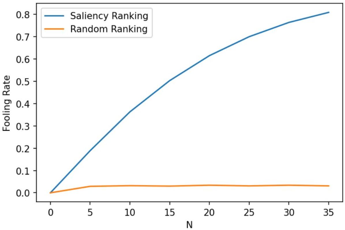
(a) IMDB

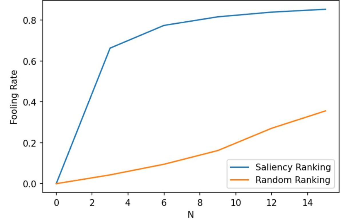
(b) Twitter

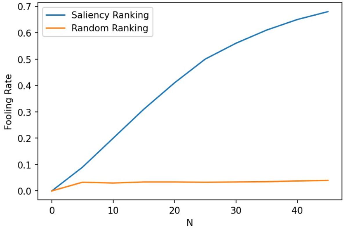
(c) AG News

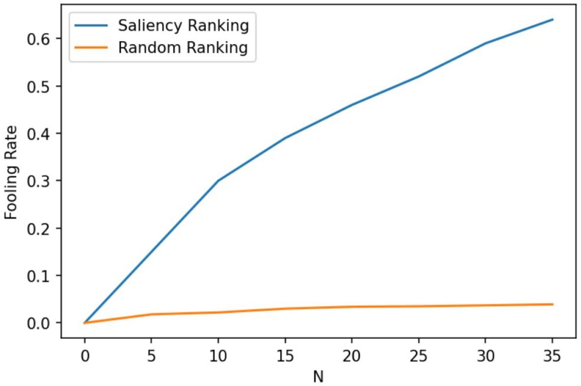
(d) DBpedia

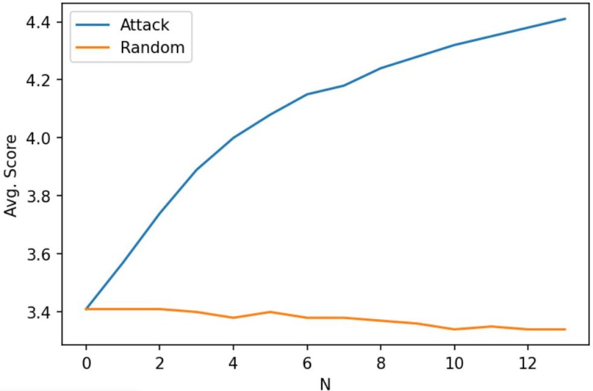
(e) L-Bus

Figure A.1: Adversarial Attack Impact against $N$-word attack.

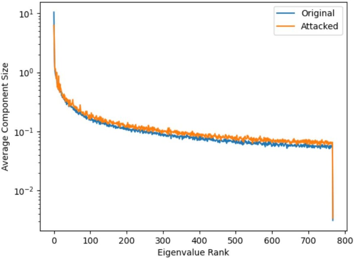
(a) IMDB

(b) Twitter

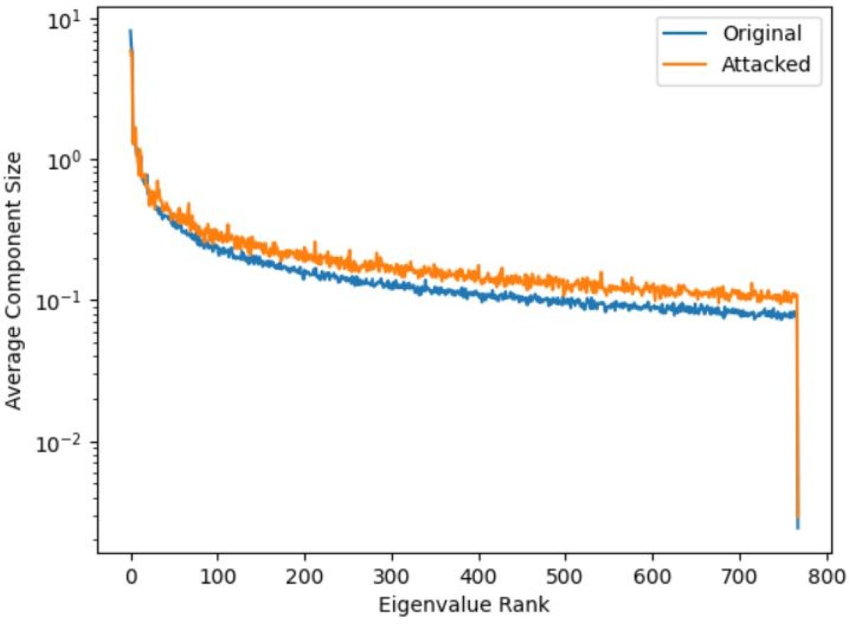
(c) AG News

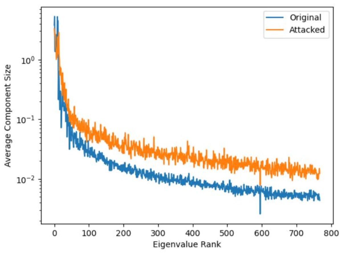
(d) DBpedia

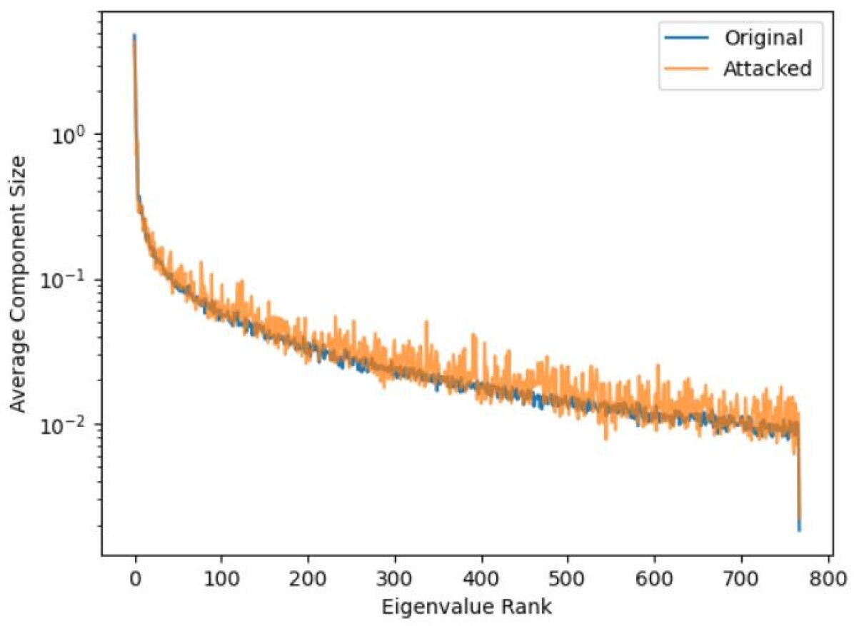
(e) L-Bus

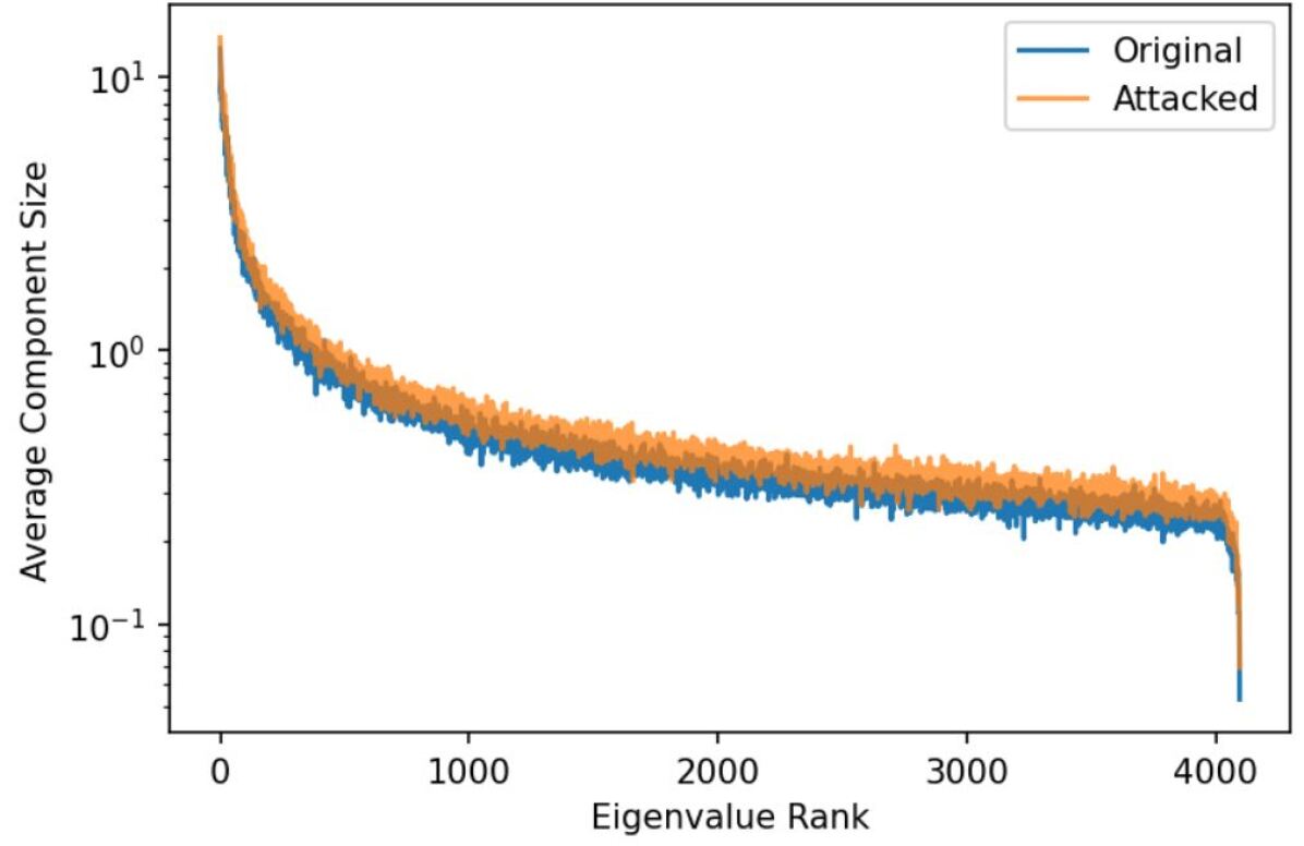
(f) CIFAR-100

Figure A.2: Encoder Embedding space residue plot using PCA decomposition.

Dataset	Attack	$N_{\sigma}$	$l_{2}$ error	$l_{\infty}$ error
IMDB	Discrete	0.181	$73.5_{\pm 22.5}$	$4.02_{\pm 0.95}$
	Continuous	0.111	$6.73_{\pm 3.98}$	$0.09_{\pm 0.03}$
Twitter	Discrete	1.201	$50.2_{\pm 19.2}$	$3.26_{\pm 0.86}$
	Continuous	0.676	$5.35_{\pm 3.95}$	$0.08_{\pm 0.03}$
AG News	Discrete	0.642	$67.9_{\pm 28.1}$	$3.35_{\pm 0.95}$
	Continuous	0.393	$5.41_{\pm 4.10}$	$0.09_{\pm 0.04}$
DBpedia	Discrete	1.355	$57.4_{\pm 18.6}$	$3.29_{\pm 0.88}$
	Continuous	0.991	$6.57_{\pm 3.23}$	$0.09_{\pm 0.04}$
L-Bus	Discrete	0.201	$94.6_{\pm 30.1}$	$5.91_{\pm 1.12}$
	Continuous	0.135	$8.22_{\pm 3.54}$	$0.07_{\pm 0.04}$

Table A.2: Comparison of token level discrete attack and input embedding layer continuous PGD attack.

References

- Bhambri et al. (2019) Siddhant Bhambri, Sumanyu Muku, Avinash Tulasi, and Arun Balaji Buduru. 2019. A study of black box adversarial attacks in computer vision. CoRR, abs/1912.01667.
- Biggio and Roli (2017) Battista Biggio and Fabio Roli. 2017. Wild patterns: Ten years after the rise of adversarial machine learning. CoRR, abs/1712.03141.
- Blohm et al. (2018) Matthias Blohm, Glorianna Jagfeld, Ekta Sood, Xiang Yu, and Ngoc Thang Vu. 2018. Comparing attention-based convolutional and recurrent neural networks: Success and limitations in machine reading comprehension. CoRR, abs/1808.08744.
- Carrara et al. (2019a) Fabio Carrara, Rudy Becarelli, Roberto Caldelli, Fabrizio Falchi, and Giuseppe Amato. 2019a. Adversarial examples detection in features distance spaces. In Computer Vision – ECCV 2018 Workshops, pages 313–327, Cham. Springer International Publishing.
- Carrara et al. (2019b) Fabio Carrara, Rudy Becarelli, Roberto Caldelli, Fabrizio Falchi, and Giuseppe Amato. 2019b. Adversarial Examples Detection in Features Distance Spaces: Subvolume B, pages 313–327. ECCV.
- Chambers and Ingham (2011) Lucy Chambers and Kate Ingham. 2011. The BULATS online speaking test. Research Notes, 43:21–25.
- Chen et al. (2016) X. Chen, X. Liu, Y. Qian, M. J. F. Gales, and P. C. Woodland. 2016. Cued-rnnlm — an open-source toolkit for efficient training and evaluation of recurrent neural network language models. In 2016 IEEE International Conference on Acoustics, Speech and Signal Processing (ICASSP), pages 6000–6004.
- Cheng et al. (2018) Minhao Cheng, Jinfeng Yi, Huan Zhang, Pin-Yu Chen, and Cho-Jui Hsieh. 2018. Seq2sick: Evaluating the robustness of sequence-to-sequence models with adversarial examples. CoRR, abs/1803.01128.
- Clark et al. (2020) Kevin Clark, Minh-Thang Luong, Quoc V. Le, and Christopher D. Manning. 2020. ELECTRA: pre-training text encoders as discriminators rather than generators. CoRR, abs/2003.10555.
- Cohen et al. (2019) Gilad Cohen, Guillermo Sapiro, and Raja Giryes. 2019. Detecting adversarial samples using influence functions and nearest neighbors. CoRR, abs/1909.06872.
- Council of Europe (2001) Council of Europe. 2001. Common European Framework of Reference for Languages: Learning, Teaching, Assessment. Cambridge University Press.
- Devlin et al. (2018) Jacob Devlin, Ming-Wei Chang, Kenton Lee, and Kristina Toutanova. 2018. BERT: pre-training of deep bidirectional transformers for language understanding. CoRR, abs/1810.04805.
- Devlin et al. (2019) Jacob Devlin, Ming-Wei Chang, Kenton Lee, and Kristina Toutanova. 2019. Bert: Pre-training of deep bidirectional transformers for language understanding.
- Feinman et al. (2017) Reuben Feinman, Ryan R. Curtin, Saurabh Shintre, and Andrew B. Gardner. 2017. Detecting adversarial samples from artifacts.
- Gal (2016) Y. Gal. 2016. Uncertainty in deep learning.
- Gal and Ghahramani (2016) Yarin Gal and Zoubin Ghahramani. 2016. Dropout as a bayesian approximation: Representing model uncertainty in deep learning.
- Goodfellow et al. (2015) Ian Goodfellow, Jonathon Shlens, and Christian Szegedy. 2015. Explaining and harnessing adversarial examples. In International Conference on Learning Representations.
- Grosse et al. (2016) Kathrin Grosse, Nicolas Papernot, Praveen Manoharan, Michael Backes, and Patrick D. McDaniel. 2016. Adversarial perturbations against deep neural networks for malware classification. CoRR, abs/1606.04435.
- Han et al. (2020) Wenjuan Han, Liwen Zhang, Yong Jiang, and Kewei Tu. 2020. Adversarial attack and defense of structured prediction models.
- He et al. (2015) Kaiming He, Xiangyu Zhang, Shaoqing Ren, and Jian Sun. 2015. Deep residual learning for image recognition. CoRR, abs/1512.03385.
- Huang et al. (2018) Alex Huang, Abdullah Al-Dujaili, Erik Hemberg, and Una-May O’Reilly. 2018. Adversarial deep learning for robust detection of binary encoded malware. CoRR, abs/1801.02950.
- Islam and Inkpen (2009) Aminul Islam and Diana Inkpen. 2009. Real-word spelling correction using google web it 3-grams. In Proceedings of the 2009 Conference on Empirical Methods in Natural Language Processing: Volume 3 - Volume 3, EMNLP ’09, page 1241–1249, USA. Association for Computational Linguistics.
- Iyyer et al. (2018) Mohit Iyyer, John Wieting, Kevin Gimpel, and Luke Zettlemoyer. 2018. Adversarial example generation with syntactically controlled paraphrase networks. In Proceedings of the 2018 Conference of the North American Chapter of the Association for Computational Linguistics: Human Language Technologies, Volume 1 (Long Papers), pages 1875–1885, New Orleans, Louisiana. Association for Computational Linguistics.
- Jia and Liang (2017) Robin Jia and Percy Liang. 2017. Adversarial examples for evaluating reading comprehension systems. CoRR, abs/1707.07328.
- Krizhevsky et al. (2009) Alex Krizhevsky, Vinod Nair, and Geoffrey Hinton. 2009. Cifar-100 (canadian institute for advanced research). cifar.
- Kurakin et al. (2016) Alexey Kurakin, Ian J. Goodfellow, and Samy Bengio. 2016. Adversarial machine learning at scale. CoRR, abs/1611.01236.
- Lee et al. (2018) Kimin Lee, Kibok Lee, Honglak Lee, and Jinwoo Shin. 2018. A simple unified framework for detecting out-of-distribution samples and adversarial attacks.
- Leibig et al. (2017) Christian Leibig, Vaneeda Allken, M. Ayhan, Philipp Berens, and S. Wahl. 2017. Leveraging uncertainty information from deep neural networks for disease detection. Scientific Reports, 7.
- Li et al. (2018) Jinfeng Li, Shouling Ji, Tianyu Du, Bo Li, and Ting Wang. 2018. Textbugger: Generating adversarial text against real-world applications. CoRR, abs/1812.05271.
- Li and Li (2016) Xin Li and Fuxin Li. 2016. Adversarial examples detection in deep networks with convolutional filter statistics. CoRR, abs/1612.07767.
- Lin et al. (2014) Tsung-Yi Lin, Michael Maire, Serge J. Belongie, Lubomir D. Bourdev, Ross B. Girshick, James Hays, Pietro Perona, Deva Ramanan, Piotr Dollár, and C. Lawrence Zitnick. 2014. Microsoft COCO: common objects in context. CoRR, abs/1405.0312.
- Ma et al. (2018) Xingjun Ma, Bo Li, Yisen Wang, Sarah M. Erfani, Sudanthi N. R. Wijewickrema, Michael E. Houle, Grant Schoenebeck, Dawn Song, and James Bailey. 2018. Characterizing adversarial subspaces using local intrinsic dimensionality. CoRR, abs/1801.02613.
- Maas et al. (2011) Andrew L. Maas, Raymond E. Daly, Peter T. Pham, Dan Huang, Andrew Y. Ng, and Christopher Potts. 2011. Learning word vectors for sentiment analysis. In Proceedings of the 49th Annual Meeting of the Association for Computational Linguistics: Human Language Technologies, pages 142–150, Portland, Oregon, USA. Association for Computational Linguistics.
- Mao et al. (2019) Xiaofeng Mao, Yuefeng Chen, Yuhong Li, Yuan He, and Hui Xue. 2019. Learning to characterize adversarial subspaces.
- Mays et al. (1991) Eric Mays, Fred J. Damerau, and Robert L. Mercer. 1991. Context based spelling correction. Information Processing & Management, 27(5):517–522.
- Minervini and Riedel (2018) Pasquale Minervini and Sebastian Riedel. 2018. Adversarially regularising neural NLI models to integrate logical background knowledge. CoRR, abs/1808.08609.
- Moosavi-Dezfooli et al. (2016) Seyed-Mohsen Moosavi-Dezfooli, Alhussein Fawzi, Omar Fawzi, and Pascal Frossard. 2016. Universal adversarial perturbations. CoRR, abs/1610.08401.
- Mozes et al. (2020) Maximilian Mozes, Pontus Stenetorp, Bennett Kleinberg, and Lewis D. Griffin. 2020. Frequency-guided word substitutions for detecting textual adversarial examples. CoRR, abs/2004.05887.
- Neekhara et al. (2018) Paarth Neekhara, Shehzeen Hussain, Shlomo Dubnov, and Farinaz Koushanfar. 2018. Adversarial reprogramming of sequence classification neural networks. CoRR, abs/1809.01829.
- Niu and Bansal (2018) Tong Niu and Mohit Bansal. 2018. Adversarial over-sensitivity and over-stability strategies for dialogue models. CoRR, abs/1809.02079.
- Papernot et al. (2016) Nicolas Papernot, Patrick D. McDaniel, Ananthram Swami, and Richard E. Harang. 2016. Crafting adversarial input sequences for recurrent neural networks. CoRR, abs/1604.08275.
- Raina et al. (2020) Vyas Raina, Mark J.F. Gales, and Kate M. Knill. 2020. Universal Adversarial Attacks on Spoken Language Assessment Systems. In Proc. Interspeech 2020, pages 3855–3859.
- Ren et al. (2019) Shuhuai Ren, Yihe Deng, Kun He, and Wanxiang Che. 2019. Generating natural language adversarial examples through probability weighted word saliency. In ACL (1), pages 1085–1097.
- Ribeiro et al. (2018) Marco Tulio Ribeiro, Sameer Singh, and Carlos Guestrin. 2018. Semantically equivalent adversarial rules for debugging NLP models. In Proceedings of the 56th Annual Meeting of the Association for Computational Linguistics (Volume 1: Long Papers), pages 856–865, Melbourne, Australia. Association for Computational Linguistics.
- Rosenberg et al. (2017) Ishai Rosenberg, Asaf Shabtai, Lior Rokach, and Yuval Elovici. 2017. Generic black-box end-to-end attack against rnns and other API calls based malware classifiers. CoRR, abs/1707.05970.
- Sakaguchi et al. (2017) Keisuke Sakaguchi, Matt Post, and Benjamin Van Durme. 2017. Grammatical error correction with neural reinforcement learning. CoRR, abs/1707.00299.
- Samanta and Mehta (2017) Suranjana Samanta and Sameep Mehta. 2017. Towards crafting text adversarial samples. CoRR, abs/1707.02812.
- Saravia et al. (2018) Elvis Saravia, Hsien-Chi Toby Liu, Yen-Hao Huang, Junlin Wu, and Yi-Shin Chen. 2018. CARER: Contextualized affect representations for emotion recognition. In Proceedings of the 2018 Conference on Empirical Methods in Natural Language Processing, pages 3687–3697, Brussels, Belgium. Association for Computational Linguistics.
- Serban et al. (2020) Alex Serban, Erik Poll, and Joost Visser. 2020. Adversarial examples on object recognition: A comprehensive survey. CoRR, abs/2008.04094.
- Smith and Gal (2018) Lewis Smith and Yarin Gal. 2018. Understanding measures of uncertainty for adversarial example detection.
- Sun et al. (2018) Mengying Sun, Fengyi Tang, Jinfeng Yi, Fei Wang, and Jiayu Zhou. 2018. Identify susceptible locations in medical records via adversarial attacks on deep predictive models. In Proceedings of the 24th ACM SIGKDD International Conference on Knowledge Discovery & Data Mining, KDD ’18, page 793–801, New York, NY, USA. Association for Computing Machinery.
- Szegedy et al. (2014) Christian Szegedy, Wojciech Zaremba, Ilya Sutskever, Joan Bruna, Dumitru Erhan, Ian Goodfellow, and Rob Fergus. 2014. Intriguing properties of neural networks. In International Conference on Learning Representations.
- Vaswani et al. (2017) Ashish Vaswani, Noam Shazeer, Niki Parmar, Jakob Uszkoreit, Llion Jones, Aidan N. Gomez, Lukasz Kaiser, and Illia Polosukhin. 2017. Attention is all you need. CoRR, abs/1706.03762.
- Wang and Bansal (2018) Yicheng Wang and Mohit Bansal. 2018. Robust machine comprehension models via adversarial training. CoRR, abs/1804.06473.
- Yoo and Qi (2021) Jin Yong Yoo and Yanjun Qi. 2021. Towards improving adversarial training of nlp models.
- Zhang et al. (2015) Xiang Zhang, Junbo Zhao, and Yann LeCun. 2015. Character-level convolutional networks for text classification. In Advances in Neural Information Processing Systems, volume 28. Curran Associates, Inc.
- Zhao et al. (2017) Zhengli Zhao, Dheeru Dua, and Sameer Singh. 2017. Generating natural adversarial examples. CoRR, abs/1710.11342.
- Zhou et al. (2019) Yichao Zhou, Jyun-Yu Jiang, Kai-Wei Chang, and Wei Wang. 2019. Learning to discriminate perturbations for blocking adversarial attacks in text classification. CoRR, abs/1909.03084.