To Simulate the Spread of Infectious Diseases by the Random Matrix

Abstract

The main aim to build models capable of simulating the spreading of infectious diseases is to control them. And along this way, the key to find the optimal strategy for disease control is to obtain a large number of simulations of disease transitions under different scenarios. Therefore, the models that can simulate the spreading of diseases under scenarios closer to the reality and are with high efficiency are preferred. In the realistic social networks, the random contact, including contacts between people in the public places and the public transits, becomes the important access for the spreading of infectious diseases. In this paper, a model can efficiently simulate the spreading of infectious diseases under random contacts is proposed. In this approach, the random contact between people is characterized by the random matrix with elements randomly generated and the spread of the diseases is simulated by the Markov process. We report an interesting property of the proposed model: the main indicators of the spreading of the diseases such as the death rate are invariant of the size of the population. Therefore, representative simulations can be conducted on models consist of small number of populations. The main advantage of this model is that it can easily simulate the spreading of diseases under more realistic scenarios and thus is able to give a large number of simulations needed for the searching of the optimal control strategy. Based on this work, the reinforcement learning will be introduced to give the optimal control strategy in the following work.

1 Introduction

Infectious diseases, especially malignant infectious diseases that can spread on a large scale and cause large-scale deaths, seriously threaten the safety of individual lives and social orders [1], and are major problems in modern public health events. For example, the Black Death in the mid-14th century swept across Europe, killing about $1/3$ of the European population at that time [2]. The SARS, outbreaks at 2003, is estimated to have cost the global economy more than $50$ billion dollars worth of damages [3]. The 2019 novel coronavirus pneumonia (COVID-19) has killed more than $6$ million people, the epidemic is still happening locally, and the death toll will continue to rise. Moreover, they cause a lot of economic losses making the world economy fall into a downturn.

Establishing a model capable of simulating the spreading of infectious diseases is important to predicting the trend of infectious diseases and providing theoretical guidance for adopting the disease prevention measures. Along this way, the key to find the optimal strategy for disease control is to obtain a large number of simulations of disease transitions under different scenarios closer to the reality. Therefore, we need models that can efficiently simulate the spreading of diseases under realistic scenarios.

Researches on infectious disease models can be traced back to 1760, when Dutch physicist Bernoull uses mathematical models to study the effects of vaccinia vaccines on the spreading of smallpox [4]. In 1906, Hamer used a discrete model to study the recurrent epidemic of measles [5]. In 1911, Ross used differential equations to study the transmission of malaria between mosquitoes and people, proving that when the number of mosquitoes is reduced below a critical value, the outbreak of malaria can be controlled [6].

Recently, the infectious disease models can be divided into three types. (1) The methods based on differential equations. In this approach, the dynamic process of disease transmission is simulated by setting different compartments to represent people in different disease states [7, 8]. For example, the SIR model with $S$, $I$, and $R$ the susceptible, infectious and removed populations is a typical compartment model. The disease transition is simulated by introducing the ordinary equations, $dS/dt=-\beta SI$, $dI/dt=\beta SI-\gamma I$, and $dR/dt=\gamma I$, where parameters $\beta$ and $\gamma$ stand for the infection rate and the recovery rate respectively [9]. In order to simulate the spreading of diseases under more realistic scenarios, various compartment models are proposed. For examples, the SEIR model [10] (with $S$, $E$, $I$, and $R$ the susceptible, exposed, infected, and recover respectively), the SIRS model [10] (with $S$, $I$, $R$, and $S$ the susceptible, infectious, recovered, and susceptible respectively), and the model considers asymptomatic carriers [11] are proposed, where more classes or compartments according to the epidemiological status are considered. Beyond the deterministic compartment models, the stochastic compartment models are introduced to simulate the stochastic factors [12, 13, 9, 14] and other types of differential equations, such as the delay differential equation [15, 10], nonlinear Volterra integral equations [16], and the fractional differential equation [14], are introduced into the compartment models. The differential equation based compartment models are indeed able to simulate various kinds of infectious diseases [17, 18, 19, 20] and evaluate the effectiveness of the control measures [21, 22] however, they ignore the individual differences [14], are unable to account for disease’s true infectious period distribution [16], and are inflexible to simulate realistic scenarios such as random contact in the public places.

(2) The methods based on the cellular automata. Unlike the compartment models, the cellular automata is individual–based–model, where each individual of the population is represented by a cell of the automata, and the transmission dynamic is simulated by setting a set of simple rules that encode the individual behaviour [23]. The model based on cellular automata can simulate more realistic scenarios. For example, it can simulate the impact of lockdown, migration and vaccination on COVID-19 dynamics [24], consider social community with varying sex ratio, age structure, population movement, incubation and treatment period, immunity [25], and address the population heterogeneity and distribution in epidemics models [23, 26]. Beyond the conventional cellular automata models, the probabilistic cellular automata models [27], the models considers stochastic modeling [28], and the models combine the differential equation and the cellular automata [29] are proposed. The models based on the cellular automata considers individual differences and can simulate more realistic scenarios. However, there are limitations in its definition of cell morphology and neighbor rules.

(3) The methods based on the complex network. In this approach, the contact between people based on the real social networks is considered [30, 31] and thus are able to simulate the epidemic spreading under scenarios closest to the real-world. In the complex network, nodes represent individuals and the connection between individuals are characterized by links between nodes [30, 31]. To simulate the epidemic spreading, one, for example, has to solve the ordinary differential equations on that network [32]. However, to solve the epidemic models on the underlying topology of complex network is difficult. For example, the Monte Carlo simulations are useless when study the network with a large system size due to memory needs [33]. Therefore, unlike the compartment models and the cellular automata models, the models based on the complex network focus on the profound impact of the complex properties of real-world networks on the behavior of equilibrium and nonequilibrium phenomena [31], or thresholds [34, 35] of epidemic spreading. For example, an epidemic threshold that is inversely proportional to the largest eigenvalue of the connectivity matrix is proposed [36] and Immunization and epidemic threshold of an SIS model in complex networks is investigated [37, 38]. Moreover, various kinds of complex networks are investigated, such as the correlated complex networks [33] and the scale-free complex networks [32, 38]. The models based on the complex network are indeed the model closest to the realistic, however, it is difficult to obtain a large simulations on those model due to the complexity in a given time.

In the realistic social networks, on the one hand, the random contact, including contacts between people in the public places and the public transits, becomes the important access for the spreading of infectious diseases. On the other hand, the situations are complicated. For example, individuals vary from one to another: those with good physical condition perhaps become the asymptomatic carriers and those with strong sense of prevention might become the vaccine recipients or the mask wearers. Therefore, in order to obtain a large number of simulations of disease spreading supporting the searching of the optimal strategy of disease control, a model can simulate the disease spreading under various conditions and quickly return a simulation result is needed.

In this paper, a model can efficiently simulate the spreading of infectious diseases under random contacts is proposed. In this approach, the random contact between people is characterized by the random matrix with elements randomly generated and the spreading of the diseases is simulated by the Markov-like process, a process has slightly differences between the Markov process. We report an interesting property of the proposed model: the main indicators of the spreading of the diseases such as the death rate are invariant of the size of the population. Therefore, representative simulations can be conducted on models consist of small number of populations. The main advantage of this model is that it can easily simulate the spreading of diseases under more realistic scenarios and thus is able to give a large number of simulations needed for the searching of the optimal control strategy. For example, we simulate over $7$ scenarios where the spreading of different infectious diseases, characterized by their infections and deaths, under different control measures are given. This work is the first work in the series studies aimed at giving the optimal disease control strategy. Based on this work, the reinforcement learning will be introduced to give the optimal control strategy in the following work.

The paper is organized as follows: In Sec. 2, we introduce the random matrix and establish the connection between the random matrix and random contact. In Sec. 3, the main method is introduced. In Sec. 4, simulations under different scenarios are conducted. Conclusions and discussions are given in Sec. 5.

2 The main method

In this section, we introduce the main method, including the approach of simulate the random contact by the random matrix and the rule a disease spread on the random matrix.

2.1 The Random Matrix and the Random Contact

In this section, we introduce the approach of simulate the random contact by the random matrix.

Random matrix is also called probability transition matrix in mathematics, which is a basic tool for characterizing Markov processes [39], It can be used to describe complex systems with random interactions. For example, physical system in non-equilibrium state [40], complex communication system [41], and complex social network of infectious disease population.

In this approach, we consider a group of individuals indexed from $1$ to $N$. The social connection of these individuals are characterized by a random matrix $A$ with order $N$. Here are two basic assumptions of the proposed model. (1) The element $A_{i,j}$ at $ith$ row and $jth$ column represents the connection between individuals $i$ and $j$. For example, if there is connections, including the fixed connection and random contact, between individuals $i$ and $j$, the matrix element at position $i$ and $j$ will be assigned with a non-negative value. Otherwise the element will be $0$. The larger the value, the closer the contact. For example, a random contact with a stranger at a bus is characterized by $0.01$ and a contact with a family member is $0.5$. In order to simulate both the fixed connection, say the contact between families and colleague, and random contact, say the contact between strangers at public places, we assign randomly generated values, under certain constraint, to the elements of the matrix. As a result, a symmetric random matrix is generated. (2) The element at $ith$ row and $jth$ column also represents the exposure of spreading the diseases from the $ith$ individual to the $jth$ individual and vice versa. Therefore, the diagonal element represent the recover coefficient of the diseases for each individuals. For the sake of clarity, we give an example where $100$ individuals are considered, as shown in Fig. (1). In this example, each individual averagely has connection with $4$ other individuals. The number of contacts for each individual is rounded from a value sampled from a normal distribution with mean $4$ and variance $4$. The matrix elements are either $0$ or sampled from a normal distribution with mean $0.4$ and variance $0.2$. For the sake of convenience, the matrix element are named the contact coefficient. To summarize, the average number of contacts and the average exposure coefficient are two constraint applied on the generation of the random matrix revealing the social activity.

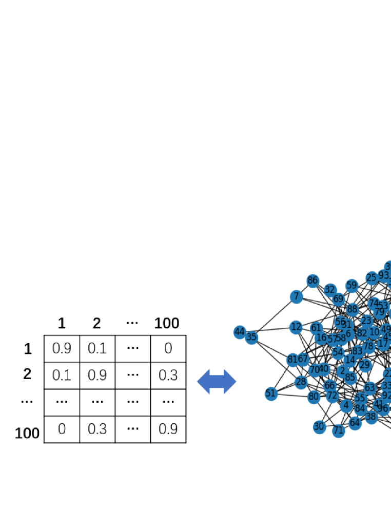
Figure 1: An example of simulate the fixed connection and random contact between $100$ individuals by the random matrix: the matrix and the corresponding network. Individual $2$ has closer connection with individual $100$ than $1$. The recover coefficient for each individuals is $0.9$.

2.2 The Rule of Diseases Spreading

In this section, we introduce the rule where a disease spread on the random matrix.

After the construction of the random matrix characterizing the social connection between a given group of individuals, we set up the following rule to simulate the spreading of the diseases. (1) A vector $x$, named the criterion vector, of size $N\times 1$ is given characterizing the disease infection status of each individual. The $ith$ component of the criterion vector evaluates the exposure to the disease. (2) If the exposure to the disease is below a certain value, the pathogenic threshold, the individual is health. Otherwise, he becomes infected. If the exposure beyond the given value, the lethal threshold, the individual will die. If the exposure return to a value below the pathogenic threshold, he is recovered. The diseases are mainly characterized by the recover coefficient and the pathogenic and lethal thresholds. (3) The spreading of the disease is simulated by considering the random matrix $A$ as the transition probability matrix and the criterion vector $x$ as the vector of state in a Markov process. In a transition probability matrix, the summation of a row is $1$ making the total probability conserved. However, here, the elements of the matrix is not regarded as a probability and the summation of the row of the random matrix is not $1$. Therefore, we name it as the Markov-like process. The spreading is described by the following equation,

$$x_{n+1}=Ax_{n},$$ (2.1)

where $x_{n+1}$ is the criterion vector of next round. For the sake of clarity, we give an example where $10$ individuals are considered, as shown in Fig. (2).

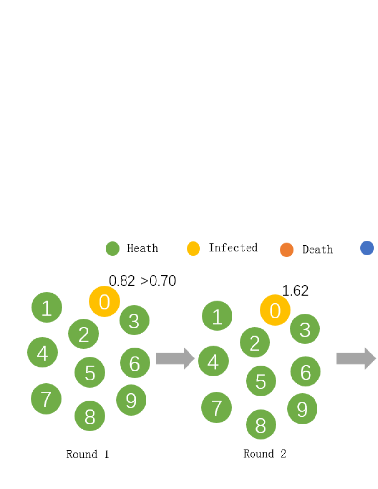
Figure 2: An example illustrating the spreading of the disease. The pathogenic threshold is $0.70$ and the lethal threshold is $3.00$.

To summarize, in this approach, the diseases are characterized by the recover coefficient and the pathogenic and lethal thresholds. And the social connections are described by the random matrix generated under the constraint characterized by the average number of contacts and the average exposure coefficient. By applying the rules, we can simulate the spreading of different diseases under various realistic situations, as show in Fig. (3).

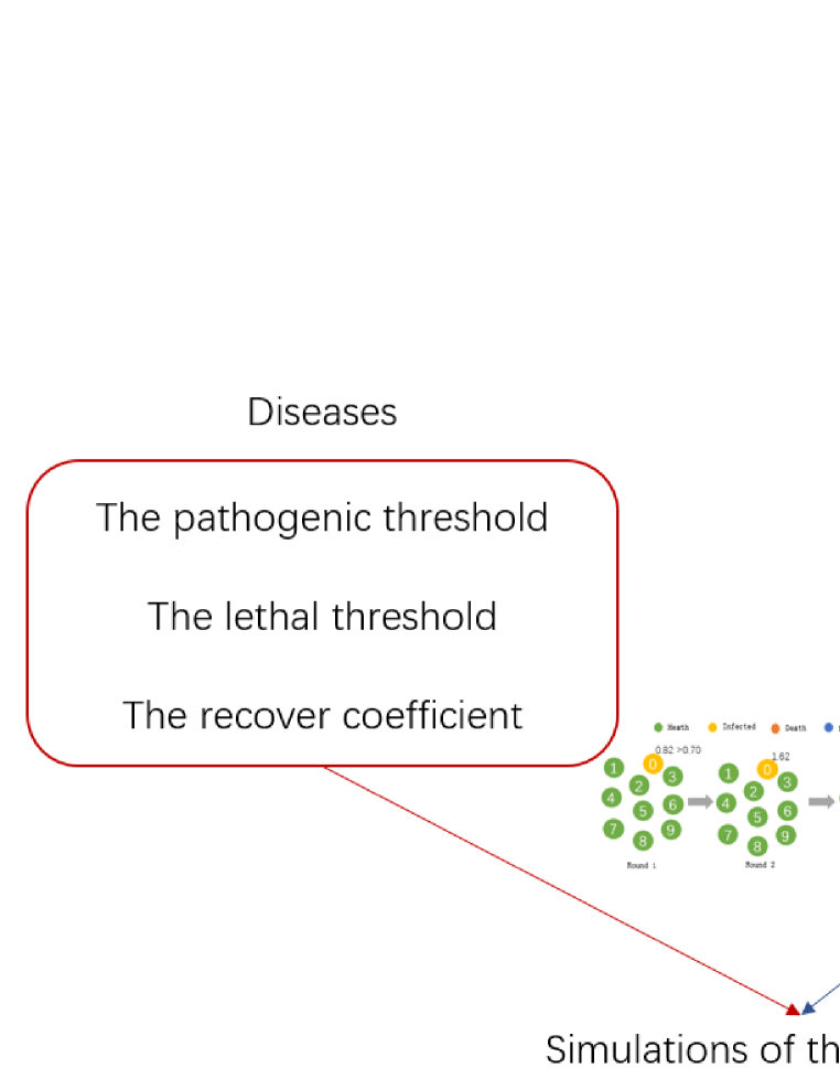
Figure 3: An example illustrating the spreading of the disease. The pathogenic threshold is $0.70$ and the lethal threshold is $3.00$.

3 The Model’s Parameter and Some Discussions

In this section, before conducting various simulations by the proposed models, we give explanations to the model’s parameters since the estimation of model’s parameters is always important. Beside, we report an interesting property of the proposed model and give a simple discussion on the outbreak threshold of the epidemic spreading.

3.1 The Model’s Parameter

Usually, the model’s parameters should be estimated and verified based on the real data first, and then the model could be used to simulate the spreading. In this work, the main aim is to propose a model that can give a large amount of simulations in a given time supporting the searching of the optimal disease control strategy. Therefore, we focus on testing the flexibility of the proposed model to simulate various realistic situations by setting the model’s parameters manually. The estimating of the parameter will be considered in further researches.

In this section, we consider three types of diseases with low, medium, and high pathogenic and lethal thresholds. These three types of diseases represent the general and malignant infectious diseases. Given that the social connections between individuals are described by the random matrix generated under the constraint characterized by the average number of contacts and the average exposure coefficient and the matrix will be altered during the simulation according to different control measures, we set the average number of contacts $4$ and the average exposure coefficient $0.13$. An overview of the setting of model’s parameter is given in Table. (1)

Table 1: The setting of model’s parameter. Av-cont-coe, Av-cont-num, Path-thre, Leth-thre, and Rec-coe stand for the average exposure coefficient, the average number of contacts, the pathogenic threshold, the lethal threshold, and the recover coefficient respectively.

Diseases	Av-exp-coe	Av-cont-num	Path-thre	Leth-thre	Rec-coe
Malignant	$0.13$	$4.0$	$0.4$	$4.0$	$0.9$
Moderate	$0.13$	$4.0$	$0.7$	$6.0$	$0.7$
General	$0.13$	$4.0$	$0.9$	$8.0$	$0.5$

Here is a diagram, Fig. (4), showing the spreading of these three types of diseases. The curve trends and the infected and death populations show the differences.

3.2 An Interesting Property: the Model is Invariant of the Size of the Model

Usually, to simulate the spreading of diseases closer to the realistic situations, one needs to simulate a system with large number of individuals. For example, a small town consists of $100$ thousand populations. In this section, we report an interesting property of the proposed model: the model is invariant of the size. That is, the main indicators of disease transmission, such as the death rate and the infection rate of simulations, remain stable and are invariant of the population sizes, as shown in Table. (2).

To investigate this interesting property, we also repeat the experiments on community networks, a kind of networks describing the social connection of individuals in realistic world. The random matrix describing the community networks can be easily constructed. For example, for the network proposed in this work, the elements of the matrix are sampled from a Gauss distribution under given constraint, see section 2.1. For the community networks, between individuals in a community, the random matrix is generated in the same way, however, between individuals in different communities, only selected individuals have connections, say $5$. Here is the results of another sets of experiments, as shown in Table. (3).

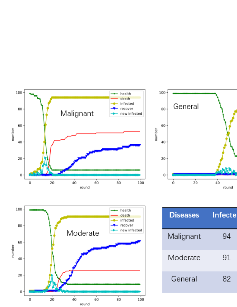
Figure 4: A diagram showing the spreading of these three types of diseases. We consider $100$ individuals with average number of contacts $4$ and the average exposure coefficient $0.13$.

Tables. (2) and (3) shows that the main indicators of disease transmission is invariant of the size of the population. It means that, without loss of generality, the following simulations can be conducted in a model of small number of population, say $100$, which saves computer resources to a desirable extent. Moreover, Fig. (5) shows the difference between simulations of the spreading of diseases on the network proposed in this work and the community networks. Although, the construction of those two random matrices are different, to construct random matrices describing those networks is easy. It shows in Fig. (5) that the spreading on the community network can be divided into different stages while that on the networks provided in this work has only one stage. It is because the spreading of diseases on different communities is not synchronous.

Table 2: The main indicators of disease transmission in different simulations with different population size. The average exposure coefficients is $0.13$, the average number of contacts is $4$, the pathogenic threshold is $0.7$, the lethal threshold is $6.0$, and the recover coefficient is $0.7$.

N	Infection rate	Death rate
$100$	$0.910$	$0.260$
$500$	$0.894$	$0.260$
$1000$	$0.895$	$0.243$
$2000$	$0.900$	$0.249$

Table 3: The main indicators of disease transmission in different simulations on community networks. Con-of-com stands for the number of connections between communities.

N	Con-of-com	Infection rate	Death rate
$100$	$1$	$0.660$	$0.280$
$500$	$1$	$0.664$	$0.286$
$1000$	$1$	$0.672$	$0.314$
$2000$	$1$	$0.665$	$0.297$
$2000$	$2$	$0.699$	$0.305$
$2000$	$5$	$0.686$	$0.301$
$2000$	$10$	$0.747$	$0.309$

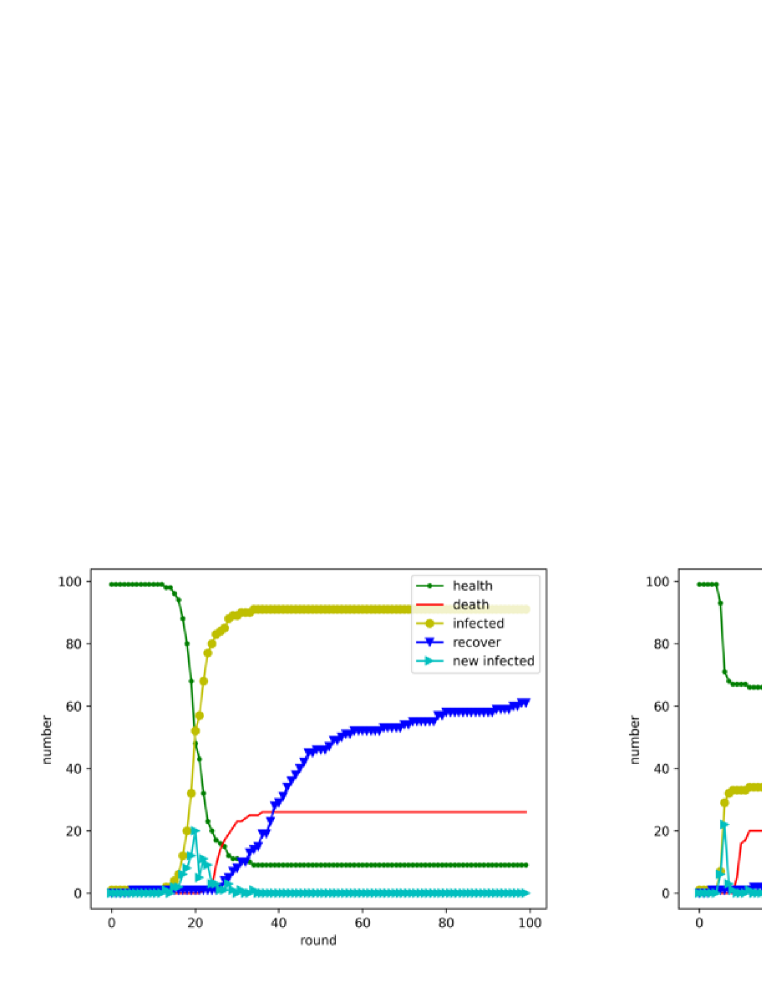
Figure 5: A comparision between the simulations of the spreading of diseases on the network proposed in this work and the community networks.

In the following simulations, we consider $100$ individuals. Here we only report this interesting property and further research on this phenomenon will be carried out in later works.

3.3 A Simple Discussion on Whether the Infectious Disease Will Break Our or Not

In this section, we investigate the outbreak threshold of the epidemic spreading. Instead of a rigorous discussion, we give a simple discussion on whether the infectious disease will outbreaks or not. Further investigation on the equilibrium and nonequilibrium phenomena and thresholds of epidemic spreading will be given in later work.

To explore the outbreak threshold of the epidemic spreading, in this approach, we take the advantages of the proposed method and obtain a large number of simulations where the spreading of different diseases on various situations are considered. Here, the outbreak of the epidemic spreading is defined as over $70\%$ populations are infected. It shows in Fig. (6) that there is a clear boundary between the outbreak and no outbreak cases. For example, the diseases with low pathogenic threshold won’t break out regardless of the average number of contacts of the social network.

Figure 6: A diagram showing the result of simulations where the spreading of different diseases on various situations are considered. The orange triangle represents that the epidemic dose not break out and the blue dot represents breakout. The recover coefficient is $0.7$ and the average exposure rate is $0.13$.

4 The Simulation of the Spreading of Different Diseases under Different Realistic Scenarios

In this section, we simulation of the spreading of different diseases under different realistic scenarios. The diseases are mainly characterized by the pathogenic and lethal thresholds and the realistic scenarios are simulated by the random matrix. For instance, to simulate the spreading of the diseases under the scenario where the control measures of isolating the infected is adopted, the random matrix is altered after each round. The elements corresponding to the infected individuals are all set to $0$.

4.1 Scenarios 1: the Effectiveness of Passive Quarantine

In this section, we consider the effectiveness of passive quarantine. The quarantine can be simply simulated by setting the matrix elements corresponding to the individual $0$ if we find this individual need to be in quarantine. In this simulation only those who go to hospital seeking for a treatment themselves are considered to be in quarantine. Usually, not all infected individuals go to hospital seeking for medical treatment and not all be diagnosed due to wrong diagnosis. Therefore, in this simulation, we set the probability of being diagnosed $0.3$. That is for those who are infected, only $30\%$ will be diagnosed and quarantined. It shows in Fig. (7) and Table. (4) that the quarantine contributes greatly to reduce the infected and death cases in the spreading of the diseases.

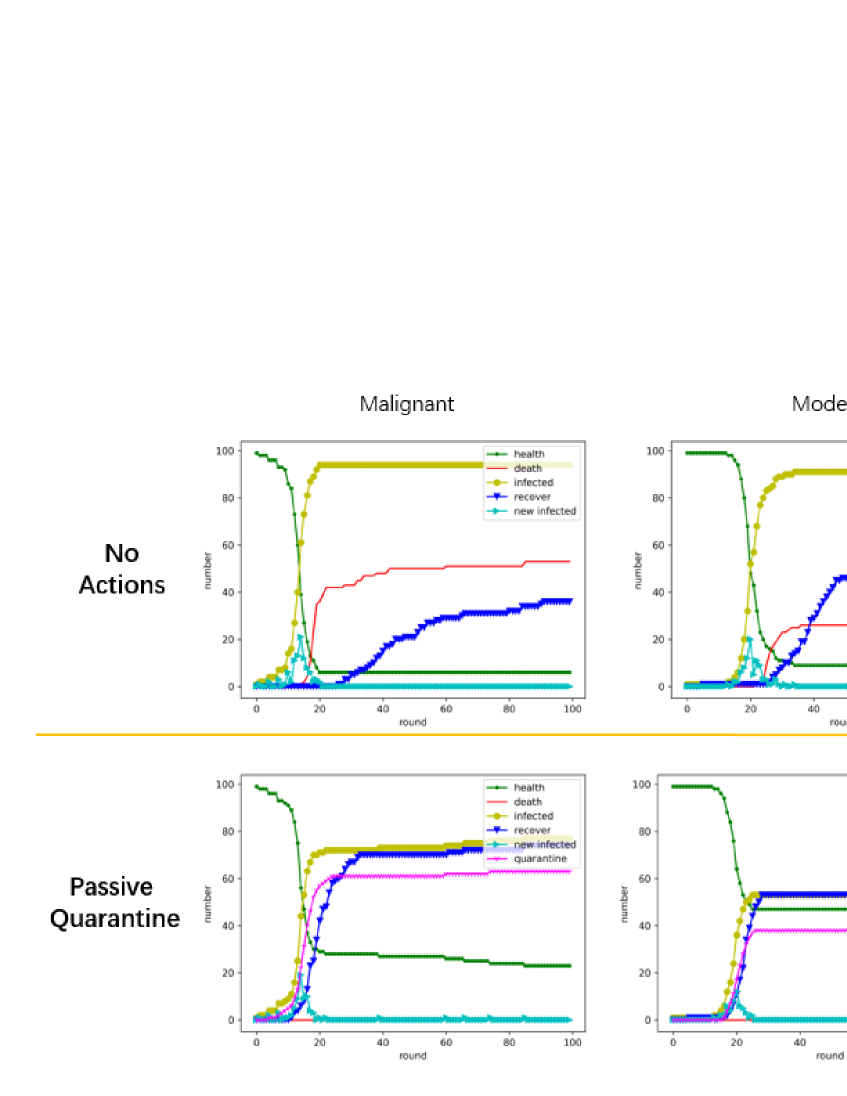
Figure 7: The simulations of spreading under passive quarantine and no actions. The curve trends show the effectiveness of passive quarantine. For example, the infected and death are obviously reduced.

Table 4: The main indicators of spreading under passive quarantine and no actions. The infection rate and the death rate (the ratio between death and all population) show the effectiveness of passive quarantine.

Diseases	Scenarios	Infected	Death
$Malignant$	$Noquarantine$	$94$	$53$
	$Quarantine$	$77$	$0$
$Moderate$	$Noquarantine$	$91$	$26$
	$Quarantine$	$53$	$0$
$General$	$Noquarantine$	$82$	$9$
	$Quarantine$	$20$	$0$

Here are another simulations where the probability of being diagnosed $0.4$, $0.2$, and $0.1$ respectively, as shown in Fig. (8). The simulations suggest that the probability of being diagnosed to be an infected is crucial for the deaths. For example, when the probability is below $0.1$, there are deaths.

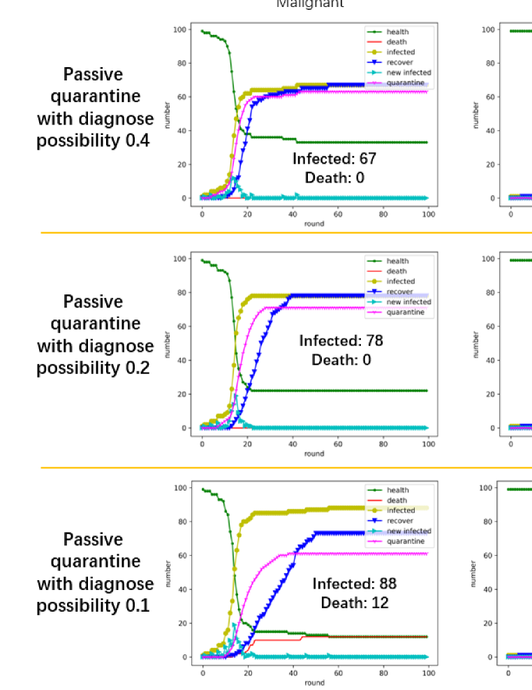
Figure 8: The simulations of spreading under passive quarantine with different diagnose probabilities.

4.2 Scenarios 2: the Effectiveness of Active Quarantine

In this section, we consider the effectiveness of active quarantine. Unlike the passive quarantine, in the active quarantine, we conduct a disease detection for all individuals and those found to be infected are in quarantine. The active quarantine considers those who don’t go to hospital for treatment themselves. Given that the method we use for disease detection is imperfect, that is, the method can’t find all infected individuals. We simulate the cases where the detection recall is $99\%$, $90\%$, and $80\%$ respectively. In realistic life, conducting an overall disease detection costs considerable human and financial costs, therefore, in the simulation, the overall disease detection is conducted every $5$ and $10$ rounds. Figs. (9) and (10) show the effectiveness of active quarantine. The simulations of proposed model show that, the overall disease detection helps little with the control of spreading of the diseases. Increasing the frequency and accuracy of the overall disease detection contributs little to the control of spreading of the diseases too.

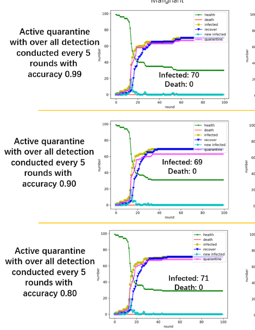
Figure 9: The simulations of spreading under active quarantine with different overall disease detection accuracies. The overall disease detection frequency is every $5$ round.

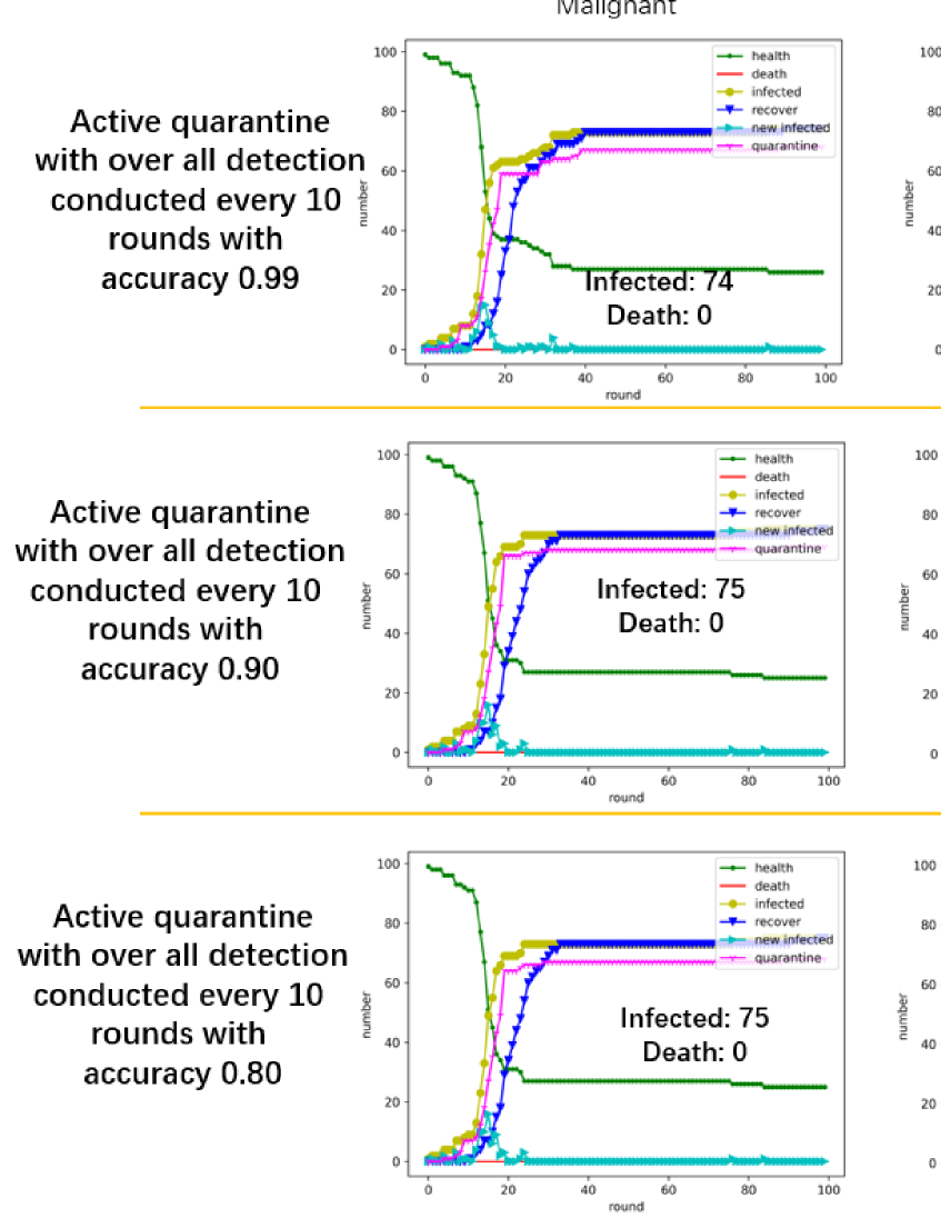
Figure 10: The simulations of spreading under active quarantine with different overall disease detection accuracies. The overall disease detection frequency is every $10$ round.

4.3 Scenarios 3: the Effectiveness of the Green Code

In this section, we consider the effectiveness of the green code, a measure used in China to control the COVID-19. In this control measure, not only those who are diagnosed are quarantined but also those who have direct contact with the infected, namely close contacts, are quarantined too. In this simulations, those who go to hospital seeking for a medical treatment themselves are possibly be diagnosed as infected. The result of simulations are shown in Figs. (11) and (12). It shows that the green code measure contributes to the control of the spreading of the diseases obviously. Especially from the curve trends in Fig. (12), the infected population is reduced obviously.

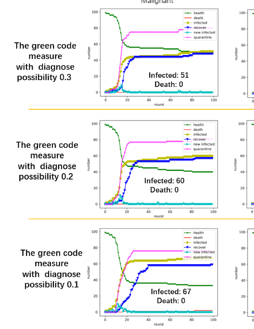
Figure 11: The simulations of spreading under the green code measure with different diagnose probabilities.

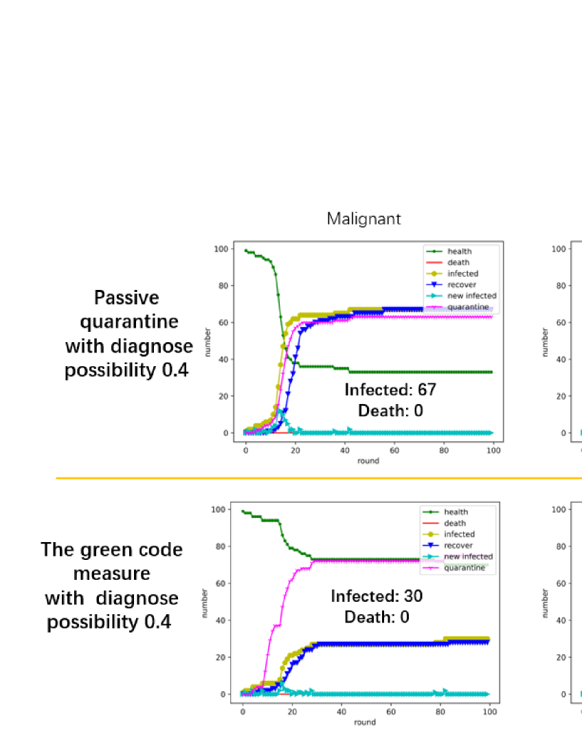
Figure 12: The simulations of spreading under the passive quarantine with and without green code measure.

4.4 Scenarios 4: the Effectiveness of the Green Code and Overall Detection

In this section, we consider the effectiveness of the green code and overall detection. That is, the overall detection is conducted to find the infected population such as those who never go to hospital. Moreover, the infected and the close contacts are quarantined.

The result of simulations are shown in Fig. (13). It shows that the green code measure and overall detection together contribute to the control of the spreading of the diseases to some degree. For the malignant infectious disease the control measure is with higher effectiveness. The simulation suggests that to effectively control the spreading of the disease, to find the infected and their close contacts and make them quarantined are the keys.

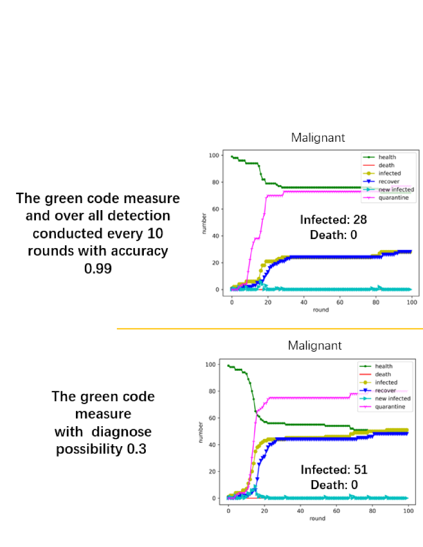
Figure 13: The simulations of spreading under the green code measure with and without overall detection.

4.5 Scenarios 5: Asymptomatic Carriers

In this section, we consider the asymptomatic carriers. The asymptomatic carriers are individuals who are infected and are contagious but have no uncomfortable signs and symptoms. Usually, the asymptomatic carriers are hard to be found. In the following simulations, we consider the spreading of diseases with asymptomatic carriers under the most strict control measures, the green code and overall detection. Here, we make the assumption that the asymptomatic carriers can not be found even in the overall detection.

The result of simulations are shown in Fig. (14). It shows that the asymptomatic carriers are the main group to break down the strict control measure, the green code and overall detection. Especially when there are over $10\%$ of the populations are asymptomatic carriers, there are deaths.

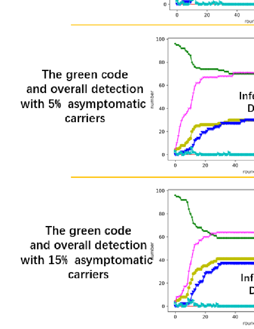
Figure 14: The simulations of spreading with asymptomatic carriers under the green code and overall detection.

4.6 Scenarios 6: Vaccination

In this section, we consider the spreading of diseases with vaccination. The vaccination is a useful method to control the spreading of diseases. In this simulation, we make the assumption that the vaccination will increase the resistance of the pathogens. That is the pathogenic and lethal thresholds stay the same, but the recover coefficient will the lowered. The lower the recover coefficient the quicker the infected will recover. Here, after vaccination, the recover coefficient multiplies $0.7$.

The result of simulations are shown in Fig. (15). It shows that the vaccination can effectively control the spreading of diseases, especially for the general infectious diseases. However, to avoid deaths, only vaccination is not enough. That is, we need control measures such as the quarantine and green code.

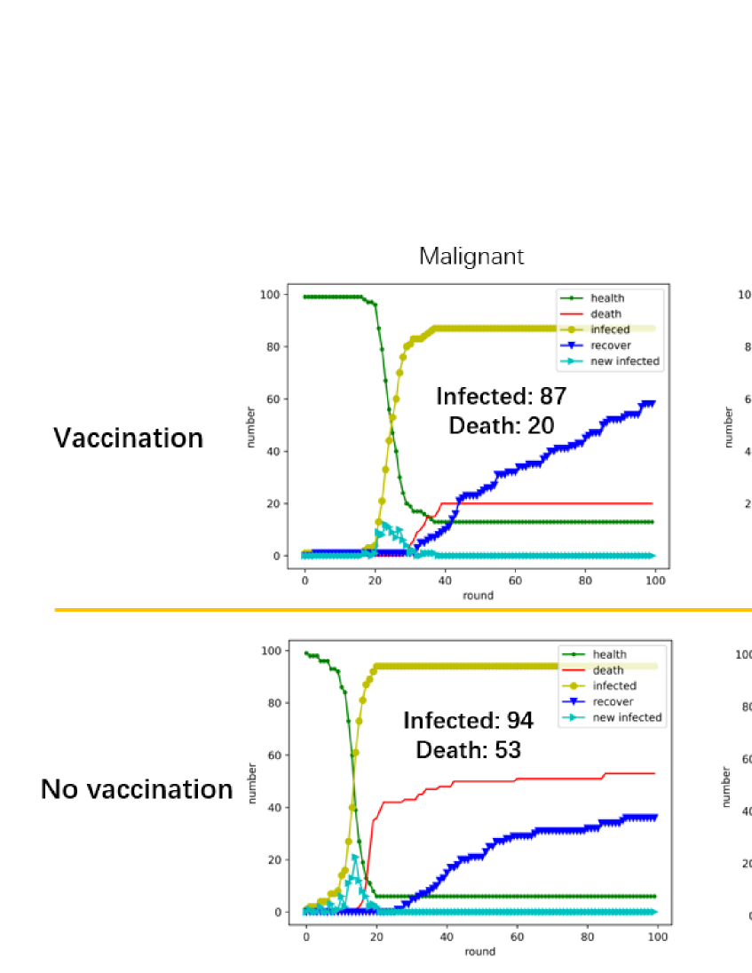
Figure 15: The simulations of spreading with and without vaccination.

4.7 Scenarios 7: Mask Wears

In this section, we consider diseases spread by air, and to wear a mask can efficiently prevent the spreading. Here, we consider two kinds of mask, one is medical mask and the other is the general mask. In this simulation, the medical mask can reduce the exposure coefficient by multiplying $0.9$ and the general mask $0.95$. Without loss of generality, we make assumption that all individuals wear masks.

The result of simulations are shown in Fig. (16). It shows that wearing a mask can control the spreading of diseases, especially for the general infectious diseases the medical mask reduces the deaths to $0$.

Figure 16: The simulations of spreading with medical and general masks.

5 Conclusions and Discussions

Establishing a model that can simulate the spread of infectious diseases is the key to studying the law of infectious disease transmission and predicting the trend of transmission, and it is of great significance to control the spread of infectious diseases. To find the optimal control strategy, we need a large number of simulations to support the searching process. Therefore, one needs the model that can at one hand simulate the spreading of diseases under realistic conditions and at the other hand quickly return the result of the simulations. In the realistic social network, on the one hand, the random contact, including the contact with strangers at public places, becomes more and more important access for the spreading of diseases. One the other hand, the individuals are different form one to the other, and the individual differences will effect the spreading of diseases. For example, the asymptomatic carriers will cause a wider spread of the disease.

In this work, a model that can simulate the spreading of diseases under realistic situations with random contact is proposed. Unlike the conventional approaches, such as the differential equation based compartment models, the cellular automata and the complex network based models, the social connections, in this approach, are described by using the random matrix which is generated under given constraint, the average contact population and the average exposure coefficient. The spreading of the disease is simulated by using the Markov-like process, where the random matrix is considered as a probability transition matrix with the exposure coefficient (the elements of the random matrix) the transition probability. The diseases are characterized by the recover coefficient and the pathogenic and lethal thresholds. Instead of estimating the model’s parameters according to the real data, we firstly manually choose the parameters, in order to simulate the spreading of diseases under various realistic scenarios. We report an interesting property of the proposed method: the major indicators such as the infection and death rates are almost invariant of the size of the model.

A set of experiments show that the proposed model can efficiently simulate the spreading of various diseases under various realistic situations. Therefore, the proposed model can give a large number of simulations supporting the searching of optimal diseases control strategy in the following researches. In the next research, the reinforcement learning method, a method that is good at finding the optimal strategy, will be introduced. Together with the proposed model, we give a further investigation to the optimal control strategy of the infectious diseases.

6 Acknowledgments

We are very indebted to Prof. Wu-Sheng Dai for his enlightenment and encouragement. We are very indebted to Prof. Guan-Wen Fang for his encouragement. This work is supported by National Natural Science Funds of China (Grant No. 62106033), Yunnan Youth Basic Research Projects (202001AU070020), and Doctoral Programs of Dali University (KYBS201910). YuanYuan Wang acknowledges the support from Yunnan Fundamental Research Projects (grant NO. 2019FD099)

7 Conflict of interest statement

We declare that we have no financial and personal relationships with other people or organizations that can inappropriately influence our work, there is no professional or other personal interest of any nature or kind in any product, service and/or company that could be construed as influencing the position presented in, or the review of, the present manuscript.

References

- [1] A. Bhatele, J. S. Yeom, N. Jain, C. J. Kuhlman, and M. V. Marathe, Massively parallel simulations of spread of infectious diseases over realistic social networks, in 2017 17th IEEE/ACM International Symposium on Cluster, Cloud and Grid Computing (CCGRID), 2017.
- [2] S. N. DeWitte and J. W. Wood, Selectivity of black death mortality with respect to preexisting health, Proceedings of the National Academy of Sciences 105 (2008), no. 5 1436–1441.
- [3] N. Fernandes, Economic effects of coronavirus outbreak (covid-19) on the world economy, .
- [4] K. Dietz and J. Heesterbeek, Daniel bernoulli’s epidemiological model revisited, Mathematical Biosciences 180 (2002), no. 1-2 1–21.
- [5] W. H. Hamer, Epidemic disease in england-the evidence of variability and of persistency of type, Lancet 167 (1906), no. 4306 655–662.
- [6] R. Ross, The prevention of malaria. John Murray, 1911.
- [7] O. Diekmann, J. A. P. Heesterbeek, and J. A. Metz, The legacy of kermack and mckendrick, Publications of the Newton Institute 5 (1995) 95–115.
- [8] D. Breda, O. Diekmann, W. De Graaf, A. Pugliese, and R. Vermiglio, On the formulation of epidemic models (an appraisal of kermack and mckendrick), Journal of biological dynamics 6 (2012), no. sup2 103–117.
- [9] Y. Maki and H. Hirose, Infectious disease spread analysis using stochastic differential equations for sir model, in 2013 4th International Conference on Intelligent Systems, Modelling and Simulation, pp. 152–156, IEEE, 2013.
- [10] W. E. Eyaran, S. Osman, and M. Wainaina, Modelling and analysis of seir with delay differential equation, Global Journal of Pure and Applied Mathematics 15 (2019), no. 4 365–382.
- [11] R. H. Chisholm, P. T. Campbell, Y. Wu, S. Y. Tong, J. McVernon, and N. Geard, Implications of asymptomatic carriers for infectious disease transmission and control, Royal Society open science 5 (2018), no. 2 172341.
- [12] A. Gray, D. Greenhalgh, L. Hu, X. Mao, and J. Pan, A stochastic differential equation sis epidemic model, SIAM Journal on Applied Mathematics 71 (2011), no. 3 876–902.
- [13] L. J. Allen, A primer on stochastic epidemic models: Formulation, numerical simulation, and analysis, Infectious Disease Modelling 2 (2017), no. 2 128–142.
- [14] M. R. Islam et al., Mathematical modeling of infectious diseases using ordinary and fractional differential equations. PhD thesis, 2020.
- [15] G. Huang, Y. Takeuchi, and W. Ma, Lyapunov functionals for delay differential equations model of viral infections, SIAM Journal on Applied Mathematics 70 (2010), no. 7 2693–2708.
- [16] S. Greenhalgh and C. Rozins, A generalized differential equation compartmental model of infectious disease transmission, Infectious Disease Modelling 6 (2021) 1073–1091.
- [17] V. A. Meszaros, M. D. Miller-Dickson, F. Baffour-Awuah, S. Almagro-Moreno, and C. B. Ogbunugafor, Direct transmission via households informs models of disease and intervention dynamics in cholera, PLoS One 15 (2020), no. 3 e0229837.
- [18] Z. Mukandavire and J. G. Morris Jr, Modeling the epidemiology of cholera to prevent disease transmission in developing countries, Microbiology spectrum 3 (2015), no. 3 3–3.
- [19] M. A. Acevedo, O. Prosper, K. Lopiano, N. Ruktanonchai, T. T. Caughlin, M. Martcheva, C. W. Osenberg, and D. L. Smith, Spatial heterogeneity, host movement and mosquito-borne disease transmission, PloS one 10 (2015), no. 6 e0127552.
- [20] B. Zheng, M. Tang, and J. Yu, Modeling wolbachia spread in mosquitoes through delay differential equations, SIAM Journal on Applied Mathematics 74 (2014), no. 3 743–770.
- [21] A. G. Buchwald, J. Adams, D. M. Bortz, and E. J. Carlton, Infectious disease transmission models to predict, evaluate, and improve understanding of covid-19 trajectory and interventions, Annals of the American Thoracic Society 17 (2020), no. 10 1204–1206.
- [22] S. S. Nadim and J. Chattopadhyay, Occurrence of backward bifurcation and prediction of disease transmission with imperfect lockdown: A case study on covid-19, Chaos, Solitons & Fractals 140 (2020) 110163.
- [23] L. López, G. Burguerner, and L. Giovanini, Addressing population heterogeneity and distribution in epidemics models using a cellular automata approach, BMC research notes 7 (2014), no. 1 1–11.
- [24] P. Jithesh, A model based on cellular automata for investigating the impact of lockdown, migration and vaccination on covid-19 dynamics, Computer methods and programs in biomedicine 211 (2021) 106402.
- [25] J. Dai, C. Zhai, J. Ai, J. Ma, J. Wang, and W. Sun, Modeling the spread of epidemics based on cellular automata, Processes 9 (2020), no. 1 55.
- [26] A. Holko, M. Medrek, Z. Pastuszak, and K. Phusavat, Epidemiological modeling with a population density map-based cellular automata simulation system, Expert Systems with Applications 48 (2016) 1–8.
- [27] S. Ghosh and S. Bhattacharya, A data-driven understanding of covid-19 dynamics using sequential genetic algorithm based probabilistic cellular automata, Applied Soft Computing 96 (2020) 106692.
- [28] M. Precharattana, Stochastic modeling for dynamics of hiv-1 infection using cellular automata: A review, Journal of bioinformatics and computational biology 14 (2016), no. 01 1630001.
- [29] S. Bin, G. Sun, and C.-C. Chen, Spread of infectious disease modeling and analysis of different factors on spread of infectious disease based on cellular automata, International journal of environmental research and public health 16 (2019), no. 23 4683.
- [30] M. Draief, Epidemic processes on complex networks, Physica A: Statistical Mechanics and its Applications 363 (2006), no. 1 120–131.
- [31] R. Pastor-Satorras, C. Castellano, P. Van Mieghem, and A. Vespignani, Epidemic processes in complex networks, Reviews of modern physics 87 (2015), no. 3 925.
- [32] R. Pastor-Satorras and A. Vespignani, Epidemic spreading in scale-free networks, Physical review letters 86 (2001), no. 14 3200.
- [33] Y. Moreno, J. B. Gómez, and A. F. Pacheco, Epidemic incidence in correlated complex networks, Physical Review E 68 (2003), no. 3 035103.
- [34] C. Castellano and R. Pastor-Satorras, Thresholds for epidemic spreading in networks, Physical review letters 105 (2010), no. 21 218701.
- [35] S. Xu, W. Lu, and L. Xu, Push-and pull-based epidemic spreading in networks: Thresholds and deeper insights, ACM Transactions on Autonomous and Adaptive Systems (TAAS) 7 (2012), no. 3 1–26.
- [36] M. Boguná and R. Pastor-Satorras, Epidemic spreading in correlated complex networks, Physical Review E 66 (2002), no. 4 047104.
- [37] Q. Wu and X. Fu, Immunization and epidemic threshold of an sis model in complex networks, Physica A: Statistical Mechanics and its Applications 444 (2016) 576–581.
- [38] X. Zhang, J. Wu, P. Zhao, X. Su, and D. Choi, Epidemic spreading on a complex network with partial immunization, Soft Computing 22 (2018), no. 14 4525–4533.
- [39] A. Edelman and N. R. Rao, Random matrix theory, Acta Numerica 14 (2005), no. 1 233–297.
- [40] Thomas, Guhr, , , Axel, Müller–Groeling, , , Hans, A., and Weidenmüller, Random-matrix theories in quantum physics: common concepts, Physics Reports 299 (1998), no. 4-6 189–425.
- [41] A. M. Tulino, S. Verdú, et al., Random matrix theory and wireless communications, Foundations and Trends® in Communications and Information Theory 1 (2004), no. 1 1–182.