Selecting and scheduling an optimal subset of road network upgrades

Abstract

We consider the problem of choosing a subset of proposed road network upgrades to implement within a fixed budget in order to optimize the benefit in terms of vehicle hours travelled (VHT), and show how to render the solution of this problem more tractable by reducing the number of traffic assignment problems that must be solved. This technique is extended to develop a heuristic algorithm for finding a schedule of road upgrades over a planning period that maximizes the net present value of the resulting VHT reductions.

Keywords— traffic assignment problem, constrained optimization, network modelling, road upgrade scheduling

1 Introduction

Consider the problem of deciding, amongst a set of proposed upgrades to an urban road network, which subset to implement given a fixed budget that constrains the selection. In order to make this selection in a rational way, we must associate some benefit with each possible subset. One of the most obvious such benefits is simply the reduction in total travel time across the system, which we can measure in vehicle hours travelled (VHT) per day, due to the upgrade.

In order to compute the change in VHT for a particular upgrade, we must solve the traffic assignment problem (TAP). This is an important problem in transportation research and in the practical application of modelling to transportation planning. This problem is to predict the route choice of users of a road network given sets of origins and destinations for trips. Once these routes have been computed, the level of congestion on each road is determined, and proposed changes to a road network can be compared by their effects on the final congested network.

The importance of the traffic assignment problem has led to it being an active area of research for many years, and a comprehensive overview can be found in Patriksson (1994). Although there are many approaches and variations to traffic modelling, we restrict ourselves to the “traditional” static assignment at user equilibrium (UE). In this model, we make the assumption that each traveller chooses the route that minimizes his or her own travel time, given the current traffic flows on the road network. These travel times are a function of the traffic flows resulting from the routes chosen by all the travellers, and the user equilibrium is achieved when no traveller can improve his or her travel time by unilaterally choosing a different route. It is important to note that adding capacity (such as a new road) to a road network does not necessarily reduce the total VHT, since the UE, which is optimal for each traveller, is not necessarily the optimum for the system as a whole. Such a situation, when adding capacity increases the system-wide travel time, is known as Braess’s paradox.

This UE model has been formulated as a convex quadratic optimization problem (Beckmann et al., 1956; Dafermos and Sparrow, 1969), which can be solved efficiently by the Frank-Wolfe algorithm (Frank and Wolfe, 1956; LeBlanc et al., 1975). Although more sophisticated and faster converging algorithms have been demonstrated, such as path-based assignment (Jayakrishnan et al., 1994; Dial, 2006), origin-based assignment (Bar-Gera, 2002), and LUCE (Gentile, 2009), the simplicity of the Frank-Wolfe algorithm, its small memory requirements, and its capacity for simple parallelization mean that it is still competitive on efficiency in practice, and widely used, for example in commercial products such as PTV A.G.’s VISUM (PTV AG, ) (which now also implements the LUCE algorithm), Citilabs’s Cube Voyager (Citilabs, ), and Caliper’s TransCAD (Caliper, ; Slavin et al., 2006).

In order to solve our constrained optimization problem (maximize reduction in VHT by selecting a subset of possible upgrades within a fixed budget), we must at least compute the reduction in VHT due to each individual upgrade in isolation. However, this might not be enough, since the change in VHT due to two or more upgrades made to the network need not necessarily simply be the sum of the changes individually. To solve the problem exactly, we would in principle have to compute the VHT for every member of the power set of the set of possible upgrades, an exponentially large number of traffic assignment problems that is clearly infeasible in practice, especially given that each TAP takes several hours to solve to acceptable accuracy for a realistic city road network. By considering only pairwise interactions, on the assumption that interactions of a higher order can be ignored, this can be reduced to a quadratic number of TAPs to solve, which for a large number of possible upgrades is still most likely impractical. In this paper we show how to approximate an optimal solution within a practical time by solving a model which incorporates pairwise interactions between upgrades only when two individual road upgrades are estimated to have a pairwise VHT change value that is significantly different from the sum of their individual contributions. That is, we need only solve the TAP for each individual upgrade, and for a small number of pairs of upgrades. Further, we present a model, and a heuristic algorithm to approximate an optimal solution, for the problem of scheduling the upgrades in a planning period in order to maximize the net present value of the VHT reductions.

Recently, Wu et al. (2011) presented a formulation and solution of the “project selection problem” in the context of build-operate-transfer developments of road networks. Their formulation involves finding projects that both have a societal benefit (VHT reduction) and are also attractive to private developers bidding for the development, a function of the tolls they are able to charge. Therefore, their formulation involves finding the optimal capacity increases and tolls for projects to be contracted to private firms under the build-operate-transfer scheme. In contrast, the project selection problem we solve here operates under the simpler scheme of selecting from a set of candidate highway upgrades those with the maximal benefit within a fixed budget. Our focus is on reducing the number of TAPs to solve without unduly reducing the accuracy of the resulting VHT reduction estimates. In addition, we extend the problem to project scheduling, where we show a method to select the projects to build in each year of a planning period, given a budget for each year, in order to maximize the net present value of the societal benefit (reductions in VHT).

2 Methods

In order to find the optimal subset of a set of road upgrades within a fixed budget, we need to first solve the TAP on the existing network to obtain a VHT value for the current (before upgrade(s)) situation. From then on we consider changes (hopefully reductions) in the VHT from this base value for each upgrade. Solving the TAP requires the usual inputs to this process: the road network, with parameters specifying the relationship between volume (flow) and travel time (cost) on each link, and the Origin-Destination (O-D) demand matrix specifying trips on the network. The output of this process is then the volume and latency (cost) on each link at UE, and global statistics such as VHT, which is the sum over all links of the product of the volume and cost on the link.

The outline of the procedure to find the optimal upgrade subset is then:

1. For each individual upgrade, compute VHT by solving the traffic assignment problem on the network modified by that upgrade.

2. Use the pairwise interaction model (Section 2.3) to estimate which pairs of upgrades will have a significant interaction, meaning that their combined effect is significantly different from simply additive.

3. Run traffic assignment on each such pair of upgrades to compute the VHT for these pairs of upgrades.

4. Solve the upgrade subset model (Section 2.2) with the individual and required pairwise upgrade VHT change values to find the optimum subset of upgrades within the specified budget.

2.1 Solving the traffic assignment problem

As mentioned in Section 1, the traffic assignment problem is a well-studied problem. Here we give a brief summary of the user equilibrium in the static traffic assignment problem, and its solution by the Frank-Wolfe method. Details can be found in, for example, Sheffi (1985); Patriksson (1994); Florian and Hearn (1995).

We are given the road network as a graph $G=(\mathcal{N},\mathcal{A})$ where $\mathcal{N}$ is the set of nodes and $\mathcal{A}$ is the set of arcs (links representing road segments). Each arc $a\in\mathcal{A}$ has associated with it a capacity (the maximum number of vehicles that can travel on it per unit time) $Q^{\max}_{a}$ and a free travel time $t_{a}$, the time required to traverse it at the maximum allowed speed. It is assumed that this travel time depends only on the current flow on the arc $f_{a}$ (the number of vehicles using that link), according to a latency function which is continuous and non-decreasing (higher flow means longer latency). The BPR (Bureau of Public Roads) function is usually used for this purpose:

$$l_{a}(f_{a})=t_{a}\left(1+\alpha\left(\frac{f_{a}}{Q^{\max}_{a}}\right)^{\beta}\right)$$ (1)

where $\alpha$ and $\beta$ are parameters, for example $\alpha=0.15$ and $\beta=4.0$.

In addition, we are given a set of origin nodes $\mathcal{O}\subseteq\mathcal{N}$ and destination nodes $\mathcal{D}\subseteq\mathcal{N}$ and an O-D demand matrix $Q_{|\mathcal{O}|\times|\mathcal{D}|}$, such that $(q_{rs})$ gives the number of vehicles from origin $r\in\mathcal{O}$ to destination $s\in\mathcal{D}$ in a given time period. These origin and destination nodes are typically the centroids of zones used in determining trip rates.

The traffic assignment which we are to find is the current state of the traffic network given by the pair $(f,l)$ where $f\in\mathbb{R}^{|\mathcal{A}|}$ is the flow (the volume of cars on each link) and $l\in\mathbb{R}^{|\mathcal{A}|}$ is the travel time (the latency on each link), where $l$ is a function of $f$ (Equation 1). We denote the flow on path $k$ connecting an O-D pair $(r,s)\in\mathcal{O}\times\mathcal{D}$ by $h_{rs}^{k}$, where $k$ is in $\mathbb{P}_{rs}$, the set of paths between origin $r$ and destination $s$.

The user equilibrium is then obtained by solving the convex optimization problem:

$$\min\sum_{a\in\mathcal{A}}\int_{0}^{f_{a}}l_{a}(x)dx$$ (2)

subject to

$$\sum_{k\in\mathbb{P}_{rs}}h_{rs}^{k}=q_{rs} \forall(r,s)\in\mathcal{O}\times\mathcal{D}$$ (3)

$$h_{rs}^{k}\geq 0 \forall k\in\mathbb{P}_{rs},\forall(r,s)\in\mathcal{O}\times\mathcal{D}$$ (4)

$$f_{a}=\sum_{(r,s)\in\mathcal{O}\times\mathcal{D}}\sum_{k\in\mathbb{P}_{rs}}h_{rs}^{k}\delta_{a,k}^{rs} \forall a\in\mathbb{A}$$ (5)

where $\delta_{a,k}^{rs}$ is the indicator variable

$$\delta_{a,k}^{rs}=\left\{\begin{array}[]{lr}1,&\mbox{if link }a\mbox{ is on path }k\mbox{ between O-D pair }(r,s)\\ 0,&\mbox{otherwise}\\ \end{array}\right.$$ (7)

As mentioned in Section 1, this quadratic program is often solved with the Frank-Wolfe algorithm (Frank and Wolfe, 1956) (also known as the convex combinations method). Applied to the UE problem (Equations 2–7), this amounts to iteratively solving a set of shortest-path problems (the “all-or-nothing assignment” of traffic flows) to find search directions followed by a linear program to find search step size, terminating when a convergence criterion is satisfied.

Many termination criteria are possible, but probably the most commonly used is the relative gap (Rose et al., 1988; Slavin et al., 2006). This is the ratio of the difference between the cost of the current solution and the cost of the “all-or-nothing assignment” solution (i.e. the shortest paths that were used to find the search direction) to the cost of the current solution:

$$\frac{\sum f\cdot l(f)-\sum f_{\mbox{aon}}\cdot l(f)}{\sum f\cdot l(f)}$$ (8)

where $f_{\mbox{aon}}$ is the “all-or-nothing” solution. Relative gaps on the order of $10^{-5}$ (or smaller) are usually considered to indicate a very good solution.

Since the shortest path computation is responsible for more than 90% of the CPU time in practical applications (Patriksson, 1994, p. 100), an algorithm that solves this problem for road networks efficiently in practice is important. Although Dijkstra’s algorithm (Dijkstra, 1959) with an appropriate priority queue implementation such as a Fibonacci heap (Fredman and Tarjan, 1987) is among the algorithms with asymptotically smallest time complexity for the single-source shortest path algorithm for general graphs with non-negative edge weights, in practice on large-scale road networks, label-correcting algorithms run faster (Zhan and Noon, 1998; Klunder and Post, 2006). In contrast to the label-setting algorithms, such as Dijkstra’s, which determine exactly the shortest path for one node at each iteration, the label-correcting algorithms do not determine shortest paths for any node until the end of the algorithm. That is, the so-called pivot node (the node whose shortest path is being updated) can be entered into the processing queue multiple times. Each time it is dequeued its label value is an estimate (actually an upper bound) on the cost of the shortest path to that node from the source, and only at termination (when the queue is empty because no smaller labels are found) are the labels exact values for the shortest path costs.

The simplest label-correcting algorithm is the Bellman-Ford algorithm (Bellman, 1957; Ford and Fulkerson, 1965), however in practice on large-scale road networks, better performance can be achieved with other algorithms (Klunder and Post, 2006) such as the d’Esopo-Pape algorithm (Pape, 1974), and the Small Label First (SLF) (Bertsekas, 1993) algorithm, especially with the Large Label Last (LLL) (Bertsekas et al., 1996) modification. The d’Esopo-Pape algorithm always removes nodes from the top of the queue, and enqueues nodes at the bottom of the queue if they have never been in the queue before, otherwise at the top of the queue. The SLF algorithm is, instead of enqueuing according to whether previously in queue or not, whenever a node is enqueued, its label (current distance) is compared with that at the top of the queue, and if its label is smaller than that at the top, it is put at the top, otherwise at the bottom of the queue. In the LLL modification of the algorithm, at each iteration, when the node at the top of the queue has a larger label than the average label of nodes in the queue, this (top) node is not removed as the current node but instead put at bottom of queue (and we keep doing this until a node with smaller than average label is found). Klunder and Post (2006) show that the d’Esopo-Pape and SLF algorithms with the LLL modification are faster in practice on large-scale road networks than Dijkstra’s algorithm and the Bellman-Ford algorithm.

2.1.1 Implementation

We implemented a Frank-Wolfe solution of the above traffic assignment problem in the C programming language, using the d’Esopo-Pape algorithm with the LLL modification (we found that on our test network (see Section 3) the d’Esopo-Pape algorithm with the LLL modification was faster than the SLF algorithm with the LLL modification) to solve the shortest path problems. Since the Frank-Wolfe algorithm involves solving the shortest path problem for each O-D node pair at each iteration, and each of these computations is independent, we can execute these computations in parallel, and our implementation does so using POSIX threads (pthreads) to take advantage of multicore processors. The resulting updates of the link volumes vector are also executed in parallel, in a lock-free manner using processor atomic instructions to ensure correctness.

We require the solution of the TAP not only for the original road network, but also for the road network modified by the set of potential upgrades, some pairs of potential upgrades, and, for evaluation purposes in our test cases, all pairs of upgrades and all subsets of the upgrade set. Hence our implementation takes as an additional input a file containing the description of the upgrade set, with options to run with each modification, pairwise modifications, or all subsets of modifications. Since these different modified road networks are processed independently, they can be run in parallel and the Message Passing Interface (MPI) is used to distribute the computations across different processors and nodes where available.

Source code for our implementation is available from https://github.com/stivalaa/traffic_assignment.

2.2 A model to determine the optimal subset of upgrades

If, for $N$ upgrades, we know the VHT change for each individual upgrade, $v_{i}$, and the VHT change for each pair of upgrades $\Delta\mbox{VHT}_{ij}$, giving us the difference between the pairwise change and the sum of individual changes, $d_{ij}=\Delta\mbox{VHT}_{ij}-(v_{i}+v_{j})$ then the optimal subset can be found by the following constrained optimization problem:

$$\max\left(\sum_{1\leq i<j\leq N}y_{i}y_{j}d_{ij}m+\sum_{1\leq i\leq N}y_{i}(v_{i}m-c_{i})\right)$$ (9)

subject to

$$\sum_{1\leq i\leq N}y_{i}c_{i}\leq B$$ (10)

where $c_{i}$ is the cost of upgrade $i$ and $B$ is the total budget and $y_{i}\in\{0,1\}$ is an indicator variable such that $y_{i}=1$ if upgrade $i$ is in the selected subset.

In order to convert a VHT reduction $v$ to a monetary amount, the factor $m$ is required that gives a dollar value to each vehicle hour travelled. This may be some estimate of the average value of each traveller’s time, and will likely be some value on the order of $10, for example. In addition, since our traffic models operate on daily VHT values, we must multiply by 365 to convert to annual values, so, combining these considerations we might use for example $m=3650$. We use this value of $m$ to compute the results presented in Section 3. In a more detailed analysis we might have separate models for AM and PM peaks on weekdays and for weekends, and hence the appropriate different factors will be used to convert these to annual monetary benefits.

The objective function (Equation 9) is quadratic because as well as the benefit for each individual upgrade we account for the possibly different benefit for each pair of upgrades in the case both in the pair are in the subset considered.

Note the VHT change $v_{i}$ for a change $i$ is $\mbox{VHT}_{0}-\mbox{VHT}_{i}$ where $\mbox{VHT}_{0}$ is the baseline VHT value, that is, the VHT for the existing road network with no upgrades. Therefore a positive value of $v_{i}$ denotes an improvement (i.e. reduction) in the VHT value relative to the baseline due to change $i$.

This model can be easily expressed in the MiniZinc (Nethercote et al., 2007) modelling language and solved with the ECLⁱPS^e interval arithmetic constraint solver (Schimpf and Shen, 2010; Brisset et al., 2011).

If the VHT changes for all pairwise upgrades are computed, then all values of $d_{ij}$ are known and this model finds the optimal subset of upgrades exactly, up to pairwise interactions (note we have already excluded the effect of interactions of a higher order). However, this is still a quadratic number of traffic assignment problems to solve. On the assumption that only certain pairwise interactions need to be considered, and that we can make some reasonable prediction of which these are after solving the TAP for only each individual change, we can simply set $d_{ij}=0$ (i.e. assume that $\Delta\mbox{VHT}_{ij}=v_{i}+v_{j}$) for two changes $i$ and $j$ that are predicted to have no significant pairwise interaction.

2.3 Predicting upgrades with significant interactions

When we consider a set of potential upgrades to a road network, an intuitive assumption might be that upgrades in distant parts of the network, particularly on “local” roads, will not affect each other. Conversely, upgrades to the same road, or to different roads that are very close together or intersect, or two alternatives consisting of upgrading one route or adding an alternative route, would be assumed to have a significant interaction.

For instance, consider the set of upgrades to the Chicago Regional road network in Table 1, illustrated in Figure 1. With the exception of the two extensions of Joe Orr Road (projects 07-94-0027 and 07-96-0013), these projects are all in quite separate parts of the network and might be assumed to be independent. We would certainly not make this assumption about the two extensions to the same road however, and would want to solve the TAP for both these changes together rather than just summing the VHT reductions resulting from each independently.

Similarly with the list of hypothetical upgrades to the Berlin Center road network listed in Table 2 and shown in Figure 2, we would assume that the upgrades ber03, ber04, ber05, ber06, and ber06a might have significant pairwise interactions, as well as the pair ber10 and ber10a, but that all other upgrades could be assumed to be independent.

The results detailed in the next section show that these assumptions are reasonable, and that accurate approximations can be made by including only these pairwise interactions that are a priori considered significant. However, where there are a large number of proposed upgrades, making it impractical to make these decisions “by eye”, or an automatic method is required for some other reason, at least two alternative automatic techniques are possible. The first is to simply choose some threshold distance and consider all pairs of upgrades that are less than this (Euclidean) distance apart to be not independent (i.e. require a pairwise TAP computation).

For example, in the Chicago Regional road network and the upgrades listed in Table 1, the upgrade pair 07-94-0027 and 07-96-0013 has the smallest Euclidean distance between the (centroids of) the upgraded links, an order of magnitude smaller than the next smallest. Similarly, in the Berlin Center road network and the upgrades in Table 2, the 11 pairs of upgrades that we have considered a priori to have possibly significant pairwise interaction coincide exactly with the smallest 11 in the sorted list of Euclidean distances between (centroids of) changed links in the upgrades.

The second technique is to use a clustering algorithm (such as $k$-means clustering) to cluster the set of upgrades on their Euclidean $(x,y)$ co-ordinates and consider all pairs within each cluster as potentially significantly interacting (requiring pairwise TAP computations). In the latter case an algorithm or parameters to the algorithm should be set so that there is a tendency for the algorithm to find a large number of singleton clusters in order to avoid unnecessarily clustering upgrades together that do not have significant pairwise interaction.

Other attributes such as network distance (counting links rather than Euclidean distance), sums of flow changes on links, overlaps in the sets of links with flow changes, and the number of shortest paths (and the flow on them) in common between two upgrades can be used as input to a clustering or classification algorithm to determine pairs of upgrades that should be considered as possibly having significant interaction. However we have found no advantage in using these over the simpler distance-based threshold or clustering techniques.

3 Results

We tested our methods on two of the realistic sized road networks from Dr Hillel Bar-Gera’s Transportation Test Problems website (Bar-Gera, 2010). The first is the Chicago Regional road network. This network, provided by the Chicago Area Transportation Study, contains 39 018 links, 12 982 nodes and 1 790 zones. We selected a set of potential road network upgrades, listed in Table 1 and shown in Figure 1, based on data from the Chicago Metropolitan Agency for Planning Transportation Improvement Program website (Chicago Metropolitan Agency for Planning, ). In this set of upgrades, we will assume, based on the considerations described in Section 2.3, that only 07-94-0027 and 07-96-0013 will have significant pairwise interaction, since they are two extensions to the same road.

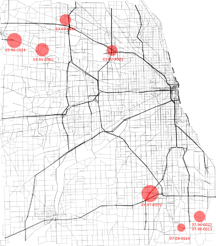
Figure 1: Potential upgrades to the Chicago Regional road network.

Project Id	Type	Cost ($000s)	Description
03-02-9005	capacity upgrade	999	add lanes on I-90 to I-294
03-03-0101	capacity upgrade	465	add lanes on Meacham Rd.
03-95-0001	new road	4000	Elgin-O’Hare Expwy to Lake St.
03-96-0024	capacity upgrade	1000	widen lanes on Villa St./Lake St.
07-06-0014	new road	472	from Cottage Grove Ave. to Mark Collins Dr.
07-94-0027	new road	700	Joe Orr Rd. extension to Burnham Ave.
07-96-0013	new road	748	Joe Orr Rd. extension to Sheffield Ave.
07-97-0055	capacity upgrade	4000	add lanes on I-57 from I-80 to I-294

Table 1: Potential upgrades to the Chicago Regional road network.

The second road network is the Berlin Center road network, used in Jahn et al. (2005). This network consists of 28 376 links, 12 981 nodes and 865 zones. We created nine hypothetical road network upgrades in this network by increasing capacity or adding roads in areas that show traffic congestion when the TAP is solved on the network with all the O-D demands from the original data doubled. These upgrades are listed in Table 2 and shown in Figure 2. Figures 3 and 4 are enlargements of the two clusters of nearby upgrades, in which each pair of upgrades is considered to be have significant pairwise interaction according to the methods described in Section 2.3.

Project Id	Type	Cost ($000s)
ber01	capacity upgrade	300
ber02	capacity upgrade	1000
ber03	capacity upgrade	800
ber04	capacity upgrade	2500
ber05	capacity upgrade	2000
ber06	capacity upgrade	4000
ber06a	new road	8000
ber10	capacity upgrade	1200
ber10a	new road	8700

Table 2: Hypothetical upgrades to the Berlin Center road network.

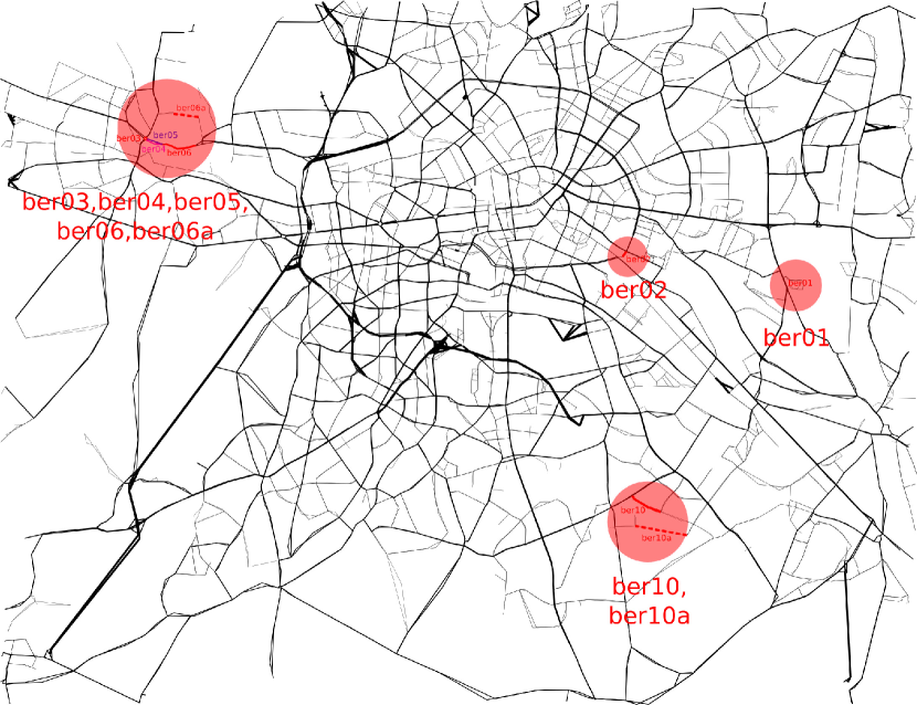
Figure 2: Hypothetical upgrades to Berlin Center road network.

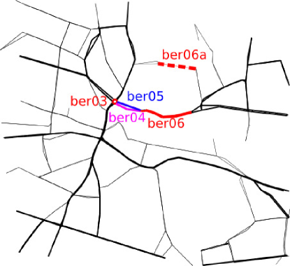
Figure 3: Detail showing a set of five significantly interacting hypothetical upgrades in the Berlin Center road network.

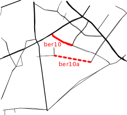
Figure 4: Detail showing a set of two significantly interacting hypothetical upgrades in the Berlin Center road network.

We used our implementation of the Frank-Wolfe method to solve the TAP on the baseline (unmodified) Chicago Regional roads network, giving the baseline total travel time of 33 657 132 VHT. This was computed after 10 000 iterations, giving a relative gap of $1.2\times 10^{-5}$. All subsequent TAP runs were computed to the same relative gap. For the Berlin Center road network, the baseline total travel time is 20 817 229 VHT, and all TAP runs are solved to a relative gap of $1.0\times 10^{-6}$.

The upgrade subset model (Equations 9–10) was written in MiniZinc and solved with the ECLⁱPS^e interval constraint solver.

In order to evaluate the accuracy of our method, we also computed the VHT resulting from solving the TAP with our implementation for the road network modified with each of the 8 individual upgrades in Table 1, as well as each of the 28 pairs of upgrades (thereby obtaining every value of $d_{ij}$ as discussed in Section 2.2), and each of the 219 subsets (with 3 or more elements) of the set of potential upgrades. The latter 219 values are used as the gold standard to evaluate the accuracy of estimating the VHT change for a set of upgrades from only individual and pairwise changes. This allows us to calculate a relative error

$$\frac{\left|\sum_{i\in S}v_{i}+\sum_{i\neq j\in S}d_{ij}-\Delta\mbox{VHT}_{S}\right|}{\Delta\mbox{VHT}_{S}}$$ (11)

where $v_{i}$ and $d_{ij}$ are as defined in Section 2.2 giving the estimate of the VHT change used in the objective function (Equation 9), and $\Delta\mbox{VHT}_{S}$ is the change in VHT computed by solving the TAP for the road network modified by all upgrades in the subset $S$ of the set of potential upgrades. This can be extended to compute the relative error when accounting for $k$-wise changes for all subsets up to (and including) size $k\leq|S|$.

Data used	$\Delta\mbox{VHT}$ computations	Mean Error %	Num Error $>10\%$
individual only	8	4.0	32
significant pairwise	9	2.4	3
all pairwise	36	0.68	2
all subsets size $\leq$ 3	92	0.25	1
all subsets size $\leq$ 4	162	0.12	0
all subsets size $\leq$ 5	218	0.043	0
all subsets size $\leq$ 6	246	0.0089	0
all subsets size $\leq$ 7	254	0.0015	0
all subsets size $\leq$ 8	255	0.0	0

Table 3: Relative error in Chicago Regional $\Delta\mbox{VHT}$ values with different degrees of upgrade interactions (sizes of subsets of upgrades) computed.

Table 3 shows the relative errors in the Chicago Regional road network for the set of upgrades in Table 1. Using all pairwise $\Delta\mbox{VHT}$ computations, we find that the mean value of this relative error is 0.68%.

If we use only the individual VHT computations, i.e. assuming all the $d_{ij}$ are 0, thereby requiring only 8 TAP computations, rather than 36 for all pairwise interactions as before, then the mean value of this relative error is 4.0%, and 32 subsets have a relative error larger than 10% (compared to only 2 when using all pairwise interactions).

If, however, we add to the individual VHT computations only the single pairwise interaction between 07-94-0027 and 07-96-0013, thereby requiring only 9 TAP computations, the mean relative error is 2.4%, and only 3 subsets have a relative error greater than 10%.

In summary, this small example shows that requiring only a single extra TAP computation, that for a pair of upgrades that a priori would be expected to have a significant difference between the sum of their individual VHT improvements and the VHT improvement resulting from implementing both, reduces the relative error from 4% to 2.4%. If we assume that the VHT improvement due to all pairwise interactions are significantly different from the sum of their individual VHT improvements, the error is reduced further, to 0.68%, however this requires a total of 36 TAP computations (an increase of 28 computations), rather than just a single extra computation.

Data used	$\Delta\mbox{VHT}$ computations	Mean Error %	Num Error $>10\%$
individual only	9	8.4	197
significant pairwise	20	1.8	16
all pairwise	45	1.8	16
all subsets size $\leq$ 3	129	0.24	0
all subsets size $\leq$ 4	255	0.038	0
all subsets size $\leq$ 5	381	0.019	0
all subsets size $\leq$ 6	465	0.0062	0
all subsets size $\leq$ 7	501	0.0013	0
all subsets size $\leq$ 8	510	0.00012	0
all subsets size $\leq$ 9	511	0.0	0

Table 4: Relative error in Berlin Center $\Delta\mbox{VHT}$ values with different degrees of upgrade interactions (sizes of subsets of upgrades) computed.

We also used the 9 individual upgrades to the Berlin Center network in Table 2, along with all 36 pairs of upgrades and 466 subsets of size 3 or greater to assess accuracy in the Berlin Center network. This example is more complex than the Chicago Regional example, in that the set of five upgrades shown in Figure 3 have a higher degree of interaction than just pairwise.

The results for the Berlin Center road network are shown in Table 4. Here we can see that the mean error of 8.4% when only individual upgrade TAP computations are used is reduced to 1.8% when all pairwise computations are used, requiring 45 TAP computations. However if only an additional 11 TAP computations (for a total of 20) are made for the two sets of significantly interacting upgrades (shown in Figure 3 and Figure 4) then the mean error is reduced to 1.8%, the same as using all pairwise computations. This example is more complex than the Chicago Regional example, in that the set of five upgrades shown in Figure 3 have a higher degree of interaction than just pairwise. As a consequence, if we use only all subsets of the interacting upgrades (those in Figures 3 and 4), then the mean error is reduced to 0.02% with 129 $\Delta\mbox{VHT}$ computations.

Table 3 and Table 4 also show that we can obtain more accuracy by solving the TAP for all subsets of increasing size, up to subset size equal to the number of individual upgrades, at which point the TAP is solved for all subsets and the error is necessarily zero. However going beyond pairwise interaction quickly leads to an impractical number of TAPs to solve, for diminishing returns. In addition, if we used higher degrees of interaction than pairwise then the objective function (Equation 9) would accordingly have a degree higher than quadratic.

Data used	$\Delta\mbox{VHT}$ computations	Mean Error %	Num Error $>10\%$
individual only	100	0.66	1
significant pairwise	145	0.22	0
all pairwise	5050	0.0	0

Table 5: Error relative to using all pairwise upgrades in Berlin Center $\Delta\mbox{VHT}$ values when using only individual upgrades versus only significant upgrade pairs.

In order to show the effectiveness of this approach on a larger scale, we generated 100 random upgrades (20 new road links and 80 roads with increased capacity) in the Berlin Center road network. Of these 100 upgrades (and therefore 4 950 pairs of upgrades), 45 pairs are considered to have potentially significant interaction by using the same distance threshold used for the Berlin Center upgrades from Table 2. We measured the error in $\Delta\mbox{VHT}$ value for each of the pairs of upgrades when solving the TAP for individual upgrades only versus solving the TAP additionally for only the upgrade pairs considered significant. The results are shown in Table 5, where it can be seen that including the 45 potentially significant pairwise computations reduces the mean error by a factor of three, and results in no pairs with a relative error greater than 10%. Note that the relative error used here is different from those used previously: due to the infeasibly large number of subsets involved, the error is measured relative not to every possible subset, but only to every pair (subset of size 2).

If we solve the model described in Section 2.2 with the Chicago Regional road network upgrades from Table 1 and a budget of $10 000 000, we find that the optimal subset of upgrades is 03-95-0001, 07-06-0014, 07-94-0027, 07-96-0013, and 07-97-0055, with net value of 168 358 (thousand dollars). There is a VHT reduction of 48 844 according to the model (using only the 8 individual and additional one significant pairwise $\Delta\mbox{VHT}$ computations), and the actual VHT reduction for this subset of upgrades is 49 794, so the model’s value has a relative error of 1.9%. Solving the model including all 3-wise interactions, thereby requiring 92 VHT computations and a cubic objective function, gives a VHT reduction of 49 927, a relative error of 0.27%.

If we solve the model with the hypothetical upgrades to the Berlin Center road network from Table 2 and a budget of $10 000 000, we find the optimal subset of upgrades is ber01, ber06a, and ber10, with net value 456 532 (thousand dollars). There is a VHT reduction of 127 679 according to the model (which is using only the 9 individual and additional 11 significant pairwise $\Delta\mbox{VHT}$ computations). The actual VHT reduction computed for this subset of upgrades is 127 653, so the model’s value has an error of only 0.02%. Solving the model using all 3-wise interactions, which requires 129 VHT computations, is enough to obtain a zero relative error in the VHT reduction for this optimal subset.

4 Finding an optimal schedule of upgrades

So far we have only considered the problem of finding the optimal subset of a set of potential upgrades, to fit in a given budget. However, a more realistic (and more difficult) problem is to find an optimal schedule of upgrades over a period of time, in which the upgrades implemented in each time period must fit within a budget for that time period. We will define “optimal” in this context shortly, but an example of a feasible schedule should help clarify the basic idea. Given the set of potential upgrades from Table 1, an example of a feasible (but not necessarily optimal) schedule is shown in Table 6. In each time period (which may be, for instance, a year, or a 5 year period), a set of upgrades that fit within that period’s budget is scheduled to be built.

Time period $t$		1	2	3	4	5	Total
Budget ($000s)		1000	4000	1500	3000	5000	14500
$i$	Project Id
1	03-02-9005	X
2	03-03-0101				X
3	03-95-0001		X
4	03-96-0024				X
5	07-06-0014				X
6	07-94-0027			X
7	07-96-0013			X
8	07-97-0055					X
Expenditure ($000s)		999	4000	1448	1937	4000	12384

Table 6: Example of a feasible road network upgrade schedule.

We will define optimality in this context as the schedule that gives the maximum net present value of VHT reductions. Recall that the present value of a monetary amount with value $c$ at time $t$ in the future is $\frac{c}{(1+r)^{t}}$ where $r$ is the interest rate. We will assume here, conventionally, that our time periods are years and the interest rate $r$ is annual, so $t$ is in years.

Using the same notation as previously (Section 2.2), but with the addition of another subscript $t$ on variables to denote their value at time $t\in\{1,2,\ldots T\}$ where $T$ is the number of time periods, the optimal schedule can be determined by the following constrained optimization problem:

$$\max\left(\sum_{1\leq t\leq T}\sum_{1\leq i<j\leq N}\frac{y_{it}y_{jt}d_{ijt}m}{(1+r)^{t}}+\sum_{1\leq i\leq N}y_{it}\left(\frac{v_{it}m}{(1+r)^{t}}-c_{i}\right)\right)$$ (12)

subject to

$$\sum_{1\leq i\leq N}y_{it}c_{i}\leq B_{t}, 1\leq t\leq T$$ (13)

$$\sum_{1\leq t\leq T}y_{it}\leq 1, 1\leq i\leq N$$ (14)

The first constraint (Equation 13) ensures that the total expenditure in each year is within that year’s budget. For convenience we can assume that all budgets and costs are expressed as their present value. The second constraint (Equation 14) states that each potential upgrade is built at most once. The example of a feasible schedule in Table 6 illustrates these constraints: the expenditure (sum of project costs) in each column is less than or equal to the budget for that time period, and each row has only one cross indicating that the project is built in only one time period.

Solving this problem exactly therefore requires not just all the individual VHT changes $v_{i}$ and pairwise changes $d_{ij}$ as in Section 2.2, but these values at all time periods $1\leq t\leq T$. They may have different values depending on which upgrades have been already built at earlier time periods, due to the effects of upgrades. In addition, although we have assumed that the O-D demand matrix is constant in a given time period, presumably it will change over time, for example increased demand generally and in between particular origins and destinations (new suburbs, for example). Hence finding the exact solution of this problem is impractical due to the factorial number of TAPs that would need to be solved (potentially we would need to solve the TAP for every permutation of feasible upgrade subsets).

We therefore propose the following heuristic “greedy” strategy to find a feasible schedule that attempts to approximate the optimal schedule. First, we choose the subset of upgrades that is optimal at the end of the entire planning period, within the total budget over all time periods. That is,

$$\max\left(\sum_{1\leq i<j\leq N}\frac{y_{i}y_{j}d_{ijT}m}{(1+r)^{T}}+\sum_{1\leq i\leq N}y_{i}\left(\frac{v_{iT}m}{(1+r)^{T}}-c_{i}\right)\right)$$ (15)

subject to

$$\sum_{1\leq i\leq N}y_{i}c_{i}\leq\sum_{1\leq t\leq T}B_{t}$$ (16)

giving a set of upgrades $U$ that will all be built by the end of the planning period. Then we need to schedule the building of these upgrades in the planning period to maximize their net present value (in terms of VHT reduction). To do so, at each time period $t\in 1,2,\ldots..T$ solve the optimal upgrade subset problem (Section 2.2, Equations 9–10), modified however to use the net present value as is done in Equation 12. That is, instead of the objective function Equation 9, use:

$$\max\left(\sum_{i,j\in U_{t},i<j}\frac{y_{it}y_{jt}d_{ijt}m}{(1+r)^{t}}+\sum_{i\in U_{t}}y_{it}\left(\frac{v_{it}m}{(1+r)^{t}}-c_{i}\right)\right)$$ (17)

where $U_{t}$ is the current set of potential upgrades (at $t=1$, $U_{t}$ is the optimal subset of upgrades $U$ for the end of the planning period obtained from solving the constrained optimization problem given by Equations 15 and 16), and the budget $B$ in Equation 10 is $B_{t}$ i.e. the budget for time period $t$ is used.

Then fix the values of $y_{ijt}$ for the current $t$, giving the subset of upgrades for time period $t$ and a new (upgraded) road network, and a new set of potential upgrades $U_{t+1}=U_{t}\setminus V$ where $V\subseteq U_{t}$ is the set of upgrades just chosen (i.e. those $i$ for which $y_{ijt}=1$). So at each time period $1<t\leq T$, the optimal upgrade subset problem is solved for the set of upgrades not yet built, using the road network determined by the upgrades chosen in period $t-1$ (and transitively by all previous time periods), and the O-D demand matrix for time $t$.

In terms of the example shown in Table 6, this heuristic algorithm can be intuitively thought of as simply choosing the optimal subset (of the set of upgrades found as optimal at the final time period given the total budget) in each time period (column) starting from the first (leftmost column), assuming in each column that the road network now has all upgrades made in previous time periods, and hence they cannot be chosen again, and that these choices are irrevocable.

When using this heuristic algorithm, we use the same values of $d_{ij}$ as in Section 4, for each time period. That is, we assume $d_{ij}=0$ unless, for the reasons discussed in Section 2.3, there is thought to be a significant difference between the sum of the VHT changes for the individual upgrades $i$ and $j$ and their pairwise VHT change, in which case $d_{ij}$ is computed by solving the TAP under the conditions prevailing at the current time period (i.e. the network including upgrades at previous time periods, and with the current O-D demand matrix).

As an alternative to the greedy heuristic, we could make stronger assumptions about the independence of the individual upgrades to reduce the complexity of the optimal upgrade schedule problem. For example, if all the upgrades are assumed to not have significant interaction (i.e. all the $d_{ij}$ are assumed to be 0), then the quadratic term in Equation 12 disappears and the TAP only needs to be solved for each individual upgrade at each time period. However, we would expect, given the results discussed in Section 3, that ignoring these interactions entirely could lead to significant errors in VHT reduction estimates and therefore potentially very far from optimal schedules.

These algorithms demonstrate a shortcoming of the Frank-Wolfe method that we have been using. Some algorithms such as Origin-Based Assignment (OBA) (Bar-Gera, 2002) and Algorithm B (Dial, 2006) can “warm start” from a converged TAP solution with a changed O-D demand matrix and reach equilibrium more quickly than if started from scratch. Frank-Wolfe does not have this ability and hence OBA or Algorithm B may be useful in the situation where we solve the TAP for a number of modified networks with a given O-D demand matrix, and then need to re-solve it with a changed O-D demand matrix in order to find the baseline VHT for the next scheduling period. They will not necessarily be an improvement in the majority of cases where we need to solve the TAP again with a modified network, but obviously any improvement in the speed with which the TAP can be solved is useful.

4.1 Results

We implemented the heuristic algorithm by writing the models (Equations 15–17) in MiniZinc and solving with the ECLⁱPS^e interval constraint solver, and using a scripting language to run the solvers with the appropriate data at each iteration.

We used the eight upgrades to the Chicago Regional road network listed in Table 1, with the five time periods and budgets for each as in the example schedule in Table 6. We used the Chicago Regional data, identical to that previously used in the first time period. For the subsequent time periods, we re-ran the TAP for all modifications with a 10% increase in trips to and from the CBD and a 15% increase in trips to and from O’Hare airport in each period. We used the factor $m=3650$ to convert VHT to dollars and an annual interest rate of 4%. The resulting schedule is shown in Table 7. If all the upgrades were built at the end of the planning period (i.e. the first step of the greedy heuristic, where we find a subset that is optimal at the end, within the total budget over all periods), then the dollar present value of the VHT reduction (in thousands of dollars) is 148 151, while the net present value of the schedule shown in Table 7 is 164 359.

Time period $t$		1	2	3	4	5	Total
Budget ($000s)		1000	4000	1500	3000	5000	14500
$i$	Project Id
1	03-02-9005
2	03-03-0101				X
3	03-95-0001		X
4	03-96-0024
5	07-06-0014			X
6	07-94-0027			X
7	07-96-0013	X
8	07-97-0055					X
Expenditure ($000s)		748	4000	1172	465	4000	10385

Table 7: Road network upgrade schedule for the Chicago Regional road network generated by the greedy heuristic algorithm.

For comparison, we used the same data in the simplified model that assumes independence of all upgrades. As previously mentioned, this means that the quadratic term in Equation 12 disappears, giving the following linear constrained optimization problem:

$$\max\left(\sum_{1\leq t\leq T}\sum_{1\leq i\leq N}y_{it}\left(\frac{v_{it}m}{(1+r)^{t}}-c_{i}\right)\right)$$ (18)

subject to

$$\sum_{1\leq i\leq N}y_{it}c_{i}\leq B_{t}, 1\leq t\leq T$$ (19)

$$\sum_{1\leq t\leq T}y_{it}\leq 1, 1\leq i\leq N$$ (20)

It is practical to solve this exactly (again by writing the model in MinZinc and solving with the ECLⁱPS^e interval constraint solver) as the assumption of the independence of all the upgrades means we need only solve the TAP for each individual upgrade at each time period (each subsequent time period having increased O-D demands as described above). The resulting upgrade schedule is shown in Table 8.

This schedule has a net present value (in thousands of dollars) of 145 648 according to the model, and actual NPV (computed by solving the TAP for each upgrade at each period according to the schedule and then computing the NPV of the upgrades) of 164 091.

Time period $t$		1	2	3	4	5	Total
Budget ($000s)		1000	4000	1500	3000	5000	14500
$i$	Project Id
1	03-02-9005
2	03-03-0101			X
3	03-95-0001		X
4	03-96-0024
5	07-06-0014				X
6	07-94-0027					X
7	07-96-0013	X
8	07-97-0055					X
Expenditure ($000s)		748	4000	465	472	4700	10385

Table 8: Road network upgrade schedule for the Chicago Regional road network generated by solving the linear model assuming independence of all upgrades.

Both of these schedules are improvements on the example schedule in Table 6, however, which has a a net present value of 157 676 (thousand dollars).

This example demonstrates that the greedy heuristic algorithm, using information about pairwise interaction between upgrades, is capable of finding better upgrade schedules than the exact solution of the simplified upgrade scheduling problem in which pairwise interactions are ignored.

5 Conclusions

In this paper, we have demonstrated a method to find the optimal subset of a set of potential road network upgrades, without having to solve the traffic assignment problem for each subset. Although this may be necessary in principle, we have shown that reasonable approximations can be achieved by considering only those pairs of upgrades that potentially have significant interactions. This subset of pairs can be predicted with a simple distance threshold or clustering technique. In addition, we have shown how to find an implementation schedule of the upgrades to maximize the net present value of the reduction in vehicle hours travelled over the planning period.

It should be noted that many major simplifications have been made in this modelling process. Perhaps most importantly, we have assumed that the single optimization objective is to minimize vehicle hours travelled, a value determined entirely by the flow on the road network at user equilibrium, given a fixed origin-destination demand matrix. However there may be important other benefits, or drawbacks, to a particular road upgrade, such as social and environmental costs (or benefits), or financial or political considerations relating to building roads or operating toll roads for example, that are not accounted for. If, as is done in Section 4, the VHT value is converted to a monetary value (by assigning a monetary cost to each vehicle hour — and here different types of traffic such as personal, work-related, commercial freight, etc. should be distinguished), and if externalities are also converted to monetary costs, then they could be incorporated as costs or benefits in a more sophisticated model, however that is beyond the scope of this work.

We have also simplified somewhat by considering only road traffic assignment, ignoring mode choices where such alternatives as public transport exist. Traffic assignment is usually used as one step in an iterative multi-step process including mode choice and trip generation: this multi-step process could be used in place of the simple traffic assignment described here to incorporate different transport modes into the model.

By using a conventional static traffic assignment model, where flow on a link is allowed to exceed its capacity when congested, we have ignored the possibility of demand being affected by congestion. Some more sophisticated models can address this, such as “stationary dynamic” models (Nesterov and de Palma, 2003) in which excess demand is queued, or elastic demand models (Babonneau and Vial, 2008), in which demand for travel between an origin and destination is a function of travel costs. Further, by using a static model with fixed origin-destination demand, we have ignored any induced demand that may result from improving travel times, or at least deferred this to the separate problem of estimation of demand in the future.

6 Acknowledgements

We have been greatly assisted in this work by the public availability of the transportation network test problems, TAP file format, and sample TAP code from Dr Hillel Bar-Gera. This research made use of the Victorian Partnership for Advanced Computing HPC facility and support services. NICTA is funded by the Australian Government as represented by the Department of Broadband, Communications and the Digital Economy and the Australian Research Council through the ICT Centre of Excellence Program.

References

- Babonneau and Vial (2008) Babonneau, F., Vial, J.P., 2008. An efficient method to compute traffic assignment problems with elastic demands. Transportation Science 42, 249–260.
- Bar-Gera (2002) Bar-Gera, H., 2002. Origin-based algorithm for the traffic assignment problem. Transportation Science 36, 398–417.
- Bar-Gera (2010) Bar-Gera, H., 2010. Transportation network test problems. http://www.bgu.ac.il/~bargera/tntp/. Accessed 16 December 2010.
- Beckmann et al. (1956) Beckmann, M.J., McGuire, C.B., Winsten, C.B., 1956. Studies in the Economics of Transportation. Yale University Press, New Haven.
- Bellman (1957) Bellman, R., 1957. Dynamic Programming. Princeton University Press, Princeton, New Jersey.
- Bertsekas (1993) Bertsekas, D.P., 1993. A simple and fast label correcting algorithm for shortest paths. Networks 23, 703–709.
- Bertsekas et al. (1996) Bertsekas, D.P., Guerriero, F., Musmanno, R., 1996. Parallel asynchronous label-correcting methods for shortest paths. Journal of Optimization Theory and Applications 88, 297–320.
- Brisset et al. (2011) Brisset, P., El Sakkout, H., Früwirth, T., Gervet, C., Harvey, W., Meier, M., Novello, S., Le Provost, T., Schimpf, J., Shen, K., Wallace, M., 2011. ECLiPSe Constraint Library Manual. release 6.0 edition. http://www.eclipseclp.org/doc/userman.pdf accessed 17 October 2011.
- (9) Caliper, 2011. Caliper transcad. http://www.caliper.com/tcovu.htm. Accessed 17 October 2011.
- (10) Chicago Metropolitan Agency for Planning, 2011. Chicago metropolitan agency for planning transportation improvement program (tip). http://www.cmap.illinois.gov/tip. Accessed 12 May 2011.
- (11) Citilabs, 2011. Citilabs. http://citilabs.com. Accessed 17 October 2011.
- Dafermos and Sparrow (1969) Dafermos, S.C., Sparrow, F.T., 1969. The traffic assignment problem for a general network. Journal of Research of the National Bureau of Standards — B. Mathematical Sciences 73B, 91–118.
- Dial (2006) Dial, R.B., 2006. A path-based user-equilibrium traffic assignment algorithm that obviates path storage and enumeration. Transportation Research Part B 40, 917–936.
- Dijkstra (1959) Dijkstra, E.W., 1959. A note on two problems in connexion with graphs. Numerische Mathematik 1, 269–271.
- Florian and Hearn (1995) Florian, M., Hearn, D., 1995. Chapter 6 network equilibrium models and algorithms, in: Ball, M., Magnanti, T., Monma, C., Nemhauser, G. (Eds.), Network Routing. Elsevier. volume 8 of Handbooks in Operations Research and Management Science, pp. 485 – 550.
- Ford and Fulkerson (1965) Ford, L.R., Fulkerson, D.R., 1965. Flows in networks. Princeton University Press, Princeton, New Jersey.
- Frank and Wolfe (1956) Frank, M., Wolfe, P., 1956. An algorithm for quadratic programming. Naval Research Logistics Quaterly 3, 95–110.
- Fredman and Tarjan (1987) Fredman, M.L., Tarjan, R., 1987. Fibonacci heaps and their uses in improved network optimization algorithms. Journal of the Association for Computing Machinery 34, 596–615.
- Gentile (2009) Gentile, G., 2009. Linear User Cost Equilibrium: a new algorithm for traffic assignment. Technical Report. Sapienza Università di Roma.
- Jahn et al. (2005) Jahn, O., Möhring, R.H., Schulz, A.S., Stier-Moses, N.E., 2005. System-optimal routing of traffic flows with user constraints in networks with congestion. Operations Research 53, 600–616.
- Jayakrishnan et al. (1994) Jayakrishnan, R., Tsai, W.K., Prashker, J.N., Rajadhyaksha, S., 1994. Faster path-based algorithm for traffic assignment. Transportation Research Record 1443, 75–83.
- Klunder and Post (2006) Klunder, G.A., Post, H.N., 2006. The shortest path problem on large-scale real-road networks. Networks 48, 182–194.
- LeBlanc et al. (1975) LeBlanc, L.J., Morlok, E.K., Pierskalla, W.P., 1975. An efficient approach to solving the road network equilibrium traffic assignment problem. Transportation Research 9, 309–318.
- Nesterov and de Palma (2003) Nesterov, Y., de Palma, A., 2003. Stationary dynamic solutions in congested transportation networks: Summary and perspectives. Networks and Spatial Economics 3, 371–395.
- Nethercote et al. (2007) Nethercote, N., Stuckey, P.J., Becket, R., Brand, S., Duck, G.J., Tack, G., 2007. MiniZinc: Towards a standard CP modelling language, in: Bessiere, C. (Ed.), Principles and Practice of Constraint Programming — CP 2007, pp. 529–543.
- Pape (1974) Pape, U., 1974. Implementation and efficiency of Moore-algorithms for the shortest route problem. Mathematical Programming 7, 212–222.
- Patriksson (1994) Patriksson, M., 1994. The Traffic Assignment Problem: Models and Methods. VSP BV, Utrecht.
- (28) PTV AG, 2011. Ptv ag. http://ptvag.com. Acessed 17 October 2011.
- Rose et al. (1988) Rose, G., Daskin, M.S., Koppelman, F.S., 1988. An examination of convergence error in equilibrium traffic assignment models. Transportation Research Part B 22B, 261–274.
- Schimpf and Shen (2010) Schimpf, J., Shen, K., 2010. Eclipse - from lp to clp. CoRR abs/1012.4240. http://arxiv.org/abs/1012.4240.
- Sheffi (1985) Sheffi, Y., 1985. Urban Transportation Networks: Equilibrium Analysis with Mathematical Programming Methods. Prentice-Hall, Englewood Cliffs, N.J.
- Slavin et al. (2006) Slavin, H., Brandon, J., Rabinowicz, A., 2006. An empirical comparison of alternative user equilibrium traffic assignment methods, in: Proceedings of the European Transport Conference 2006.
- Wu et al. (2011) Wu, D., Yin, Y., Lawphongpanich, S., 2011. Optimal selection of build-operate-transfer projects on transportation networks. Transportation Research Part B Article in Press, Corrected Proof, http://dx.doi.org/10.1016/j.trb.2011.07.006.
- Zhan and Noon (1998) Zhan, F.B., Noon, C.E., 1998. Shortest path algorithms: An evaluation using real road networks. Transportation Science 32, 65–73.