(Hardware: 4 worker nodes w/ $2\times$RTX8000, low-end head node, 10-Gigabit Ethernet, screen size $2560\times 1080$)
PBRT landscape: max 3.7 GB GPU usage, 6.2 FPS (1 path/pixel)	Disney Moana island: max 25 GB GPU usage, 7.9 FPS (1 path/pixel)
30 K instances, 4.3 B inst. triangles, 370 unique meshes, 500 MB image textures	39 M instances, 41 B inst. triangles, 7 M unique meshes, 804 MB baked-PTex txt.

Figure 1. Two screenshots from a data-parallel path tracer built using the techniques described in this paper; showing multi-bounce path tracing, textures, alpha textures, area- and environment lighting, etc., on two non-trivial models each distributed across 4 nodes and 8 GPUs. Despite intentionally low-end network infrastructure, at $2560\times 1080$ pixels and one path per pixel these two examples run at 6.2 and 7.9 frames per second, respectively (images shown are converged over multiple frames).

Data Parallel Path Tracing in Object Space

Abstract.

We investigate the concept of rendering production-style content with full path tracing in a data-distributed fashion—that is, with multiple collaborating nodes and/or GPUs that each store only part of the model. In particular, we propose a new approach to tracing rays across different nodes/GPUs that improves over traditional spatial partitioning, can support both object-space and spatial partitioning (or any combination thereof), and that enables multiple techniques for reducing the number of rays sent across the network. We show that this approach can handle different kinds of model partitioning strategies, and can ultimately render non-trivial models with full path tracing even on quite moderate hardware resources with rather low-end interconnect.

1. Introduction

Data-parallel (or data-distributed) rendering is the process of rendering a model whose constituent components are distributed across the memories of multiple different compute units such as HPC compute nodes or GPUs (which, following MPI parlance, we will often call ranks). This is typically done for one of two reasons: one is that a given model is too large to fit into the memory of a single node, and the user chooses to distribute it across several different nodes (we call this explicit distribution); the second is that for some reason or other the model’s data is already spread across different nodes, and cannot easily be merged for rendering (i.e., it is natively distributed). Data-parallel rendering did attract some attention in the past, but in practice today it is almost entirely confined to scientific visualization (sci-vis), and even there is almost only performed with image compositing-based approaches that cannot handle effects like path tracing. For the kind of images shown in Figure 1, data parallel rendering today is virtually non-existent. The list of possible explanations for that is long, and a full discussion beyond the scope of this paper. However, we argue that these reasons can be sorted into either one of two groups: one that argues that there is neither need nor demand for data-parallel rendering in production rendering; and one that argues that it is too hard.

For the first one, we argue that data is increasingly moving into the cloud (where parallel resources are easily available), and that content is continuing to grow at a rate that far surpasses the rate at which GPU or even host memories are growing. The second is more interesting, as the data parallel rendering techniques we use in sci-vis today may indeed not be ideally suited for this context: First, sci-vis rendering largely relies on image compositing, but for path tracing we certainly can not. Path tracing requires the frequent forwarding of either rays or data between nodes; and that is expensive. Second, the content used in production rendering is very different than that encountered in visualization, including spatially large yet hard to split instances or meshes with shading data, abundant spatial overlap, etc. As we show below this content does not always do well with spatial subdivision, yet this is what virtually all data-parallel rendering today is built on.

In this paper, we take a closer look at data-parallel path tracing for production style content. In particular, we borrow some of the last few years’ insights on ray tracing acceleration structures, and use that to propose several new techniques that go beyond strictly spatial scene subdivisions. We do this through a combination of two things: First, we describe distributed content through what we call proxies–bounding boxes that describe which parts of the model can be found on which rank(s), and which are allowed to arbitrarily overlap any other proxies. Second, we propose an object-space parallel ray forwarding operator that—using those proxies—enables each ray to easily determine which node/GPU it should next be forwarded to. We describe several techniques that make this efficient, and demonstrate this using a prototype data parallel path tracer built using these techniques (Figure 1).

2. Related Work

Parallel rendering refers to a family of methods where multiple nodes and/or GPUs work together to render one model; data-parallel rendering to where every node has only part of the model. Throughout this paper we adopt the parlance of the Message Passing Interface (MPI) [Gropp et al., 1999; Walker and Dongarra, 1996], referring to ranks in groups that can communicate with each other through the passing of messages. MPI can also run multiple ranks on the same node, but we will typically use one rank per GPU.

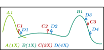
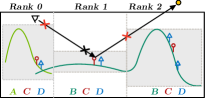
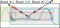
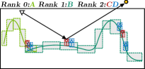
Figure 2. The core ideas behind our method, illustrated on a 2D sketch of a model very like the island model. a) Our model consists of two base meshes (A and B), and three respectively four instances of two types of tree (C and D). b) spatial partitioning on this model runs into two issues: it struggles to properly partition it with spatial splits, and it can end up with large boxes that incur ray forwarding between ranks. c) Object space partitioning allow for non-spatial scene partitions, but if done naively ends up with even worse ray traffic. d) we represent objects by more than one—possibly overlapping, but tight-fitting—”proxies”: these are more flexible and general than either spatial or object space techniques, and also require less forwarding.

Today, data parallel rendering is almost entirely confined to svi-vis, with packages like ParaView [Ahrens et al., 2005] and VisIt [Childs et al., 2012] handling the data distribution, and communication-optimized libraries such as Ice-T [Moreland, 2011] handling the compositing. This is used for both volumetric and polygonal data, but is generally restricted to simple shading where alpha- or Z-compositing can be used. Sci-vis also uses path tracing, but in this case usually relies on data replicated rendering.

In a ray tracing context, parallel rendering is easiest to realize when using either replicated rendering [Wald et al., 2020; Xie et al., 2021]. Approaches to dealing with models larger than available memory can be classified into three categories: out of core ray tracing, where data is paged in on demand, usually including some form of batching, sorting, scheduling, and caching [Pharr et al., 1997; Burley et al., 2018]; data forwarding, where data is sent to / fetched by whatever node needs it [Wald et al., 2001; DeMarle et al., 2004; Ize et al., 2011; Jaros et al., 2021]; and ray forwarding where rays get scheduled on, and sent to, other node(s) [Salmon and Goldsmith, 1989; Reinhard, 1995; Kato and Saito, 2002; Park et al., 2018; Abram et al., 2018].

An interesting exception to this classification is the concept of hardware-assisted distributed shared memory as recently used by Jaros et al.’s [2021], in their case using CUDA unified memory and NVLink on an NVidia DGX: on the hardware level this uses data-forwarding over high-bandwidth NVLink, with unified memory giving the appearance of a single replicated address space; on the software side, the authors show that best performance is achieved if the application is aware of which data lives on which physical GPU, and ideally even replicates some of that data.

Looking at the literature on data parallel ray tracing we make two observation: First, that the ray forwarding approach has received but scant attention: some early work has looked at the scheduling part of the problem (see, e.g., [Reinhard, 1995] for an overview), but we are aware of only three somewhat-recent approaches that actually forward rays: The Kilauea renderer [Kato and Saito, 2002] (which simply forwarded every ray to every node), Park’s SpRay system [2018] (which focuses primarily on scheduling and speculative execution), and TACC’s Galaxy [Abram et al., 2018] (which uses techniques similar to those in SpRay). Second, across all the different approaches to data parallel rendering taken over the last four decades researchers seem to have taken it for granted that data would necessarily get spatially partitioned using various forms of grids, octrees, kd-trees, etc. The latter is particularly striking given the last decade’s lively discussion around spatial vs object hierarchies in ray tracing. In this field, the community has largely switched from spatial techniques to object-space techniques like BVHes [Parker et al., 2010; Wald et al., 2014; Burgess, 2020]. These BVHes are often built using spatially influenced techniques like top-down partitioning and the Surface Area Heuristic (SAH) [Karras and Aila, 2013]), and do best when augmented with optimizations like spatial splits [Stich et al., 2009; Ganestam and Doggett, 2016; Ernst and Greiner, 2007] and braiding [Benthin et al., 2017]—but they are nevertheless object-space techniques.

Issues with spatial partitioning have also been pointed out by Zellmann et al. [2020]. They proposed techniques that produce better spatial partitions, but never went beyond spatial partitions.

3. Data Parallel Ray Traversal

In this section, we will give a high-level overview of the general concepts and techniques for what we call data-parallel ray traversal in object space. The core idea is to combine two things: first, a more general representation of data-distributed scene content where different pieces of content across different nodes are allowed to spatially overlap other such content, both on the same and/or other nodes; or even to be replicated across multiple nodes if and where desired. Second, the concept of what we call a data-distributed forwarding operator that, in the presence of such object-space distributed content can always tell which other node a given ray needs to be forwarded to next, in a guaranteed correct yet efficient manner that explicitly aims to minimize the number of times that such forwarding needs to happen.

3.1. Goals, Non-Goals, and Key Issues

Our goal is to render—with full path tracing—models that are larger than the memory of any one of our ranks (and in general, larger than the host memory of the nodes that contain these GPUs). We explicitly target assets similar to the island model that—at least with a good partitioner—may today need only on the order of four or eight GPUs; not the “at scale” type visualizations of up to thousands of nodes that are so common in visualization. While we do believe our method will also work in larger scenarios these are not currently our focus; nor is the concept of strong vs weak scaling that is so important in sci-vis.

We also observe that such content is very different that encountered in sci-vis. For example, spatial overlap of different logical objects and instances is not just a possibility, but a given.

While we do aim for interactive performance, we do not (yet) aim for fully real-time photo-realistic rendering. We do believe our method to be a first step towards this goal, but this will ultimately require more systems work than entertained in this paper. We expect network bandwidth to be the ultimate bottleneck, but we still need to perform a fair amount of shading and texturing. Thus, though our framework can also be recompiled to a CPU-only backend using Embree for this paper we only consider GPUs.

With the growing gap between compute and bandwidth our main concern is to reduce the amount of network bandwidth required for a given frame. This can lead to un-intuitive situations: in data replicated rendering one can expect that adding more resources will improve performance, but in data-parallel the opposite is often the case—adding more ranks also increases the chance that rays need to get forwarded, which is counter-productive.

3.2. Core Idea

With these goals in mind, let us take a look at how state of the art data-parallel ray tracing would work for the kind of content we are targeting: Let us consider a simplified example of a 2D ”island” model shown in Figure 2a: a model made of two base meshes, with two types of trees that each have several instances.

Let us now first consider the state of the art, and let us create an imaginary spatial partitioning of this model into three disjoint regions (Figure 2b): no matter where exactly the splits are placed in this example, almost every spatial domain is overlapped by almost every base mesh, and contains at least one copy of each type of tree. Though the number of instances in each region has decreased, memory per node barely has. Let us now also look at two hypothetical rays as shown in Figure 2b: traversing these rays across those spatial domains is obvious and trivial, but each of these rays touches two ranks, despite not even being close to any of the geometry in the first or last rank (this only gets worse in 3D).

Let us now consider that same model with a purely object-space partitioning, and simply assign the first mesh to one rank, the second to another, and all instances of all trees to the third (Figure 2c). Replication is now gone completely, but overlapping boxes mean that rays are now touching even more ranks’ data; and traversal order is no longer obvious. Now let us take this general idea, but apply some ideas from the last decade’s discussion on BVHes vs kd-trees; in particular, concepts such as spatial splits [Stich et al., 2009; Ganestam and Doggett, 2016] and braiding [Benthin et al., 2017] to reach “into” large instances, and instead represent them with several individual, tight-fitting bounding boxes. If we do this (Figure 2d) an indeal algorithm could now—if it existed—trace both of these rays on the same rank, without any ray forwards at all.

3.3. Proxies and Data-Distributed Traversal

Our initial plan to realize the ideas sketched in the previous section was to assign each instance to exactly one rank, to create exactly one proxy per instance, and to have each rank build exactly the same BVH over those proxies. This suggests an obvious BVH-style traveral through those proxies, sending rays to the nodes that owned the proxies they traversed. To have the next node continue traversal where the previous one left off we had planned on using a stack-free BVH traversal such as described by Hapala [2011] or Vaidyanathan [Vaidyanathan et al., 2019]. This is indeed a useful mental picture of how our method works; however, we can significantly improve upon this as described in the rest of this section.

3.3.1. Traversing nodes, not instances.

Once a ray hitting a given proxy is sent to the node owning that proxy there is no reason to limit intersection to that one instance that generated that proxy. Local geometry intersection is cheap compared to sending a ray over the network, so we should always intersect all geometry on that node. Once we do that we want to make sure that no matter which proxies a ray encounters it will never be sent to the same node twice. This requires tracking the nodes a ray has already visited; we present two options for that below.

3.3.2. Front to back traversal.

A stack-free BVH-style traversal of the proxies sounds easy, but in a distributed context it isn’t, as even minute differenced in different ranks’ BVHes could lead to infinite loops; nor would it guarantee front-to-back traversal. If, however, rays do keep track of which nodes they have already visited, then we can do something that is even simpler: we simply trace the ray into those proxies, and find the closest such proxy that belongs to a node that we have not yet traversed.

landscape		island
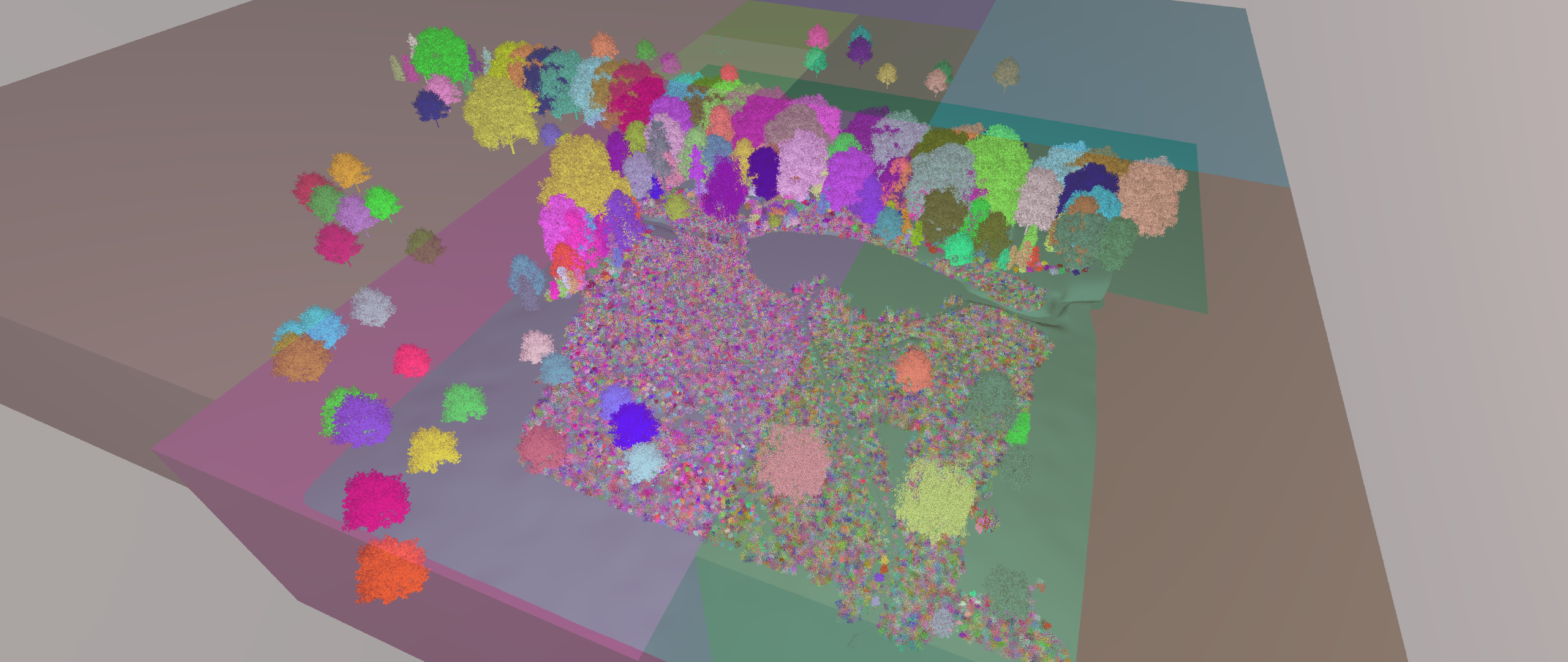
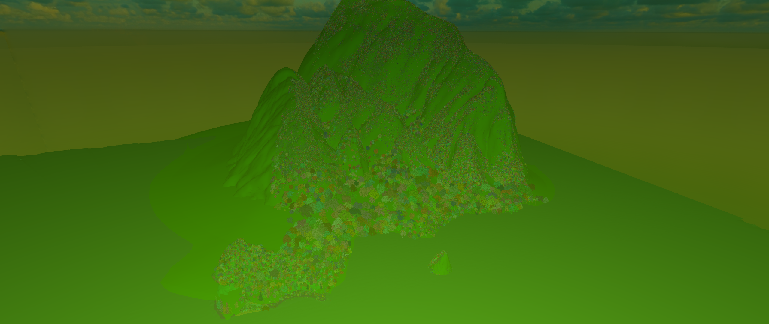
spatial (median)	spatial (w/ cost fct)	spatial (median)	spatial (w/ cost fct)
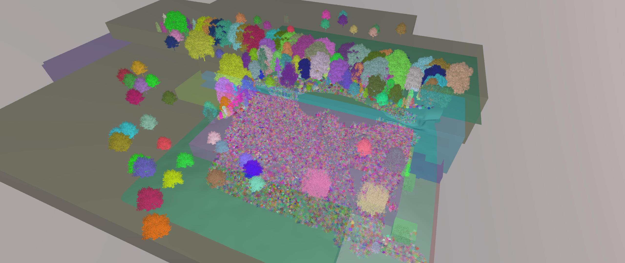
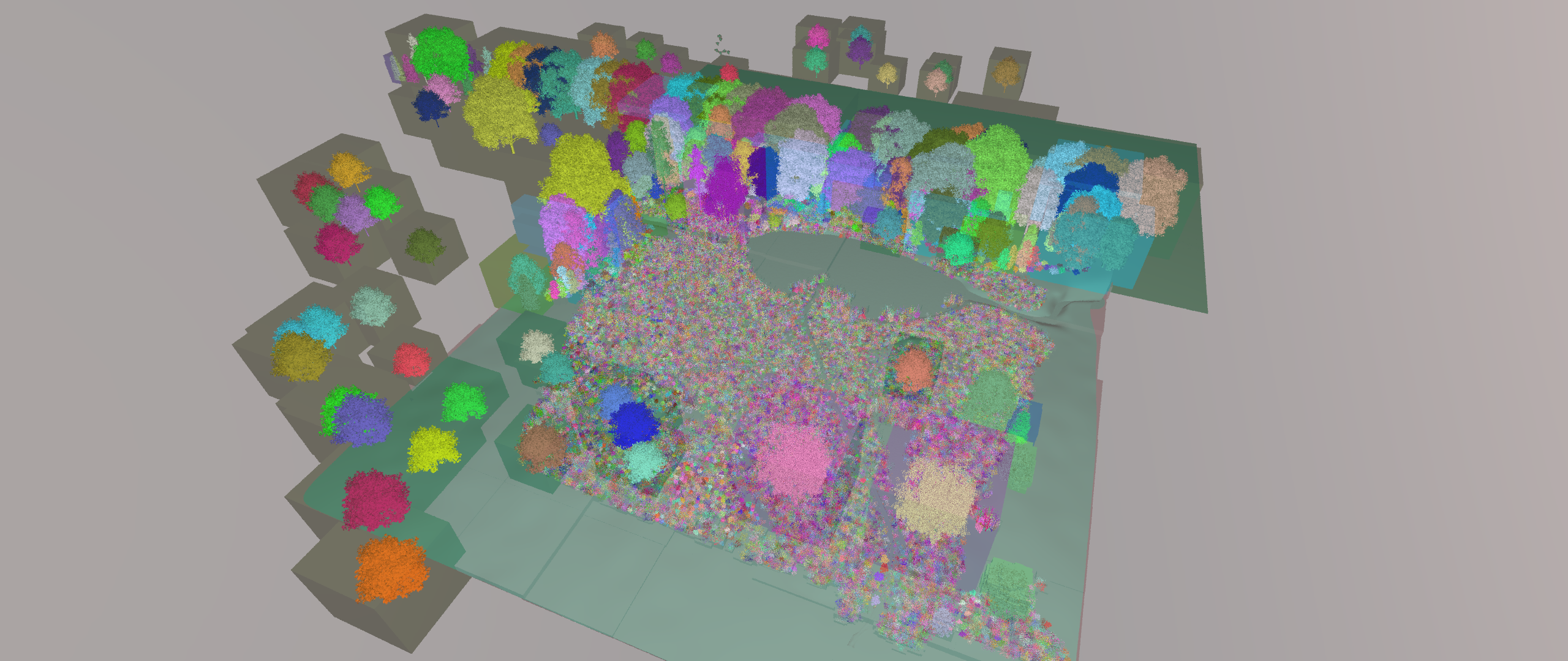
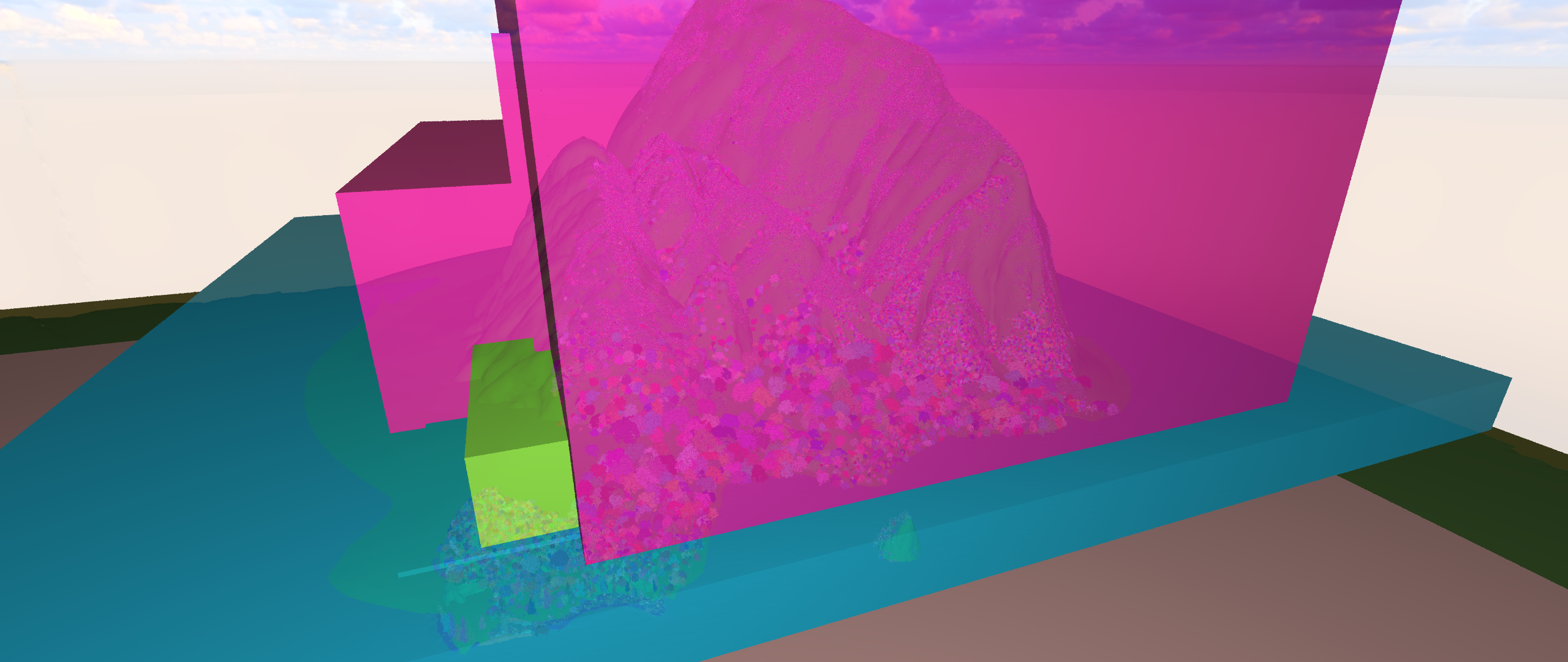
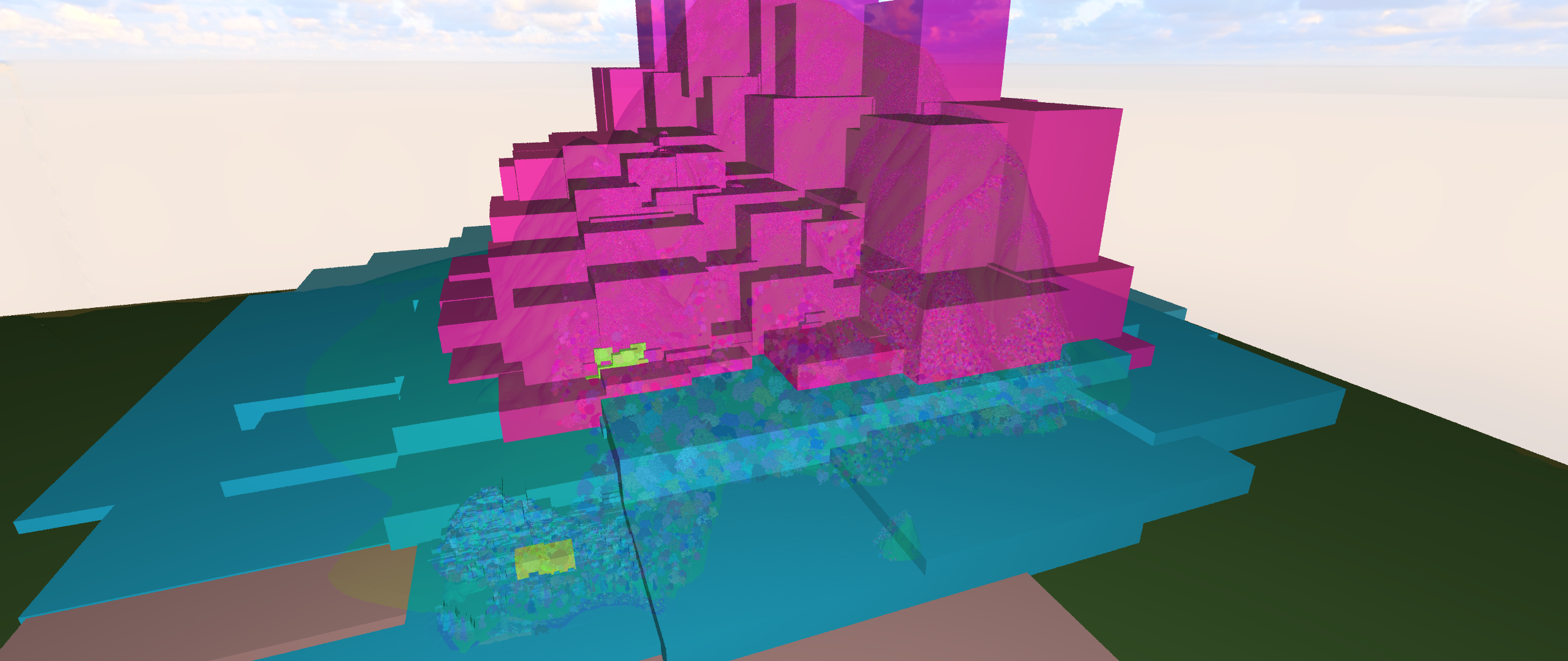
object (naive)	object (+ proxies)	object (naive)	object (+ proxies)
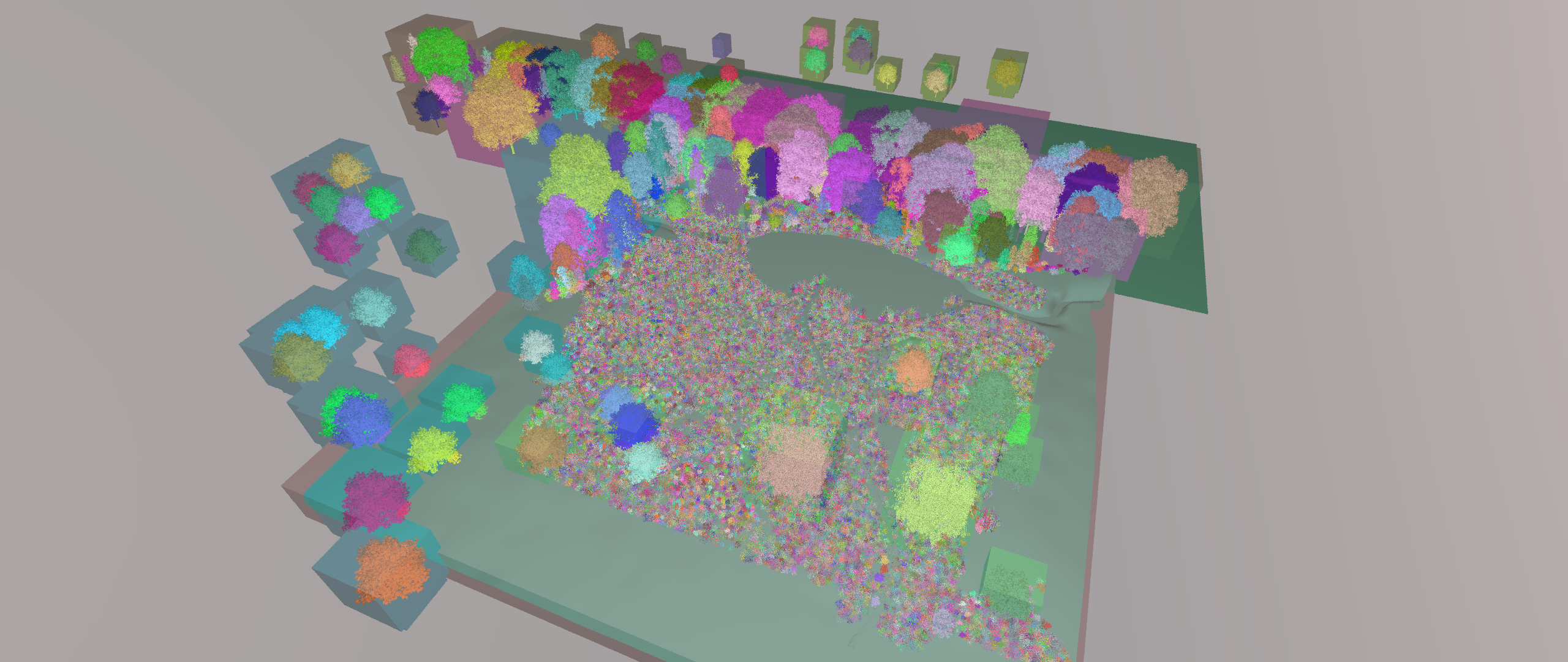
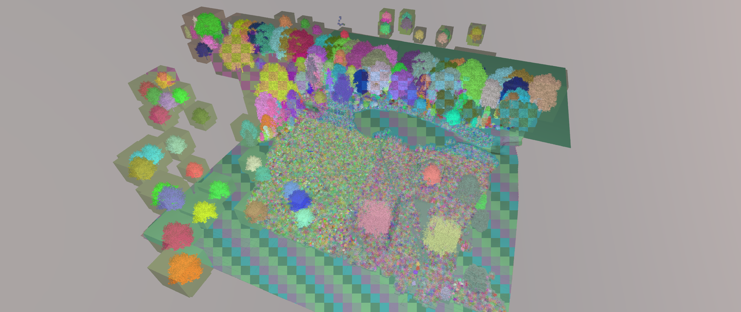
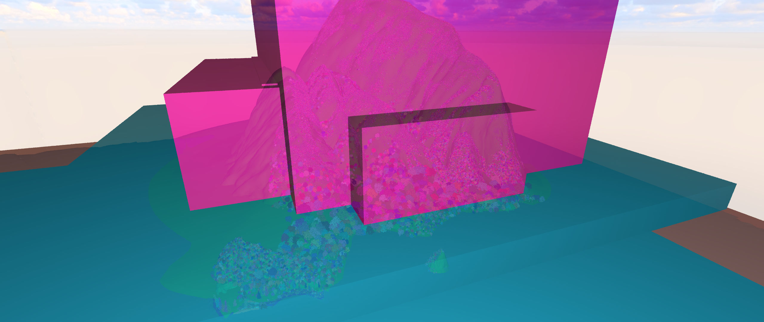
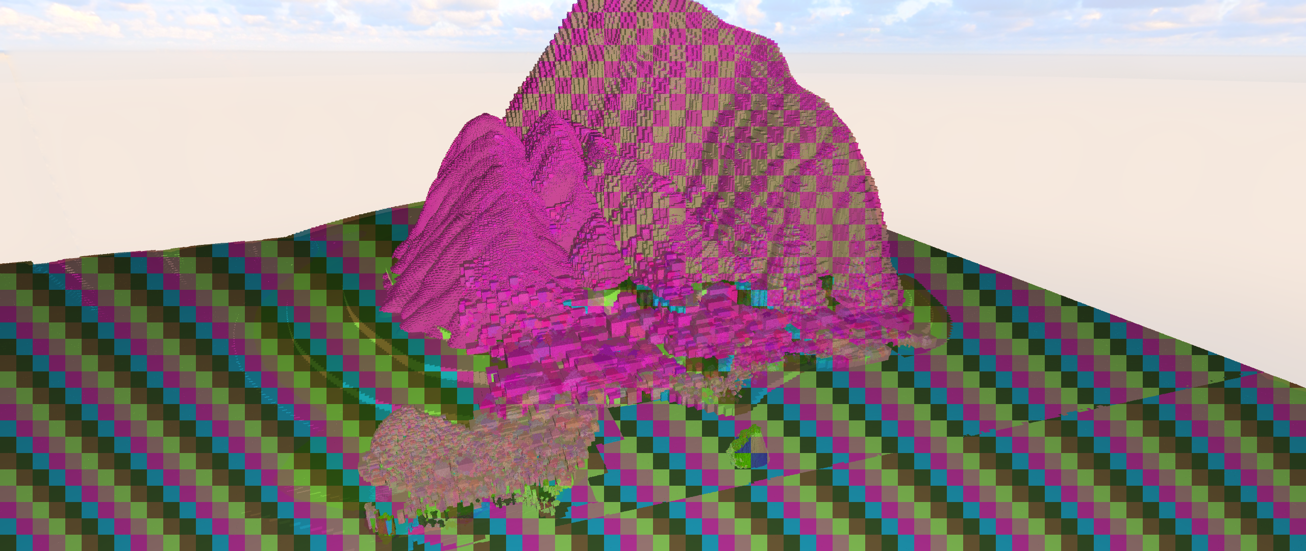
bvh-like	best (w/ some replication)	bvh-like	best (w/ some replication)

Figure 3. Visual depiction of the model partitions that our sample partitioners produce for both landscape and island, with the boxes showing the used proxies’ bounding boxes, and their color encoding the rank they are on (proxies with same color are on the same rank). Proxies with a checkerboard pattern mean that this content is owned on more than one rank.

3.3.3. Intersection local geometry.

For a newly spawned secondary ray, even front-to-back traversal does not guarantee that the spawning rank will get picked first; yet at some time that ray would certainly get sent to that node. We always first trace each ray on their generating ranks, then tag it as having already visited this rank. In particular for shadow rays there is a good chance that this new ray can actually find an occluder on that same node, and never has to leave that rank at all.

3.3.4. Generalizing proxies.

Creating exactly one proxy per instance can lead to very large proxies for some objects, which in turn would require lots of rays to be sent to that node. We observe that this is very similar to problems that have recently been investigated for BVH traversals, and in particular point to techniques like spatial splits and braiding. Both of these work by representing spatially large objects in a BVH through more than one box, with the entirety of these boxes covering the object more tightly than one single box. We use this to conservatively but tightly represent spatially large instances with multiple smaller boxes (see Figure 2d), which allows rays to pass around some geometry whose proxies they would otherwise have hit. Rays can now encounter multiple proxies of the same object, but the previous paragraphs’ techniques skip these, so this is OK. Ultimately this means that proxies no longer represent any particular instance, but just a region of space that a given node has content for. I.e., we can have one proxy represent more than one instance, or use multiple proxies for the same instance, etc.

3.3.5. Replicating certain geometry.

Just like proxies are not tied to any particular instance, so we can generalize the concept of who owns the content behind one proxy. Though we did initially assign exactly one rank to every instance, for some spatially large (and thus, likely to get traversed) yet not memory intensive object(s) we might also want to replicate this object to more than one node, such that rays already on that node would have it available without needing to travel to the node owning it. With our proxies, we can easily do that, by allowing proxies to specify that whatever it may represent, it can be found on more than one node. The traversal logic above does not change at all: when we trace a ray to find the next proxy we simply reject all proxies for which the ray has been to any of the nodes listed in that proxy.

3.3.6. Proxy-guided primary ray generation.

Above we have described that secondary rays should always be traced on the node that spawned them, but for primary rays we can actually choose where to spawn them. In particular, we can use our proxies to generate each path on exactly the node that owns the closest proxy for the given pixel, thus maximizing the chance that this ray will find its first intersection on exactly the node it was generated on.

3.3.7. Tracking which nodes a ray has already been on.

In all of the previous techniques we have made the implicit assumption that a ray always known which node(s) it has already been on. For not too large a number of ranks this can be realized through a bit mask (with one bit per rank) that gets attached to each ray. For a large number of ranks this would lead to an explosion in ray size; however, this can be avoided by what we call the “replay” technique: if each ray only ever stores which rank it was generated on, then any node can later re-compute the actual set of visited nodes by simply re-running the above logic until it reaches itself.

In combinations these technique provide a very effective operator that—using only the proxies, the ray, and the ray’s stored history—allows any node to robustly and efficiently determine which other rank to forward that given ray to next; if this comes up empty that ray’s distributed traversal is complete.

4. Partitioning

This paper is not about one particular partitioning strategy; in fact, we believe our method’s greatest strength is its ability to express and handle distributed content in a more general way. To demonstrate this flexibility we implemented multiple different partitioners, including both spatial, object space, and hybrid methods. All our variants work similarly in that we start by creating one part containing the whole scene, then iteratively take the respectively largest part, and split that into two. For objects with more than one instance we use the individual instances of that object, for those with only one instance we follow Zellmann [2020] and break that object into its constituent meshes.

Spatial partitioning starts with an initial domain set to the scene’s bounding box, and in each split creates two non-overlapping halves, then checks which objects overlap each half’s domain. Again following Zellmann, after each step each side’s domain gets shrunk to the content it contains, if possible. For deciding where to split we implemented two methods: spatial-simple splits each domain at its spatial median; spatial-sah uses a cost function to pick one among $3\times 7$ equidistant candidate splits. As cost function we first compute how many unique meshes, triangles, vertices, texels, etc., each rank has, then weigh these with an estimated memory cost for each such item; the final cost of a split then is a 50:50 blend between traditional SAH and the sum of these memory estimates. As proxies we eventually use exactly those domain boxes, at which point out method can handle this data. This is, in fact, a powerful finding: the techniques we propose are not the exact opposite of spatial subdivision, but a generalization: though we can do more, spatial subdivision can be represented just as well, and some of our optimizations can even be back-ported into spatial subdivisions.

Object partitioning works on objects, not instances: all instances of an object always go to the same rank. For each object we create one box around all its instances, then use this box to sort this object left or right of any candidate plane. Again we use $3\times 7$ planes, and our cost function to pick the best one. For computing the proxies we implemented two methods: object-naive uses the same boxes as used for partitioning; object-proxies creates one proxy for every instance, and by default 64 smaller proxies for non-instanced meshes. The latter we compute just like with braiding, by performing a number of BVH build steps on each such mesh.

Hybrid partitioning combines both techniques: we partition based on instances, not objects—so some instances can get replicated, if the cost function so chooses. Otherwise partitioning is similar to object space, using the same cost function. In bvh-style we use one box per instance respectively non-instanced mesh; these are also used as proxies. In our currently best partitioner we first—before partitioning—split large objects into multiple boxes, then partition these. This means that some objects can now get assigned to more than one rank if the cost function so chooses. The partitions and proxies resulting from these strategies are shown in Figure 3.

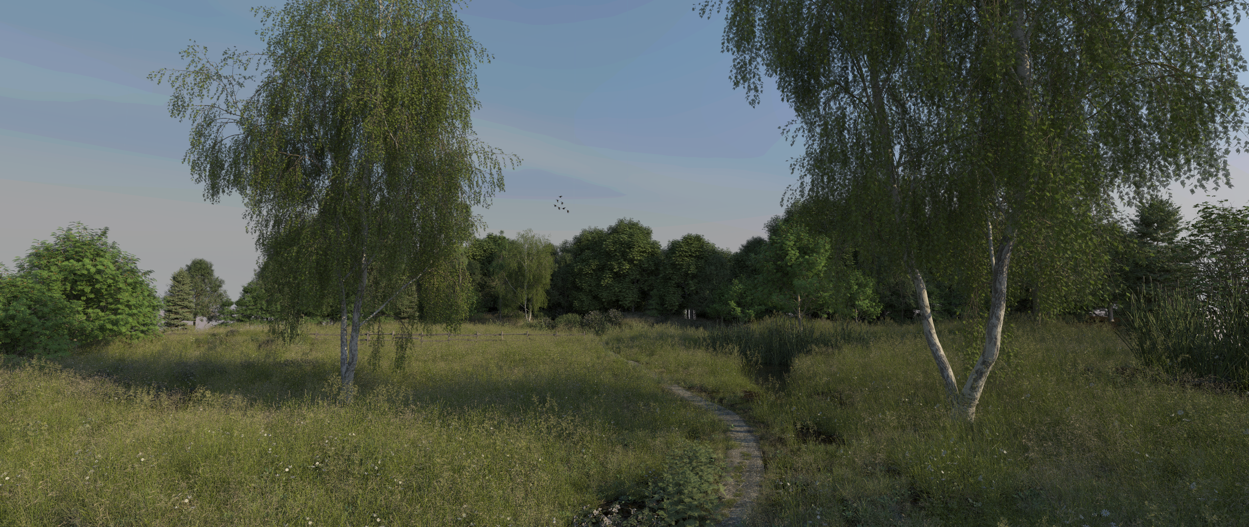
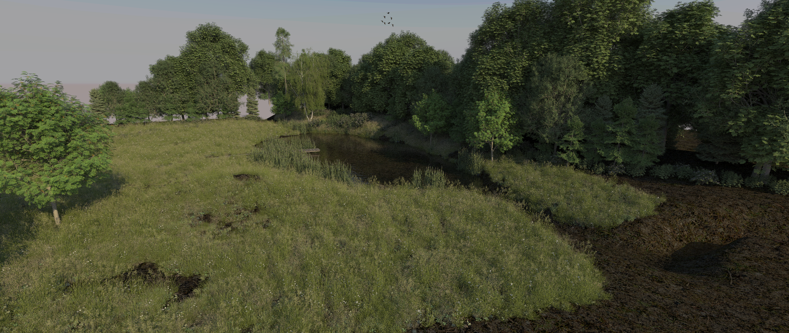
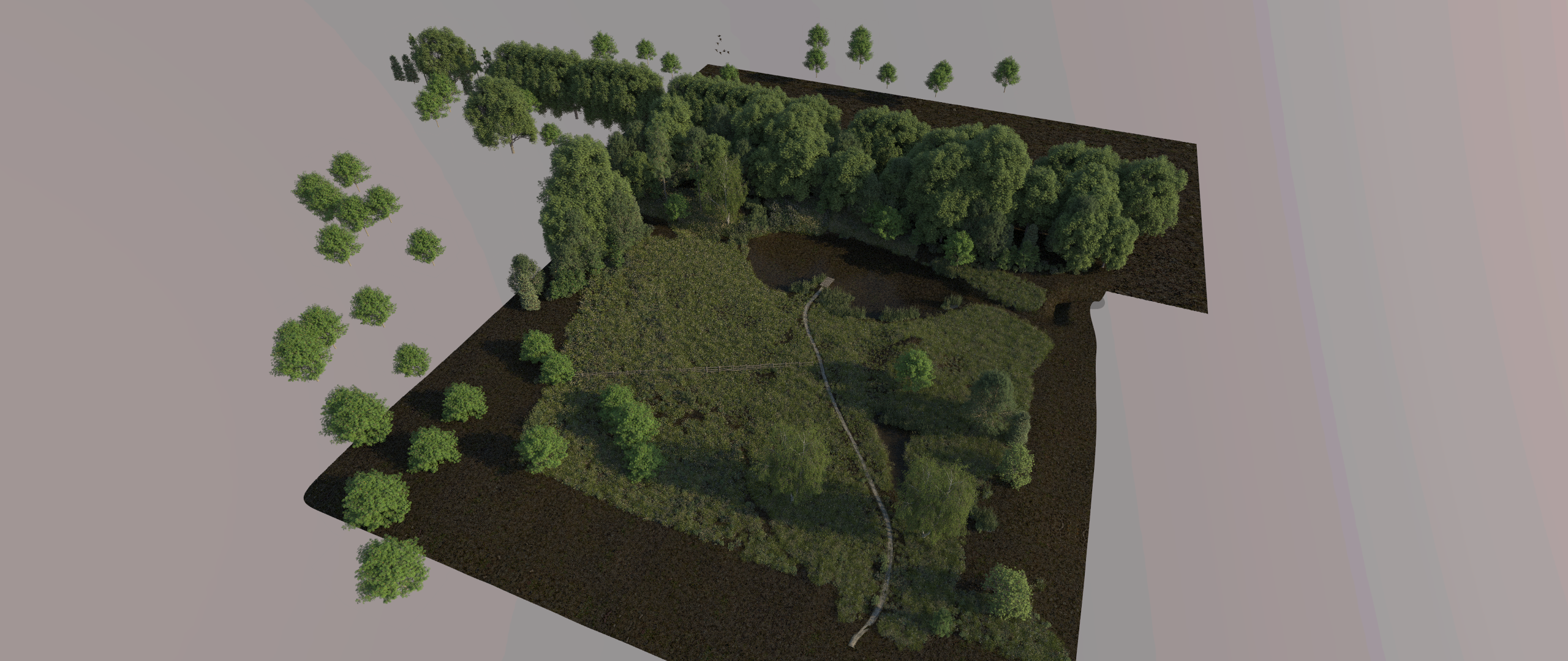
landscape model:  max GPU memory usage (on 8 ranks, including non-model data like ray queues, frame buffers, etc.) 3.7 GB (ours) vs 4.8 GB (spatial)
path: 6.1 fps (ours)  5.2 fps (spatial)	view-3: 9.1 fps (ours)  4.7 fps (spatial)	top: 13.3 fps (ours)  10.1 fps (spatial)
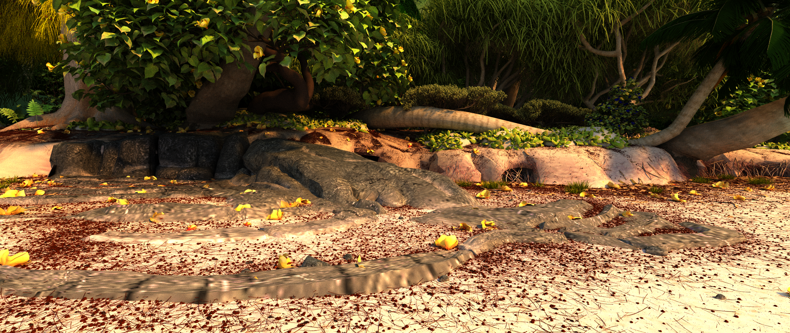
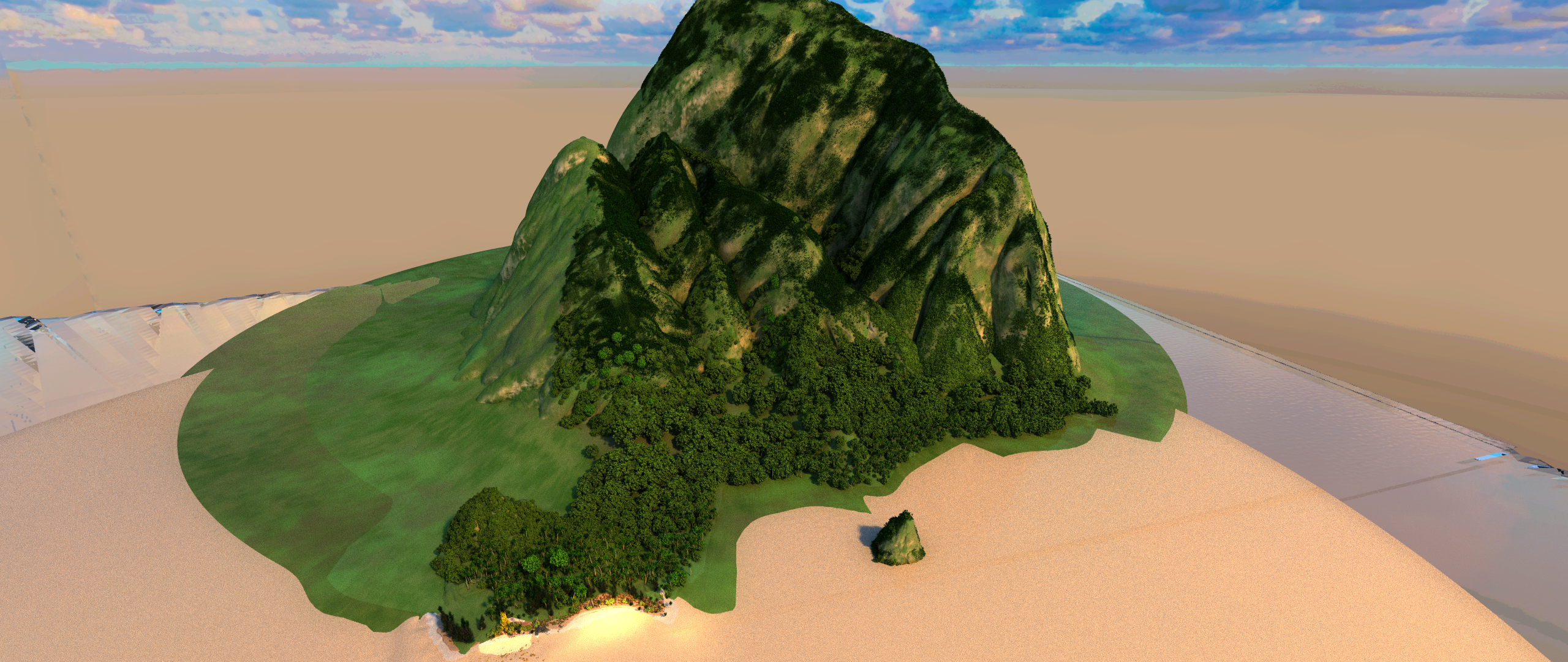
island model:  max GPU memory usage (on 8 ranks, including non-model data like ray queues, frame buffers, etc.): 25 GB (ours) vs 48 GB (spatial)
default: 7.9 fps (ours)  (3.0$\star$) fps (spatial)	beach: 3.6 fps (ours)  (2.8$\star$) fps (spatial)	overview: 11.1 fps (ours)  (3.7$\star$) fps (spatial)

Figure 4. Views used for our evaluation, and render performance for these views. ($2560\times 1080$, one path/pixel, 4 workers@$2\times$RTX 8000, 10-GigE Ethernet).
(^$\star$: spatial can render this model only if we upgrade the first rank to 128 GBs of RAM, and even then requires significant swapping during scene setup)

5. Implementation

The core contribution of this paper is not any one implementation, but the general concepts of looking beyond purely spatial partitioning, the proxies, and the specific techniques for the data-distributed traversal operating on these proxies. Nevertheless, to prove that these concepts do in fact work we also developed a data-distributed GPU path tracer that uses these concepts.

For communication we use a CUDA-aware build of OpenMPI 4.1.2, which means that we can directly pass device addresses to MPI, which then copies data as required. With better hardware this would also allow RDMA communication between GPUs and network devices, but on our low-end setup this is not the case. The renderer uses a wavefront-design, with all shading, compaction, etc., done in CUDA 11.4, and all tracing done using OptiX 7.4.

That same renderer can also be recompiled to a CPU-only version that uses Embree and TBB. The same concepts work there as well, but for our model the texturing in particular is an issue on that setup. A detailed comparison is beyond the scope of this paper.

5.1. Rays, Paths, Hits, and Ownership Masks

Our framework builds on small, self-contained path nodes that can be forwarded across the network. Each path contains a ray origin and direction, a throughput value [Boksansky and Marrs, 2021], and the pixel ID to which it belongs, plus some bits to indicate whether a ray is a shadow ray, in medium, etc. To track already visited nodes we use a bit-field of either 8 or 64 bits depending on number of ranks; for more ranks we would use the technique described in Section 3.3.7. We use half precision for ray direction and throughput, and encode all bits and pixel ID in a 32-bit integer.

For the currently closest intersection we only store the distance in ray.tmax, plus the node mask of the geometry that was hit. This means paths have to be re-traced for shading, but this is cheaper than sending hit information across the network. We could also have stored the node ID that produced the hit; but using a node mask is better: if the ray were to need forwarding and later terminates on another node, having the node mask of the hit allows this other rank to check if it, too, happens to have that data, thus allowing the ray to be shaded there without it having to be sent back.

Using this encoding, the path struct is a mere 36 bytes in size. We refer to that same structure as either ray or a path depending on context, but always mean that same struct. Paths always get generated and shaded in wavefronts; between two such shading operations each wavefront goes through a distributed traversal until every path is on the node it can be shaded on.

5.2. Distributed Path Tracing

For the forwarding logic we use an OptiX acceleration structure built over the proxies, with an intersection program that rejects all proxies whose ownership mask lists any node that the ray has already been on. If any next proxy was found we use its bit-mask to pseudo-randomly pick one of the ranks listed in that mask. Otherwise, the ray is done traversing, and can go to shading. In that case we check if that ray can be shaded on the current node, and if not, pseudo-randomly pick one of the ranks listed in its hit mask.

5.2.1. Wavefront Ray Traversal.

Our core operation is to take one wavefront of rays, and trace these—across nodes—until each ray has terminated traversal, and is on a node where it can be shaded. We call this the distributed ray traversal, and it proceeds in three stages: We first launch an OptiX program that traces each ray into the rank’s local geometry. This uses an anyhit program to do alpha texturing, and a closest hit program that updates the ray’s tmax and hit mask if a closer intersection is found. The program then updates the ray’s alreadyVisited mask, traces it into the proxy acceleration structure, and determines which rank that ray needs to be sent to next as described above. We then run a CUDA compaction kernel that rearranges all rays such that those that can be shaded locally go to one place, and those that need forwarding go to another, with the latter sorted by the rank they need to go to.

Once the rays are thus arranged all ranks collaboratively execute an MPI Allgetherv to exchange how many rays each rank wants to send to any other node, followed by an MPI All2all that moves the rays to their respective destinations. These three stages get repeated until no more rays need exchanging, at which point every rank has a wavefront of rays ready to be shaded on that rank.

5.2.2. Wavefront Shading and Secondary Ray Generation

After a wavefront has been traced to completion each rank locally shades its rays. Shadow rays that terminated traversal on the current rank check if that shadow ray did find an occluder, and if so, get discarded; those that didn’t atomically add their throughput value into the rank’s frame buffer. For non-shadow rays, those that did not find an intersection get shaded by either background or environment light, and get accumulated into the frame buffer.

For a non-shadow ray that did have a hit we first re-trace that ray into the local geometry to re-compute the full hit and BRDF data (Section 5.1). We sample the BRDF to produce either a reflected or refracted ray, modify the ray’s throughput value according to the sampled BRDF, and use rejection sampling to avoid tracing rays with too low a throughput value. The secondary ray—if not rejected—gets appended to the next step’s wavefront queue.

Shading can also generate a shadow ray. To prevent possibly unlimited growth of the ray queues we use repeated reservoir sampling [Wyman, 2021] and importance sampling to always choose at most one sample from possibly multiple different lights and light types. Thus any pixel can have at most two rays active at any time: one for the path itself, and one for its corresponding shadow ray. Shadow rays first compute the pixel contribution they would have if not occluded, then store that value in their throughput field, and set a bit in the path that flags this as a shadow ray.

5.2.3. Proxy-Guided Primary Ray Generation.

For primary rays we use the technique described in Section 3.3.6: each rank generates every primary ray and traces it into the proxy acceleration structure (which on modern hardware is very cheap). This ray then picks a primary owner based on the bits of the closest proxy, and all but one rank will then discard this ray. For rays that hit proxies stored on more than one rank we use the pixel ID as a tie-breaker, which in the pseudo-color images in Figure 4 can be observed as an checkerboard pattern on those objects that the partitioner chose to replicate. This is intentional, and allows the work to get shared by all the nodes that have the data.

5.3. Merging Ranks’ Partial Frame Buffers

Irrespective of which rank a path was generated on, it—and the secondary rays it may spawn—can terminate on any other node; so, every pixel can get contributed to by any rank. One way to handle that is to send every shading contributions back to the rank that generated the path; but that is expensive. Instead, we have each rank maintain a full frame buffer for all the image contributions computed on that rank. These partial-sum frame buffers eventually need to get added for the final image. For this we use what in visualization is known as parallel direct send compositing [Grosset et al., 2017]: each rank is responsible for one part of the final frame buffer, and gets other ranks’ contributions from those ranks. Each rank then adds up the parts it received, performs tone mapping, and sends the final RGBA pixels to the master.

6. Evaluation

Using the implementation described in the previous sections we can now evaluate how well these techniques work. Since this is the only large production content that is publicly available we focus primarily on the island model, but also include the PBRT landscape for reference. For island we enable the isMountainA/xgLowGrowth, and tessellate all curves geometry into 3 linear segments per curve segment. For the original model’s PTex textures [Burley and Lacewell, 2008] we perform a baking step that creates a per-mesh texture with $8\times 8$ texels per quad, with properly created texture coordinates added to each vertex.

For hardware we use what is called “Beowulf” cluster of, in our case, five similar networked PCs, using one as head node, and four as workers. Each worker is equipped with 64 GBs of RAM, and with two 48 GB RTX 8000 cards; the master only runs the display. For networking we use a commodity at-home 10Gig-E Ethernet, which is well below what modern data center hardware can provide (e.g., a Mellanox ConnectX-7 is rated at 400 GBit/s, vs our 10 GBit/s). Better interconnects also allow RDMA transfers, which our setup does not. Using such low-end network may look counter-intuitive, but is useful to establish a baseline, and forces us to always focus on the main problem: bandwidth.

6.1. Maximum GPU Memory Usage

The ultimate rationale behind data-parallel rendering is to reduce the amount of data per node until it fits per-node memory. As such, we first evaluated how well different partitioning strategies performed in reducing per-rank memory. To do this we took the island model, split it into a varying number of $N$ parts (from $N=1..128$), and logged the size of the respectively largest part—which is the part that would most exceed the memory budget. To measure this we used the cost function described above; this doesn’t include rendering related data like ray queues, etc., and is an approximation even for model data; but is hardware agnostic and easy to compute.

The result of this experiment are plotted in Figure 5: for purely spatial partitioning the first few splitting planes hardly manage to reduce max part size at all, even when we use multiple candidate planes; and even after splitting into 16 parts has barely been reduced by $2\times$. When pre-splitting the single-instance root object into its constituent meshes as proposed by Zellmann et al. [2020] the situation markedly improves (red lines), but even then it takes a lot of partitions to significantly reduce model size. For object partitioning max model size drops rapidly, and even with only 4 parts is almost as good as spatial partition is with 16; it also and eventually reaches a minimum that spatial partitioning cannot reach.

For our renderer that means that the object-space and hybrid partitionings will easily fit on the 8 GPUs we got for this experiment, and even for island only require 25 GBs out of the 48 GBs available. For the spatial partitions even with pre-splitting some of the GPUs will temporarily exceed their memory during acceleration structure build, which we currently allow by using CUDA managed memory to temporarily allow paging out of data while the scene is built.

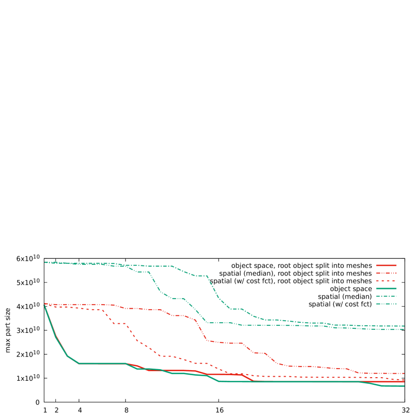
Figure 5. Estimated memory usage of the largest part when splitting island into any number from 1 to 32 parts, for different partitioning strategies; once with all non-instanced geometry together in one instance (green), and once with non-instanced objects broken into meshes (red).

6.2. Ray-Bandwidth Per Frame

The promise of our motivational example from Section 3.2 was that our techniques would not only help with how effectively a scene could be partitioned, but would ultimately even reduce ray bandwidth. To evaluate this we instrumented our MPI code to track, across all nodes and ray exchanges, how many such ray forwards were required to render a given frame. In Table 1 we report these numbers for the configurations and viewpoints shown in Figures 3 and 4: Naïve object space partitions incurs ray bandwidth several times higher than spatial techniques, but the introduction of proxies can reduce that significantly. Our currently best partitioner—which by default is allowed to replicate up to 5% of the input geometries—can do even better, and eventually requires $2-35\times$ less ray bandwidth than our best spatial techniques.

In practice, this result is important, for two reasons: First, for a system limited by how many rays can be sent across the network any reduction in ray bandwidth directly translates into higher frame rate. For the default view of island, using the same hardware resources our best object-space technique renders at 7.9 frames per second vs only 3 fps for spatial; for the view that captures the whole model, these are 11.1 fps vs 3.7 fps, respectively. When using more than one sample per pixel these speedups are even higher, as the bandwidth required for adding the final frames becomes less relevant.

Second, we observe that since our object space techniques require less GPU memory per rank (25 GB vs 48+GB, see Section 6.1) we could actually have used fewer ranks for these, likely achieving yet higher performance with less resources. For example, for landscape frame rate for our object techniques goes from 6.2 fps to 7.1 fps when going from 4 workers to 2.

	spatial only				object				hybrid
	sp.median		cost fct		naive		proxies		bvh-like		best
	PBRT landscape
path	1.9M	$(4.4\times)$	1.6M	$(3.6\times)$	6.7M	$(15\times)$	16M	$(36\times)$	4.3M	$(9.7\times)$	.45M
view-3	2.4M	$(5.2\times)$	2.2M	$(4.8\times)$	5.6M	$(12\times)$	33M	$(72\times)$	5.0M	$(11\times)$	.46M
top	.89M	$(7.6\times)$	1.5M	$(13\times)$	1.7M	$(14\times)$	7.3M	$(62\times)$	1.5M	$(13\times)$	.12M
	Moana island
default	5.0M	$(3.8\times)$	8.0M	$(6.2\times)$	19M	$(15\times)$	7.4M	$(5.7\times)$	9.7M	$(7.5\times)$	1.3M
beach	4.7M	$(1.7\times)$	7.3M	$(2.7\times)$	24M	$(8.7\times)$	14M	$(5.0\times)$	20M	$(7.4\times)$	2.7M
top	8.6M	$(43\times)$	7.3M	$(36\times)$	12M	$(59\times)$	6.9M	$(35\times)$	6.1M	$(31\times)$	.2M

Table 1. Rays forwarded across all nodes and bounces, for one path per pixel at $2560\times 1080$, using the given view and partitioning method (see Figures 3 and 4 for reference).

6.3. Application to Non-Instanced Models

To ascertain that our method is not limited to heavily instanced models we also developed a separate content pipeline that can handle large non-instanced models in an out of core fashion, creating the same spatial partitioning that existing data parallel renderers (e.g., in sci-vis) would produce. This works just fine; however, a full discussion of this is beyond the scope of this paper.

7. Summary and Discussion

In this paper, we have proposed a new approach to data parallel rendering that is more general than spatial partitioning; while simultaneously leading to better results in all of memory use, bandwidth, and performance. The downside of this generality is that it does not automatically define what the “best” partitioning might be, nor even a good heuristic for measuring the quality of a given partition, or for predicting the ray bandwidth required by one. Fully understanding this will require more research.

Our prototype renderer is, to our knowledge, the first to successfully demonstrate interactive yet data parallel path tracing on models of that kind that uses ray forwarding (even for spatial partitioning); however, real production renderers are more complex than ours, and moving these techniques into practice will require significant engineering. This is also true once we start using hardware with higher network bandwidth; this will require significant systems engineering to overlap communication with rendering, etc. We also can not yet handle techniques like bi-directional path tracing, photon mapping, or multiple importance sampling; some of this will require more work. Finally, it would be interesting to back-port some of our techniques into sci-vis, too; e.g., by using proxies on top of natively distributed sci-vis content.

8. Conclusion

The methods described in this paper allow for a more general description of how models can be represented in a data-parallel context, and when integrated into a non-trivial path tracer are not only more general, but can also achieve—simultaneously—lower memory use, lower ray bandwidth, and higher performance. Integrating these techniques into actual products will certainly require more research and more engineering work; however, we do believe that these techniques will significantly influence how future data parallel path tracers will be built.

References

- [1]
- Abram et al. [2018] G Abram, P Navratil, Pascal Grossett, D Rogers, and J Ahrens. 2018. Galaxy: Asynchronous Ray Tracing for Large High-Fidelity Visualization. In IEEE 8th Symposium on Large Data Analysis and Visualization (LDAV).
- Ahrens et al. [2005] James Ahrens, Berk Geveci, and Charles Law. 2005. Paraview: An end-user tool for large data visualization. The visualization handbook 717, 8 (2005).
- Benthin et al. [2017] Carsten Benthin, Sven Woop, Ingo Wald, and Attila Afra. 2017. Improved two-level BVHs using partial re-braiding. In Proceedings of High Performance Graphics.
- Boksansky and Marrs [2021] Jakub Boksansky and Adam Marrs. 2021. The Reference Path Tracer. In Ray Tracing Gems II - Next-Generation Real-Time Rendering with DXR, Vulkan, and OptiX, Adam Marrs, Peter Shirley, and Ingo Wald (Eds.). APress, Chapter 14.
- Burgess [2020] John Burgess. 2020. RTX ON–The NVIDIA Turing GPU. IEEE Micro 40, 2 (2020).
- Burley et al. [2018] Brent Burley, David Adler, Matt Jen-Yuan Chiang, Hank Driskill, Ralf Habel, Patrick Kelly, Peter Kutz, Yining Karl Li, and Daniel Teece. 2018. The Design and Evolution of Disney’s Hyperion Renderer. ACM Transactions on Graphics (TOG) (2018).
- Burley and Lacewell [2008] Brent Burley and Dylan Lacewell. 2008. Ptex: Per-Face Texture Mapping for Production Rendering. In Eurographics Symposium on Rendering 2008.
- Childs et al. [2012] H Childs, E Brugger, B Whitlock, J Meredith, S Ahern, D Pugmire, K Biagas, M Miller, C Harrison, GH Weber, H Krishnan, T Fogal, A Sanderson, C Garth, E Wes Bethel, D Camp, O Rübel, M Durant, JM Favre, and P Navratil. 2012. VisIt: An End-User Tool For Visualizing and Analyzing Very Large Data. In High Performance Visualization-Enabling Extreme-Scale Scientific Insight.
- DeMarle et al. [2004] David E DeMarle, Christiaan Gribble, and Steven G Parker. 2004. Memory-Savvy Distributed Interactive Ray Tracing. In 5th Eurographics/ACM SIGGRAPH Symposium on Parallel Graphics and Visualization (EGPGV 2004).
- Ernst and Greiner [2007] Manfred Ernst and Guenther Greiner. 2007. Early Split Clipping for Bounding Volume Hierarchies. In IEEE Symposium on Interactive Ray Tracing.
- Ganestam and Doggett [2016] Per Ganestam and Michael Doggett. 2016. SAH guided spatial split partitioning for fast BVH construction. In Rendering Techniques.
- Gropp et al. [1999] William Gropp, William D Gropp, Ewing Lusk, Anthony Skjellum, and Argonne Distinguished Fellow Emeritus Ewing Lusk. 1999. Using MPI: portable parallel programming with the message-passing interface. Vol. 1.
- Grosset et al. [2017] P Grosset, M Prasad, C Christensen, A Knoll, and C Hansen. 2017. TOD-Tree: Task-Overlapped Direct Send Tree Image Compositing for Hybrid MPI Parallelism and GPUs. IEEE Transactions on Visualization and Computer Graphics 23, 6 (2017).
- Hapala et al. [2011] Michal Hapala, Tomas Davidovic, Ingo Wald, Vlastimil Havran, and Philipp Slusallek. 2011. Efficient stack-less BVH traversal for ray tracing. In SCCG ’11: Proceedings of the 27th Spring Conference on Computer Graphics.
- Ize et al. [2011] Thiago Ize, Carson Brownle, and Charles D Hansen. 2011. Real-Time Ray Tracer for Visualizing Massive Models on a Cluster. In Eurographics Symposium on Parallel Graphics and Visualization.
- Jaros et al. [2021] Milan Jaros, Lubomir Riha, Petr Strakos, and Matej Spetko. 2021. GPU Accelerated Path Tracing of Massive Scenes. ACM Transaction on Graphics 40, 2 (2021).
- Karras and Aila [2013] Tero Karras and Timo Aila. 2013. Fast Parallel Construction of High-quality Bounding Volume Hierarchies. In High-Performance Graphics Conference.
- Kato and Saito [2002] Toshi Kato and Jun Saito. 2002. “Kilauea” – Parallel Global Illumination Renderer. In Fourth Eurographics Workshop on Parallel Graphics and Visualization.
- Moreland [2011] Kenneth Moreland. 2011. IceT Users’ Guide and Reference. Technical Report. Sandia National Labs.
- Park et al. [2018] Hyungman Park, Donald Fussell, and Paul Navratil. 2018. SpRay: Speculative Ray Scheduling for Large Data Visualization. In IEEE Symposium on Large Data Analysis and Visualization.
- Parker et al. [2010] Steven G Parker, James Bigler, Andreas Dietrich, Heiko Friedrich, Jared Hoberock, David Luebke, David McAllister, Morgan McGuire, Keith Morley, Austin Robison, et al. 2010. Optix: A General Purpose Ray Tracing Engine. Acm transactions on graphics (tog) 29, 4 (2010), 1–13.
- Pharr et al. [1997] Matt Pharr, Craig Kolb, Reid Gershbein, and Pat Hanrahan. 1997. Rendering complex scenes with memory-coherent ray tracing. In SIGGRAPH ’97: Proceedings of the 24th annual conference on Computer graphics and interactive techniques.
- Reinhard [1995] Erik Reinhard. 1995. Scheduling and Data Management for Parallel Ray Tracing. Ph.D. Dissertation. University of East Anglia.
- Salmon and Goldsmith [1989] J. Salmon and J. Goldsmith. 1989. A Hypercube Ray-Tracer. In C3P: Proceedings of the third conference on Hypercube concurrent computers and applications - Volume 2.
- Stich et al. [2009] Martin Stich, Heiko Friedrich, and Andreas Dietrich. 2009. Spatial Splits in Bounding Volume Hierarchies. In HPG ’09: Proceedings of the Conference on High Performance Graphics 2009.
- Vaidyanathan et al. [2019] Karthik Vaidyanathan, Sven Woop, and Carsten Benthin. 2019. Wide BVH Traversal with a Short Stack. In High-Performance Graphics - Short Papers.
- Wald et al. [2020] Ingo Wald, Bruce Cherniak, Will Usher, Carson Brownlee, Attila T. Áfra, Johannes Günther, Jefferson Amstutz, Tim Rowley, Valerio Pascucci, Chris R. Johnson, and Jim Jeffers. 2020. Digesting the Elephant - Experiences with Interactive Production Quality Path Tracing of the Moana Island Scene. http://arxiv.org/abs/2001.02620 arXiv 2001.02620.
- Wald et al. [2001] Ingo Wald, Philipp Slusallek, and Carsten Benthin. 2001. Interactive Distributed Ray Tracing of Highly Complex Models. In Eurographics Workshop on Rendering Techniques.
- Wald et al. [2014] Ingo Wald, Sven Woop, Carsten Benthin, Gregory S Johnson, and Manfred Ernst. 2014. Embree: A Kernel Framework for efficient CPU Ray Tracing. ACM Transactions on Graphics (TOG) 33, 4 (2014), 1–8.
- Walker and Dongarra [1996] David W Walker and Jack J Dongarra. 1996. MPI: a standard message passing interface. Supercomputer 12 (1996).
- Wyman [2021] Chris Wyman. 2021. Weighted Reservoir Sampling: Randomly Sampling Streams. In Ray Tracing Gems II - Next-Generation Real-Time Rendering with DXR, Vulkan, and OptiX, Adam Marrs, Peter Shirley, and Ingo Wald (Eds.). APress, Chapter 20.
- Xie et al. [2021] Feng Xie, Petro Mishchuk, and Warren Hunt. 2021. Real Time Cluster Path Tracing. In SIGGRAPH Asia 2021 Technical Communications.
- Zellmann et al. [2020] Stefan Zellmann, Nathan Morrical, Ingo Wald, and Valerio Pascucci. 2020. Finding Efficient Spatial Distributions for Massively Instanced 3-d Models. In EGPGV Eurographics/EuroVis.