Light Deflection by Rotating Regular Black Holes with a Cosmological Constant

Abstract

Using the Gauss-Bonnet theorem, we compute and examine the deflection angle of light rays by rotating regular black holes with a cosmological constant. By the help of optical geometries, we first deal with the Hayward black holes with cosmological contributions. Then, we reconsider the study of the Bardeen solutions. We inspect the cosmological constant effect on the deflection angle of light rays. Concretely, we find extra cosmological correction terms generalizing certain obtained findings. Using graphical analysis, we provide a comparative discussion with respect to the Kerr solutions. The results confirm that the non-linear electrodynamic charges affect the space-time geometry by decreasing the deflection angle of light rays by such cosmological black holes.

Keywords: Regular black holes, Deflection angle formalism, Gauss-Bonnet theorem, Cosmological constant.

1 Introduction

Black hole physics has received a remarkable interest due to recent detections and observational findings supporting the obtained theoretical investigations. Precisely, Even Horizon Telescope (EHT) has provided an image of a black hole [1, 2, 3, 4]. This discovery has been followed by significant efforts reserved to the investigation of various black hole aspects [5, 6]. These involve the thermodynamics and the optical behaviors encoding many interesting data of the associated physics. In connections with Anti de Sitter geometries, the thermodynamic quantities have been approached by linking the cosmological constant with the pressure [7, 8, 9, 10]. Based on such an interplay, certain phase transitions, including the Hawking-Page one, have been dealt with extensively in many places including in [11]. It has been observed many similarities with fluid physical systems [12, 13]. Besides that, optical properties of the black holes have been also studied by focusing on two relevant notions, being the shadow and the deflection angle of light rays. The first concept has been discussed in terms of one dimensional real curves [14, 15, 16, 17]. In this way, the corresponding size and shape have been controlled by the involved black hole parameters [18, 19, 20, 21, 22]. The second notion concerns the deflection angle of light rays by black holes which has been investigated using different methods[23, 24, 25, 26, 27]. A priori, there are two famous ones. One is relied on an elliptic formalism involving non-trivial elliptic functions including the hypergeometric ones, explored to compute the so-called total deflection angle[28, 29]. The second method, which will be exploited here, is based on the Gauss-Bonnet theorem results [30, 31, 32]. Precisely, Gibbons and Werner suggested a nice road to compute the deflection angle of light rays by black holes [33]. In this regard, many models have been discussed including regular black hole geometries [34]. These solutions have been interpreted in terms of gravitational backgrounds with non-linear electromagnetic charges. The key interest on these black holes comes from the understanding of certain singularities thanks to the pioneer works of Penrose and Hawking [35, 36]. Then, Bardeen discovered a regular black hole obeying the weak energy condition. After that, many Bardeen-like black hole solutions have been investigated where the irregularity has been linked to topological changes. This has been exploited to provide a possibility to build spaces with a maximum curvature inside the black holes [37, 38]. Moreover, other regular black hole models have been suggested by coupling the Einstein’s theory with nonlinear electrodynamics [39]. It has been shown that the regular black hole interior solutions have been found in many gravity models like Loop Quantum Gravity [40]. The black hole solutions of Bardeen and Hayward have been extensively studied by examining either thermodynamics properties or shadow optical ones [41, 42].

The aim of this work is to contribute to such activities by investigating the deflection angle of light rays by regular black holes with a cosmological constant. Using the techniques explored in [30, 31, 32], we compute and examine such an optical quantity of the rotating Hayward regular black holes and Bardeen regular black holes in terms of existing parameters. Taking the finite distance contributions, we inspect the effect of such parameters. A particular emphasis puts on the cosmological constant influence. Then, we provide a comparison study with respect to the Kerr solutions with negative and positive cosmological constant values. This finding confirms that the non-linear electrodynamic charges affect the space-time geometry by decreasing the deflection angle of light rays near such black holes with a cosmological constant.

This paper is organized as follows. In section 2, we present the formalism needed to compute the deflection angle of light rays. In section 2, we consider the rotating regular Hayward black hole with a cosmological constant. In section 4, we deal with the rotating regular Bardeen black holes with cosmological contributions. In section 5, we provide a comparative study by elaborating graphical analysis using results of the Kerr solutions. The last section concerns concluding remarks.

2 Deflection angle formalism

In this section, we give a concise review on the computations of the light deflection angle around a black hole. An examination shows that various methods have been proposed and exploited for many solutions. The known one has been based on the Gauss-Bonnet theorem results being extensively used to approach several black hole backgrounds [30]. In the present work, we will exploit these findings to examine such an optical quantity where the observer and the source are placed at finite distances. In particular, the calculations relay on the method developed in [31]. In this way, the deflection angle of light rays can be expressed via the relation

$$\Theta=\Psi_{R}-\Psi_{S}+\phi_{SR}$$ (2.1)

where $\Psi_{R}$ and $\Psi_{S}$ are the angles between the light rays and the radial direction at the observer and the source position, respectively. It is denoted that $\phi_{SR}$ is the longitude separation angle, which will be specified later on[30]. To write down the associated formula, an unit tangential vector along the light will be used. This vector denoted $e^{i}$ is linked to the above angle as follows

$$(e^{r},e^{\theta},e^{\phi})=\epsilon\left(\frac{dr}{d\phi},0,1\right)$$ (2.2)

where $\epsilon$ is a radial quantity which can be determined from the metric black hole solutions. Putting such a metric as follows

$$ds^{2}=-A(r,\theta)dt^{2}+B(r,\theta)dr^{2}+C(r,\theta)d\theta^{2}+D(r,\theta)d\phi^{2}-2H(r,\theta)dtd\phi,$$ (2.3)

it is possible to get its expression. Concretely, it is given by

$$\epsilon=\frac{A(r)D(r)+H^{2}(r)}{A(r)(H(r)+A(r)b)}$$ (2.4)

where $b$ is the impact parameter considered as a ratio of the two constants of motion derived from the orbit equation. A simplified form can be determined by considering the equatorial plane. Indeed, these two conserved quantities read as

$$E=A(r)\dot{t}+H(r)\dot{\phi}\qquad L=D(r)\dot{\phi}-H(r)\dot{t}$$ (2.5)

where the derivative with respect to the affine parameter has been used. They represent the energy and the angular momentum of the test particle, respectively. Considering a constant $t$ of the space-time metric, a 2-dimensional curved space can be built being relevant in the calculations of the light deflection angle. In the equatorial plane, its element line should take the following form

$$dl^{2}\equiv\gamma_{ij}dx^{i}dx^{j}$$ (2.6)

where $\gamma_{ij}$ is a spatial metric encoding the involved physical parameters. In this space, the deflection angle of light rays can be measured from the radial direction. The above angle can be determined by taking the particular angle $\theta=\frac{\pi}{2}$ and using the relation

$$\cos\Psi\equiv\gamma_{ij}e^{i}R^{j},$$ (2.7)

where $R^{j}$ are the components of a radial vector given by $(\frac{1}{\sqrt{\gamma_{rr}}},0,0)$. Exploiting Eq.(2.2) and Eq.(2.7), the $\sin\Psi$ term can be obtained from the following relation

$$\sin\Psi=\frac{H(r)+A(r)b}{\sqrt{A(r)D(r)+H^{2}(r)}}.$$ (2.8)

With this formalism in hand, we can calculate the deflection angle of light rays by rotating regular black holes in cosmological backgrounds by considering the retrograde situation. This will be the aim of the forthcoming sections. In particular, we consider two models followed by a comparative discussion.

3 Deflection angle of light rays by cosmological Hayward black hole solutions

In this section, we investigate the deflection angle of light rays around the rotating Hayward black holes with a cosmological constant. As mentioned before, the calculations are based on the metric form. In the Boyer-Lindquist coordinates, this is given via the following line element

$$ds^{2}=-\frac{\Delta_{r}}{\Sigma}\left(dt-\frac{a\sin^{2}\theta}{\Xi}d\phi\right)^{2}+\frac{\Sigma}{\Delta_{r}}dr^{2}+\frac{\Sigma}{\Delta_{\theta}}d\theta^{2}+\frac{\Delta_{\theta}\sin^{2}\theta}{\Sigma}\left(adt-\frac{r^{2}+a^{2}}{\Xi}d\phi\right)^{2}.$$ (3.1)

The physical terms appearing in such a metric can be expressed as follows

$$\Delta_{r} = \left(r^{2}+a^{2}\right)\left(1-\frac{r^{2}\Lambda}{3}\right)-2M\left(\frac{r^{3}}{r^{3}+g_{h}^{3}}\right)r,\hskip 28.45274pt\Delta_{\theta}=1+\frac{a^{2}\Lambda}{3}\cos^{2}\theta,$$ (3.2)

$$\Xi = 1+\frac{a^{2}\Lambda}{3},\hskip 28.45274pt\Sigma=r^{2}+a^{2}\cos^{2}\theta.$$ (3.3)

Here, $M$ and $a$ represent the mass and the rotating parameter, respectively. $g_{h}$ indicates the charge of the non-linear electrodynamics and $\Lambda$ is the cosmological constant. Using the impact parameter given by $b=\frac{L}{E}$ and changing the variable $r$ to $\frac{1}{u}$, we can get

$$\left(\frac{du}{d\phi}\right)^{2} = \frac{1}{b^{2}}-\frac{4aMu}{b^{3}}-u^{2}+2Mu^{3}+\frac{\Lambda}{3}-\frac{2a\Lambda}{3b^{3}u^{2}}-\frac{8a\Lambda M}{3b^{3}u}+\frac{4aMu^{4}g_{h}^{3}}{b^{3}}-2Mu^{6}g_{h}^{3}$$ (3.4)

$$+ \frac{8a\Lambda Mu^{2}g_{h}^{3}}{3b^{3}}+\mathcal{O}({M^{2},\Lambda^{2},a^{2},g_{h}^{4}}),$$

where one has considered only the retrograde solution. In the beginning, one should calculate the separation angle integral. Putting $\left(\frac{du}{d\phi}\right)^{2}=F(u)$, this can be determined via the following computation

$$\phi_{RS}=\int^{R}_{S}d\phi=\int^{u_{0}}_{u_{S}}\frac{1}{\sqrt{F(u)}}du+\int^{u_{0}}_{u_{R}}\frac{1}{\sqrt{F(u)}}du,$$ (3.5)

where $u_{S}$ and $u_{R}$ are the inverse of the source and the observer distance from the black hole and where $u_{0}$ is the inverse of the closest approach $r_{0}$. Considering the weak field and the slow rotation approximations, the impact parameter can be related to $u_{0}$ as follows

$$b=\frac{1}{u_{0}}+M-2aMu_{0}+\mathcal{O}({M^{2},\Lambda,a^{2},g_{h}}).$$ (3.6)

Performing appropriate calculations, we obtain

$$\phi_{RS} = \phi_{RS}^{Kerr}+\left(\frac{u_{R}\left(2b^{4}u_{R}^{4}+5b^{2}u_{R}^{2}-15\right)}{\sqrt{1-b^{2}u_{R}^{2}}}+\frac{u_{S}\left(2b^{4}u_{S}^{4}+5b^{2}u_{S}^{2}-15\right)}{\sqrt{1-b^{2}u_{S}^{2}}}\right)\frac{Mg_{h}^{3}}{8b^{3}}$$ (3.7)

$$+ \left(\frac{u_{R}\left(b^{2}u_{R}^{2}-3\right)}{\sqrt{1-b^{2}u_{R}^{2}}}+\frac{u_{S}\left(b^{2}u_{S}^{2}-3\right)}{\sqrt{1-b^{2}u_{S}^{2}}}\right)\frac{aMg_{h}^{3}}{b^{4}}$$

$$- \left(\frac{u_{R}\left(3b^{4}u_{R}^{4}-20b^{2}u_{R}^{2}+15\right)}{\left(1-b^{2}u_{R}^{2}\right){}^{3/2}}+\frac{u_{S}\left(3b^{4}u_{S}^{4}-20b^{2}u_{S}^{2}+15\right)}{\left(1-b^{2}u_{S}^{2}\right){}^{3/2}}\right)\frac{\Lambda Mg_{h}^{3}}{12b}$$

$$+ \left(\pi-\arcsin\left(bu_{R}\right)-\arcsin\left(bu_{S}\right)\right)\left(-\frac{15Mg_{h}^{3}}{8b^{4}}+\frac{3aMg_{h}^{3}}{b^{5}}-\frac{5\Lambda Mg_{h}^{3}}{4b^{2}}\right)$$

$$+ \left(\frac{u_{R}}{\sqrt{1-b^{2}u_{R}^{2}}}+\frac{u_{S}}{\sqrt{1-b^{2}u_{S}^{2}}}\right)\frac{b^{3}\Lambda}{6}+\left(\frac{b\left(2-3b^{2}u_{R}^{2}\right)}{2\left(1-b^{2}u_{R}^{2}\right){}^{3/2}}+\frac{b\left(2-3b^{2}u_{S}^{2}\right)}{2\left(1-b^{2}u_{S}^{2}\right){}^{3/2}}\right)\frac{M\Lambda}{3}$$

$$+ \left(\frac{1-2b^{2}u_{R}^{2}}{u_{R}\sqrt{1-b^{2}u_{R}^{2}}}+\frac{1-2b^{2}u_{S}^{2}}{u_{S}\sqrt{1-b^{2}u_{S}^{2}}}\right)\frac{a\Lambda}{3}+\mathcal{O}({M^{2},\Lambda^{2},a^{2},g_{h}^{4}},Ma\Lambda,Ma\Lambda g_{h}^{3}),$$

where the Kerr term is given by

$$\phi_{RS}^{Kerr} = \phi_{RS}^{SW}-\left(\frac{1}{\sqrt{1-b^{2}u_{R}^{2}}}+\frac{1}{\sqrt{1-b^{2}u_{S}^{2}}}\right)\frac{2aM}{b^{2}}.$$ (3.8)

In this equation, the Schwarzschild term is

$$\phi_{RS}^{SW}=\pi-\arcsin\left(bu_{R}\right)-\arcsin\left(bu_{S}\right)+\left(\frac{2-b^{2}u_{R}^{2}}{\sqrt{1-b^{2}u_{R}^{2}}}+\frac{2-b^{2}u_{S}^{2}}{\sqrt{1-b^{2}u_{S}^{2}}}\right)\frac{M}{b}.$$ (3.9)

To get the remaining terms appearing in the light deflection angle expression, one should identify the $\Psi$ terms. By using the Eq.(2.8), we find

$$\sin\Psi = bu-bMu^{2}+2aMu^{2}-\left(\frac{bM}{6}-\frac{a}{3u}+\frac{b}{6u}\right)\Lambda+\left(bu^{5}-2au^{5}+\frac{b\Lambda u^{3}}{6}\right)Mg_{h}^{3}$$ (3.10)

$$+ \mathcal{O}({M^{2},\Lambda^{2},a^{2},g_{h}^{4}},Ma\Lambda,Ma\Lambda g_{h}^{3}).$$

This relation produces

$$\Psi_{R} - \Psi_{S}=\Psi_{R}^{Kerr}-\Psi_{S}^{Kerr}+\left(\frac{bu_{R}^{5}}{\sqrt{1-b^{2}u_{R}^{2}}}+\frac{bu_{S}^{5}}{\sqrt{1-b^{2}u_{S}^{2}}}\right)Mg_{h}^{3}$$ (3.11)

$$- \left(\frac{u_{R}^{5}}{\sqrt{1-b^{2}u_{R}^{2}}}+\frac{u_{S}^{5}}{\sqrt{1-b^{2}u_{S}^{2}}}\right)2aMg_{h}^{3}-\left(\frac{u_{R}^{3}\left(2b^{2}u_{R}^{2}-1\right)}{\left(1-b^{2}u_{R}^{2}\right){}^{3/2}}+\frac{u_{S}^{3}\left(2b^{2}u_{S}^{2}-1\right)}{\left(1-b^{2}u_{S}^{2}\right){}^{3/2}}\right)\frac{b\Lambda Mg_{h}^{3}}{6}$$

$$- \left(\frac{1}{u_{R}\sqrt{1-b^{2}u_{R}^{2}}}+\frac{1}{u_{S}\sqrt{1-b^{2}u_{S}^{2}}}\right)\frac{b\Lambda}{6}-\left(\frac{2b^{2}u_{R}^{2}-1}{\left(1-b^{2}u_{R}^{2}\right){}^{3/2}}+\frac{2b^{2}u_{S}^{2}-1}{\left(1-b^{2}u_{S}^{2}\right){}^{3/2}}\right)\frac{b\Lambda M}{6}$$

$$+ \left(\frac{1}{u_{R}\sqrt{1-b^{2}u_{R}^{2}}}+\frac{1}{u_{S}\sqrt{1-b^{2}u_{S}^{2}}}\right)\frac{a\Lambda}{3}+\mathcal{O}({M^{2},\Lambda^{2},a^{2},g_{h}^{4}},Ma\Lambda,Ma\Lambda g_{h}^{3}),$$

where one has

$$\Psi_{R}^{Kerr} - \Psi_{S}^{Kerr}=\Psi_{R}^{SW}-\Psi_{S}^{SW}+\left(\frac{u_{R}^{2}}{\sqrt{1-b^{2}u_{R}^{2}}}+\frac{u_{S}^{2}}{\sqrt{1-b^{2}u_{S}^{2}}}\right)2aM,$$ (3.12)

and where one has found

$$\Psi_{R}^{SW}-\Psi_{S}^{SW}=\left(\arcsin\left(bu_{R}\right)+\arcsin\left(bu_{S}\right)-\pi\right)-\left(\frac{u_{R}^{2}}{\sqrt{1-b^{2}u_{R}^{2}}}+\frac{u_{S}^{2}}{\sqrt{1-b^{2}u_{S}^{2}}}\right)Mb.$$ (3.13)

Combining the above equations, we get an expression of the light deflection angle given by

$$\alpha_{h} = \left(\sqrt{1-b^{2}u_{R}^{2}}+\sqrt{1-b^{2}u_{S}^{2}}\right)\frac{2M}{b}-\left(\sqrt{1-b^{2}u_{R}^{2}}-\sqrt{1-b^{2}u_{S}^{2}}\right)\frac{2aM}{b^{2}}$$ (3.14)

$$- \left(\frac{1-b^{2}u_{R}^{2}}{u_{R}\sqrt{1-b^{2}u_{R}^{2}}}+\frac{1-b^{2}u_{S}^{2}}{u_{S}\sqrt{1-b^{2}u_{S}^{2}}}\right)\frac{\text{b$\Lambda$}}{6}+\left(\frac{1}{\sqrt{1-b^{2}u_{R}^{2}}}+\frac{1}{\sqrt{1-b^{2}u_{S}^{2}}}\right)\frac{b\Lambda M}{6}$$

$$+ \left(\frac{\sqrt{1-b^{2}u_{R}^{2}}}{u_{R}}+\frac{\sqrt{1-b^{2}u_{S}^{2}}}{u_{S}}\right)\frac{2a\Lambda}{3}+\left(\frac{u_{R}\left(2b^{4}u_{R}^{4}+b^{2}u_{R}^{2}-3\right)}{\sqrt{1-b^{2}u_{R}^{2}}}+\frac{u_{S}\left(2b^{4}u_{S}^{4}+b^{2}u_{S}^{2}-3\right)}{\sqrt{1-b^{2}u_{S}^{2}}}\right)\frac{5Mg_{h}^{3}}{8b^{3}}$$

$$- \left(\frac{u_{R}\left(2b^{4}u_{R}^{4}+b^{2}u_{R}^{2}-3\right)}{b^{4}\sqrt{1-b^{2}u_{R}^{2}}}+\frac{u_{S}\left(2b^{4}u_{S}^{4}+b^{2}u_{S}^{2}-3\right)}{b^{4}\sqrt{1-b^{2}u_{S}^{2}}}\right)\frac{aMg_{h}^{3}}{b^{4}}$$

$$+ \left(\frac{u_{R}\left(7b^{2}u_{R}^{2}-15\right)}{\sqrt{1-b^{2}u_{R}^{2}}}+\frac{u_{S}\left(7b^{2}u_{S}^{2}-15\right)}{\sqrt{1-b^{2}u_{S}^{2}}}\right)\frac{\Lambda Mg_{h}^{3}}{12b}$$

$$+ \left(\pi-\arcsin\left(bu_{R}\right)-\arcsin\left(bu_{S}\right)\right)\left(-\frac{15Mg_{h}^{3}}{8b^{4}}+\frac{3aMg_{h}^{3}}{b^{5}}-\frac{5\Lambda Mg_{h}^{3}}{4b^{2}}\right)$$

$$+ \mathcal{O}({M^{2},\Lambda^{2},a^{2},g_{h}^{4}},Ma\Lambda,Ma\Lambda g_{h}^{3}).$$

This form can be reduced to a simplified one using certain convenable approximations. Taking $u_{S}b<<1$ and $u_{R}b<<1$, we can get an expression involving divergent terms coupled to the cosmological contributions. These terms should be existed to show the cosmological background dependance. The desired deflection angle of light rays is found to be

$$\alpha_{h} = \frac{4M}{b}-\frac{4aM}{b^{2}}-\frac{15\pi Mg_{h}^{3}}{8b^{4}}+\frac{3\pi aMg_{h}^{3}}{b^{5}}-\frac{5\Lambda\text{$\pi$M}g_{h}^{3}}{4b^{2}}+\frac{b\Lambda M}{3}-\left(\frac{1}{u_{R}}+\frac{1}{u_{S}}\right)\frac{b\Lambda}{6}$$ (3.15)

$$+ \left(\frac{1}{u_{R}}+\frac{1}{u_{S}}\right)\frac{2a\Lambda}{3}+\mathcal{O}({M^{2},\Lambda^{2},a^{2},g_{h}^{4}},Ma\Lambda,Ma\Lambda g_{h}^{3}).$$

An examination shows that this expression recovers many previous findings. In the absence of the cosmological contributions, we get the results of the ordinary Hayward solutions investigated in [34]. Moreover, the Schwarzschild black hole and the Kerr black hole results can be obtained by sending the extra parameters to zero[43].

4 Deflection angle of light rays by cosmological Bardeen black holes

In this section, we deal with other regular black holes. Precisely, we study the deflection angle of light rays around the rotating Bardeen black holes with a cosmological constant. To start, we give the associated metric in the Boyer-Lindquist coordinates. In this way, the line element of such a metric reads as

$$ds^{2}=-\frac{\Delta_{r}}{\Sigma}\left(dt-\frac{a\sin^{2}\theta}{\Xi}d\phi\right)^{2}+\frac{\Sigma}{\Delta_{r}}dr^{2}+\frac{\Sigma}{\Delta_{\theta}}d\theta^{2}+\frac{\Delta_{\theta}\sin^{2}\theta}{\Sigma}\left(adt-\frac{r^{2}+a^{2}}{\Xi}d\phi\right)^{2}.$$ (4.1)

This involves the physical terms

$$\Delta_{r} = \left(r^{2}+a^{2}\right)\left(1-\frac{r^{2}\Lambda}{3}\right)-2M\left(\frac{r^{2}}{r^{2}+g_{b}^{2}}\right)^{\frac{3}{2}}r,\qquad\Delta_{\theta}=1+\frac{a^{2}\Lambda}{3}\cos^{2}\theta,$$ (4.2)

$$\Xi = 1+\frac{a^{2}\Lambda}{3},\qquad\Sigma=r^{2}+a^{2}\cos^{2}\theta$$

where $M$ and $a$ denote the mass and the rotating parameter of the black hole, respectively. $g_{b}$ represents the charge of the nonlinear electrodynamics. To compute the associated deflection angle, the orbit equation is needed being relevant as indicated in the previous section. A close examination provides the following relation

$$\left(\frac{du}{d\phi}\right)^{2} = \frac{1}{b^{2}}-\frac{4aMu}{b^{3}}-u^{2}+2Mu^{3}+\frac{\Lambda}{3}-\frac{2a\Lambda}{3b^{3}u^{2}}-\frac{8a\Lambda M}{3b^{3}u}-3Mu^{5}g_{b}^{2}$$ (4.3)

$$+ \frac{6aMu^{3}g_{b}^{2}}{b^{3}}+\frac{4a\Lambda Mug_{b}^{2}}{b^{3}}+\mathcal{O}({M^{2},\Lambda^{2},a^{2},g_{b}^{3}}).$$

After computations, we obtain

$$\phi_{RS} = \phi_{RS}^{Kerr}+\left(\frac{b^{4}u_{R}^{4}+4b^{2}u_{R}^{2}-8}{2b^{3}\sqrt{1-b^{2}u_{R}^{2}}}+\frac{b^{4}u_{S}^{4}+4b^{2}u_{S}^{2}-8}{2b^{3}\sqrt{1-b^{2}u_{S}^{2}}}\right)Mg_{b}^{2}$$ (4.4)

$$- \left(\frac{3b^{4}u_{R}^{4}-12b^{2}u_{R}^{2}+8}{\left(1-b^{2}u_{R}^{2}\right){}^{3/2}}+\frac{3b^{4}u_{S}^{4}-12b^{2}u_{S}^{2}+8}{\left(1-b^{2}u_{S}^{2}\right){}^{3/2}}\right)\frac{\Lambda Mg_{b}^{2}}{4}+\left(\frac{6-3b^{2}u_{R}^{2}}{\sqrt{1-b^{2}u_{R}^{2}}}+\frac{6-3b^{2}u_{S}^{2}}{\sqrt{1-b^{2}u_{S}^{2}}}\right)\frac{aMg_{b}^{2}}{b^{4}}$$

$$+ \left(\frac{u_{R}}{\sqrt{1-b^{2}u_{R}^{2}}}+\frac{u_{S}}{\sqrt{1-b^{2}u_{S}^{2}}}\right)\frac{b^{3}\Lambda}{6}+\left(\frac{b\left(2-3b^{2}u_{R}^{2}\right)}{2\left(1-b^{2}u_{R}^{2}\right){}^{3/2}}+\frac{b\left(2-3b^{2}u_{S}^{2}\right)}{2\left(1-b^{2}u_{S}^{2}\right){}^{3/2}}\right)\frac{M\Lambda}{3}$$

$$+ \left(\frac{1-2b^{2}u_{R}^{2}}{u_{R}\sqrt{1-b^{2}u_{R}^{2}}}+\frac{1-2b^{2}u_{S}^{2}}{u_{S}\sqrt{1-b^{2}u_{S}^{2}}}\right)\frac{a\Lambda}{3}+\mathcal{O}({M^{2},\Lambda^{2},a^{2},g_{b}^{3}},Ma\Lambda,Ma\Lambda g_{b}^{2}).$$

To get the remaining terms appearing in the deflection angle expression, one should find the $\Psi$ terms. Concretely, we find

$$\sin\Psi = bu-bMu^{2}+2aMu^{2}+\left(\frac{3bu^{4}}{2}-3au^{4}+\frac{b\Lambda u^{2}}{4}\right)Mg_{b}^{2}-\left(\frac{bM}{6}-\frac{a}{3u}+\frac{b}{6u}\right)\Lambda$$ (4.5)

$$+ \mathcal{O}({M^{2},\Lambda^{2},a^{2},g_{b}^{3}},Ma\Lambda,Ma\Lambda g_{b}^{2}).$$

This relation leads to

$$\Psi_{R} - \Psi_{S}=\Psi_{R}^{Kerr}-\Psi_{S}^{Kerr}+\left(\frac{u_{R}^{4}}{\sqrt{1-b^{2}u_{R}^{2}}}+\frac{u_{S}^{4}}{\sqrt{1-b^{2}u_{S}^{2}}}\right)\frac{3bMg_{b}^{2}}{2}$$

$$- \left(\frac{u_{R}^{4}}{\sqrt{1-b^{2}u_{R}^{2}}}+\frac{u_{S}^{4}}{\sqrt{1-b^{2}u_{S}^{2}}}\right)3aMg_{b}^{2}-\left(\frac{u_{R}^{2}\left(2b^{2}u_{R}^{2}-1\right)}{\left(1-b^{2}u_{R}^{2}\right){}^{3/2}}+\frac{u_{S}^{2}\left(2b^{2}u_{S}^{2}-1\right)}{\left(1-b^{2}u_{S}^{2}\right){}^{3/2}}\right)\frac{b\Lambda Mg_{b}^{2}}{4}$$

$$- \left(\frac{1}{u_{R}\sqrt{1-b^{2}u_{R}^{2}}}+\frac{1}{u_{S}\sqrt{1-b^{2}u_{S}^{2}}}\right)\frac{b\Lambda}{6}-\left(\frac{2b^{2}u_{R}^{2}-1}{\left(1-b^{2}u_{R}^{2}\right){}^{3/2}}+\frac{2b^{2}u_{S}^{2}-1}{\left(1-b^{2}u_{S}^{2}\right){}^{3/2}}\right)\frac{b\Lambda M}{6}$$

$$+ \left(\frac{1}{u_{R}\sqrt{1-b^{2}u_{R}^{2}}}+\frac{1}{u_{S}\sqrt{1-b^{2}u_{S}^{2}}}\right)\frac{a\Lambda}{3}+\mathcal{O}({M^{2},\Lambda^{2},a^{2},g_{b}^{3}},Ma\Lambda,Ma\Lambda g_{b}^{2}).$$ (4.7)

Exploiting the above equations, we obtain the deflection angle of light rays

$$\alpha_{b} = \left(\sqrt{1-b^{2}u_{R}^{2}}+\sqrt{1-b^{2}u_{S}^{2}}\right)\frac{2M}{b}-\left(\sqrt{1-b^{2}u_{R}^{2}}-\sqrt{1-b^{2}u_{S}^{2}}\right)\frac{2aM}{b^{2}}$$ (4.8)

$$- \left(\frac{1-b^{2}u_{R}^{2}}{u_{R}\sqrt{1-b^{2}u_{R}^{2}}}+\frac{1-b^{2}u_{S}^{2}}{u_{S}\sqrt{1-b^{2}u_{S}^{2}}}\right)\frac{\text{b$\Lambda$}}{6}+\left(\frac{1}{\sqrt{1-b^{2}u_{R}^{2}}}+\frac{1}{\sqrt{1-b^{2}u_{S}^{2}}}\right)\frac{b\Lambda M}{6}$$

$$+ \left(\frac{\sqrt{1-b^{2}u_{R}^{2}}}{u_{R}}+\frac{\sqrt{1-b^{2}u_{S}^{2}}}{u_{S}}\right)\frac{2a\Lambda}{3}+\left(\frac{b^{4}u_{R}^{4}+b^{2}u_{R}^{2}-2}{\sqrt{1-b^{2}u_{R}^{2}}}+\frac{b^{4}u_{S}^{4}+b^{2}u_{S}^{2}-2}{\sqrt{1-b^{2}u_{S}^{2}}}\right)\frac{2Mg_{b}^{2}}{b^{3}}$$

$$- \left(\frac{b^{4}u_{R}^{4}+b^{2}u_{R}^{2}-2}{\sqrt{1-b^{2}u_{R}^{2}}}+\frac{b^{4}u_{S}^{4}+b^{2}u_{S}^{2}-2}{\sqrt{1-b^{2}u_{S}^{2}}}\right)\frac{3aMg_{b}^{2}}{b^{4}}+\left(\frac{5b^{2}u_{R}^{2}-8}{\sqrt{1-b^{2}u_{R}^{2}}}+\frac{5b^{2}u_{S}^{2}-8}{\sqrt{1-b^{2}u_{S}^{2}}}\right)\frac{\Lambda Mg_{b}^{2}}{4b}$$

$$+ \mathcal{O}({M^{2},\Lambda^{2},a^{2},g_{b}^{3}},Ma\Lambda,Ma\Lambda g_{b}^{2}).$$

This relation can be simplified by considering acceptable approximations. Vanishing $u_{S}b$ and $u_{R}b$, we can get an expression involving the divergent terms coupled to the geometric contributions showing the AdS background dependence. The final light deflection angle expression is found to be

$$\alpha_{b} = \frac{4M}{b}-\frac{4aM}{b^{2}}-\frac{8Mg_{b}^{2}}{b^{3}}-\frac{4\Lambda Mg_{b}^{2}}{b}+\frac{12aMg_{b}^{2}}{b^{4}}+\frac{b\Lambda M}{3}-\left(\frac{1}{u_{R}}+\frac{1}{u_{S}}\right)\frac{b\Lambda}{6}$$ (4.9)

$$+ \left(\frac{1}{u_{R}}+\frac{1}{u_{S}}\right)\frac{2a\Lambda}{3}+\mathcal{O}({M^{2},\Lambda^{2},a^{2},g_{b}^{2}},Ma\Lambda,Ma\Lambda g_{b}^{2}).$$

As the above black hole solution, we can recover the previous findings by removing the extra physical parameters. The present expressions can generalize the previous results[34, 43].
Having obtained the deflection angle of light rays by regular rotating black holes in the presence of the cosmological constant, we move to graphically analysis the corresponding optical behaviors. In particular, we vary the involved parameters including the cosmological constant. Different regions of the space parameter have been inspected and compared with the Kerr solutions.

5 Results and discussions

To inspect the variation aspects of the investigated optical quantity, the moduli space coordinated by the involved parameters is needed. These behaviors will be illustrated by considering certain regions of such a parameter space involving cosmological contributions. Fixing first the black hole mass and taking a negative cosmological constant, we will vary the remaining ones. For the Hayward black hole solutions, these aspects are presented in Fig.(1).

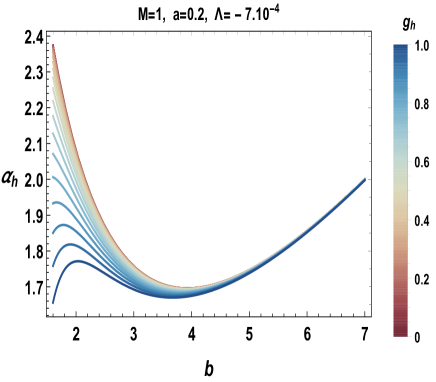
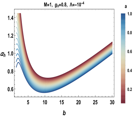
Figure 1: Deflection angle variation of Hayward black holes with cosmological constant in terms of the impact parameter.

For small values of the impact parameter, it has been remarked that the deflection angle of light rays is a decreasing function with a remarkable $g_{h}$ effect. Indeed, it decreases with such a parameter. For large values of the impact parameter, however, the deflection angle of light rays becomes increasing functions with coinciding one dimensional real curves for generic values of $g_{h}$. Moreover, we observe similar effect contributions appearing in the ordinary black hole solutions where the deflection angle decreases by increasing the rotation parameter. The obtained results confirm that the space-time of the ordinary solutions could be affected by $g_{h}$.

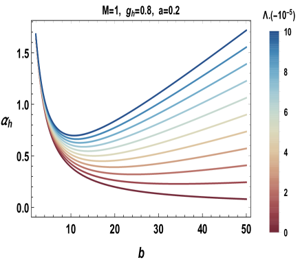
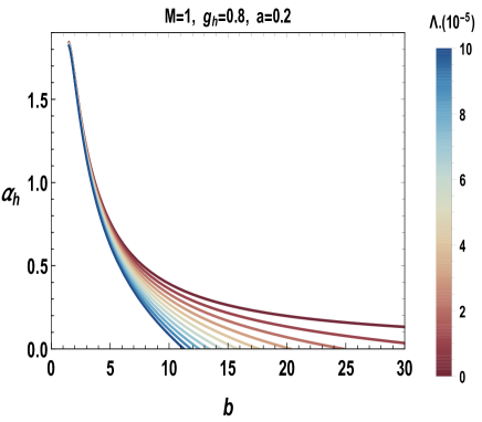
Figure 2: Deflection angle variations of Hayward black holes in terms of the impact parameter $b$ for negative and positive values of $\Lambda$.

To analyze the cosmological constant effect, the deflection angle in terms of $b$ for various values of $\Lambda$ will be inspected. The geometry pushes one to deal with different backgrounds by considering negative and positive values of $\Lambda$. These behaviors are presented in Fig.(2). The analysis depends on two regions associated with the impact parameter values. To do so, we consider first small values of the impact parameter. For small negative values of the cosmological constant, we have remarked a critical behavior where the deflection angle takes a minimal value which augments by decreasing the cosmological constant $\Lambda$. For positive values, however, the deflection angle remains a decreasing function of $b$. For large values of the impact parameter, we have observed that the cosmological constant effect is relevant. Among others, we remark a linear effect of the deflection angle of light rays.

For the Bardeen solutions, the behaviors of the light deflection angle are plotted in Fig.(3).

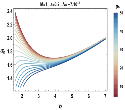
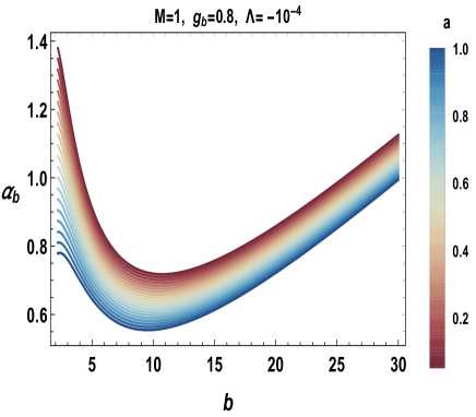
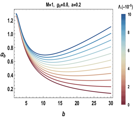
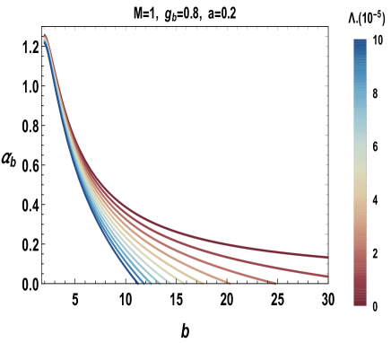
Figure 3: Deflection angle variations of Bardeen black holes with cosmological constant in terms of the impact parameter.

It has been observed similar global behaviors as the previous black hole solutions, where we have identified the same parameter effects. In particular, the finding results match perfectly with the fact that the space-time of the ordinary solutions could be affected by $g_{h}$. However, to unveil certain local distinctions between the regular black hole backgrounds, we present a comparative analysis. In terms of the Kerr solutions with cosmological contributions, indeed, the deflection angle of light rays can be reduced to

$$\alpha_{Kerr}^{\Lambda}\sim\frac{4M}{b}-\frac{4aM}{b^{2}}+\frac{b\Lambda M}{3}-\left(\frac{1}{u_{R}}+\frac{1}{u_{S}}\right)\frac{b\Lambda}{6}+\left(\frac{1}{u_{R}}+\frac{1}{u_{S}}\right)\frac{2a\Lambda}{3}.$$ (5.1)

In Fig.(4), we illustrate the behavior of the deflection angle of the light rays for the regular black hole solutions as a function of the impact parameter, compared with the Kerr solutions.

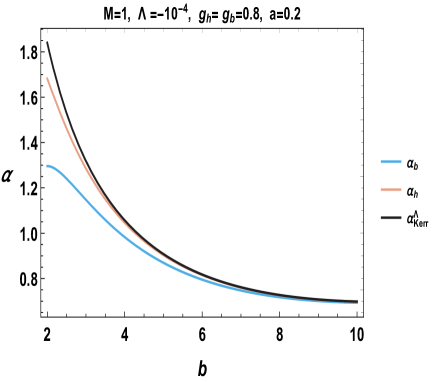
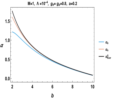
Figure 4: Deflection angle variations of Bardeen, Hayward and Kerr black holes with a cosmological constant .

It has been revealed that small ranges of $b$ are relevant in such an analysis for positive and negative cosmological constant values. However, large values do not bring notable distinctions due to coinciding real curves. It has been remarked that the negative values of the cosmological constant increase the light deflection angle compared with positive ones. Indeed, all solutions involve the same deflection angle of light rays. In this way, the discussion concerns the first range. Indeed, it has been remarked that the deflection angle of light rays by the Bardeen black holes is smaller than the one obtained for Hayward solutions. Moreover, the light defection angle of both solutions is smaller than the Kerr solution one. This result agrees with the previous one showing that the non-linear electrodynamic charges affect the space-time geometry. Such parameters decrease the deflection angle of light rays. We could anticipate that such an angle for both solutions goes to the one of the the ordinary rotating black holes with the cosmological constant. In particular, it has been cheeked that we can recover other findings by sending the cosmological constant to zero[34, 43, 33].

6 Conclusion

In this work, we have studied the weak gravitational lensing for the rotating regular black holes with cosmological contributions. Considering the photon motion in the equatorial plane framework, we have obtained the optical metric needed to provide the associated orbit equations. Using the Gauss-Bonnet theorem results, we have first elaborated the light deflection angle relation of the Hayward solutions by using convenable approximations. The obtained expression has recovered the previous findings. Similar computations have been applied to rotating regular Bardeen black hole solutions. The cosmological relevant relations have been established to derive the deflection angle of light rays. As the first regular model, we have generalized certain previous works. In particular, it has been remarked that the non trivial electrodynamics charges affect the space-time geometry. The obtained results have confirmed the previous works.

Moreover, some other works have been recovered by removing such geometrical contributions. To examine the deflection angle of light rays by such regular black holes with a cosmological constant, we have provided a graphical analysis by varying the involved relevant parameters. Fixing the mass parameter, certain regions of the associated moduli space have been used by considering negative and positive values of the cosmological constant. We have obtained extra corrections terms being considered as extended contributions. Vanishing these terms, we have recovered certain optical behaviors. Finally, we have given a comparative observation concerning regular black hole solutions with respect to the Kerr solutions. It has been shown that large values of $b$ do not involve significant distinctions. In the small ranges of $b$, however, the deflection angles of the Bardeen and the Hayward black holes are smaller than the one of the Kerr solutions with a cosmological constant. This finding matches perfectly with the previous results indicating that the non-linear electrodynamic charges affect the space-time geometry by decreasing the deflection angle of light of rays.

This work comes up with certain open questions. One of them may concern other methods being used to compute the deflection angle of light rays. It would be of interest to investigate such an optical data by applying the elliptic formalism exploited in many places. We hope comeback to such an issue in future works.

References

• [1] B. P. Abbott and et al, Observation of Gravitational Waves from a Binary Black Hole Merger, Phys. Rev. Lett. 116 (2016) 061102, arXiv:1602.03837.
• [2] K. Akiyama and al., First M87 Event Horizon Telescope Results. IV. Imaging the Central Supermassive Black Hole, Astrophys. J. L4 (1) (2019) 875, arXiv:1906.11241.
• [3] K. Akiyama and al., First M87 Event Horizon Telescope Results. V. Imaging the Central Supermassive Black Hole, Astrophys. J. L5 (1) (2019) 875.
• [4] K. Akiyama and al., First M87 Event Horizon Telescope Results. VI. Imaging the Central Supermassive Black Hole, Astrophys. J. L6 (1) (2019) 875.
• [5] A. Belhaj, H. Belmahi, M. Benali, A. Segui, Thermodynamics of AdS black holes from deflection angle formalism, Phys. Lett. B 817 (2021) 136313.
• [6] M. Zhang, M. Guo, Can shadows reflect phase structures of black holes?, Eur. Phys. J. C 80 (2020) 790, arXiv:1909.07033.
• [7] D. Kubizňák, R. B. Mann, Mae Teo, Black hole chemistry: thermodynamics with Lambda, Class. Quantum Grav. 34 (2017) 063001, arXiv:1608.06147.
• [8] A. Belhaj, M. Chabab, H. El Moumni, K. Masmar, M. B. Sedra, A. Segui, On heat properties of AdS black holes in higher dimensions, JHEP. 05 (2015) 149, arXiv:1503.07308.
• [9] A. Belhaj, M. Chabab, H. El Moumni, L. Medari, M. B. Sedra, The thermodynamical behaviors of Kerr–Newman AdS black holes, CPL. 30 (2013) 090402, arXiv:1307.7421.
• [10] A. Belhaj, M. Chabab, H. El Moumni, M. B. Sedra, On thermodynamics of AdS black holes in arbitrary dimensions, Chin. Phys. Lett. 29 (2012) 100401, arXiv:1210.4617.
• [11] S. W. Hawking, D. N. Page, Thermodynamics of black holes in anti-de Sitter space, Commun. Math. Phys. 87 (4) (1983) 577.
• [12] A. Rajagopal, D. Kubiznak, R. B. Mann, Van der Waals black hole, Phys. Lett. B 737 (2014) 277, arXiv:1408.1105.
• [13] Y. Liu, D. C. Zou, B. Wang, Signature of the Van der Waals like small-large charged AdS black hole phase transition in quasinormal modes, JHEP. 09 (2014) 179, arXiv:1405.2644.
• [14] A. Övgün, I. Sakalli, J. Saavedra, Shadow cast and Deflection angle of Kerr-Newman-Kasuya spacetime, JCAP. 10 (2018) 041, arXiv:1807.00388.
• [15] A. Belhaj, H. Belmahi, M. Benali, W. El Hadri, H. El Moumni, E. Torrente-Lujan, Shadows of 5D Black Holes from string theory, Phys. Lett. B 812 (2021) 136025, arXiv:2008.13478.
• [16] A. Belhaj, M. Benali, A. El Balali, W. El Hadri, H. El Moumni, E. Torrente-Lujan, Black hole shadows in M-theory scenarios, Int. J. Mod. Phys. D 30 (2021) 2150026, arXiv:2008.09908.
• [17] J. R. Farah, D. W. Pesce, M. D. Johnson, L. L. Blackburn, On the approximation of the black hole shadow with a simple polar curve, Astrophys. J. 900 (2020) 77, arXiv:2007.06732.
• [18] R. Konoplya, Shadow of a black hole surrounded by dark matter, Phys. Lett. B 795 (2019) 1, arXiv:1905.00064.
• [19] S. V. M. C. B. Xavier, P. V. P. Cunha, L. C. B. Crispino, C. A. R. Herdeiro, Shadows of charged rotating black holes: Kerr–Newman versus Kerr–Sen, Int. J. Mod. Phys. D 29 (2020) 2041005, arXiv:2003.14349.
• [20] S. U. Khan, J. Ren, Shadow cast by a rotating charged black hole in quintessential dark energy, Phys. Dark Univ. 30 (2020) 100644, arXiv:2006.11289.
• [21] X. Hou, Z. Xu, J. Wang, Rotating black hole shadow in perfect fluid dark matter, JCAP 12 (2018) 040.
• [22] S. W. Wei, Y. C. Zou, Y. X. Liu, R. B. Mann, Curvature radius and Kerr black hole shadow, JCAP 08 (2019) 030, arXiv:1904.07710.
• [23] W. Javed, J. Abbas, A. Övgün, Effect of the quintessential dark energy on weak deflection angle by Kerr Newmann Black hole, Annals of Physics 418 (2020) 168183, arXiv:2007.16027.
• [24] A. Belhaj, M. Benali, A. El Balali, H. El Moumni, S-E. Ennadifi, Deflection angle and shadow behaviors of quintessential black holes in arbitrary dimensions, Class. Quantum Grav. 37 (2020) 215004, arXiv:2006.01078.
• [25] W. Javed, J. Abbas, A. Övgün, Deflection angle of photon from magnetized black hole and effect of nonlinear electrodynamics, Eur. Phys. J. C, 79 (2019) 694, arXiv:1908.09632.
• [26] W. Javed, A. Hamza, A. Övgün, Effect of nonlinear electrodynamics on the weak field deflection angle by a black hole, Phys. Rev. D 101 (2020) no.10, 103521, arXiv:2005.09464.
• [27] M. Okyay, A. Övgün, Nonlinear electrodynamics effects on the black hole shadow, deflection angle, quasinormal modes and greybody factors, JCAP 01 (2022) no.01, 009, arXiv:2108.07766.
• [28] J.R. Villanueva, J. Saavedra, M. Olivares, N. Cruz, Photons motion in charged Anti-de Sitter black holes, Astrophys. Space Sci. 344 (2) (2013) 437.
• [29] G. W. Gibbons, M. Vyska, The application of Weierstrass elliptic functions to Schwarzschild null geodesics, Class. Quantum Grav. 29 (2012) 065016, arXiv:1110.6508.
• [30] T. Ono, A. Ishihara, H. Asada, Gravitomagnetic bending angle of light with finite-distance corrections in stationary axisymmetric spacetimes, Phys. Rev. D 96 (2017) 104037, arXiv:1704.05615.
• [31] A. Ishihara, Y. Suzuki, T. Ono, T. Kitamura, H. Asada, Gravitational bending angle of light for finite distance and the Gauss-Bonnet theorem, Phys. Rev. D 94 (2016) 084015, arXiv:1604.08308.
• [32] A. Övgün, Weak field deflection angle by regular black holes with cosmic strings using the Gauss-Bonnet theorem, Phys. Rev. D 99 (2019) no.10, 104075, arXiv:1902.04411.
• [33] G. W. Gibbons, M. C. Werner, Applications of the Gauuss–Bonnet theorem to gravitational lensing, Class. Quantum Grav. 25 (23) (2008) 235009, arXiv:0807.0854.
• [34] K. Jusufi, A. Övgün, J. Saavedra, Y. Vásquez, P. A. González, Deflection of light by rotating regular black holes using the Gauss-Bonnet theorem, Phys. Rev. D 97 (2018) 124024, arXiv:1804.00643.
• [35] R. Penrose, Gravitational collapse and space-time singularities, Phys. Rev. Lett. 14 (1965)57-59.
• [36] S. W. Hawking and R. Penrose, The Singularities of gravitational collapse and cosmology, Proc. Roy. Soc. Lond. A 314 (1970) 529-548.
• [37] V. P. Frolov, M. A. Markov and V. F. Mukhanov, Through a black hole into a new universe?, Phys. Lett. B 216 (1989) 272-276
• [38] V. P. Frolov, Notes on nonsingular models of black holes, Phys. Rev. D 94 (2016) 104056, arXiv:1609.01758.
• [39] E. Ayon-Beato and A. Garcia, Regular black hole in general relativity coupled to nonlinear electrodynamics, Phys. Rev. Lett. 80 (1998) 5056-5059, arXiv:gr-qc/9911046.
• [40] L. Modesto, Black hole interior from loop quantum gravity, Adv. High Energy Phys. 2008 (2008) 459290 [arXiv:gr-qc/0611043 [gr-qc]].
• [41] A. G. Tzikas, Bardeen black hole chemistry, Phys. Lett. B 788 (2019) 219, arXiv:1811.01104.
• [42] M. Molina, J. R. Villanueva, On the thermodynamics of the Hayward black hole, Class. Quant. Grav. 38 (2021) 105002, arXiv:2101.07917.
• [43] S. Haroon, M. Jamil, K. Jusufi, K. Lin, R. B. Mann, Shadow and Deflection Angle of Rotating Black Holes in Perfect Fluid Dark Matter with a Cosmological Constant, Phys. Rev. D 99 (2019) 044015, arXiv:1810.04103.