Red Dragon: A Redshift-Evolving Gaussian Mixture Model for Galaxies

Abstract

Precision-era optical cluster cosmology calls for a precise definition of the red sequence (RS), consistent across redshift. To this end, we present the Red Dragon algorithm: an error-corrected multivariate Gaussian mixture model (GMM). Simultaneous use of multiple colors and smooth evolution of GMM parameters result in a continuous RS and blue cloud (BC) characterization across redshift, avoiding the discontinuities of red fraction inherent in swapping RS selection colors. Based on a mid-redshift spectroscopic sample of SDSS galaxies, a RS defined by Red Dragon selects quenched galaxies (low specific star formation rate) with a balanced accuracy of over $90\%$. This approach to galaxy population assignment gives more natural separations between RS and BC galaxies than hard cuts in color–magnitude or color–color spaces. The Red Dragon algorithm is publicly available at bitbucket.org/wkblack/red-dragon-gamma.

1 Introduction

Galaxies cluster not only in physical space, but in color space as well (Strateva et al., 2001; Bell et al., 2004). The advent of CCD technology revealed a strong dichotomy in galaxy colors: a tightly-packed red sequence (RS; predominantly quiescent, passively evolving ellipticals) and a broader blue cloud (BC; predominantly active, star-forming spiral galaxies) (Bower et al., 1992; Schawinski et al., 2014). Galaxies that fall between the RS and BC populate the ‘green valley’ (GV).

Astrophysically, the RS serves as an imperfect proxy for selecting galaxies with low specific star formation rate (sSFR). Star formation decays naturally with age: stellar populations older than roughly $1~{}{\rm Gyr}$ become almost uniformly red, implying that the reddest galaxies have essentially no star formation (Conroy & Gunn, 2010). Due to the Gaussian random nature of $\Lambda$CDM initial conditions, the density of peaks on different scales are coupled, such that the earliest forming galaxies reside in regions destined to host clusters of galaxies (Springel et al., 2005). As a result, clusters naturally contain an older galaxy population than the field. Other dynamical processes that can shut down star formation are also enhanced in proto-cluster environments. Major mergers between galaxies cause rapid morphological and chromatic shifts from blue spirals towards red ellipticals. Effects such as ram-pressure stripping and AGN feedback blow away gas from high density regions, rapidly diminishing star formation—or quenching—the galaxy (Schawinski et al., 2014). Galaxy clusters are natural hotbeds for merging, ram-pressure stripping, and AGN feedback as well, so they serve as ideal nodes at which to find quenched galaxies.

The distribution of sSFR is skew-lognormal, with a peak of blue active star-forming galaxies at ${\rm sSFR}\sim 10^{-10}~{}{\rm yr}^{-1}$ at low redshift (the galactic main sequence) and a tail towards lower sSFR (Wetzel et al., 2012; Eales et al., 2018). This form suggests that the sSFR frequency distribution could be modeled as a dual Gaussian mixture. Further strengthening this duality, the scatter in photometric color decreases drastically as sSFR decreases, such that galaxies with ${\rm sSFR}\lesssim 10^{-11.3}~{}{\rm yr}^{-1}$ share approximately the same color (Eales et al., 2017), thus creating an exceptionally narrow distribution of colors for quiescent galaxies. These factors combined then produce a dual Gaussian in photometric color (see e.g. Baldry et al., 2004; Hao et al., 2009): a narrow component for the low-sSFR RS and a wider component for the high-sSFR BC.

Since the red sequence is particularly strong in clusters, it serves as a strong key for galaxy cluster selection. Identification of clusters by their RS was first proposed by Gladders & Yee (2000). Since galaxies redden with age, ignoring galaxies bluer than a given cluster’s RS removes essentially all galaxies at lower redshifts, efficiently reducing foreground contributions. The maxBCG algorithm (Koester et al., 2007) further improved cluster selection, using a hard $\pm 2\,\sigma_{\rm RS}$ cut in photometric color to select clusters. The algorithm defines richness, $N_{200}$, as the count of red galaxies within an estimated virial radius, $R_{200}$. This count of virialized galaxies within the cluster serves as a halo mass proxy (Rozo et al., 2009a). Rozo et al. (2009b) developed an improved richness estimate $\lambda$: the sum of RS membership probabilities for a given cluster, which included a more nuanced cutoff radius and a Gaussian color filter.

More recent algorithms and surveys have extended the RS’s use for cluster cosmology. To further improve the red/blue galaxy distinction, Hao et al. (2009) developed a single-color error-corrected Gaussian Mixture Model (ECGMM) in color-magnitude space. As compared to a typical GMM, their ECGMM accounted for photometric errors contributing to the scatter. Again, they selected RS galaxies within a hard $\pm 2\sigma_{\rm RS}$ cut. Around this time, the first results from the SpARCS survey (The Spitzer Adaptation of the Red-sequence Cluster Survey; Wilson et al., 2009; Muzzin et al., 2009) produced hundreds of $z>1$ cluster candidates using a selection method similar to that of Gladders & Yee (2000). Later, Rykoff et al. (2014) designed the redMaPPer algorithm, which selects RS galaxies in a multi-color + magnitude space, giving a redshift-continuous, multi-color update to richness. Building on similar methodology, Rozo et al. (2016) introduced the redMaGiC algorithm to select luminous red galaxies, estimating galactic redshifts with high accuracy. These methods serve as a basis for DES cluster finding in cosmological analyses (Rykoff et al., 2016; Abbott et al., 2020), with the richness indicator $\lambda$ serving as a mass proxy.

We present Red Dragon: a multivariate Gaussian mixture model to select the RS along with other galactic populations. Red Dragon gives a consistent RS definition and continuous red fraction across redshift, characterizing well the underlying photometric distribution of galaxies.

Red Dragon follows the historical trend of moving from quantized (e.g. binary) classifications towards continuous, probabilistic definitions. Where once galaxies were purely classified as ellipticals or spirals, continuous morphological parameters now allow for more precise morphological characterization of galaxies (Conselice, 2014). Similarly, the RS has historically been selected as a hard cut in color–magnitude (e.g. Hao et al., 2009) or color–color space (e.g. Whitaker et al., 2012), but these cuts lack the nuanced information available from the full multi-color space of 4+ band surveys. Red Dragon now offers a probabilistic and smooth RS definition across redshift.

We begin in section 2 by introducing the datasets used in this analysis, along with an extended discussion of motivations for our method. Section 3 then details the truth labels used to quantify goodness of RS fit and expounds technical features of the algorithm, such as the optimal number of Gaussian components to use. Section 4 presents several results of this method. Finally, section 5 summarizes the method and discusses future applications.

2 Data & Motivations

In this section, we introduce the three datasets used in this work (§2.1) then explain several of our chief motivations in developing this algorithm: chiefly the redshift drift of the 4000 Å break (§2.2) and the information to be gained from multi-color analysis (§2.3).

2.1 Datasets

Table 1: The various datasets used in this analysis. The baryon pasting algorithm ADDGALS created Buzzard’s synthetic galaxy catalog, assigning SDSS-like galaxies to an underlying N-body simulation.

Dataset	Type	Redshift	sSFR	$N_{\rm gal}$
SDSS/low-$z$	Observation	$0.1\pm 0.005$	Yes	44 452
SDSS/mid-$z$	Observation	$(.3,.5)$	Yes	90 609
TNG300-1	Hydro sim	$0.1$	Yes	62 230
Buzzard	Synthetic	$[0.05,0.84]$	No	91 004 552

We analyze galaxies from the three datasets listed in table 1: local observed galaxies from SDSS (Szalay et al., 2002), galaxies at low redshift produced by the hydrodynamic simulation IllustrisTNG (Nelson et al., 2018, Model C, observed frame), and a wide redshift sample from the Buzzard Flock synthetic galaxy catalog (DeRose et al., 2019, 2021). All galaxy samples are luminosity limited such that $L_{i}(z)>0.2\,L_{*,i}(z)$ using the $i$-band characteristic luminosity as a function of redshift, $L_{*,i}(z)$ as defined in Rykoff et al. (2014). These samples offer complementary tests of Red Dragon’s ability to identify the quiescent galaxies of the RS.

SDSS galaxies were selected from a spectroscopic sample. For the low-redshift $z=0.1\pm.005$ sample, redshift errors were typically $\lesssim 10^{-4}$. We limit summed photometric error to be below $0.3$ to exclude galaxies with poor photometry. Specific star formation rates were calculated using methods from Conroy et al. (2009) and are employed as a truth label to test against Red Dragon’s selection of quenched galaxies. The other SDSS galaxy sample, spanning redshifts $0.3$ to $0.5$, tests Red Dragon’s ability to smoothly select red galaxies as the 4000 Å break crosses filters. This sample has typical redshift error $\lesssim 10^{-3}$, and our required redshift error of less than 0.05 excludes fewer than one in $10^{4}$ galaxies.

We also use the Illustris TNG300-1 cosmological hydrodynamic simulation at redshift $z=0.1$ (with synthesized SDSS photometry). These galaxies have a truth label for sSFR derived from each galaxy’s star formation history. As noted in section 4.1.1 and as illustrated in appendix A, the distributions of galaxy colors do not match well those of SDSS, making application to this sample more so a test of Red Dragon’s robustness than of its RS selection capacity.

The Buzzard synthetic galaxy catalog is a wide-area galaxy sample that extends the redshift range of our analysis to $z=0.84$. To create the Buzzard galaxy catalog, the ADDGALS algorithm (Busha & Wechsler, 2008; Wechsler et al., 2021) populated lightcone outputs of N-body simulations with galaxies. The empirical method introduces galaxy bias using a local dark matter density measure, and colors are applied using templates tuned to SDSS and other observed galaxy samples. The method reproduces well the magntitude counts and two-point clustering of galaxies at $z<1$, but massive clusters are somewhat underpopulated as compared to observations (DeRose et al., 2021; Wechsler et al., 2021).

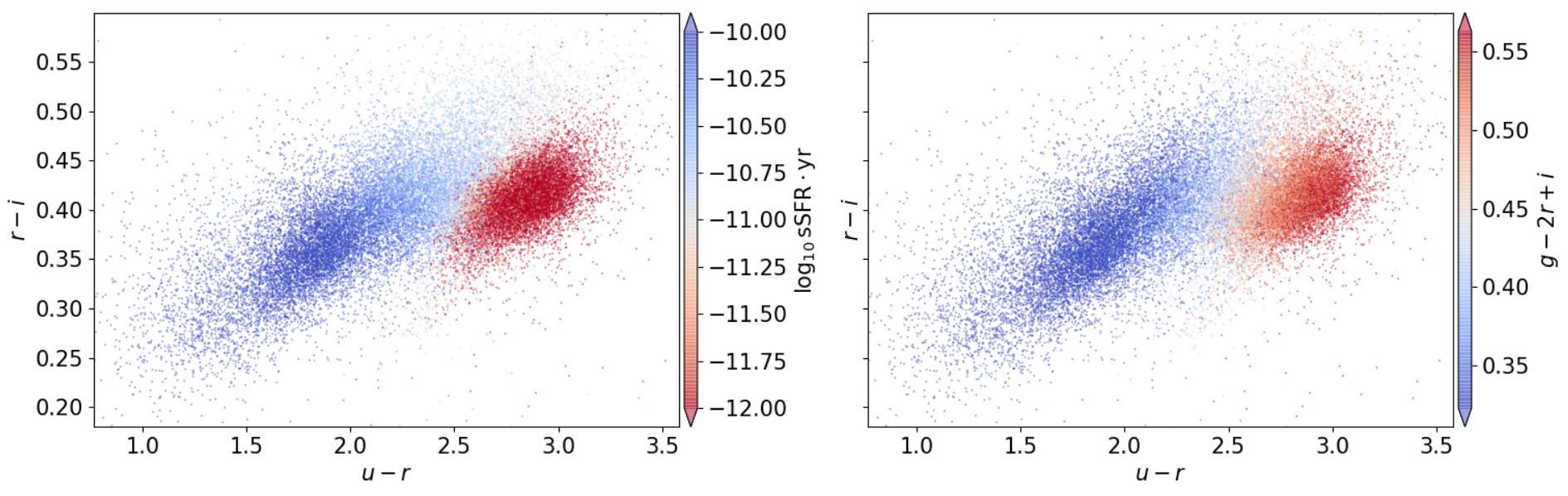
Figure 1: SDSS low-redshift galaxy sample ($z=0.1\pm 0.005$) plotted in CC space. The color $u-r$ gives a relatively clean measurement of the strength of the 4000 Å break, measuring current SFR. The color $r-i$ measures the post-break slope, an indicator of dust content (somewhat degenerate with age and metallicity). Left: colored by log specific star formation rate, with values below roughly -11 corresponding to the quenched population. Right: colored by $g-2r+i$, a pseudo finite difference second derivative near the 4kÅ break, corresponding roughly with metallicity.

2.2 Redshift drift of 4000 Å break

Our main motivation in creating the Red Dragon algorithm originated in the redshift drift of “the 4000 Å break”: a sharp drop in spectral intensity at short wavelengths and the primary effect of quenching on a galaxy’s spectrum. This break has two main sources. Though only certain wavelengths larger than 3645 Å can be absorbed by excited ($n=2$) Hydrogen, any wavelength shorter than that will fully ionize an electron. This asymptote of the Balmer series at 3645 Å results in a sharp drop of intensity towards shorter wavelengths (Mihalas, 1967). Meanwhile, stellar production of metals results in a blanket of line absorption, reddening the spectrum around 4000 Å (Worthey, 1994). These two effects conspire to cause a strong suppression of emission at wavelengths shorter than $3800\pm 200$ Å.

Table 2: Approximate redshift ranges over which each band will measure 4kÅ rest wavelengths, given for both SDSS (Doi et al., 2010) and DES (Abbott et al., 2018) photometries.

band	$z_{\rm break,SDSS}$	$z_{\rm break,DES}$
g	$[0.0,0.36)$	$[0.0,0.38)$
r	$[0.36,0.71)$	$[0.38,0.78)$
i	$[0.71,1.06)$	$[0.78,1.13)$
z	$[1.06,1.37)$	$[1.13,1.50)$
Y	N/A	$[1.38,1.55)$

Table 2 shows approximate redshifts at which a rest frame wavelength of 4000 Å is observed in each observational band for both SDSS and DES. The difference in magnitude of the bands surrounding the band in which the break resides gives the cleanest measure of D4000 (the ratio of intensity on either side of the break), which gives an excellent estimate of sSFR. The optimal photometric color for RS selection thus changes with redshift.

If a RS selector uses only one color at a time, with discrete jumps in photometric color at certain transition redshifts, these hard transitions can result in an $\mathcal{O}(10\%)$ shift in red fraction, $f_{R}(z)$ (up to $\sim 16\%$; see e.g. Nishizawa et al., 2018). This jolt in red fraction would echo in single-color richness estimates based on a count of bright red galaxies in a cluster. Two identical clusters on either side of a redshift transition could then have significantly different $\lambda_{\rm col}$ values, introducing non-trivial systematic errors in halo mass–richness scaling relations.

Evolving a multi-color Gaussian mixture across redshift smoothly defines the RS, obviating the discontinuities caused by color swapping. Taking all colors into account simultaneously allows for a continuous and consistent RS out to high redshifts.

2.3 Beyond the 4000 Å break

Though a galaxy’s quenched status primarily manifests though the strength of D4000, other astrophysical factors such as age, dust, or metallicity separate RS from BC photometrically. (For a summary of main effects of galaxy properties on optical spectra, see Figure 13.) Though D4000 can be estimated using a single photometric color, multi-color analysis serves to better distinguish the RS from the BC.

Figure 1 illustrates this for the low-$z$ SDSS galaxy sample. While the horizontal axis $(u-r)$ correlates highly with D4000, the vertical axis $(r-i)$ gives a degenerate measure of dust content and other properties. The left panel colors points by specific star-formation rate (where $\log_{10}{\rm sSFR}\sim-11$ separates quenched from star-forming galaxies) while the right panel colors points by $(g-2r+i)$. The latter visibly correlates with the former.

This composite feature of $(g-2r+i)$ acts as a pseudo second derivative, approximating here the spectrum curvature near the 4000 Å break. While ordinary single-color (a vertical line on this plot) or CC selection (an angled line on this plot) would be ignorant of such information, the curvature information clearly correlates with sSFR and would aid in selecting the quenched population. Even a perfectly positioned hard line cut would be inherently limited in selecting quenched galaxies (see Figure 4).

A multi-color Gaussian mixture simply includes such curvature terms using the primary color space (i.e. differences between neighboring bands; see equation 5). Here we have $(u-r)=(u-g)+(g-r)$ and $(g-2r+i)=(g-r)-(r-i)$, showing up as $\pm 45^{\circ}$ directions in the multi-dimensional primary color space. Furthermore, the populations overlap in both CM and CC spaces, limiting the power of hard cut selection. In contrast, Gaussian mixtures are designed to model such overlapping populations, making them a natural tool to consider in selecting the RS and BC.

In order to combat $f_{R}(z)$ discontinuities, move beyond hard cuts in photometry, and better select the photometry-space population of RS galaxies, we present the Red Dragon algorithm.

3 Methods

Red Dragon is a novel method for calculating red sequence membership probabilities $P_{\rm RS}$. In its most general construction, a Red Dragon RS selector uses a Gaussian mixture in multi-color space to select populations of galaxies (RS, BC, and optionally additional components). In §3.1, we outline the algorithm, including the sequence of operations and the relevant likelihood function. Considerations when applying the algorithm are presented in §3.2, discussing choices such as the optimal number of colors or model components.

3.1 Algorithm Construction

Here we give an overview of the algorithm (§3.1.1), introduce the core likelihood function for Red Dragon (§3.1.2), and detail interpolation of GMM parameters across redshift (§3.1.3).

3.1.1 Overview of algorithm

Figure 2: Work flow for RD algorithm. The process has two main portions: (1–4) moving from input data to creating GMM parameterizations $\{\vec{\theta}_{\alpha}\}_{i}$ at each redshift slice $i$ and (4–7) interlinking components across redshift from the disarranged collection $\{\vec{\theta}_{\alpha}\}$ to parameterize redshift-continuous GMM components, $\vec{\theta}_{\alpha}(z)$, and thereby membership probabilities $P_{{\rm mem},\alpha}(z,\vec{m},\vec{\sigma}_{m})$. The grey arrow (8) indicates that after a dragon is created, it may be used to initialize components in fitting the GMM. This is especially useful for outlier redshift bins which didn’t fit like their neighbors. By default, the algorithm does a single pass (1–7) fitting sparsely with the sklearn GMM, then uses that fit to inform initial conditions for the pyGMMis GMM, which gives the second pass (4–7) for a final fitting.

Broadly speaking, there are two stages to the Red Dragon algorithm, as illustrated in Figure 2. In the first stage, it segments the data into discrete redshift shells and finds GMM parameterizations for each slice. In the second stage, it matches components across redshift bins and interpolates parameters. This results in continuous and consistent definition of the RS and BC (and optionally further components).

First stage: redshift-discrete fits.

Red Dragon reads in photometry and redshift information as supplied by the user (see the values in Figure 2, box 1). Input redshift estimates $z$ and errors $\delta_{z}$ allow for binned analysis of redshift evolution. From input magnitudes $\vec{m}$ and magnitude errors $\vec{\delta}_{m}$, Red Dragon calculates colors $\vec{c}$ and the corresponding noise covariance matrix $\Delta$ (see equation 4). This set of input variables are then sent to a GMM to find fit parameters $\vec{\theta}_{\alpha}$ in each redshift bin. See section 3.1.2 for details on the likelihood model and fitting process.

At this point, the algorithm has saved as output data $\{\vec{\theta}_{\alpha}\}_{i}$, i.e. at each redshift bin $i$ and for each component $\alpha$, it saves Gaussian mixture parameters $\vec{\theta}$ (see table 3). These components are unordered at this point, so the $\alpha=0$ component in redshift bin $i=1$ may not correspond to the $\alpha=0$ component in redshift bin $i=2$. This set of Gaussian parameterizations must be linked across redshift continuously to avoid spurious rapid changes of classification over small redshift ranges.

Second stage: redshift-continuous fits.

Using the calculated set of Gaussian mixtures, $\{\vec{\theta}_{\alpha}\}_{i}$, the algorithm now matches similar Gaussian components across redshift bins. While distinguishing continuous components across redshift is relatively simple for two-component models ($K=2$), matching for even three components ($K=3$) can be challenging. (Does the wide, redder portion of the BC connect to the narrower but similar in color component in the adjacent redshift bin, or does it connect to the component with similar scatter despite its significantly bluer color?) Despite these challenges, the matching process can be largely automated, as discussed in appendix G.

After successful matching across redshift bins, the now linked set of parameters $\{\vec{\theta}_{\alpha^{\prime}}\}_{i}$ can then be interpolated across redshift, giving the continuous parameterizations $\vec{\theta}_{\alpha}(z)$. These continuously evolving Gaussian components can then yield component membership probabilities for a galaxy at a given redshift with given photometry for each component $\alpha$: $P_{\rm mem,\alpha}(z,\vec{m},\vec{\delta}_{m})$. This interpolated parameterization now presents the user with a trained dragon, smoothly characterizing each of the populations across redshift.

3.1.2 Likelihood model

$\theta_{\alpha}$	model parameters	$x_{j}$	galaxy data
$w_{\alpha}$	weight (where $\sum_{\alpha}w_{\alpha}=1$)	$\vec{c}_{j}$	color
$\vec{\mu}_{\alpha}$	mean color	$\vec{\delta}_{j}$	errors on galaxy colors
$\Sigma_{\alpha}$	intrinsic covariance	$\Delta_{j}$	noise covariance

Table 3: Summary of variables in likelihood model (see equations (7) and (6)). Left column shows GMM model parameters $\theta_{\alpha}$ characterizing component $\alpha$ of $K$; right column shows input data for galaxy $j$ of $N_{\rm gal}$. Galaxy colors, with their respective errors and noise covariance, are calculated from input magnitudes $\vec{m}\pm\vec{\delta}_{m}$ within redshift bins (determined by galaxy $z\pm\delta_{z}$).

Red Dragon employs a multi-dimensional Gaussian mixture model which accounts for photometric errors; parameters of the Gaussian mixture evolve with redshift to give continuous characterizations of each GMM component.

A Gaussian mixture of $K$ components in a single color $c$ has a set of parameters $\theta$ that constitute the model. For each component $\alpha$, this parameter set includes the component weight $w_{\alpha}$, mean color $\mu_{\alpha}$, and the intrinsic population scatter $\sigma_{\alpha}$ (see table 3 for a summary of parameters used). The weights are normalized such that $\sum_{\alpha}w_{\alpha}=1$. For a set of $N_{\rm gal}$ galaxies with input colors $\{c_{j}\}$, and color errors $\{\delta_{i}\}$, the model parameters maximize the likelihood

$$\mathcal{L}(\theta\big{|}x)=\prod_{j=1}^{N_{\rm gal}}\left\{\sum_{\alpha=1}^{K}\frac{w_{\alpha}}{\sqrt{2\pi({\sigma_{\alpha}}^{2}+{\delta_{j}}^{2})}}\exp\left[-\frac{1}{2}\frac{(c_{j}-\mu_{\alpha})^{2}}{{\sigma_{\alpha}}^{2}+{\delta_{j}}^{2}}\right]\right\}.$$ (1)

This type of error-corrected Gaussian mixture model (ECGMM) was introduced by Hao et al. (2009) with SDSS $g-r$ as the color classifier.

Expanding this model into an $N$-dimensional color space requires that we employ for each component $\alpha$ an intrinsic color covariance matrix $\Sigma_{\alpha}$. The errors then must be handled as a noise covariance matrix $\Delta_{i}$ for each galaxy.

Consider the DES four-band optical $griz$ photometry used in Buzzard, with input magnitudes $\vec{m}=[m_{g},\,m_{r},\,m_{i},\,m_{z}]$. We define a vector of primary colors based on neighboring photometric bands:

$$\vec{c}=[g-r,\,r-i,\,i-z].$$ (2)

Colors are derived from magnitudes by the matrix operation $\vec{c}=A\,\vec{m}$, where the transform matrix is

$$A=\begin{bmatrix}1&-1&0&0\\ 0&1&-1&0\\ 0&0&1&-1\end{bmatrix}.$$ (3)

We assume that the photometric errors of each galaxy are determined independently in each band, and so take them to be uncorrelated. The magnitude error covariance matrix $M_{j}$ for each galaxy is then diagonal. Transformed to the space of primary colors (equation (2)), the noise covariance of galaxy $j$ is then

$$\Delta_{j}=A\,M_{j}\,A^{\top}=\begin{bmatrix}{\delta_{g}}^{2}+{\delta_{r}}^{2}&-{\delta_{r}}^{2}&0\\ -{\delta_{r}}^{2}&{\delta_{r}}^{2}+{\delta_{i}}^{2}&-{\delta_{i}}^{2}\\ 0&-{\delta_{i}}^{2}&{\delta_{i}}^{2}+{\delta_{z}}^{2}\end{bmatrix}_{j}$$ (4)

where $\delta_{x}$ above refer to the photometric error of band $x$ for galaxy $j$. Note that for this matrix to be non-singular, the selection of colors must be linearly independent (e.g. one cannot use each of $g-r$, $r-i$, and $g-i$ in an error-inclusive model). For symmetry, simplicity, and to avoid singularity, we employ the set of primary colors.

The derivation of $\Delta_{j}$ is similar for SDSS photometry (which includes $u$ band). The primary color vector for $ugriz$ is then

$$\vec{c}=[u-g,\,g-r,\,r-i,\,i-z]$$ (5)

and the corresponding $\Delta_{j}$ matrices come from a straightforward extension of the above matrices.

This likelihood of this error-cognizant $N$-dimensional Gaussian mixture model is then

$$\mathcal{L}(\theta\big{|}x)=\prod_{j=1}^{N_{\rm gal}}\sum_{\alpha=1}^{K}\mathcal{L}_{\alpha}(\theta_{\alpha}\big{|}x_{j})$$ (6)

where the likelihood for each galaxy $j$, component $\alpha$, is

$$\mathcal{L}_{\alpha}(\theta_{\alpha}\big{|}x_{j})= \frac{w_{\alpha}}{\sqrt{(2\pi)^{N}}\left|\Sigma_{\alpha}+\Delta_{j}\right|}$$ (7)

$$\times\exp\left[-\frac{1}{2}(\vec{c}_{j}-\vec{\mu}_{\alpha})^{\mathrm{T}}(\Sigma_{\alpha}+\Delta_{j})^{-1}(\vec{c}_{j}-\vec{\mu}_{\alpha})\right].$$

Here, $x_{j}$ includes all primary colors $\vec{c}_{j}$ as well as the noise covariance matrix $\Delta_{j}$ for each galaxy (see table 3).

At individual redshift slices, we use the error-inclusive Gaussian Mixture package pyGMMis (Melchior & Goulding, 2018) to find best-fit parameters $\theta_{\alpha}$ for each component $\alpha$. Without a reasonable input for a first guess at parameters, pyGMMis sometimes struggles to properly characterize populations. To provide a rough first guess, we first sparsely fit the data using sklearn’s error ignorant GaussianMixture package (Pedregosa et al., 2011). This extremely quick fit gives a rough initial guess to the fit parameters, yielding better results than running pyGMMis blind.

3.1.3 Fit interpolation

Red Dragon interpolates best-fit parameters across redshift bins, continuously defining populations. After fitting weights, the normalization $\sum_{\alpha}w_{\alpha}(z)=1$ is re-enforced. To interpolate the covariance matrix, log variances are interpolated first, followed by interpolating the correlations (enforcing $|\rho|\leq 1$), which together then provide a better fit than purely fitting the covariance matrix all at once (which could result in unphysical negative variances). Fitting is linear by default (with flat endpoint extrapolation), but other methods such as smoothed spline interpolation (SciPy: Virtanen et al., 2020) or kernel-localized linear regression (KLLR: Farahi et al., 2018; Anbajagane et al., 2020) are available to give smoother fits.

These redshift-continuous fits can then predict for individual galaxies its membership likelihood for each component. The probability that galaxy $j$ is a member of GMM component $\alpha$ is

$$P_{\alpha}(x_{j})=\frac{\mathcal{L}_{\alpha}(\theta_{\alpha}\big{|}x_{j})}{\sum_{\beta}\mathcal{L}_{\beta}(\theta_{\beta}\big{|}x_{j})}.$$ (8)

A two-component model would then have red sequence membership probability $P_{\rm RS}=\mathcal{L}_{\rm RS}/(\mathcal{L}_{\rm RS}+\mathcal{L}_{\rm BC})$.

This parameterization results in a redshift-continuous definition of the red sequence over large redshift spans, without the jumps or transitions incurred by single or double-color RS selection. Its more objective definition of the RS better characterizes the nuances of galaxy multi-color space than hard cuts.

3.2 Algorithm Considerations

In this section, we define accuracy in selecting the quenched population for this analysis (§3.2.1), detail the accuracy gains from added bands (§3.2.2), discuss the optimal count of Gaussian components (§3.2.3), and discuss whether Gaussian features must be allowed to run with magnitude to accurately select the quiescent population (§3.2.4).

3.2.1 Balanced Accuracy

To quantify goodness of fit for the RS, we use the binary classification measure of ‘balanced accuracy,’ comparing RS members selected by Red Dragon to the quenched population. We convert Red Dragon red component probability to a binary RS classifier by the condition $P_{\rm RS}>0.5$ and defined quenched galaxies using a threshold in specific star formation rate as a function of redshift

$$\log_{10}\left({\rm sSFR}\cdot{\rm yr}\right)<-11+z$$ (9)

(adapted from Moustakas et al., 2013, for our mass and redshift ranges). A more complicated determination of a truth label for the RS could include measures of stellar mass, dust, metallicity, and age as metrics to aid in separating RS and BC (see section 2.3). For example, one could simply add these into a GM or other machine learning structure along with the colors, giving the structure more information to aid in the separation. While such a model may serve as a more accurate truth label to test against, our benchmark hard cut in sSFR defines a straightforward underlying truth in the photometric distribution of galaxies; its strong correlation with idealized galaxy characterization gives it value in discriminating between RS selectors.

Balanced Accuracy (also BA or bACC) takes the average of sensitivity and specificity, i.e. the true positive rate TPR$\equiv$TP/(TP+FN) and the true negative rate TNR$\equiv$TN/(TN+FP). This compensates for unequal population ratios: the relative weight between RS and BC varies significantly across redshift and magnitude, so bACC equally represents selection accuracy between the two populations.

We caution the reader that achieving 100% accuracy is not only practically impossible (without overfitting), but also not quite ideal. Since the sSFR distributions of RS and BC overlap, a hard cut in sSFR to score selection would mischaracterize a set fraction of galaxies from each. More nuanced selection of the RS and BC (defined from the more complicated definition above) would then have an accuracy at some value below 100%, though still high. Therefore, balanced accuracies from a hard cut in sSFR below 100% should be no cause for worry, and indeed, could indicate the method is working properly.

Balanced accuracy requires a binary classification, so it is somewhat limited in its ability to score goodness of fit for ambiguous cases where e.g. the quenched probability $P_{\rm Q}=49\%$ (the chance, taking error bars into account, that equation 9 is true) but the RS membership probability $P_{\rm RS}=51\%$ (the chance, derived from Gaussian Mixtures, that it belongs to the redder component). The sSFR distribution is lognormal skewed, with the bulk of galaxies falling near the sSFR cut of equation (9), so middle probabilities are common, with $\sim 40\%$ of galaxies lying in $P_{Q}|(25,75)\%$. Quenched probabilities are therefore somewhat sensitive to the sSFR cut one uses to define the quenched population; any hard cut in sSFR will necessarily change the resulting bACC. However, the distribution of $P_{\rm RS}$ values is strongly bimodal, with generally $\lesssim 15\%$ of galaxies lying in $P_{\rm RS}|(25,75)\%$ for Buzzard and $\lesssim 1\%$ for SDSS (TNG sSFR values are without errors). Since probabilities generated by Red Dragon tend towards zero and one, the problem of hard cuts in binary classification is somewhat mitigated. A simple binary classification metric aptly characterizes the large majority of galaxies and gives a simple measure for RS selection power.

3.2.2 Accuracy gains from added colors

Typically, single-color RS selection uses a color constructed from the photometric band containing the 4000 Å break and the longer-wavelength band immediately after ($g-r$ at low redshifts); two-color RS selection further includes the primary color with the next longest wavelength band after that ($r-i$ at low redshifts). However, other colors can aid in better distinguishing the RS from the BC.

For SDSS low-$z$, we used all possible colors (including the band-jumping secondary colors, like $g-i$ or $u-z$, in addition to the primary colors; only considering non-singular combinations of colors) to create single, double, and triple color Gaussian mixture models, revealing optimal color combinations along with accuracy gains from adding colors. Comparing these optimized color groupings to our choice of using all primary colors for Red Dragon’s spine, we can gauge to what extent selection accuracy depends on choice of the input color vector $\vec{c}$.

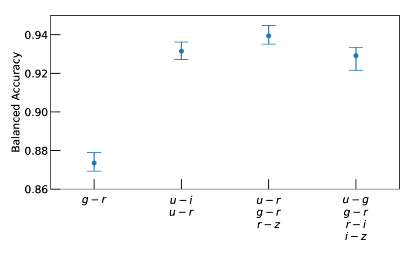
Figure 3: Accuracy of selecting the quenched population in low-$z$ SDSS by Gaussian mixture for various combinations of input colors. Each of the first three $N$-color groupings were optimized in their selection, having the highest median bACC of all possible $N$-color combinations. Error bar plot shows bootstrap $\pm 2\sigma$ quantiles.

Figure 3 shows that for SDSS/low-$z$, single-color selection (using the optimal choices of either $g-r$ or $u-r$), selected the quenched population with $\sim 87\%$ accuracy. Adding a second color significantly improved accuracies (again using optimal band choices from our analysis of all possible colors), raising balanced accuracy immensely ($+5.8\%$). Optimal three-color selection gave a relatively small increase in bACC ($+0.8\%$). The four-color combination of the primary color vector (no optimization of color choices) performed similarly to the best-case three-color combination ($-1.0\%$). The primary color vector thus serves well as a blind baseline for selecting the quenched population.

3.2.3 Optimal Gaussian Component Count

Though historically galaxy classification has been binary, galaxies transitioning from RS to BC are sometimes classified as members of the green valley (GV), adding a third category. From an agnostic view of the color space data, components beyond two can simply be seen as an attempt to better model inherent non-Gaussianities in the populations (see e.g. Carretero et al., 2015). From an astrophysics view, galaxies quenched by different mechanisms belong to populations with distinct characteristics (Peng et al., 2010; Davies et al., 2021; Dacunha et al., 2022). High-mass galaxies (which are primarily mass-quenched) have different trends for mean and scatter of colors than those of low-mass galaxies (which are primarily merger- or environment-quenched) (Baldry et al., 2004), so modeling them with distinct Gaussians could better represent the underlying populations. For any of the above reasons, one may desire to model components beyond two. Though the Red Dragon algorithm permits any number of components $K\geq 2$, different datasets or different luminosity cuts may favor particular component counts.

Appendix C details our analysis of SDSS/low-$z$ for optimal component count. In short, though Figure 1 shows clear bimodality visually, and indeed, using two components gives a fair fit to the photometric color data, using three components fits the distribution of galaxies in photometric color space significantly better. Using more than three components gave no significant improvement in fit. For simplicity of discussion and comparison, we chiefly employ the minimal two-component model in our results section, but an investigation of the effects of increasing component count is detailed in section 4.2.2, using the Buzzard simulation.

3.2.4 Running with magnitude

Gaussian mixture parameters (population weight, mean color, and scatter for RS and BC) are known to depend on magnitude at a fixed redshift. Nearly 100% of bright galaxies are red, while very few of the faintest galaxies are red (Baldry et al., 2004), so component weight runs strongly with magnitude. The mean color of the RS is well-known to run with magnitude (Kodama & Arimoto, 1996; Gladders et al., 1998), with the slope modeled explicitly in the RS fitting of e.g. Hao et al. (2009) and Rykoff et al. (2014). The scatter of the RS and BC also runs non-linearly with magnitude (Baldry et al., 2004; Balogh et al., 2004), though this is less often modeled. Therefore, a magnitude-ignorant fitting of the populations will have all parameters somewhat dependent on the limiting magnitude of the sample. The brighter the sample, the higher the $f_{R}$, the redder the mean RS color, and the smaller the RS scatter. Though parameters do evolve with magnitude, how significantly does magnitude ignorance affect selection of the RS?

Using Buzzard, we quantify differences in RS selection between magnitude-cognizant and magnitude-ignorant models. Appendix D shows results of this analysis. In short, while magnitude running of GMM parameters is statistically significant, their running had a relatively minimal impact on selection.

For thin redshift slices, selection of red sequence galaxies (where $P_{\rm RS}>.5$) was 95% identical between the standard redshift-running and the niche magnitude-running versions of Red Dragon. Since this difference in selection is relatively small, we leave magnitude running out of the current version of Red Dragon in favor for prioritizing smooth redshift evolution. For those who wish to explicitly account for magnitude running or other secondary parameters, several workarounds exist, as detailed in section D.3.

4 Results

Here we show results of running Red Dragon on SDSS, TNG, and Buzzard datasets. Our SDSS+TNG analysis focuses on the accuracy of selecting the quenched population whereas our Buzzard analysis highlights fit parameter evolution with redshift.

4.1 Sloan analysis

We run Red Dragon on Sloan and TNG data using the four primary colors derived from SDSS $ugriz$ photometry, with equation (5) as the primary color vector. Here we present the accuracy with which Red Dragon identifies the quenched galaxy population at low (§4.1.1, including TNG) and intermediate (§4.1.2) redshifts.

Our comparison to typical CM and CC selections follow methods from the literature. ‘Typical’ CM selection follows Hao et al. (2009). After fitting the red sequence population with a Gaussian mixture in color space, we fit a line to the red sequence population (in the CM space of $g-r$ vs $m_{i}$), find its scatter, then select all galaxies within $2\sigma$ of the mean relation. ‘Typical’ CC selection follows Adhikari et al. (2020). After finding population means via Gaussian mixtures, we draw a line between maxima (in the CC space of $g-r$ vs $r-i$), then plot a perpendicular line at the minimum likelihood point between the two components (i.e. where a galaxy is equally likely to belong to either component). These two methods give benchmark comparisons for standard efficiency of selection in CM and CC spaces for comparison to Red Dragon selection.

4.1.1 Selection accuracy of the quenched population

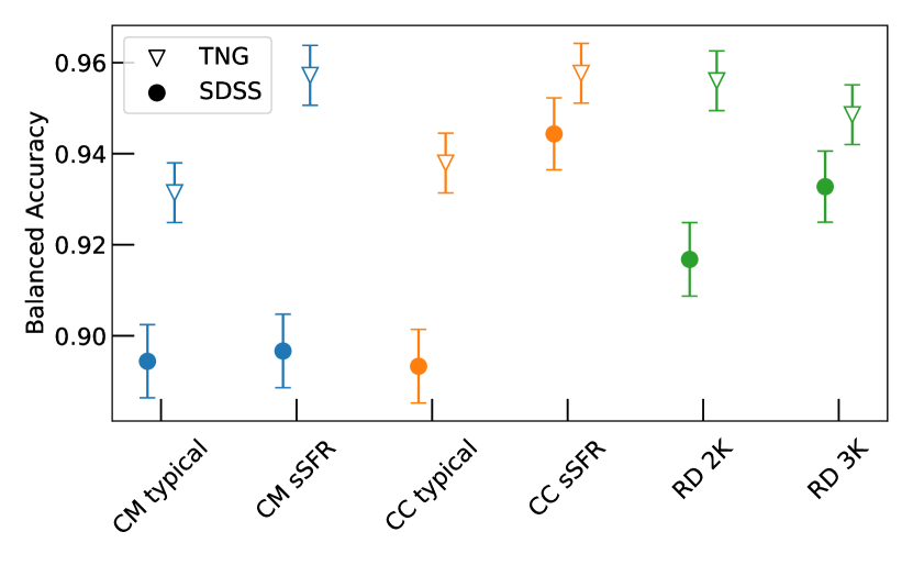
Figure 4: Balanced accuracy in selecting the quenched population of low-redshift ($z\doteq 0.1$) TNG and SDSS galaxies. Error bars generated from Poisson error estimates on each of the classification components. “CM” and “CC” methods draw hard cuts through color-magnitude and color-color spaces respectively, whereas the “RD 2$K$” and “RD 3$K$” methods use a Gaussian mixture model with $K=2$ and $K=3$ components respectively. The three-component dragons have tighter selections on the RS, yielding a lower false positive rate but a higher false negative rate, which for TNG galaxies results in a slightly decreased balanced accuracy.

To exemplify limitations of CM and CC hard-cut selections, we compare balanced accuracy in selecting the quenched population using hard cuts vs Gaussian mixtures for both the SDSS low-$z$ sample alongside the TNG sample, both at $z=0.1$ approximately.

Using methods from the literature, we make hard cut fits (labeled ‘typical’) in CM and CC spaces. Next we use sSFR values to optimize fits, drawing the hard cut lines which maximize balanced accuracies (labeled ‘sSFR’), giving a best-case scenario for hard cut selection methods. Finally, we compare these fits to Gaussian mixture fitting of the populations, i.e. using a Red Dragon approach for selecting the red sequence (labeled ‘RD 2K/3K’).

Figure 4 shows accuracies of these various selection types. For SDSS, even optimized CM selection typically incurs $\gtrsim 10\%$ error (i.e. $\sim 10\%$ of the RS and BC contain star-forming or quenched galaxies respectively) while optimized CC selection typically incurs $\gtrsim 6\%$ error, showing as did Figure 3 that two colors (CC space) work significantly better than one (CM space). Hard cuts in CM and CC spaces select the quenched population more accurately in TNG than in SDSS, largely due to its more pronounced GV (see appendix A), with a typical error of only $\sim 5\%$ by any selection method.

Gaussian mixtures (without any optimization from sSFR truth) perform generally on par with optimized CM and CC fits but have higher selection accuracy than CM and CC fits similarly ignorant of sSFR. Given a spectroscopic sample of galaxies, where sSFR values are known, Figure 4 shows that one could define hard cut selections of the RS which would have accuracies similar or superior to a GM selection of the RS. However, at redshifts where the RS & BC are not well defined from spectroscopy, or at any redshift where sSFR values are unknown, a GM would give superior selection of the quenched population.

4.1.2 Redshift continuity of quenched galaxy selection

Here we investigate Red Dragon’s accuracy in selecting the quenched population as a function of redshift. The SDSS mid-$z$ sample centers around the transition redshift of $z\sim 0.4$, where the 4000 Å break moves from $g$ band into $r$ band.

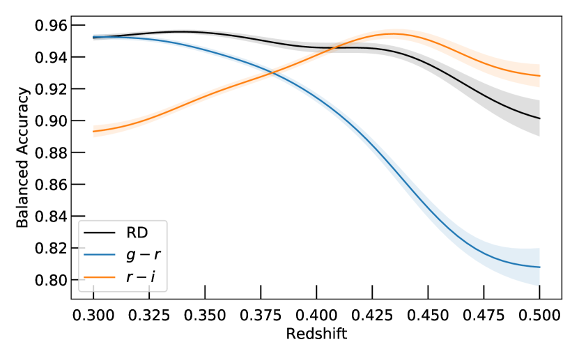
Figure 5: Balanced accuracy in selecting the quenched population of bright SDSS galaxies: Red Dragon (RD; black) performs similarly or superior to hard cuts in single colors. Bootstrap $\pm 1\sigma$ error shown with transparencies; these increase with redshift chiefly due to decreasing number counts (rather than from increased intrinsic scatter). Values localized by Gaussian kernel (width $\sigma_{z}=.02$).

Figure 5 compares accuracy in selecting the quenched population between Red Dragon and two (redshift-evolving) choices of single-color cuts for defining the RS. As the 4000 Å break passes from $g$ band to $r$ band near $z=0.36$ (thus affecting the values of $g-r$ and $r-i$), the ability of $g-r$ to select the quenched population wanes while that of $r-i$ waxes, as expected. If using single-color selection, $z=0.38$ would then be the best redshift to transition from selecting the RS with $g-r$ to selecting with $r-i$ (if your goal is to select the quenched population with greatest fidelity).

In comparison to these single-color selection methods, Red Dragon performs similarly to best-case single-band selection (within $3\sigma$), with vastly superior ($>6\sigma$) accuracy across $z=0.38$, the optimized transition redshift. We note here that the high-redshift side of the plot has significantly lower number counts, and lacks statistical power compared to the low-redshift side. If using single-color selection of the RS, optimal transition redshifts between colors are somewhat subjective. The initial calibration of the RS by RedMaPPer transitions from using $g-r$ to using $r-i$ at redshift $z=0.35$ (the 4000 Å transition redshift; also the point below which the survey is volume limited and above which is magnitude limited). However, they found that the redshift for which single-color richnesses $\lambda_{g-r}$ and $\lambda_{r-i}$ equaled their multi-color richness $\lambda$ was at redshift $z\doteq 0.42$ (see their Figure 28), so a reliable $\lambda_{\rm col}$ definition would use $z\doteq 0.42$ as a transition redshift. Neither $z=0.35$ nor $z=0.42$ match the single-color transition point highlighted by Figure 5 of $z=0.38$ (the redshift at which trading off from $g-r$ to $r-i$ maintains the highest quenched population selection accuracy). Since these redshifts each have sound reasoning for their use in defining a single-color RS selection, no universal transition redshift stands out. This leaves single-color RS selection transitions as messy at best, favoring the objectivity of multi-color analyses.

Red Dragon preserves accuracy in selecting the RS across redshift transitions while maintaining a continuous red fraction (by construction). This then evades the discontinuities inherent in swapping bands,continuously selecting RS galaxies with high fidelity.

4.2 Buzzard Flock analysis

Extending our analysis to a wider redshift range, we turn to the synthetic galaxy catalogs of the Buzzard Flock with the three primary colors of equation (2). After highlighting how fits interpolate across redshift (§4.2.1), we discuss how the RS definition varies as component count increases from two to four (§4.2.2).

The Buzzard universe is a statistical replica of a deep-wide galaxy survey built from galaxy color distributions measured as a function of local cosmic overdensity (Hogg et al., 2004). The ADDGALS method is trained empirically at low redshifts and extrapolated to high redshifts using a spectral energy distribution template approach (for details, see Wechsler et al., 2021). While the method reproduces well the counts and two-point clustering statistics of galaxies (DeRose et al., 2021), behaviors of the Buzzard universe at high redshifts are less rooted in observation than those at low redshift.

With a sample size of 94M galaxies (see table 1) we are able to extract precise estimates of all model parameters. However, the statistical errors shown below are lower limits, in that systematic variations caused by a different galaxy catalog construction method (see e.g. MICE (Carretero et al., 2015), cosmoDC2 (populated by GalSampler algorithm Hearin et al., 2020), etc.) remain to be investigated.

For RS mean and scatter, we compare to Hao et al. (2009) (SDSS catalogue) and Rykoff et al. (2014) (DES catalogue). Hao et al. (2009) fit SDSS data using an error-corrected GMM in $g-r$. With that selection for blue and red, mean colors as a function of $i$ band were measured along with scatters, all as functions of redshift. Rykoff et al. (2014) fit data using a multivariate error-corrected GM in the primary colors of $griz$ (see equation 2). Their algorithm iteratively selects the RS, measuring a slope of its color as a function of $z$ band, giving a redshift-continuous fitting across redshift much like Red Dragon. This method was then applied to DES Y3 data to provide an observed RS fit (E. Rykoff, private comm.). Both methods only fit the RS, so no information on weight nor any fits for the BC are available for comparison to Red Dragon.

4.2.1 Redshift Evolution of Two-Color GMM Components

This section details a fitting of the evolving GMM parameters across redshift for Buzzard photometry. The galaxy sample is magnitude-limited using the redshift-evolving cut of $0.2\,L_{*,i}(z)$ from Rykoff et al. (2014) within the redshift range $0.05<z<0.84$. The galaxies are divided into narrow cosmological redshift bins of width $0.025$, resulting in counts per redshift bin of 60k to 7.5M galaxies. Red Dragon is run on 50 bootstrapped samples of size $10^{4}$ (undersampling for the sake of speed, efficiency, and easing computational burden); the resulting median parameters $\theta(z_{i})$ and $\pm 1\sigma$ quantile range for each bin are shown in the figures below. The discrete redshift parameters are then interpolated using KLLR with a Guassian kernel of width $\sigma_{z}=0.02$, shown as lines in the figures below.

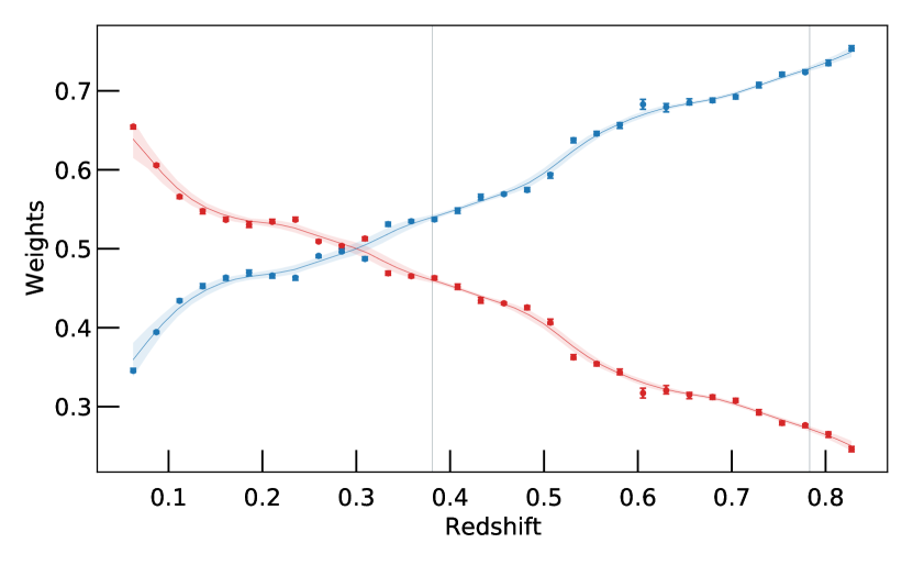
Figure 6: Component weight for RS (red) and BC (blue) as a function of redshift for the Buzzard flock. Points show parameter fits from individual redshift bins with bootstrap errors shown as error bars. Fit line interpolation smoothed with KLLR (Gaussian kernel width $\sigma_{z}=0.02$) with uncertainty in fit shown as transparencies about the line. Vertical grey lines indicate transition redshifts of the 4kÅ break from Table 2.

Component Weights.

A variety of deep observations of the real universe indicate that star formation rates per unit baryon mass were much higher in the past (Madau et al., 1996; Connolly et al., 1997; Madau & Dickinson, 2014). Astrophysically speaking, while the Butcher-Oemler effect of reddening over time (Butcher & Oemler, 1978) applies primarily to galaxy clusters, the entire population of galaxies ages and tends to redden as a whole. Quenching is nearly a one-way process for galaxies (many models ignore the reverse direction entirely, e.g. de la Bella et al., 2021), implying that the only way to decrease red fraction over time is to create new blue galaxies. Since the peak of cosmic noon was at $z\sim 1.9$ (Madau & Dickinson, 2014), galaxy samples below this redshift should redden over time. We therefore expect Red Dragon, when applied to Buzzard, to extract a RS weight that declines with increasing redshift (i.e. the population becomes bluer with increasing redshift).

In good agreement with this expectation, Figure 6 shows that the RS weight consistently decreases with redshift, ranging from roughly 70% at redshift $z=0$ down to 25% at the highest redshift of $0.84$. Since the red fraction is highly luminosity dependent (as discussed in appendix D), one should rememeber that the weight reported here represents a weighted average of all galaxies above $0.2L_{\ast}(z)$, which will be dominated by magnitudes near the cutoff. Choosing a brighter magnitude cutoff would uniformly raise the RS weights, and vice-versa.

The bootstrap uncertainties are typically quite small, but there is an increase near $z=0.6$ (seen somewhat if figure 7 and especially in the correlations of 8). Here, rather than giving slight variations around a single fit as at earlier redshifts, pyGMMis at this redshift debates between two distinct fits: one with wider scatter (and low correlation) and one with narrower scatter (and high correlation), each of which having differing RS weight. These two modes exist in very few of the previous bootstrap realizations, but near $z=0.6$ make up roughly half of the fits. Since Bootstrap resampling yields two discrete modes, the overall uncertainty is relatively large compared to single-mode redshift bin fits.

Mean Colors.

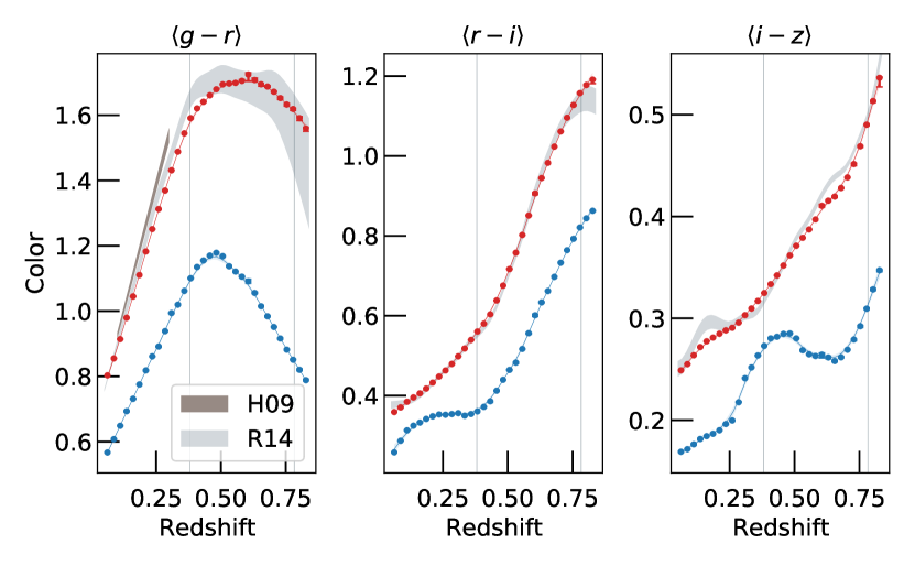
Figure 7: Points show mean colors for each GMM component (RS & BC) for Buzzard galaxies, using the same coloring as Figure 6. RS mean measurements from Hao et al. (2009) (SDSS, $g-r$ only) and Rykoff et al. (2014) (DES Y3, all colors) are shown for comparison. Due to their dependence on magnitude, we present ranges from $0.2\,L_{*}$ (the magnitude limit of Buzzard; lower edge of transparencies) up to $L_{*}$ (upper edge of transparencies). respectively.

Figure 7 shows the redshift evolution of the mean colors of the two components. The three panels each show measured BC and RS means in different colors with comparisons to observations in shades of grey (Hao et al. (2009) only fit $g-r$ at low redshift). Since these observations were magnitude dependent (whereas the Red Dragon fitting of Buzzard is magnitude independent), mean colors between $L_{*}$ (upper bound of transparency) and at $0.2\,L_{*}$ (limiting luminosity of Buzzard galaxies; lower bound of transparency) are shown for comparison. Because over two-thirds of Buzzard galaxies fall between these two limits, we expect our mean color fitting to also be between these bounds as well. However, the Buzzard photometry differs from photometry input for the comparison observations, so the fits will differ somewhat. Note that each color has different vertical scaling: $\langle g-r\rangle$ spans the largest range while $\langle i-z\rangle$ spans the smallest range, exaggerating its features.

At transition redshifts (see Table 2), the slope of mean color with respect to redshift changes rapidly, necessitating narrow redshift analysis bins and careful fitting. Mean colors for both RS & BC follow a general shape of rising as the 4000 Å break enters the color’s minuend, then falling as the break enters the color’s subtrahend, as expected.

Compared to observed mean colors, Buzzard shows a bluer red sequence for $z\lesssim 0.45$ in $\langle g-r\rangle$, albeit by a small margin. Comparing to the Rykoff et al. (2014) method, deviations from observations are consistently $<0.034~{}{\rm mag}$ (only $0.005~{}{\rm mag}$ deviant on average). For $z\gtrsim 0.45$, colors vary more with magnitude (steeper RS slope in CM space), such that Buzzard mean colors land between the $0.2\,L_{*}$ and $L_{*}$ observations.

If the mean spectra of RS and BC galaxies had no time evolution, then the same general shape of each curve in figure 7 should appear for each color, shifted by roughly $\Delta z=.4$ (and vertically scaled somewhat for differences between bands). We see this to some extent, e.g. with the rising of the RS $\langle g-r\rangle$ in $z|[0,0.4]$ mirroring the rising of the RS $\langle r-i\rangle$ in $z|[.4,.76]$. Similarly, the BC bump in $\langle i-z\rangle$ at $z\sim 0.5$ mirrors the $z\sim 0.1$ BC bump in $\langle r-i\rangle$ (the vertical scaling difference between the axes belies their similarity). As our analyses extended to higher redshifts in future work, we will find similar universal features or find time variation in RS and BC populations.

Color Covariance.

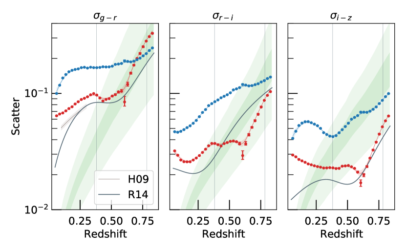
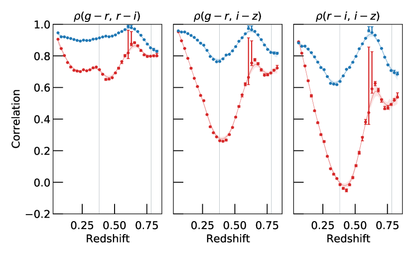
Figure 8: Intrinsic color scatter (upper panel) and correlations between colors (lower panel). Green transparencies give one and two-sigma quantile distributions of photometric color errors in Buzzard. Coloring of components and interpolation as detailed in Figure 6; comparison to observations as in Figure 7.

The top row of Figure 8 shows the redshift evolution of the intrinsic scatter in each color for both GMM components. Showed also are the fits from observations in grey (as before but without magnitude dependence) as well as $\pm 1\sigma$ and $\pm 2\sigma$ median quantiles for color errors, shown as green transparencies. The bottom row of Figure 8 shows intrinsic correlations between colors inferred from the covariance matrix, giving $\rho(g-r,\,r-i)$, $\rho(g-r,\,i-z)$, and $\rho(r-i,\,i-z)$ from left to right.

In accordance with expectations, at redshifts where the color’s minuend contains the 4000 Å break, the RS has significantly lower scatter than the BC (by a factor of $\sim 2$), indicating a tighter population. Due to an increase of photometric errors at higher redshifts (as shown by the green transparencies), it’s difficult to accurately constrain population scatters. Beyond redshift $z\sim 0.4$, the median photometric error exceeds the intrinsic RS scatter, making it difficult to measure.

Compared to observed RS scatters, Buzzard scatters are generally wider by a factor of 1.5 (consistently within a factor of three above or below). Running of the RS mean color with magnitude means that a magnitude-ignorant fitting of the population scatter would find larger values than a magnitude-cognizant model, so Buzzard’s generally wider scatters are expected. Since Rykoff et al. (2014) only fit the RS, a Red Dragon fitting of the RS (which also accounts for and fits the BC) is not guaranteed to identify the same exact RS. This will be further investigated in our papers to come, analyzing DES data.

While measures of the RS scatter in various colors are available in the literature (Hao et al., 2009; Rykoff et al., 2014), to our knowledge there is no published work on measuring the intrinsic scatter of the BC nor covariance among primary (or otherwise) colors for RS and BC galaxies. If this is correct, the BC scatter and full color covariance as a functions of redshift constitute empirically unexplored territory. Our Buzzard measurements are then establishing a first estimate of these quantities, albeit one more likely to reflect that of the true galaxy population at low redshift than at high redshift.

Though intrinsic color correlations within each of the RS and BC are expected to be $\gtrsim 90\%$ (Rykoff et al., 2014), the GMM fitting of Buzzard usually has lower (and occasionally even has negative) correlations between colors. Since the simulated photometric errors in Buzzard were of similar order to the RS scatter for $z\gtrsim 0.4$ (see the green transparencies of Figure 8’s upper panel), these correlations represent more so relations between photometry than intrinsic correlations within the RS. In comparison, the BC has a width larger than the photometric error at all but the highest redshifts, and accordingly, we see high correlations, around 80% to 90% across redshift.

These fits show that Red Dragon can map out the RS and BC to high redshift (spanning across multiple transition redshifts), continuously parameterizing important aspects of each population. As future studies create more complete samples of galaxies to higher redshifts, Red Dragon will be able to detail population characteristics smoothly across even wider redshift ranges.

4.2.2 RS robustness to component count

Here we investigate how Red Dragon identifies the RS in models with more than two components. On adding additional components to a Gaussian mixture model, one generally expects (1) a reduction in weight of each component, (2) a reduction in scatter, and (3) a shift of the means as the new component displaces the old. Figure 9 compares red fraction, RS mean $g-r$ color, and RS $g-r$ scatter for varying component counts $K=\{2,3,4\}$ in the Buzzard flock. We find that while the RS has a relatively consistent mean and scatter on adding components, the RS is subdivided between components at low redshifts, resulting in a drastically different weight for the reddest component.

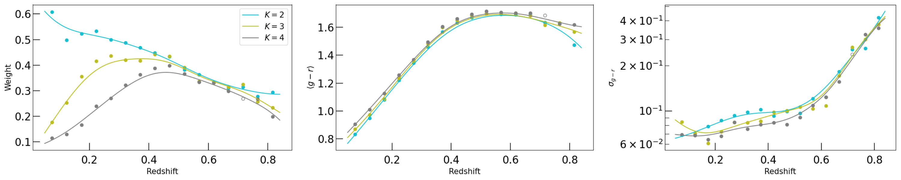
Figure 9: RS fit variation between component count K, shown for photometric color ($g-r$). Left: Red fraction decreases significantly with the addition of more components below $z=0.4$, but for higher redshifts, weight varies less than $5\%$ (typically by $\sim 1\%$). Middle: Mean RS color varies by less than $0.05~{}{\rm mag}$ on adding a component (typically by $\lesssim 0.01~{}{\rm mag}$). Right: Scatter in the RS decreases with the sub-division of additional components, on average by $<4\%$, consistent to less than a factor of $1.5$ across all redshifts.

We find good consistency in red fraction (leftmost plot of Figure 9) for $z>0.4$, with only minor reduction in weight with added components (typically order 1%, consistently $<5\%$). For $z<0.4$, we see a severe reduction in red fraction of the reddest components for $K=3$ and $K=4$, due to the RS being subdivided into multiple components.

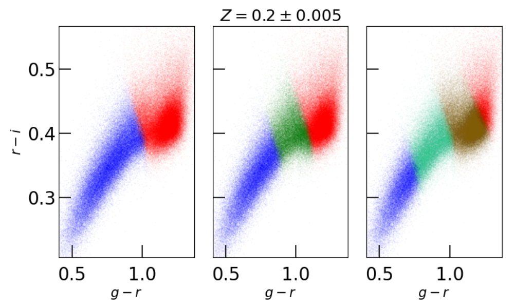
Figure 10: Red Dragon population characterization for Buzzard galaxies in the thin redshift slice $z=0.2\pm 0.005$ for different component counts. Left: $K=2$, Middle: $K=3$, Right: $K=4$. With four components, the RS and BC are further subdivided into bluer and redder components.

At a single redshift slice ($z\approx 0.2$), Figure 10 shows this sub-division of the RS for each component count. On the same axes of $g-r$ vs $r-i$, the thin sample of galaxies are colored by component classification for $K=2$ to $K=4$ component mixtures. Addition of components primarily splits populations into bluer and redder sub-populations, but the fraction of star-forming or quiescent galaxies belonging to each population varies strongly with changing $K$ values.

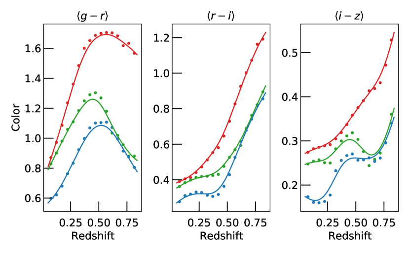
Figure 11: Mean color values for all three components of a $K=3$ fitting of Buzzard photometry. The red lines consistently track a quiescent population and the blue lines consistently track the star-forming population. The green component moves from clearly matching the star-forming population at high redshifts to clearly matching the quiescent population at low redshifts.

Figure 11 illustrates this sub-division in mean colors $\mu_{\alpha}(Z)$ for the $K=3$ model across redshift, similar to Figure 7: the middle component (green line) matches the BC at high redshifts, but matches the RS at low redshifts. Though this could be characterizing galaxy evolution from BC to RS, it may be a statistical artifact, where the RS is more non-Gaussian at low redshifts than at high redshifts, as compared to the BC. Without data on sSFR and galaxy evolution in Buzzard, it’s difficult to say. If using $K>2$, one must be careful in labeling the RS, since the quiescent population may be split between components.

Besides weight, we find excellent consistency in the other GM parameters. Mean color changed on average by $\lesssim 0.01~{}{\rm mag}$ on adding a new component (consistently less than $0.05~{}{\rm mag}$; see Figure 9, center plot). Scatter reduced on average by $<5\%$ with each added component (consistently less than $<33\%$; see Figure 9, rightmost plot). Correlations varied by less than 12% on average. Though the populations are consistently characterized, single components may not consistently correspond to the same population; middle components may at one redshift characterize the quiescent population but at another characterize the star-forming population.

As discussed earlier (see §3.2.3), the optimal count of Gaussian components to use in modeling depends on the dataset; increased non-Gaussianity requires more nuanced modeling. Despite non-Gaussianities in our datasets, the two-component model still aptly characterizes the galaxy population. Adding extra components must be done with care due to complexities in modeling and interpretation.

5 Conclusions

We present Red Dragon, a new method for galaxy population characterization, which evolves Gaussian mixture models in the space of broad-band optical colors across redshift. With the red sequence of quiescent galaxies as a target population in both observed and simulated galaxy samples, we demonstrate the method’s ability to identify the quenched population with similar accuracy to previous approaches but with smoother continuity across redshift (in addition to characterizing the BC).

Jumping from using one color alone to another as a RS selector (e.g the transition from $g-r$ to $r-i$ near $z=0.4$) gives an inherent discontinuity in red fraction $f_{R}(z)$ or in accuracy of selecting the quenched population. Since Red Dragon interpolates Gaussian mixture parameters across redshifts in multi-color space, the resulting characterization of galaxy photometry yields a continuous red sequence definition (thereby resulting in a continuous red fraction). If metrics such as richness and red fraction are to be broadly interpretable across wide redshift spans, we must move beyond discontinuous single-color selection of the RS.

By construction, Red Dragon also offers a new way to explore RS, GV, and BC photometric behavior through its explicit fits to population weight, mean color, scatter, and correlation between colors. This fitting allows investigations into the photometric sub-populations of galaxies, such as fraction of transitioning galaxies as a function of redshift, or the evolution of mean color and scatter of blue cloud galaxies.

Fitting the population with Gaussian mixtures results in similar or superior selection of quenched galaxies as optimized color–magnitude (CM) or color–color (CC) selections (see figures 3 and 4). Simple CM and CC selections lack information gained from the other colors (corresponding to properties such as dust, age, and metallicity; see section 2.3), which information would help disentangle degeneracies between red sequence and blue cloud in photometric space. Though an optimized cut in CC space can select the quenched population with similar accuracy to that of a GMM, such a selection only works well for a limited redshift span. To preserve accuracy across larger redshift spans, interpolating Gaussian mixtures in multi-color space serves as a straightforward and natural way to extend the RS to higher redshifts.

We note here that in addition to extending deeper into the infrared (towards $Y$, $J$, $H$ filters), higher-energy wavelengths could also be added. Even X-ray data show differences between RS and BC (Comparat et al., 2022), so pan-chromatic analyses of populations would certainly improve characterization of the RS and BC, better distinguishing the two populations.

A continuous RS definition across wide redshift spans will be critical as future galaxy surveys push deeper and fuller into the redshift regime. The RS has already been detected beyond $z=2$, with evidence for a quenched population out to $z<2.5$ (Kriek et al., 2008; Williams et al., 2009; Gobat et al., 2011; Golden-Marx et al., 2021). Future telescopes such as Euclid and the Nancy Grace Roman Space Telescope will provide NIR-band observations of galaxies out to high redshifts, measuring the 4000 Å break for high-$z$ galaxies. Modeling of the RS continuously beyond $z=1$ (and eventually $z=2$) will be critical moving forward, allowing for meaningful interpretation of measures such as red fraction or richness.

Data Availability

The current iteration of Red Dragon is available on Bitbucket at wkblack/red-dragon-gamma. Methods used in this analysis are also available at wkblack/red-dragon on Bitbucket. Data from SDSS and TNG are publicly available on their respective servers.

Appendix A SDSS vs TNG color distribution

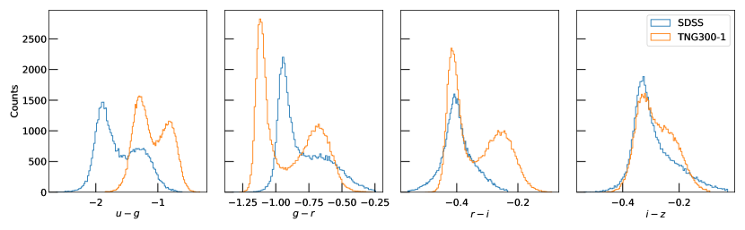
Figure 12: Comparative number densities in SDSS (blue) vs TNG (orange; simulated errors) for primary colors (both at $z\doteq 0.1$). Note that for each color, TNG has far more drastic valleys between RS and BC than SDSS (which only visibly shows a valley for $u-g$ here). Thus, any selection of RS and BC in TNG will be far cleaner than in SDSS.

Though photometry between SDSS and TNG have similar mean colors, the distinctness of RS and BC differ significantly between the two datasets. Figure 12 shows histograms of color distributions for TNG as compared to SDSS. Errors on TNG magnitudes were simulated to match SDSS trends, as detailed in table 4.

band	log slope $\alpha_{x}$	intercept $\epsilon_{0,x}$
$u$	$0.235\pm 0.001$	$-1.742\pm.0019$
$g$	$0.185\pm 0.001$	$-2.212\pm.0004$
$r$	$0.187\pm 0.001$	$-2.182\pm.0004$
$i$	$0.195\pm 0.001$	$-2.097\pm.0006$
$z$	$0.246\pm 0.001$	$-1.619\pm.0011$

Table 4: Log slope $\alpha_{x}$ and intercept $\epsilon_{0,x}$ of SDSS typical band errors, fitting $\log_{10}\epsilon_{x}=\alpha_{x}(m_{x}-m_{\rm ZP})+\log_{10}\epsilon_{0,x}$ for each band $x$, with magnitude zero point $m_{\rm ZP}=17.3$. Note that these are fairly close to error $\epsilon\propto L^{-1/2}$, which implies $\log_{10}\epsilon=.2\,m_{x}+C$.

Even with these added errors, TNG displays far clearer separations between RS and BC than SDSS. While SDSS only has a visible valley for $u-g$ (in the primary colors), TNG shows significant valleys for all but $i-z$ (the noisiest bands, furthest from the 4000 Å break at this low redshift).

The stronger dichotomies of TNG made selection of the RS far cleaner for TNG than for SDSS. This explains the vast increase in constraining power in Figure 4 from SDSS to TNG, and the relatively consistent accuracy across selection methods.

Appendix B Galaxy Spectra Astrophysics

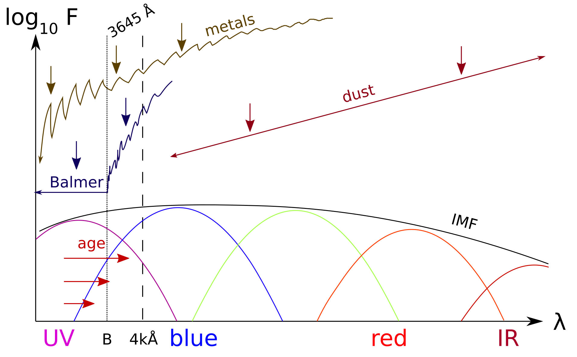
Figure 13: Summary cartoon of main astrophysical effects determining galaxy colors. Stars provide the vast majority of optical light, with short-lived blue giants providing the majority of short-wavelength light and longer-lived red giants providing the majority of longer optical wavelengths. The overall shape of the emission spectrum depends on both the stellar initial mass function (IMF) and the star formation history (SFH). Main sequence stars redden with age, with blue giants aging the fastest ($\tau_{\rm MS}\propto M^{-2.5}$). Thus, old galaxies emit less short-wavelength (optical) light. Primary sources of absorption include dust reddening and line absorption. Dust presence causes Rayleigh scattering: the preferential scattering of short-wavelength light (intensity $I\propto\lambda^{-4}$). Such scattering reddens the overall spectrum, which can be clearest observed in the post-break slope. Though this effect is somewhat degenerate with age and metallicity, both age and metallicity reduce low frequencies exponentially more, whereas dust effects are linear in log flux. The many absorption lines of various metals convene around (and especially at wavelengths shorter than) 4000 Å, resulting in a blanket of absorption. Galaxies with identical $\tau Z^{3/2}$ (i.e. $\Delta\,{\rm age}\,/\,\Delta\,{\rm metallicity}=3/2$) have virtually identical optical colors (Worthey, 1994), so the two effects are highly degenerate. In contrast to the smoother effects of age or metallicity, hydrogen line absorption asymptotes towards 3645 Å from above (with shorter wavelengths both fully ionizing hydrogen atoms and imparting a surplus kinetic energy kick). This convergence of the Balmer series results in a sudden drop in emissions—sharper than that of line blanketing. Thus the IMF / SFH, age, dustiness, and metallicity of galaxies all play a role in determining their overall spectrum and membership of the RS / BC.

This section summarizes the main astrophysical effects which determine spectral shape for galaxies at optical wavelengths. Generally, the most striking spectral difference between RS and BC is the galaxy’s quenched status, as measured by the strength of D4000. However, other factors help separate RS from BC, such as galactic dust content, metallicity, or age. These secondary factors affect colors beyond just the color used to measure D4000, so multi-color analysis serves to better distinguish the RS from the BC than a raw measurement of D4000.

Dust plays a substantial role in altering a galaxy’s position in multi-dimensional photometric color space. Due to Rayleigh scattering, shorter wavelengths scatter easier, with scattering intensity $I\propto\lambda^{-4}$. Thus, the presence of dust depresses bluer wavelengths, inflating the overall spectrum slope $d\log F/d\lambda$, reddening all photometric colors. Therefore, the post-break slope (blue–infrared slope in rest frame) correlates highly with dust content. Furthermore, once galaxies are stripped of their dust, insufficient material exists for stellar creation, so star formation rates decline.

Age and metallicity also redden galaxy spectra. As stars age, they leave the stellar main sequence and become red giants. When galaxies as a whole age, they therefore also redden. Age then affects the spectrum similarly to dust, reddening overall but particularly so near the break (Worthey, 1994). Stars produce metals with age, which cause increased amounts of line blanketing. This blanketing causes widespread reddening, particularly near 4000 Å and shorter (ibid.). As mentioned earlier, since the Balmer break (asymptotically approaching 3645 Å) is caused by hydrogen abundance while line blanketing (approximately around 4000 Å) is caused by stellar metallicity, the two effects result in different spectrum curvatures about the break. A ratio of the two effects relates to the metallic abundance ratio [Fe/H], so curvature correlates with metallicity (see also Chalonge & Divan, 1977, Fig. 2). Though spectrum curvature cannot be encapsulated in a single color, paired colors can capture spectrum curvature to some extent.

Figure 13 shows a graphical summary of these main astrophysical effects which determine optical–IR galaxy spectral shape. Of primary relevance are the effects of the Balmer break (at 3645 Å), dust (reddening the entire spectrum), age (most noticed as a reduction at the blue end of the spectrum), and metallicity (causing line blanketing, especially $\lesssim$ 4500 Å; see Lejeune et al., 1997).

Comparison to BCD stellar classification scheme

Incidentally, the main effects affecting galaxy spectral shape (star formation, dust presence, age, metallicity) correspond well with the BCD stellar classification scheme (Barbier & Chalonge, 1941). The BCD system gives a more precise (3D, continuous) stellar classification model than the common MK system (2D, discrete). Its three distinguishing parameters measure

1. $D$, the ratio of spectrum intensities spanning the 4000 Å break;

2. $\phi_{b}$, the blue–violet post-break spectrum slope; and

3. $\lambda_{1}$, the midpoint location along the drop.

Larger values of $\lambda_{1}$ indicate a smoother break, implying more line blanketing than Balmer line absorption, thus correlating well with metallicity; more directly, the difference between the NIR slope $\phi_{n}$ (pre-break, ca. 3500 Å) and blue–violet slope $\phi_{b}$ (ca. 4000–4600 Å) shows strong correlation with metallicity (see Chalonge & Divan, 1977, Fig. 2). As galaxy luminosities arises from stellar luminosities, it should be no surprise that similar distinguishing markers should be sought after for both stars and galaxies.

Appendix C Optimal Number of Components

In this section, we consider the optimal number of components to characterize the SDSS/low-$z$ galaxy population, as determined by the Bayesian Information Criterion (BIC; Schwarz, 1978):

$$\mathrm{BIC}\equiv k\ln(n)-2\ln(\widehat{L})$$ (10)

BIC penalizes large parameter counts $k$ (with additional weight for increased number of data points $n$) while rewarding increased maximum likelihood $\widehat{L}$, such that lower BIC values indicate a superior model. The relative likelihood of two models is proportional to $\exp(-\Delta{\rm BIC}/2)$, so values of $\Delta{\rm BIC}\gtrsim 10$ indicate significant evidence for model superiority. Since only relative BIC matters, we measure here $\Delta{\rm BIC}_{K}\equiv{\rm BIC}_{K}-\min({\rm BIC}_{K})$: the value of BIC (for any component count $K$) relative to the minimum BIC (across all $K$).

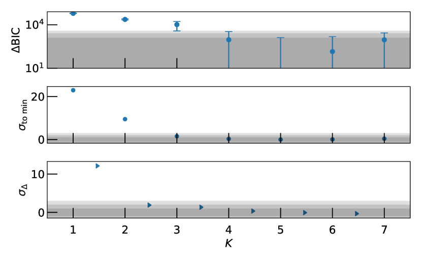
Figure 14: Bayesian Information Criterion (BIC) information for SDSS low redshift sample ($z=0.1\pm 0.005$), evidencing the limited gains of $K>3$ Gaussian mixture components. Error bars estimated from bootstrap resampling. Grey bands indicate $\pm 3\sigma$ range for minimum BIC. All off-screen errorbar tails are negative, i.e. below the minimum BIC’s mean value). Top: BIC relative differences (i.e. ${\rm BIC}-\min({\rm BIC})$). Though a decrease in BIC $>10$ indicates significant evidence for an improved model, bootstrap errors on BIC measurements reveal insignificant gains, especially at higher component counts. Mid: Sigma from each point to the BIC minimum. Bot: Significance of BIC gain on incrementing component count.

Figure 14 shows our analysis of BIC for the SDSS/low-$z$ sample. The upper panel gives BIC values relative to the minimum BIC (at $K=5$), the middle panel shows the significance of the differences in those BIC values, and the lower panel shows the incremental gain in significance on increasing $K$. In each panel, the error of the $K=5$ model is shown for $\pm 3\sigma$ as transparencies. These plots aid in choosing a number of components $K$ that both optimizes fitting of the galaxy population while avoiding overfitting.

Though the upper panel shows that the SDSS/low-$z$ three-component model ($K=3$) has $\Delta{\rm BIC}\doteq 10^{4.01}$, the middle panel shows that accounting for uncertainty at both $K=3$ and at $K=5$ (the absolute minimum) implies that the two are $<2\sigma$ different—the BIC of the $K=3$ model is indistinguishable from the measured minimum, statistically speaking. From a BIC standpoint, there is no statistically significant reason to use $K\geq 4$ for this dataset. This highlights the importance of calculating error bars on BIC values; while such a high $\Delta$BIC would indicate overwhelming support of a five-component model over a three-component model, the errors on each BIC value reveal the actual insignificance of their relative $\Delta{\rm BIC}$.

One can also compare BIC gains incrementally: as we add an additional component, how significantly do we decrease BIC? If adding a component doesn’t significantly decrease BIC, it may not be worth the added complexity. Though moving from one component to two gives a $>12\sigma$ improvement in BIC, moving from two to three components only improves BIC by $<2\sigma$ (with further increments yielding even smaller gains). Even though the $K=2$ model has a BIC significantly ($\sim 10\sigma$) above the absolute BIC minimum, incremental gains beyond $K=2$ are insignificant. This again favors models with $K<5$, despite $K=5$ being the BIC minimum on average. Based on the above analysis for this particular dataset, we advise using either $K=2$ or $K=3$ components to model the distribution of galaxies.

Though BIC accounts for the cost of extra parameters, it doesn’t account for human usefulness directly; models with fewer components are more easily analyzed whereas larger component counts become increasingly difficult to consistently model and interpret across redshift.

The spirit of BIC is to maximize likelihood while minimizing complexity: a model should use the lowest component count possible while still achieving significant decreases in BIC. To this end, we suggest using a two or three-component model of galaxy colors. Using a two-component model has the upside of easier interpretation. While two Gaussian components unambiguously model the RS and BC across all redshifts, even a three-component model can give rise to significant ambiguity. As discussed in section 4.2.2, while the third component sometimes models a middle population (galaxies transitioning from BC to RS) at other times it models the larger scatter surrounding the RS and BC (modeling kurtosis of the population). Extra components beyond three lack intuitive explanation from the underlying astrophysics and lack statistical power to increase model favorability. Practically speaking, larger numbers of evolving components are far trickier to map between redshifts. Continuous modeling of four components is taxing at best, with meaningful interpretation of each component across all redshifts a tricky issue. Caveat emptor. For simplicity of discussion and comparison, we employ a two-component model for our results section as a minimum-use case.

Appendix D Magnitude trends in Buzzard

Here we investigate trends of magnitude running as found in Buzzard. Though running of parameters $\theta$ with magnitude is statistically significant (section D.1), slope of mean color relative to the scatter of the populations was relatively small (section D.2), so differences in selection were relatively minimal (section D.3). Magnitude trends had the largest effect for dimmer galaxies, resulting in $\mathcal{O}(10\%)$ differences in selection.

D.1 Strength of linear trend

To give a general feel on the significance of magnitude running in Buzzard, we let each GMM parameter run linearly with magnitude and analyzed several redshift slices. First results show that brighter galaxies are more likely red ($df_{R}/d{m_{i}}\approx-0.13$, such that faint galaxies are almost always BC members), with the degree of redness increasing gradually with luminosity ($d\mu_{(g-r),\,{\rm RS}}/d{m_{i}}\sim-0.04$), more significantly so for the BC ($d\mu_{(g-r),\,{\rm BC}}/d{m_{i}}\sim-0.1$). The RS scatter increases at fainter magnitudes ($d\sigma_{(g-r),\,{\rm RS}}/d{m_{i}}\sim z/3$), especially at higher redshifts, but the scatter of BC galaxies doesn’t show significant linear evolution with magnitude. While $f_{R}$ runs near linearly with magnitude at a fixed redshift, $\mu$ and $\log\sigma$ have more quadratic or cubic running with magnitude (at fixed redshifts)—their fitting deserves more attention in the future, to best quantify the running of Gaussian mixture parameters with magnitude and redshift.

Red fraction varied more significantly with magnitude compared to the other parameters, with a roughly linear evolution with magnitude and redshift:

$$f_{R}(m_{i},z)\sim-.13(z+.5)(m_{i}-23.1).$$ (11)

This shows that fits gave null $f_{R}$ for $m_{i}>23.1$, i.e. only bright red galaxies truly belong to the red sequence—dim red galaxies belong to the blue cloud. Over Buzzard’s redshift range of $z|[.05,.75]$, this means the red sequence went from 0 to 100% across some 6–14 magnitudes, or a factor of $10^{2.5}$–$10^{5.6}$ in luminosity. Thus a linear fit to the RS catches the most BC members at faint magnitudes.

Allowing $f_{R}$ to run with magnitude could produce a more natural definition of the RS than traditional luminosity-limiting definitions of richness $\lambda$. Since faint galaxies rarely belong to the RS (while the brightest galaxies nearly always belong to the RS), a negative value of $df_{R}/d{m_{i}}$ gives an inherent cutoff to the RS (as compared to the contrived cutoff of e.g. $L>0.2\,L_{*}$ or $m<m_{*}+1.75$). Defining RS galaxies in such a way would correspond better to the underlying photometric distribution than defining the RS with hard magnitude cuts, potentially improving its power as a mass proxy and its universality across redshift.

D.2 Shift of mean color relative to RS width

Though the RS may have a statistically significant shift in mean color, it may not significantly change selection of the RS by Gaussian mixture if that running is small compared to the width of the RS. To measure this, we use the metric $\varsigma$ to quantify slope of the RS relative to its scatter:

$$\varsigma\equiv\frac{d\langle\mu_{a}\rangle/dM_{b}}{\sigma_{a}}$$ (12)

(for color $c_{a}$ and magnitude $M_{b}$; the magnitude may be any—our three fits use $M_{r}$, $M_{i}$, and $M_{z}$).

For a sample of $0.2\,L_{*}$ limited galaxies with luminosities following a Schechter function (with $\alpha|[-1.5,-1]$), $3\sigma$ worth ($>99.7\%$) of its galaxies fall in a magnitude spread of $\Delta{\rm mag}<3.3$ and $5\sigma$ worth ($>99.9999\%$) of its galaxies fall in in $\Delta{\rm mag}<4.4$. Thus the shift in mean color generally moves less than four magnitudes. Using the $\pm 2\sigma_{\rm RS}$ definition of RS width from Hao et al. (2009), we can then take $4\sigma$ as the distance needed to move such that the RS radically shifts with magnitude. These two factors of four essentially cancel out, leaving $\varsigma$ as a unitless metric for significance of RS running. If $|\varsigma|<1$, the magnitude variation of the RS mean color is completely within the typical scatter of the RS, but if $|\varsigma|>1$, then the RS mean color moves beyond the typical scatter of the RS.

We measured $\varsigma$ values from SDSS data Baldry et al. (2004), the Buzzard flock, and a redMaPPer Rykoff et al. (2014) fit of the DES Y3 RS. Each of the three datasets had typical values of $|\varsigma_{\rm RS}|\lesssim 0.5$ and for all cleanly measured cases (low-magnitude fits on Buzzard were questionable) had $|\varsigma_{\rm RS}|<1.3$, implying that in nearly every case, the running of the RS mean color was small compared to its width. This implies that it takes many magnitudes to significantly shift the mean RS color, relative to its intrinsic scatter. Therefore, characterizing the RS in a magnitude-ignorant way will still properly select galaxies.

D.3 Similarity in selection

Though including magnitude running of GMM parameters would better represent the photometric population, the extra dimensionality of running with magnitude makes fitting more of a nightmare, and doesn’t drastically alter selection.

Though the current version of Red Dragon doesn’t include magnitude running, there are a few workarounds, if you’re hell-bent on including its effect. 1) You can slice your data by magnitude and run Red Dragon to characterize a bright vs dim sample of your galaxies, then interpolate between (or simply bin using) the two fits to estimate $P_{\rm red}$ for individual galaxies. 2) If working with a relatively thin redshift slice, you can set in the code Z=m_i, i.e. let Red Dragon measure and interpolate across magnitude rather than redshift. We use this latter method to measure similarity in selection between magnitude-running and redshift-running versions of Red Dragon.

At several thin redshift slices (for $z[.1,.7]$), we measured $P_{\rm red}$ differences between the color-only and magnitude-running dragons. In binary selection, these two dragons resulted in about 5% opposing characterization (i.e. 5% of galaxies were characterized as RS instead of BC or vice versa) with a balanced accuracy of about 95% (between magnitude-running dragons and redshift-running dragons; not an accuracy of selecting the quenched population). Looking at $\Delta P=(P_{\rm red,mag}-P_{{\rm red},z})$, we found that though about $\sim 7\%$ of galaxies had $|\Delta P|\gtrsim 0.25$, less than about 1.5% of galaxies had $|\Delta P|\gtrsim 0.50$ (so few galaxies had significantly different characterization). There was approximately 12% scatter off $\Delta P=0$. So while the effect of running with magnitude is notable, it can be ignored without much loss.

Magnitude matters most when you’re uncertain of redshift, but the current version of Red Dragon is designed for clusters, where you have very good redshift estimates. For the current iteration of Red Dragon, the algorithm remains magnitude-ignorant, solely using colors to distinguish RS from BC.

Appendix E Redshift selection

To avoid overwhelming pyGMMis, galaxies are chosen probabilistically (with replacement, allowing for bootstrap analyses). If redshift errors are supplied, then probability of selecting a given galaxy is weighted by its chance of being in a given redshift bin. Assuming Gaussian errors, the probability of some value $\mu\pm\sigma$ lying in interval $(a,b)$ is

$$P[(\mu\pm\sigma)\in(a,b)]=\frac{1}{2}\left|\operatorname{erf}\left(\frac{b-\mu}{\sqrt{2}\,\sigma}\right)-\operatorname{erf}\left(\frac{a-\mu}{\sqrt{2}\,\sigma}\right)\right|.$$ (13)

So we select galaxies randomly from the full sample, weighted by that probability.

If redshift errors are not available, then we randomly pick $N$ galaxies (with replacement, allowing for bootstrapping) within the desired redshift interval.

Appendix F Excluding data outliers

We provide users and option to cut out extraneous galaxies based on a cut of how many ‘sigma’ anomalous a galaxy is. This is useful for noisy datasets with notable counts of extreme outliers, be it due to either improper redshift estimates or erroneous photometry.

First measure for each color $a$ the mean $\mu_{a}$ and scatter $\sigma_{a}$ of the population in a given redshift selection. Then for each galaxy $i$ (with color error $\delta_{i,a}$), measure how many ‘sigma’ anomalous it is:

$$N_{\sigma,i,a}=\frac{c_{a}-\mu_{a}}{\sigma_{a}+\delta_{i,a}}$$ (14)

Then sum across all colors to get a total anomaly:

$$N_{\sigma,i,{\rm tot}}^{2}=\frac{1}{N_{\rm col}}\sum_{a}N_{\sigma,i,a}^{2}$$ (15)

This unitless value then catches outliers be they of any color. If multiple colors have a high $N_{\sigma,a}$ then the value of $N_{\sigma,{\rm tot}}$ will be far larger accordingly. This usually removes far less than 1% of the population, though it varies somewhat from dataset to dataset and from redshift to redshift.

Appendix G Component continuity

In order to aid in matching components across redshift bins, we present here scalar metrics $C_{\alpha}$ and $S_{\alpha}$ which normalize and summarize information from the mean colors $\vec{\mu}_{\alpha}$ and the scatters $\vec{\sigma}_{\alpha}$ for each component $\alpha$. These reduce the dimensionality of the problem of matching components across redshift.

First, we estimate total population variance in each color at a given redshift slice. Since the parameter fits lack this information from the native dataset, this is estimated from a weighted sum across fitted components.

$${\vec{\sigma}^{2}}_{\rm tot}\equiv\sum_{\alpha}w_{\alpha}\,\vec{\sigma}^{2}_{\alpha}$$ (16)

We can then estimate the mean fraction of the total scatter at that redshift each component makes up:

$$S_{\alpha}\equiv\left\langle\sqrt{\vec{\sigma}^{2}_{\alpha}\big{/}\vec{\sigma}^{2}_{{\rm tot}}}\right\rangle$$ (17)

(averaging across each color). This then gives us a scalar estimator for the relative scatter of each component.

Second, we estimate total population mean color, similarly using a weighted combinations of the various components.

$$\vec{\mu}_{\rm tot}\equiv\frac{1}{N_{\rm col}}\sum_{\alpha}w_{\alpha}\,\vec{\mu}_{\alpha}$$ (18)

We then re-scale mean colors of each component relative to $\mu_{\rm tot}$ as a fraction of $\sigma_{\rm tot}$:

$$C_{\alpha}\equiv\frac{1}{N_{\rm col}}\sum_{a}\frac{\vec{\mu}_{\alpha,a}-\vec{\mu}_{\rm tot}}{\vec{\sigma}_{{\rm tot},a}}$$ (19)

(again averaging across all colors).

These scalar summary variables $C_{\alpha,i}$ and $S_{\alpha,i}$ then give the mean relative color and scatter of each component $\alpha$ at a given redshift slice $i$. The RS will generally be the reddest and least scattered component in any color, so larger $C-S$ values generally belong to the RS component whereas smaller $C-S$ values generally belong to the BC. Though this method is relatively straightforward for two-component models, the relationship between $C$ and $S$ for distinguishing components becomes more of an art form with higher component counts. Altering the relative importance of scatter and color can better distinguish components in some circumstances. (For example, $C+\frac{1}{2}S$ disentangled components better for $K=3$ Buzzard data than $C-S$.) Each dataset and each parameterization may behave differently, so we allow a malleable sorting metric $x=C+f\cdot S$ with user-chosen factor $f$ to determine component matching.

If such automation of sorting is unfeasible, then the user always has at last resort sorting by hand, manually determining redshift continuity of components. This metric of $x\equiv C+fS$ is only meant to help automate the lion’s share of an intricate and many-dimensional problem into a more manageable one.

G.1 Excluding odd redshifts from fit

In some rare occasions, parameterizations may look extremely dissimilar from their neighboring fits. Such a situation may arise due to a cluster of photometric outliers, odd redshift bins, or data which could lead to various Gaussian mixture parameterizations (where the GMM chose to fit dissimilarly from neighboring bins). These oddities may be excluded from the overall interpolation; by default, if colors are $5\sigma$ anomalous from their neighbors, they’re excluded from the interpolation.

Outliers are defined by looking at the (finite difference) curvature in colors from bin to bin. (That is, if a point lies on the line connecting its neighbors, it has zero curvature, but if it’s far off the line, it’s an outlier with strong curvature.) If, relative to all other redshift bins, one has $>5\sigma$ anomalous curvature, it is excluded by default (though it may be re-admitted by hand).

References

- Abbott et al. (2018) Abbott T. M. C., et al., 2018, The Astrophysical Journal Supplement Series, 239, 18
- Abbott et al. (2020) Abbott T. M. C., et al., 2020, Physical Review D, 102, 023509
- Adhikari et al. (2020) Adhikari S., et al., 2020, arXiv:2008.11663 [astro-ph]
- Anbajagane et al. (2020) Anbajagane D., Evrard A. E., Farahi A., Barnes D. J., Dolag K., McCarthy I. G., Nelson D., Pillepich A., 2020, Monthly Notices of the Royal Astronomical Society, 495, 686
- Baldry et al. (2004) Baldry I. K., Glazebrook K., Brinkmann J., Ivezić Ž., Lupton R. H., Nichol R. C., Szalay A. S., 2004, The Astrophysical Journal, 600, 681
- Balogh et al. (2004) Balogh M. L., Baldry I. K., Nichol R., Miller C., Bower R., Glazebrook K., 2004, The Astrophysical Journal, 615, L101
- Barbier & Chalonge (1941) Barbier D., Chalonge D., 1941, Annales d’Astrophysique, 4, 30
- Bell et al. (2004) Bell E. F., et al., 2004, The Astrophysical Journal, 608, 752
- Bower et al. (1992) Bower R. G., Lucey J. R., Ellis R. S., 1992, Monthly Notices of the Royal Astronomical Society, 254, 601
- Busha & Wechsler (2008) Busha M. T., Wechsler R. H., 2008, 43rd Rencontres de Moriond on Cosmology, pp 227–230
- Butcher & Oemler (1978) Butcher H., Oemler A. J., 1978, The Astrophysical Journal, 219, 18
- Carretero et al. (2015) Carretero J., Castander F. J., Gaztañaga E., Crocce M., Fosalba P., 2015, Monthly Notices of the Royal Astronomical Society, 447, 646
- Chalonge & Divan (1977) Chalonge D., Divan L., 1977, Astronomy and Astrophysics, 55, 117–120
- Collette et al. (2017) Collette A., et al., 2017, GitHub
- Comparat et al. (2022) Comparat J., et al., 2022, arXiv:2201.05169 [astro-ph]
- Connolly et al. (1997) Connolly A. J., Szalay A. S., Dickinson M., SubbaRao M. U., Brunner R. J., 1997, ApJ, 486, L11
- Conroy & Gunn (2010) Conroy C., Gunn J. E., 2010, The Astrophysical Journal, 712, 833–857
- Conroy et al. (2009) Conroy C., Gunn J. E., White M., 2009, The Astrophysical Journal, 699, 486
- Conselice (2014) Conselice C. J., 2014, Annual Review of Astronomy and Astrophysics, 52, 291–337
- Dacunha et al. (2022) Dacunha T., Belyakov M., Adhikari S., Shin T.-h., Goldstein S., Jain B., 2022, Monthly Notices of the Royal Astronomical Society, p. stac392
- Davies et al. (2021) Davies L. J. M., et al., 2021, Monthly Notices of the Royal Astronomical Society, 509, 4392
- DeRose et al. (2019) DeRose J., et al., 2019, arXiv:1901.02401 [astro-ph]
- DeRose et al. (2021) DeRose J., et al., 2021, arXiv e-prints, p. arXiv:2105.13547
- Doi et al. (2010) Doi M., et al., 2010, The Astronomical Journal, 139, 1628–1648
- Eales et al. (2017) Eales S., de Vis P., W. L. Smith M., Appah K., Ciesla L., Duffield C., Schofield S., 2017, Monthly Notices of the Royal Astronomical Society, 465, 3125
- Eales et al. (2018) Eales S. A., et al., 2018, Monthly Notices of the Royal Astronomical Society, 481, 1183
- Farahi et al. (2018) Farahi A., Evrard A. E., McCarthy I., Barnes D. J., Kay S. T., 2018, Monthly Notices of the Royal Astronomical Society, 478, 2618
- Gladders & Yee (2000) Gladders M. D., Yee H. K. C., 2000, The Astronomical Journal, 120, 2148–2162
- Gladders et al. (1998) Gladders M. D., López-Cruz O., Yee H. K. C., Kodama T., 1998, The Astrophysical Journal, 501, 571
- Gobat et al. (2011) Gobat R., et al., 2011, Astronomy & Astrophysics, 526, A133
- Golden-Marx et al. (2021) Golden-Marx E., et al., 2021, The Astrophysical Journal, 907, 65
- Hao et al. (2009) Hao J., et al., 2009, The Astrophysical Journal, 702, 745
- Hearin et al. (2020) Hearin A., Korytov D., Kovacs E., Benson A., Aung H., Bradshaw C., Campbell D., Collaboration L. D. E. S., 2020, Monthly Notices of the Royal Astronomical Society, 495, 5040
- Hogg et al. (2004) Hogg D. W., et al., 2004, ApJ, 601, L29
- Hunter (2007) Hunter J. D., 2007, Computing in Science Engineering, 9, 90
- Kodama & Arimoto (1996) Kodama T., Arimoto N., 1996, arXiv:astro-ph/9609160
- Koester et al. (2007) Koester B. P., et al., 2007, The Astrophysical Journal, 660, 221–238
- Kriek et al. (2008) Kriek M., Wel A. v. d., Dokkum P. G. v., Franx M., Illingworth G. D., 2008, The Astrophysical Journal, 682, 896
- Lejeune et al. (1997) Lejeune T., Cuisinier F., Buser R., 1997, Astronomy and Astrophysics Supplement Series, 125, 229–246
- Madau & Dickinson (2014) Madau P., Dickinson M., 2014, Annual Review of Astronomy and Astrophysics, 52, 415–486
- Madau et al. (1996) Madau P., Ferguson H. C., Dickinson M. E., Giavalisco M., Steidel C. C., Fruchter A., 1996, MNRAS, 283, 1388
- Melchior & Goulding (2018) Melchior P., Goulding A. D., 2018, Astronomy and Computing, 25, 183–194
- Mihalas (1967) Mihalas D., 1967, The Astrophysical Journal, 149, 169
- Moustakas et al. (2013) Moustakas J., et al., 2013, The Astrophysical Journal, 767, 50
- Muzzin et al. (2009) Muzzin A., et al., 2009, The Astrophysical Journal, 698, 1934–1942
- Nelson et al. (2018) Nelson D., et al., 2018, Monthly Notices of the Royal Astronomical Society, 475, 624
- Nishizawa et al. (2018) Nishizawa A. J., et al., 2018, Publications of the Astronomical Society of Japan, 70
- Pedregosa et al. (2011) Pedregosa F., et al., 2011, the Journal of machine Learning research, 12, 2825
- Peng et al. (2010) Peng Y.-j., et al., 2010, The Astrophysical Journal, 721, 193–221
- Rozo et al. (2009a) Rozo E., et al., 2009a, The Astrophysical Journal, 699, 768–781
- Rozo et al. (2009b) Rozo E., et al., 2009b, The Astrophysical Journal, 703, 601–613
- Rozo et al. (2016) Rozo E., et al., 2016, Monthly Notices of the Royal Astronomical Society, 461, 1431–1450
- Rykoff et al. (2014) Rykoff E. S., et al., 2014, The Astrophysical Journal, 785, 104
- Rykoff et al. (2016) Rykoff E. S., et al., 2016, ApJS, 224, 1
- Schawinski et al. (2014) Schawinski K., et al., 2014, Monthly Notices of the Royal Astronomical Society, 440, 889
- Schwarz (1978) Schwarz G., 1978, The Annals of Statistics, 6, 461–464
- Springel et al. (2005) Springel V., et al., 2005, Nature, 435, 629
- Strateva et al. (2001) Strateva I., et al., 2001, The Astronomical Journal, 122, 1861
- Szalay et al. (2002) Szalay A. S., Gray J., Thakar A. R., Kunszt P. Z., Malik T., Raddick J., Stoughton C., vandenBerg J., 2002. Association for Computing Machinery, p. 570–581, https://doi.org/10.1145/564691.564758
- Virtanen et al. (2020) Virtanen P., et al., 2020, Nature Methods, 17, 261
- Wechsler et al. (2021) Wechsler R. H., DeRose J., Busha M. T., Becker M. R., Rykoff E., Evrard A., 2021, arXiv e-prints, p. arXiv:2105.12105
- Wetzel et al. (2012) Wetzel A. R., Tinker J. L., Conroy C., 2012, Monthly Notices of the Royal Astronomical Society, 424, 232
- Whitaker et al. (2012) Whitaker K. E., Kriek M., Dokkum P. G. v., Bezanson R., Brammer G., Franx M., Labbé I., 2012, The Astrophysical Journal, 745, 179
- Williams et al. (2009) Williams R. J., Quadri R. F., Franx M., Dokkum P. v., Labbé I., 2009, The Astrophysical Journal, 691, 1879–1895
- Wilson et al. (2009) Wilson G., et al., 2009, The Astrophysical Journal, 698, 1943–1950
- Worthey (1994) Worthey G., 1994, The Astrophysical Journal Supplement Series, 95, 107
- de la Bella et al. (2021) de la Bella L. F., Amara A., Birrer S., Hartley W. G., Sudek P., 2021, arXiv:2112.11110 [astro-ph]
- van der Walt et al. (2011) van der Walt S., Colbert S. C., Varoquaux G., 2011, Computing in Science Engineering, 13, 22