Toward Fast, Flexible, and Robust Low-Light Image Enhancement

Abstract

Existing low-light image enhancement techniques are mostly not only difficult to deal with both visual quality and computational efficiency but also commonly invalid in unknown complex scenarios. In this paper, we develop a new Self-Calibrated Illumination (SCI) learning framework for fast, flexible, and robust brightening images in real-world low-light scenarios. To be specific, we establish a cascaded illumination learning process with weight sharing to handle this task. Considering the computational burden of the cascaded pattern, we construct the self-calibrated module which realizes the convergence between results of each stage, producing the gains that only use the single basic block for inference (yet has not been exploited in previous works), which drastically diminishes computation cost. We then define the unsupervised training loss to elevate the model capability that can adapt general scenes. Further, we make comprehensive explorations to excavate SCI’s inherent properties (lacking in existing works) including operation-insensitive adaptability (acquiring stable performance under the settings of different simple operations) and model-irrelevant generality (can be applied to illumination-based existing works to improve performance). Finally, plenty of experiments and ablation studies fully indicate our superiority in both quality and efficiency. Applications on low-light face detection and nighttime semantic segmentation fully reveal the latent practical values for SCI. The source code is available at https://github.com/vis-opt-group/SCI.

(a) Visual Quality	(b) Computational Efficiency	(c) Numerical Scores

Figure 1: Comparison among recent state-of-the-art methods and our method. KinD [34] is a representative paired supervised method. EnGAN [11] considers the unpaired supervised learning. ZeroDCE [7] and RUAS [14] introduce unsupervised learning. Our method (just contains three convolutions with the size of $3\times 3$) also belongs to unsupervised learning. As shown in the zoomed-in regions, these compared methods appear incorrect exposure, color distortion, and insufficient structure to degrade visual quality. In contrast, our result presents a vivid color and sharp outline. Further, we report the computational efficiency (SIZE, FLOPs, and TIME) in (b) and numerical scores for five types of measurement metrics among three tasks including enhancement (PSNR, SSIM, and EME), detection (mAP), and segmentation (mIoU) in (c), it can be easily observed that our method is remarkably superior to others.

1 Introduction

Low-light image enhancement aims at making information hidden in the dark visible to improve image quality, it has drawn much attention in multiple emerging computer vision areas [24, 25, 18] recently. In the following, we sort out the development process of two related topics. Further, we describe our main contributions.

Model-based Methods. Generally, Retinex theory [16] depicts the basic physical law for low-light image enhancement, that is, low-light observation can be decomposed into illumination and reflectance (i.e., clear image). Benefiting from the convenient solution of $\ell_{2}$-norm, Fu et al. [5, 6] firstly utilized the $\ell_{2}$-norm to constrain the illumination. Further, Guo et al. [8] adopted the relative total variation [28] as the constraint of the illumination. However, its fatal defect exists in the overexposure appearance. Li et al. [13] modeled the noise removal and low-light enhancement in a unified optimization goal. The work in [10] proposed a semi-decoupled decomposition model for simultaneously improving the brightness and suppressing noises. Some works (e.g., LEACRM [17]) also utilized the response characteristics of cameras for enhancement. Limited to the defined regularizations, they mostly generate unsatisfying results and need to manually adjust lots of parameters towards real-world scenarios.

Network-based Methods. By adjusting the exposure time, the work in [3] built a new dataset, called LOL dataset. This work also designed the RetinexNet which tended to produce unnatural enhanced results. KinD [34] ameliorated issues that appeared in RetinexNet by introducing some training losses and tuned up the network architecture. DeepUPE [22] defined an illumination estimation network for enhancing the low-light inputs. The work in [30] proposed a recursive band network and trained it by a semi-supervised strategy. EnGAN [11] designed a generator with attention for enhancement under the unpaired supervision. SSIENet [33] built a decomposition-type architecture to simultaneously estimate the illumination and reflectance. ZeroDCE [7] heuristically built a quadratic curve with learned parameters. Very recently, Liu et al. [14] built a Retinex-inspired unrolling framework with architecture search. Undeniably, these deep networks are well-designed. However, they are not stable, and hard to realize consistently superior performance, especially in unknown real-world scenarios, unclear details and inappropriate exposure are ubiquitous.

Our Contributions. To settle the above issues, we develop a novel Self-Calibrated Illumination (SCI) learning framework for fast, flexible and robust low-light image enhancement. By redeveloping the intermediate output of the illumination learning process, we construct a self-calibrated module to endow the stronger representation to the single basic block and convergence between results of each stage to realize acceleration. More concretely, our main contributions can be concluded as:

• We develop a self-calibrated module for the illumination learning with weight sharing to confer the convergence between results of each stage, improving the exposure stability and reduce the computational burden by a wide margin. To the best of our knowledge, it is the first work to accelerate the low-light image enhancement algorithm by exploiting learning process.

• We define the unsupervised training loss to constrain the output of each stage under the effects of self-calibrated module, endowing the adaptation ability towards diverse scenes. The attribute analysis shows that SCI possesses the operation-insensitive adaptability and model-irrelevant generality, which have not been found in existing works.

• Extensive experiments are conducted to illustrate our superiority against other state-of-the-art methods. Applications on dark face detection and nighttime semantic segmentation are further performed to reveal our practical values. In nutshell, SCI redefines the peak-point in visual quality, computational efficiency, and performance on downstream tasks in the field of network-based low-light image enhancement.

2 The Proposed Method

In this section, we firstly introduce the illumination learning with weight sharing, then we build the self-calibrated module. Next the unsupervised training loss is presented. Finally, we make a comprehensive discussion about our constructed SCI.

2.1 Illumination Learning with Weight Sharing

According to the Retinex theory, there is a connection existing between the low-light observation $\mathbf{y}$ and the desired clear image $\mathbf{z}$: $\mathbf{y}=\mathbf{z}\otimes\mathbf{x}$, where $\mathbf{x}$ represents the illumination component. Generally, illumination is viewed as the core component that needs to be mainly optimized for low-light image enhancement. The enhanced output can be further acquired by removing the estimated illumination according to the Retinex theory. Here, inspired by the stage-wise optimization process for illumination presented in the works [8, 14], by introducing a mapping $\mathcal{H}_{\bm{\theta}}$ with parameters $\bm{\theta}$ to learn the illumination, we provide a progressive perspective to model this task, the basic unit is written as

$$\mathcal{F}(\mathbf{x}^{t}):\left\{\begin{aligned} &\mathbf{u}^{t}=\mathcal{H}_{\bm{\theta}}\big{(}\mathbf{x}^{t}\big{)},\mathbf{x}^{0}=\mathbf{y},\\ &\mathbf{x}^{t+1}=\mathbf{x}^{t}+\mathbf{u}^{t},\\ \end{aligned}\right.$$ (1)

where $\mathbf{u}^{t}$ and $\mathbf{x}^{t}$ represent the residual term and illumination at $t$-th stage ($t=0,...,T-1$), respectively. It should be noted that we do not mark the stage number in $\mathcal{H}_{\bm{\theta}}$ because we adopt the weight sharing mechanism, i.e., using the same architecture $\mathcal{H}$ and weights $\bm{\theta}$ in each stage.

In fact, the parameterized operator $\mathcal{H}_{\bm{\theta}}$ learns a simple residual representation $\mathbf{u}^{t}$ between the illumination and low-light observation. This process is inspired by a consensus, i.e., the illumination and low-light observation are similar or existing linear connections in most areas. Compared with adopting a direct mapping between the low-light observation and illumination (a commonly-used pattern in existing works, e.g., [22, 14]), learning a residual representation substantially reduces the computational difficulty to both guarantee performance and improve the steadiness, especially for the exposure control.

Indeed, we can directly utilize the above-built process with the given training loss and data to acquire the enhanced model. But it is noticeable that the cascaded mechanism with multiple weight sharing blocks inevitably gives a rise to foreseeable inference cost. Revisiting this sharing process, each shared block expects to output a result that is close to the desired goal as far as possible. Going a step further,, the ideal circumstance is that the first block can output the desired result, which satisfies task demands. Meanwhile, the latter blocks output the similar, even the completely same results as the first block does. In this way, in testing phase, we just need a single block to accelerate the inference speed. Next, we will explore how to realize it.

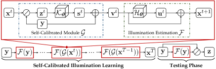
Figure 2: The entire framework of SCI. In the training phase, our SCI is composed of the illumination estimation and self-calibrated module. The self-calibrated module map is added to the original low-light input as the input of the illumination estimation at the next stage. Note that these two modules are respectively shared parameters in the whole training procedure. In the testing phase, we just utilize a single illumination estimation module.

2.2 Self-Calibrated Module

Here, we aim at defining a module to make results of each stage convergent to the same one state. We know that the input of each stage stems from the previous stage and the input of the first stage is definitely defined as the low-light observation. An intuitive idea is that whether we can bridge the input of each stage (except the first stage) and the low-light observation (i.e., the input of the first stage) to indirectly explore the convergence behavior between each stage. To this end, we introduce a self-calibrated map $\mathbf{s}$ and add it to the low-light observation to present the difference between the input in each stage and the first stage. Specifically, the self-calibrated module can be presented as

$${\mathcal{G}}(\mathbf{x}^{t}):\left\{\begin{aligned} &\mathbf{z}^{t}=\mathbf{y}\oslash\mathbf{x}^{t},\\ &\mathbf{s}^{t}=\mathcal{K}_{\bm{\vartheta}}(\mathbf{z}^{t}),\\ &\mathbf{v}^{t}=\mathbf{y}+\mathbf{s}^{t},\\ \end{aligned}\right.$$ (2)

where $t\geq 1$, $\mathbf{v}^{t}$ is the converted input for each stage, and $\mathcal{K}_{\bm{\vartheta}}$ is the introduced parameterized operator with the learnable parameters $\bm{\vartheta}$. Then the conversion for the basic unit in $t$-th stage ($t\geq 1$) can be written as

$$\mathcal{F}(\mathbf{x}^{t})\rightarrow\mathcal{F}(\mathcal{G}(\mathbf{x}^{t})).$$ (3)

Actually, our constructed self-calibrated module gradually corrects the input of each stage by integrating the physical principle to indirectly influence the output of each stage. To evaluate the effects of the self-calibrated module on the convergence, we plot tSNE distributions among results of each stage in Fig. 3, and we can easily observe that the results of each stage indeed converge to the same value. But this phenomenon cannot be found in the case without the self-calibrated module. Additionally, the above conclusion also reflects that we indeed accomplish the intention as described in the last paragraph of Sec. 2.1, i.e., training multiple cascaded blocks with the weight sharing pattern but only using the single block for testing.

We also provide the overall flowchart in Fig. 2 for understanding our established SCI framework.

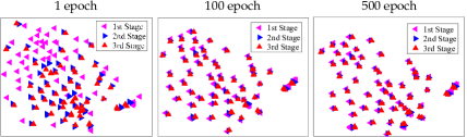
(a) w/o self-calibrated module

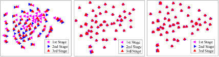
(b) w/ self-calibrated module

Figure 3: Comparing t-SNE [21] distributions in terms of the results of each stage on whether using self-calibrated module. It exhibits why we can use a single stage for testing, that is, the results of each stage in SCI can rapidly converge to the same value, but w/o self-calibrated module cannot realize it all the time.

2.3 Unsupervised Training Loss

Considering the inaccuracy of existing paired data, we adopt the unsupervised learning to enlarge the network capability. We define the total loss as $\mathcal{L}_{total}=\alpha\mathcal{L}_{f}+\beta\mathcal{L}_{s}$, where $\mathcal{L}_{f}$ and $\mathcal{L}_{s}$ represent the fidelity and smoothing loss, respectively. $\alpha$ and $\beta$ are two positive balancing parameters. The fidelity loss is to guarantee the pixel-level consistency between the estimated illumination and the input of each stage, formulated as

$$\mathcal{L}_{f}=\sum_{t=1}^{T}\|\mathbf{x}^{t}-(\mathbf{y}+\mathbf{s}^{t-1})\|^{2},$$ (4)

where $T$ is the total stage number. Actually, this function utilizes the redefined input $\mathbf{y}+\mathbf{s}^{t-1}$ to constrain the output illumination $\mathbf{x}^{t}$, rather than the hand-crafted ground truth or the plain low-light input.

The smoothness property of the illumination is a broad consensus in this task [34, 7]. Here we adopt a smoothness term with spatially-variant $\ell_{1}$ norm [4], presented as

$$\mathcal{L}_{s}=\sum_{i=1}^{N}\sum_{j\in\mathcal{N}(i)}w_{i,j}|\mathbf{x}^{t}_{i}-\mathbf{x}^{t}_{j}|,$$ (5)

where $N$ is the total number of pixels. $i$ is the $i$-th pixel. $\mathcal{N}(i)$ denotes the adjacent pixels of $i$ in its $5\times 5$ window. $w_{i,j}$ represents the weight, whose formulated form is $w_{i,j}=\exp\Big{(}-\frac{\sum_{c}((\mathbf{y}_{i,c}+\mathbf{s}_{i,c}^{t-1})-(\mathbf{y}_{j,c}+\mathbf{s}_{j,c}^{t-1}))^{2}}{2\sigma^{2}}\Big{)}$, where $c$ denotes image channel in the YUV color space. $\sigma=0.1$ is the standard deviations for the Gaussian kernels.

Setting for $\mathcal{H}_{\bm{\theta}}$		Quality		Efficiency
Blocks	Channels	PSNR	NIQE	FLOPs (G)	TIME (S)
1	3-3	20.6074	4.0091	0.0202	0.0015
2	3-3-3	20.5809	4.0075	0.0410	0.0016
3	3-3-3-3	20.4459	3.9630	0.0619	0.0017
3	3-8-8-3	20.5776	3.9711	0.2503	0.0018
3	3-16-16-3	20.5215	4.0031	0.7764	0.0022

Table 1: Quantitative comparison among different settings for $\mathcal{H}_{\bm{\theta}}$ on MIT testing dataset. In which, the basic block contains a convolutional layer with the size of $3\times 3$ and a ReLU layer. “Blocks” and “Channels” represent the numbers of the basic block and the variation of channels in the basic block, respectively.

Input	1 block(3-3)	2 blocks (3-3-3)
3 blocks (3-3-3-3)	3 blocks (3-8-8-3)	3 blocks (3-16-16-3)

Figure 4: Visual comparison among different cases in Table 1.

2.4 Discussion

In essence, the self-calibrated module plays an auxiliary role in learning a better basic block (the illumination estimation block in this work) that is cascaded to generate the overall illumination learning process with the weight sharing mechanism. More importantly, the self-calibrated module confers the convergence between results of each stage, it yet has not been explored in existing works. Moreover, the core idea of SCI is actually introducing the additional network module to assist in training, but not in the testing. It improves model characterization to realize that only using the single block for testing. That is to say, the mechanism “weight sharing + task-related self-calibrated module” may be transferred to handle other tasks for acceleration.

3 Exploring Algorithmic Properties

In this section, we perform explorations about our proposed SCI to deeply analyze its properties.

Model	PSNR	EME	NIQE	FLOPs (G)	TIME (S)
RUAS (3)	14.4372	23.5139	4.1684	0.2813	0.0063
RUAS (1) + SCI	14.7352	24.4884	3.8588	0.0936	0.0022

Table 2: SCI can be applied to improve the performance for existing works, e.g., RUAS [14]. In which RUAS (d) represents adopting d iterative blocks for the unrolling process appeared in RUAS. Here we adopt the LSRW [9] dataset for testing.

Input	RUAS (3)	RUAS (1) + SCI

Figure 5: Visual comparison among different cases in Table 2.

Dataset	Metrics	Recent Traditional Methods			Supervised Learning Methods				Unsupervised Learning Methods
		LECARM	SDD	STAR	RetinexNet	FIDE	DRBN	KinD	EnGAN	SSIENet	ZeroDCE	RUAS	Ours
MIT	PSNR$\uparrow$	17.5993	19.5241	17.6464	13.7444	17.1902	17.5910	17.0935	16.7682	10.1396	16.6114	18.5372	20.4459
	SSIM$\uparrow$	0.8556	0.8690	0.7793	0.7394	0.7853	0.7840	0.8307	0.8346	0.6456	0.8144	0.8642	0.8934
	DE$\uparrow$	6.8069	6.8253	6.3677	6.2850	6.6543	6.5914	6.7233	7.0382	6.3879	6.2116	6.9068	7.0429
	EME$\uparrow$	8.8779	8.6987	5.9128	9.1800	8.4146	7.4620	8.5482	7.9499	5.3423	7.8658	10.6396	10.9627
	LOE$\downarrow$	613.2689	505.2951	70.5651	1812.853	264.4661	705.2620	500.6578	812.9041	646.9047	508.2960	579.0181	273.3409
	NIQE$\downarrow$	4.3627	4.6477	4.2611	4.5289	5.2720	4.8166	4.2658	3.9997	5.2792	4.0933	4.1754	3.9630
LSRW	PSNR$\uparrow$	15.4747	14.6694	14.6080	15.9062	17.6694	16.1497	16.4717	16.3106	16.7380	15.8337	14.4372	15.0168
	SSIM$\uparrow$	0.4635	0.5061	0.5039	0.3725	0.5485	0.5422	0.4929	0.4697	0.4873	0.4664	0.4276	0.4846
	DE$\uparrow$	5.9980	6.7307	6.4943	6.9392	6.8745	7.2051	7.0368	6.6692	7.0988	6.8729	5.6056	6.5524
	EME$\uparrow$	24.4089	8.5431	9.4636	14.6119	5.6885	9.9968	12.0881	22.2345	9.3801	20.8010	23.5139	24.9625
	LOE$\downarrow$	34.1438	296.0794	103.2322	591.2793	194.7405	755.1283	379.8994	248.1947	261.2802	219.1284	357.4125	280.8935
	NIQE$\downarrow$	3.8189	5.6401	3.7537	4.1479	4.3277	4.5500	3.6636	3.7754	4.0631	3.7183	4.1687	3.6590

Table 3: Quantitative results in terms of two full-reference metrics including PSNR and SSIM, and four no-reference metrics including DE, EME, LOE, and NIQE on the MIT and LSRW datasets.

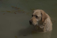
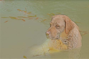
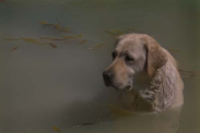
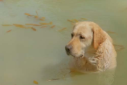
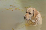
Input	RetinexNet	FIDE	DRBN	KinD
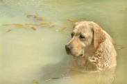
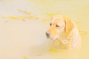
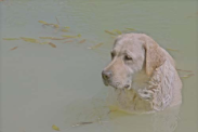
EnGAN	SSIENet	ZeroDCE	RUAS	Ours

Figure 6: Visual comparison on the MIT dataset among state-of-the-art low-light image enhancement approaches.

Input	RetinexNet	FIDE	DRBN	KinD
EnGAN	SSIENet	ZeroDCE	RUAS	Ours

Figure 7: Visual comparison on the LSRW dataset among state-of-the-art low-light image enhancement approaches.

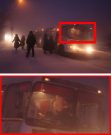
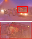
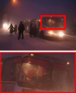
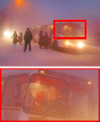
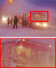
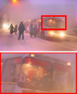
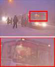
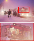
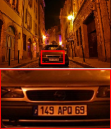
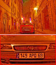
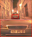
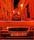
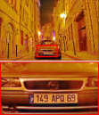
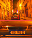
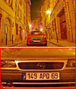
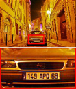
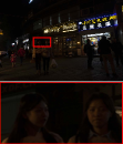
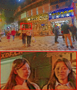
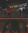
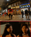
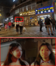
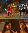
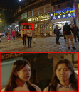
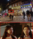
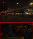
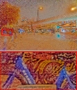
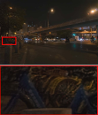
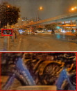
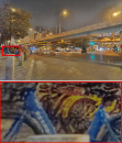
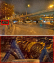
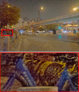
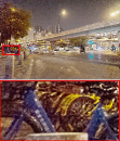
Input	RetinexNet	FIDE	DRBN	KinD	EnGAN	ZeroDCE	Ours

Figure 8: Visual comparison on some in-the-wild challenging examples. More results can be found in the Supplemental Materials.

3.1 Operation-Insensitive Adaptability

In general, the operations used in network-based methods should be fixed and cannot be changed arbitrarily since these operations are acquired under the support of massive experiments. Fortunately, our proposed algorithm emerges the surprising adaptability on different exceedingly simple, even naive settings for $\mathcal{H}_{\bm{\theta}}$. As shown in Table 1, we can easily observe that our method acquired a stable performance among different settings (numbers of the block $3\times 3$ convolution+ReLU). Further, we provide the visual comparison in Fig. 4, it can be easily observed that our SCIs with different settings all brighten the low-light observation, showing very similar enhanced results. Revisiting our designed framework, this property can be acquired lies in SCI not only converts the consensus for illumination (i.e., residual learning) but also integrates the physical principle (i.e., element-wise division operation). This experiment also verifies the effectiveness and correctness of our designed SCI.

Method		SIZE (M)	FLOPs (G)	TIME (S)
Supervised	RetinexNet	0.8383	136.0151	0.1192
	FIDE	8.6213	57.2401	0.5936
	DRBN	0.5770	37.7902	0.0533
	KinD	8.5402	29.1303	0.1814
Unsupervised	EnGAN	8.6360	61.0102	0.0097
	SSIENet	0.6824	34.6070	0.0272
	ZeroDCE	0.0789	5.2112	0.0042
	RUAS	0.0014	0.2813	0.0063
	Ours	0.0003	0.0619	0.0017

Table 4: The model size, FLOPs and running time (GPU-seconds for inference) of CNN-based methods and our SCI.

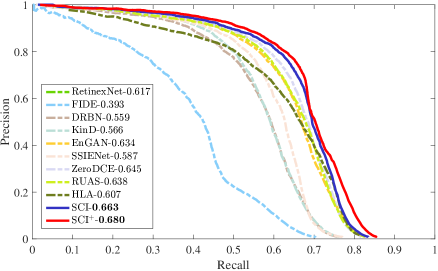
Figure 9: Precision-Recall curve on the DARK FACE dataset. All compared methods and SCI fine-tune the detector on the enhanced results. SCI⁺ is to jointly train the detector and SCI over the combination of losses for detection and enhancement.

3.2 Model-Irrelevant Generality

Our SCI is actually a generalized learning paradigm if not limiting the task-related self-calibrated module, so ideally, it can be directly applied to existing works. Here, we take the recently-proposed representative work RUAS [14] as an example to make an exploration. Table 2 and Fig. 5 demonstrate the quantitative and qualitative comparison before/after using our SCI to train RUAS. Obviously, although we just utilized a single block (i.e., RUAS (1)) used in the unrolling process of RUAS to evaluate our training process, the performance still attains significant improvement. More importantly, our method can remarkably suppress the overexposure that appeared in the original RUAS. This experiment reflects our learning framework is indeed flexible enough and has a strong model-irrelevant generality. Moreover, it indicates that perhaps our method can be transferred to arbitrary illumination-based low-light image enhancement works and we will try doing it in the future.

4 Experimental Results

In this section, we first provided all implementation details. Then we made experimental evaluations. Next, we applied enhancement methods to dark face detection and nighttime semantic segmentation. Finally, we conducted algorithmic analyses for SCI. All the experiments were performed on a PC with a single TITAN X GPU.

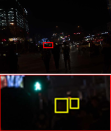
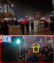
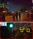
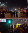
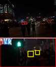
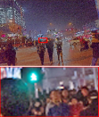
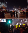
Input	KinD	EnGAN	ZeroDCE	RUAS	HLA	SCI	SCI+

Figure 10: Visual comparison of face detection on the DarkFace dataset. More results can be found in the Supplemental Materials.

Input	DRBN	KinD	EnGAN	ZeroDCE	RUAS	SCI	GT

Figure 11: Visual results of semantic segmentation on the ACDC dataset. More results can be found in the Supplemental Materials.

Method	RO	SI	BU	WA	FE	PO	TL	TS	VE	TE	SK	PE	RI	CA	TR	MO	BI	mIoU
RetinexNet	90.6	67.2	74.3	35.5	37.4	41.0	36.4	31.9	67.3	13.0	79.4	30.7	4.1	0.3	65.3	5.9	37.1	42.1
FIDE	90.4	68.8	77.0	40.1	35.4	42.0	42.1	42.4	68.0	16.4	81.4	39.6	8.7	2.4	55.0	11.0	40.8	44.8
DRBN	91.8	69.0	76.9	39.5	38.3	43.3	41.8	43.9	68.1	16.5	80.1	36.6	7.6	1.7	64.2	12.1	44.2	45.6
KinD	89.5	66.7	75.3	35.6	37.5	43.1	46.3	38.9	68.4	16.1	81.3	40.4	10.5	0.8	48.9	3.9	43.9	44.5
EnGAN	89.7	67.8	76.8	39.0	38.8	43.1	40.8	42.2	68.8	18.4	81.2	39.4	8.0	0.3	46.0	9.7	46.1	44.5
SSIENet	89.0	65.4	76.4	36.7	38.6	40.9	41.8	40.5	69.2	20.2	81.6	34.6	8.0	1.3	46.5	10.4	39.9	43.6
ZeroDCE	90.1	67.2	77.3	40.2	37.8	41.9	42.2	41.9	69.1	22.3	81.9	36.3	7.0	0.3	54.3	11.8	47.3	45.2
RUAS	90.4	66.7	76.2	37.6	38.8	42.9	39.6	40.9	69.0	18.6	81.5	39.6	9.5	0.6	49.6	13.5	46.6	44.8
Ours	92.1	70.0	78.3	39.3	39.8	43.0	46.6	44.2	69.9	19.7	81.8	38.7	6.5	0.7	64.9	9.0	42.4	46.3

Table 5: Quantitative results of nighttime semantic segmentation on the ACDC dataset. The symbol set {RO, SI, BU, WA, FE, PO, TL, TS, VE, TE, SK, PE, RI, CA, TR, MO, BI} represents {road, sidewalk, building, wall, fence, pole, traffic light, traffic sign, vegetation, terrain, sky, person, rider, car, train, motorcycle, bicycle}. Notice that we retrained the segmentation model on the enhanced results that were generated by all the compared methods. The best result is in red whereas the second best one is in blue.

4.1 Implementation Details

Parameter Settings. In the training process, we used the ADAM optimizer [12] with parameters $\beta_{1}=0.9$, $\beta_{2}=0.999$, and $\epsilon=10^{-8}$. The minibatch size was set to 8. The learning rate was initialized to $10^{-4}$. The training epoch number was set to 1000. We adopt 3 convolution + ReLU with 3 channels as our default setting for $\mathcal{H}_{\bm{\theta}}$ in our all experiments according to conclusion in Sec. 3.1. Self-calibrated module contains four convolution layers, which ensures the lightweight of the training process. In fact, the form of the network may not be fixed, and we have done experiments to verify it in the Supplementary Materials.

Compared Methods. As for low-light image enhancement, we compared our SCI with four recently-proposed model-based methods (including LECARM [17], SDD [10], STAR [26]), four advanced supervised learning methods (including RetinexNet [3], KinD [34], FIDE [27], DRBN [30]), and four unsupervised learning methods (including EnGAN [11], SSIENet [33], ZeroDCE [7], and RUAS [14]). As for dark face detection, except for performing the above-mentioned network-based enhancement works before the detector, we also compared the recently-proposed dark face detection method HLA [24].

Benchmarks Description and Metrics. As for low-light image enhancement, we randomly sampled 100 images from MIT dataset [2] and 50 testing image from LSRW dataset [9] for testing. We used two full-reference metrics including PSNR and SSIM, five no-reference metrics including DE [20], EME [1], LOE [23] and NIQE [23]. As for dark face detection, we utilized the DARK FACE dataset [31] that consisted of 1000 challenging testing images that randomly sampled from the sub-challenge of UG2+ PRIZE CHALLENGE held at CVPR 2021. We considered the detection accuracy precision and recall rate as the evaluated metric. As for nighttime semantic segmentation, we utilized 400 images in ACDC [19] for training and the remaining 106 images as the evaluated dataset. The evaluated metrics were defined as IoU and mIoU.

4.2 Experimental Evaluation on Benchmarks

Performance Evaluation. As shown in Table 3, our SCI achieved competitive performance, especially in no-reference metrics. As shown in Fig. 6-7, advanced deep networks generated the unknown veils, leading to the inconspicuous details and unnatural colors. By comparison, our SCI achieved the best visual quality with vivid colors and prominent textures. More visual comparisons can be found in the Supplemental Materials.

Computational Efficiency. Further, we reported the model size, FLOPs, and running time (GPU-seconds) of some recently-proposed CNN-based methods in Table 4. Obviously, our proposed SCI is the most lightweight compared with other networks, and significantly superior to others.

4.3 In-the-Wild Experimental Evaluation

Low-light image enhancement in the wild scenarios is extremely challenging. The control of the partial overexposure information of the image, the correction of the overall color, and the preservation of image details are all problems that need to be solved urgently. Here, we tested lots of challenging in-the-wild examples from the DARK FACE [31] and ExDark [15] datasets. As demonstrated in Fig. 8, through a large number of experiments, it can be seen that our method achieved more satisfactory visualization results than others, especially in the exposure level, structure depict, color presentation. Limited to the space, we provided more comparisons in the Supplemental Materials.

4.4 Dark Face Detection

We utilized the S3FD [32], a well-known face detection algorithm to evaluate the dark face detection performance. Note that the S3FD was trained with the WIDER FACE dataset [29] as presented in the original S3FD, and we used the pre-trained model of S3FD to fine-tune the images enhanced by various methods.

At the same time, we performed a new method named SCI⁺ which embed our SCI as a basic module into the front of S3FD for joint training over the combination of losses for task and enhancement. As reported in Fig. 9, our methods (SCI and SCI⁺) realized the best scores among all compared method, and the reinforced version acquired the better performance than the fine-tune version. Fig. 10 further demonstrated the visual comparison. It can be easily observed that with applying our SCI, the smaller objects can also be detected, while other methods failed to do so, as shown in the zoomed-in regions.

4.5 Nighttime Semantic Segmentation

Here we adopted the PSPNet [35] as the baseline to evaluate the segmentation performance on the pattern “pre-train + fine-tune” (similar to the version of SCI in dark face detection) for all methods. Table 5 and Fig. 11 demonstrated the results of quantitative and qualitative comparison among different methods. Our performance is significantly superior to other state-of-the-art methods. As shown in the zoomed-in regions in Fig. 11, all compared methods produced some unknown artifacts to damage the quality of the generated segmentation map.

RetinexNet	KinD	SSIENet	Ours

Figure 12: Comparing the decomposed components among different illumination-based networks. Zoom in for best view.

4.6 Algorithmic Analyses

Comparing Decomposed Components. Actually, our SCI belongs to illumination-based learning methods, the enhanced visual quality heavily depends on the estimated illumination. Here we compared our SCI with three representative illumination-based learning approaches, including RetinexNet, KinD, and SSIENet. As demonstrated in Fig. 12, we can easily see that our estimated illumination kept an excellent smoothness property. It ensured our generated reflectance more visually friendly.

Input	w/o residual	w/ residual	Ours

Figure 13: Analyze different modes in the illumination learning.

Ablation Study. We compared the performance of different modes in Fig. 13. Learning the illumination directly will cause the image to be overexposed. The process of learning residuals between the illumination and the input indeed suppressed the overexposure, but the overall image quality is still not high, especially for the grasp of details. By comparison, the enhanced results using our method not only suppress the overexposure but also enrich image structures.

5 Concluding Remarks

In this paper, we successfully established a lightweight yet effective framework, Self-Calibrated Illumination (SCI) for low-light image enhancement toward different real-world scenarios. We not only made a thorough exploration to take on the excellent properties of SCI, but also we performed extensive experiments to indicate our effectiveness and superiority in low-light image enhancement, dark face detection, and nighttime semantic segmentation.

Broader Impacts. From the task’s perspective, SCI provides an efficient and effective learning framework and has received extremely superior performance in both image quality and inference speed. Maybe it will be a brace to enter a new high-speed and high-quality era for low-light image enhancement. As for the method design, SCI opens a new perspective (i.e., introducing the auxiliary process for boosting the model capability of the basic unit in the training phase) to improve the practicability toward real-world scenarios for other low-level vision problems.

Acknowledgements: This work is supported by the National Key R&D Program of China (2020YFB1313503), the National Natural Science Foundation of China (Nos. 61922019, 61733002 and 62027826), and the Fundamental Research Funds for the Central Universities.

References

- [1] Sos S Agaian, Blair Silver, and Karen A Panetta. Transform coefficient histogram-based image enhancement algorithms using contrast entropy. IEEE Transactions on Image Processing, 16(3):741–758, 2007.
- [2] Vladimir Bychkovsky, Sylvain Paris, Eric Chan, and Frédo Durand. Learning photographic global tonal adjustment with a database of input/output image pairs. In Proceeding of the IEEE Conference on Computer Vision and Pattern Recognition, pages 97–104, 2011.
- [3] Wei Chen, Wenjing Wang, Wenhan Yang, and Jiaying Liu. Deep retinex decomposition for low-light enhancement. In British Machine Vision Conference, pages 1–12, 2018.
- [4] Qingnan Fan, Jiaolong Yang, David Wipf, Baoquan Chen, and Xin Tong. Image smoothing via unsupervised learning. ACM Transactions on Graphics), 37(6):1–14, 2018.
- [5] Xueyang Fu, Yinghao Liao, Delu Zeng, Yue Huang, Xiao-Ping Zhang, and Xinghao Ding. A probabilistic method for image enhancement with simultaneous illumination and reflectance estimation. IEEE Transactions on Image Processing, 24(12):4965–4977, 2015.
- [6] Xueyang Fu, Delu Zeng, Yue Huang, Xiao-Ping Zhang, and Xinghao Ding. A weighted variational model for simultaneous reflectance and illumination estimation. In Proceeding of the IEEE Conference on Computer Vision and Pattern Recognition, pages 2782–2790, 2016.
- [7] Chunle Guo, Chongyi Li, Jichang Guo, Chen Change Loy, Junhui Hou, Sam Kwong, and Runmin Cong. Zero-reference deep curve estimation for low-light image enhancement. IEEE Transactions on Pattern Analysis and Machine Intelligence, 2021.
- [8] Xiaojie Guo, Yu Li, and Haibin Ling. Lime: Low-light image enhancement via illumination map estimation. IEEE Transactions on Image Processing, 26(2):982–993, 2017.
- [9] Jiang Hai, Zhu Xuan, Ren Yang, Yutong Hao, Fengzhu Zou, Fang Lin, and Songchen Han. R2rnet: Low-light image enhancement via real-low to real-normal network. arXiv preprint arXiv:2106.14501, 2021.
- [10] Shijie Hao, Xu Han, Yanrong Guo, Xin Xu, and Meng Wang. Low-light image enhancement with semi-decoupled decomposition. IEEE Transaction on Multimedia, 2020.
- [11] Yifan Jiang, Xinyu Gong, Ding Liu, Yu Cheng, Chen Fang, Xiaohui Shen, Jianchao Yang, Pan Zhou, and Zhangyang Wang. Enlightengan: Deep light enhancement without paired supervision. IEEE Transactions on Image Processing, 30:2340–2349, 2021.
- [12] Diederik P Kingma and Jimmy Ba. Adam: A method for stochastic optimization. In International Conference on Learning Representations, pages 1–13, 2014.
- [13] Mading Li, Jiaying Liu, Wenhan Yang, Xiaoyan Sun, and Zongming Guo. Structure-revealing low-light image enhancement via robust retinex model. IEEE Transactions on Image Processing, 27(6):2828–2841, 2018.
- [14] Risheng Liu, Long Ma, Jiaao Zhang, Xin Fan, and Zhongxuan Luo. Retinex-inspired unrolling with cooperative prior architecture search for low-light image enhancement. In Proceedings of the IEEE Conference on Computer Vision and Pattern Recognition, pages 10561–10570, 2021.
- [15] Yuen Peng Loh and Chee Seng Chan. Getting to know low-light images with the exclusively dark dataset. Computer Vision and Image Understanding, 178:30–42, 2019.
- [16] Zia-ur Rahman, Daniel J Jobson, and Glenn A Woodell. Retinex processing for automatic image enhancement. JEI, 13(1):100–111, 2004.
- [17] Yurui Ren, Zhenqiang Ying, Thomas H Li, and Ge Li. Lecarm: Low-light image enhancement using the camera response model. IEEE Transactions on Circuits and Systems for Video Technology, 29(4):968–981, 2018.
- [18] Christos Sakaridis, Dengxin Dai, and Luc Van Gool. Guided curriculum model adaptation and uncertainty-aware evaluation for semantic nighttime image segmentation. In Proceedings of the IEEE/CVF International Conference on Computer Vision, pages 7374–7383, 2019.
- [19] Christos Sakaridis, Dengxin Dai, and Luc Van Gool. Acdc: The adverse conditions dataset with correspondences for semantic driving scene understanding. arXiv preprint arXiv:2104.13395, 2021.
- [20] Claude E Shannon. A mathematical theory of communication. The Bell system technical journal, 27(3):379–423, 1948.
- [21] Laurens Van der Maaten and Geoffrey Hinton. Visualizing data using t-sne. Journal of machine learning research, 9(11), 2008.
- [22] Ruixing Wang, Qing Zhang, Chi-Wing Fu, Xiaoyong Shen, Wei-Shi Zheng, and Jiaya Jia. Underexposed photo enhancement using deep illumination estimation. In Proceeding of the IEEE Conference on Computer Vision and Pattern Recognition, pages 6849–6857, 2019.
- [23] Shuhang Wang, Jin Zheng, Hai-Miao Hu, and Bo Li. Naturalness preserved enhancement algorithm for non-uniform illumination images. IEEE Transactions on Image Processing, 22(9):3538–3548, 2013.
- [24] Wenjing Wang, Wenhan Yang, and Jiaying Liu. Hla-face: Joint high-low adaptation for low light face detection. In Proceedings of the IEEE Conference on Computer Vision and Pattern Recognition, 2021.
- [25] Xinyi Wu, Zhenyao Wu, Hao Guo, Lili Ju, and Song Wang. Dannet: A one-stage domain adaptation network for unsupervised nighttime semantic segmentation. In Proceedings of the IEEE/CVF Conference on Computer Vision and Pattern Recognition, pages 15769–15778, 2021.
- [26] Jun Xu, Yingkun Hou, Dongwei Ren, Li Liu, Fan Zhu, Mengyang Yu, Haoqian Wang, and Ling Shao. Star: A structure and texture aware retinex model. IEEE Transactions on Image Processing, 29:5022–5037, 2020.
- [27] Ke Xu, Xin Yang, Baocai Yin, and Rynson WH Lau. Learning to restore low-light images via decomposition-and-enhancement. In Proceeding of the IEEE Conference on Computer Vision and Pattern Recognition, pages 2281–2290, 2020.
- [28] Li Xu, Qiong Yan, Yang Xia, and Jiaya Jia. Structure extraction from texture via relative total variation. ACM Transactions on Graphics, 2012.
- [29] Shuo Yang, Ping Luo, Chen Change Loy, and Xiaoou Tang. Wider face: A face detection benchmark. In Proceeding of the IEEE Conference on Computer Vision and Pattern Recognition, 2016.
- [30] Wenhan Yang, Shiqi Wang, Yuming Fang, Yue Wang, and Jiaying Liu. From fidelity to perceptual quality: A semi-supervised approach for low-light image enhancement. In Proceeding of the IEEE Conference on Computer Vision and Pattern Recognition, pages 3063–3072, 2020.
- [31] Wenhan Yang, Ye Yuan, Wenqi Ren, Jiaying Liu, Walter J Scheirer, Zhangyang Wang, Taiheng Zhang, Qiaoyong Zhong, Di Xie, Shiliang Pu, et al. Advancing image understanding in poor visibility environments: A collective benchmark study. IEEE Transactions on Image Processing, 29:5737–5752, 2020.
- [32] Shifeng Zhang, Xiangyu Zhu, Zhen Lei, Hailin Shi, Xiaobo Wang, and Stan Z Li. S3fd: Single shot scale-invariant face detector. In Proceedings of the IEEE international conference on computer vision, pages 192–201, 2017.
- [33] Yu Zhang, Xiaoguang Di, Bin Zhang, and Chunhui Wang. Self-supervised image enhancement network: Training with low light images only. arXiv, pages arXiv–2002, 2020.
- [34] Yonghua Zhang, Xiaojie Guo, Jiayi Ma, Wei Liu, and Jiawan Zhang. Beyond brightening low-light images. International Journal of Computer Vision, pages 1–25, 2021.
- [35] Hengshuang Zhao, Jianping Shi, Xiaojuan Qi, Xiaogang Wang, and Jiaya Jia. Pyramid scene parsing network. In Proceedings of the IEEE conference on computer vision and pattern recognition, pages 2881–2890, 2017.