Superconducting microwave resonators with non-centrosymmetric nonlinearity

Abstract

We investigated both theoretically and experimentally open-ended coplanar waveguide resonators with rf SQUIDs embedded in the central conductor at different positions. These rf SQUIDs can be tuned by an external magnetic field and thus may exhibit the non-centrosymmetric nonlinearity of $\chi^{(2)}$ type with suppressed Kerr nonlinearity. We demonstrated that this nonlinearity allows for efficient mixing of $\lambda/2$ and $\lambda$ modes in the cavity and thus enables various parametric effects with three wave mixing. These effects are the second harmonic generation, the half tone generation, the parametric amplification in both degenerate and non-degenerate regimes and deamplification in degenerate regime.

I Introduction

Superconducting coplanar waveguide (CPW) resonators with embedded Josephson junctions and SQUIDs are widely used for parametric amplification Castellanos-Beltran2007 ; Yamamoto2008 ; Eichler2011 , bifurcation-based quantum detection Manucharyan2007 ; Metcalfe2007 ; Vijay2009 ; Tancredi2013 ; Wustmann2013 , generation of nonclassical states of microwaves Castellanos-Beltran2008 ; Wustmann2013 ; Zhong2013 ; Schneider2018 , studying the dynamical Casimir effect and photon field correlations Wilson2011 ; Lahteenmaki2013 , parametric down conversion Chang2020 , etc. At the working microwave frequencies (up to approximately 20 GHz), superconducting resonators have very low losses, while the Josephson tunnel junctions facilitate the parametric effects. The operation of these circuits is usually based either on the Kerr nonlinearity of the Josephson inductance Castellanos-Beltran2007 ; Metcalfe2007 ; Vijay2009 ; Tancredi2013 ; Castellanos-Beltran2008 ; Palacios-Laloy2008 ; Bourassa2012 ; Wustmann2013 ; Eichler2014 or on a periodic modulation of the dc SQUID inductance by means of an alternating magnetic flux Yamamoto2008 ; Schneider2018 ; Wilson2011 ; Lahteenmaki2013 .

Recently, the toolbox of superconducting quantum technologies Devoret2013 has been supplemented with the elements having non-centrosymmetric nonlinearity of $\chi^{(2)}$ type Shen1984 . These superconducting elements are based either on rf SQUIDs Yurke1989 ; Zorin2016 ; Zorin2017 , asymmetric dc SQUIDs Chang2020 , or the multijunction SQUID, i.e., the so-called superconducting nonlinear asymmetric inductive elements (SNAILs) Zorin2017 ; Frattini2017 . For the optimal constant flux $\Phi_{e}$ applied to the SQUID loop, the current-phase relation in these elements may have the Kerr-free shape Zorin2016 ; Zorin2017 ; Frattini2017 ,

$$I(\varphi)\approx(\varphi-\beta\varphi^{2})\varphi_{0}L^{-1}_{s},$$ (1)

where $\varphi_{0}=\Phi_{0}/2\pi$ is the reduced magnetic flux quantum, $L_{s}$ is the linear SQUID inductance, and nonlinear coefficient $\beta$ is the electrical analog of susceptibility tensor $\chi^{(2)}$ in optics Shen1984 . The nonlinear relation (1) enables three wave mixing (3WM) including frequency doubling and parametric down-conversion. Optical crystals having nonzero susceptibility $\chi^{(2)}$ are quite rare in nature Kurtz1968 and fabrication of optical fibers with non-centrosymmetric nonlinearity suitable for engineering traveling wave amplifiers is not as easy as fabrication of the silica fibers with Kerr nonlinearity Agrawal . However, the superconducting technology allows the fabrication of the transmission lines with embedded rf SQUIDs. These circuits can have a nonlinearity given by Eq.(1) and, thus, enable parametric amplification of traveling microwaves using 3WM Zorin2016 ; Zorin2017 ; Miano2018 . A recent study of the effect of parameter variations Peatain2021 confirmed that such a parametric amplifier is a strong candidate for achieving a high gain in a wide frequency band together with a high fabrication yield.

Parametric amplification based on serial arrays of SNAILs inserted in the CPW resonators was recently demonstrated by the Yale group. These Josephson parametric amplifiers with 3WM clearly demonstrated a number of advantages of the Kerr-free operation including an improved dynamic range Sivak2019 , relatively large saturation power with a widely tunable bandwidth Frattini2018 ; Miano2021 , and near-quantum-limited performance Sivak2020 .

In this paper we first examined Nb open-ended CPW resonators with rf SQUIDs embedded in their center, i.e. in the antinode of the fundamental ($\lambda/2$) mode. The parameters of rf SQUIDs were close to those of the rf SQUIDs exploited in the Josephson traveling wave parametric amplifiers (JTWPA) with 3WM Zorin2017 . Our primary motivation was the investigation of these tunable nonlinear elements, including the determination of their electric parameters. These parameters were found from the dependence of the resonant frequency on magnetic flux $\Phi_{e}$.

The tunability of the rf SQUID inductance has been utilized earlier in microwave circuits for the coupling of, for example, two resonators Wulschner2016 or a resonator and a phase qubit Allman2014 . Here we investigate the circuit with the intermode coupling based on the nonlinear characteristic of the rf SQUID given by Eq. (1). For this purpose we designed CPW resonators with the rf SQUID positioned at one third of the open-ended resonator length. Thus, we engineered an artificial medium with a nonlinearity of $\chi^{(2)}$ type enabling efficient coupling of primarily the $\lambda/2$ and $\lambda$ modes. In this circuit, we demonstrated a number of parametric 3WM phenomena including the second harmonic generation (SHG), the half tone generation (HTG), the parametric amplification in both degenerate and non-degenerate regimes, etc. The improved design of a circuit with a high degree of intermode coupling is proposed.

II Design and fabrication

The design of our open-ended superconducting CPW resonators (the microwave analog of a Fabry-Perot cavity) with an embedded rf SQUID is schematically shown in Fig. 1. The resonant frequencies of $\lambda/2$ mode were designed to be around 3.9 GHz. The resonator length was 16.136 mm with a center-conductor width of $w=32~{}\mu$m and gaps between this conductor and the ground plane conductors of $s=16~{}\mu$m. The nominal thickness of Nb layer was 200 nm. These dimensions of the CPW waveguide yielded a wave impedance of $Z_{0}=50~{}\Omega$. This impedance was matched with the impedance of the input and output lines. The CPW waveguide parameters were chosen similar to those of the CPW transmission line used in the design of the JTWPAs Zorin2017 . The total inductance and the total capacitance of the resonator were $L_{\textrm{tot}}=\ell d=6.454$ nH and $C_{\textrm{tot}}=cd=2.582$ pF, respectively. The corresponding specific values were $\ell=0.4$ pH/$\mu$m and $c=0.16$ fF/$\mu$m.

The input, $C_{\textrm{in}}$, and output, $C_{\textrm{out}}$, capacitances of the resonator were realized either as gap capacitances with spacing $w_{g}=2~{}\mu$m or interdigital capacitances having 4 fingers (see, e.g., Ref. Goeppl2008 ). The finger width and spacing between the fingers were 2 $\mu$m, while the finger length varied from 10 $\mu$m to 50 $\mu$m. The nominal capacitance values $C_{\textrm{in}}$ and $C_{\textrm{out}}$ for Sample 1 were 1.8 fF and 2.8 fF, respectively, and 2.8 fF and 14 fF for Sample 2, respectively. In the case of Sample 1 these values result in a coupling quality factor Goeppl2008 $Q_{c}=94\,000$ for the fundamental $\lambda/2$ mode, while the loaded quality factor $Q\ll Q_{c}$. The experimental value $Q\approx 4\,000\,...\,8\,000$ was increasing for an increasing drive power $-105\,$dBm$\,...\,-90\,$dBm, what can be explained by the saturation of microscopic two-level systems Martinis2005 ; Burnett2016 and indicates that $Q$ is mainly determined by the dielectric loss in the deposited SiO₂ layer deGraaf2020 and/or in the Josephson junction barriers Weides2011 .

Sample 2 was designed to be critically coupled with $Q_{c}=5\,100$, approximately equal to the internal quality factor, which is an optimum in the compromise of coupling strength and quality factor needed for pronounced nonlinear interactions Goeppl2008 . For this sake, we created a strongly coupled output port, i.e., $C_{\textrm{out}}$ was chosen much larger than $C_{\textrm{in}}$ Wustmann2013 . The resulting experimental quality factor was $Q\approx 2\,000$ and didn’t exhibit significant temperature dependence in the range from 20 mK up to 4.2 K.

A local magnetic field was applied to the rf SQUID loops via a control-current line (the thin Nb wire seen very close to the upper ground plane in Fig.1c). The thin-film rf SQUID inductances had the meander shape with a few turns (see Fig.1c) giving the nominal values of $L_{g}$ around 30 pH.

The samples were fabricated using the Nb-trilayer technology with a critical current density $j_{c}$ from 200 A$/$cm² to 500 A$/$cm² on a Si/SiO₂ substrate Dolata2005 . The self-capacitance $C_{J}$ of the Josephson junctions with a nominal area of 1 $\mu$m² was in the range from $45-50$ fF. The details of manufacturing similar CPW resonators with embedded Josephson junctions and dc SQUIDs were described in Ref. Khabipov2014 .

III Linear regime. Characterization of the rf SQUIDs

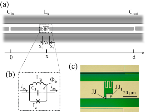
Figure 1: (a) Schematic of the open-ended coplanar transmission line of total length $d$ including inductance $L_{s}(\Phi)$ of physical length $\Delta x$ embedded at position $x$. Electrical diagram (b) and microphotograph (c) of the Nb rf SQUID, where an auxiliary (large) Josephson junction (JJ₁) in series with the primary (small) junction (JJ) was added as a stud-via.

The inverse inductance for a small alternating current $i_{\textrm{ac}}$ (see Fig. 1b) passing through the rf SQUID is given by the expression

$$L_{s}^{-1}[\Phi_{\textrm{dc}}(\Phi_{e})]=L_{g}^{-1}\left\{1+\beta_{L}\cos[\Phi_{\textrm{dc}}(\Phi_{e})/\varphi_{0}]\right\}.$$ (2)

Here we assumed that the Josephson tunnel junction in the SQUID loop has the sinusoidal (conventional) current-phase relation. The constant flux in the SQUID loop $\Phi_{\textrm{dc}}$ is found by solving the transcendental equation KK-book1986

$$\Phi_{e}=\Phi_{\textrm{dc}}+\beta_{L}\varphi_{0}\sin(\Phi_{\textrm{dc}}/\varphi_{0}),$$ (3)

where $\Phi_{e}$ is applied magnetic flux, $\beta_{L}=L_{g}I_{c}/\varphi_{0}<1$ is the dimensionless screening parameter, $L_{g}$ is the SQUID inductance, and $I_{c}$ is the Josephson critical current. Embedding the rf SQUID in the CPW resonator causes a shift of the resonant frequency. The flux dependence of the rf SQUID inductance given by Eq. (2) allows the characterization of the rf SQUID by measuring that frequency shift. This method is conceptually similar to that developed by Rifkin and Deaver, Jr. Rifkin1976 for the characterization of rf SQUIDs having inductive coupling to a rf-driven tank circuit Ilichev2001 (see also Ref. Wegner2021 ).

The resonant frequency of the $n$-th mode, $n\lambda/2=d$, $n=1,2,...$, is given by the general formula (see Eqs. (43) and (44) of Appendix):

$$\frac{\omega_{n}}{\omega_{n}^{(0)}}=1-\frac{L_{s}(\Phi_{\textrm{dc}})}{L_{\textrm{tot}}}\sin^{2}\frac{n\pi x}{d}+\frac{\Delta x}{d}.$$ (4)

For the first mode, $n=1$, and the central position of the rf SQUID, $x=d/2$, expression (4) takes the form

$$\frac{\omega_{1}}{\omega_{1}^{(0)}}\approx 1-\frac{L_{g}/L_{\textrm{tot}}}{1+\beta_{L}\cos(\Phi_{\textrm{dc}}/\varphi_{0})},$$ (5)

where we used Eq. (2) and neglected the small constant term $\Delta x/d$ $\approx\,10^{-3}$ because of the small SQUID size $\Delta x$.

The bare resonant frequency in Eq. (5) is Pozar1993

$$\omega_{n}^{(0)}=\frac{1}{\sqrt{L_{\textrm{eff},n}C_{\textrm{eff},n}}}=\frac{n\pi}{\sqrt{L_{\textrm{tot}}C_{\textrm{tot}}}},$$ (6)

where the effective $LC$ parameters for the $n$-th mode are given by the following expressions Wallquist2006 :

$$\frac{1}{L_{\textrm{eff},n}}=\frac{(k_{n}d)^{2}}{2L_{\textrm{tot}}}\left[1+\frac{\sin 2k_{n}d}{2k_{n}d}\right]=\frac{(n\pi)^{2}}{2L_{\textrm{tot}}}$$ (7)

and

$$C_{\textrm{eff},n}=\frac{C_{\textrm{tot}}}{2}\left[1+\frac{\sin 2k_{n}d}{2k_{n}d}\right]=\frac{C_{\textrm{tot}}}{2}$$ (8)

with $k_{n}=k^{(0)}_{n}=n\pi/d$. As long as the rf SQUID plasma frequency $\omega_{J}$ is sufficiently high, that is $\omega_{J}=1/\sqrt{L_{g}C_{J}}\approx 2\pi\times 120$ GHz $\gg\omega_{n}^{(0)}$, the effect of the Josephson junction self-capacitance $C_{J}$ on the resulting resonant frequency $\omega_{n}$ can safely be neglected at least for the first 10 modes.

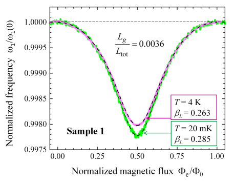
Figure 2: One period of the normalized dependence of the resonant frequency of the fundamental $\lambda/2$-mode, $\omega_{1}(\Phi_{e})/\omega_{1}(0)$, on the normalized magnetic flux, $\Phi_{e}/\Phi_{0}$, measured at two temperatures in Sample 1. The resonant frequency is normalized to its maximum value of $\omega_{1}(0)=\omega_{1}^{(0)}\{1-L_{g}/[(1+\beta_{L})L_{\textrm{tot}}]\}$. In this sample, the rf SQUID is embedded in the center of the CPW resonator, $x=0.5d$. Dashed lines denote the fitting curves using formula (5). Both measurements were performed in a dilution refrigerator.

The measurements of the resonant frequency of the fundamental mode ($n=1$) were performed (see Appendix C for details) in a dilution refrigerator at temperatures $T=20$ mK $\pm$ 0.2 mK and $T=4$ K $\pm$ 0.1 K. The resonant frequency showed a clear periodic dependence on the control current producing the magnetic flux $\Phi_{e}$. The experimental data and the fits using formula (5) are presented in Fig. 2. Because the values of the resonant frequency $\omega_{1}(0)$ found in both experiments at zero magnetic flux $\Phi_{e}$ were identical (3.917 GHz), we concluded that resonator inductance $L_{\textrm{tot}}$ doesn’t depend on temperature.

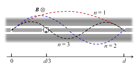
Figure 3: Geometry of the open-ended CPW resonator with rf SQUIDs embedded at $x=d/3$, yielding maximum coupling of the first two resonant modes. Dashed lines show schematically the profiles of standing waves of the current for modes $n=1$, $n=2$, and $n=3$.

The participation ratio value, $L_{g}/L_{\textrm{tot}}=0.0036$, found from fitting the experimental curves turned out to be also temperature independent. The values of the SQUID-parameter $\beta_{L}$ for different temperatures, $\beta_{L}^{(4\textrm{K})}=0.263$ and $\beta_{L}^{(20\textrm{mK})}=0.285$ (see Fig. 2), clearly pointed to a temperature dependence of the critical current. Thus, the ratio of the critical current values at the two temperatures is

$$\iota=\frac{I_{c}^{(20\textrm{mK})}}{I_{c}^{(4\textrm{K})}}=\frac{\beta_{L}^{(20\textrm{mK})}}{\beta_{L}^{(4\textrm{K})}}\approx 1.08.$$ (9)

Using the Ambegaokar-Baratoff formula AB1963 for the temperature dependence of the critical current of an ideal tunnel junction between two identical BCS superconductors with critical temperature $T_{c}=T_{c}^{\textrm{(Nb)}}\approx$ 9.0 K (here $T_{c}^{\textrm{(Nb)}}$ is the critical temperature of our Nb films) we arrive at the same value of $\iota_{\textrm{AB}}=1.08$.

IV Nonlinear effects

Setting the external magnetic flux $\Phi_{e}$ in Eq. (3) such that the constant flux $\Phi_{\textrm{dc}}=\Phi_{0}/4$, that is

$$\Phi_{e}/\varphi_{0}=\pi/2+\beta_{L},$$ (10)

yields the Kerr-free nonlinear inductance of the rf SQUID of the form given by Eq. (1) Zorin2016 . The nonlinear coefficient in the current-phase relation (1), given in the general case by

$$\beta=0.5\beta_{L}\frac{\sin(\Phi_{\textrm{dc}}/\varphi_{0})}{1+\beta_{L}\cos(\Phi_{\textrm{dc}}/\varphi_{0})},$$ (11)

then equals $\beta=0.5\beta_{L}$. For $\Phi_{\textrm{dc}}=\Phi_{0}/4$, the linear inductance of the rf SQUID (2) is equal to its geometrical inductance, $L_{s}=L_{g}$, while the inductance of the Josephson junction is infinite, $L_{J}=\varphi_{0}/[I_{c}\cos(\Phi_{\textrm{dc}}/\varphi_{0})]\rightarrow\infty$.

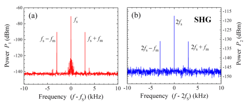
Figure 4: SHG in Sample 2 ($x=d/3$ and $\beta_{L}=0.44$). (a) Spectrum of the amplitude-modulated signal (15) with carrier frequency of $f_{s}=\omega_{s}/2\pi$ = 3.8858 GHz $\approx\omega_{1}/2\pi$ = 3.888 GHz, modulation frequency of $f_{m}=\omega_{m}/2\pi$ = 3 kHz, and modulation index of $\mu=0.2$. (b) Spectrum of the generated output signal having the form of a triplet with the central line at the double signal frequency, $2f_{s}=7.7716$ GHz, and two sidebands at $2f_{s}\pm f_{m}$. The drive signal power is $P_{s}=-87$ dBm. The measurements were performed in a helium bath at temperature $T=4.2$ K.

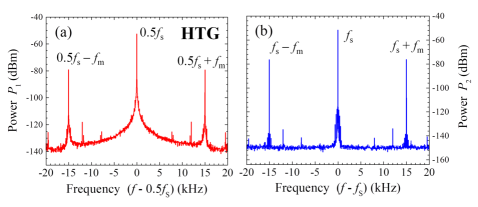
Figure 5: (a) Spectrum of the output signal appeared due to HTG in Sample 2 ($x=d/3$ and $\beta_{L}=0.44$). (b) Spectrum of the amplitude-modulated signal with carrier frequency of $f_{s}=$ 7.76964 GHz $\approx\omega_{2}/2\pi$ = 7.737 GHz and modulation frequency of $f_{m}=15$ kHz applied to the resonator. The spectrum of the generated half tone (a) includes a central peak at frequency $f=f_{s}/2=3.88482$ GHz and two sidebands at frequencies $f_{s}/2\pm f_{m}$. The signal power is $P_{s}=-52$ dBm. The measurements were performed in a helium bath at temperature $T=4.2$ K.

To realize efficient mixing of the two lowest modes, we moved the rf SQUID out of the resonator center, because at $x=0.5d$ mode $n=2$ has a node in the standing-wave of current and, hence, is only weakly coupled to fundamental mode $n=1$. Embedding the rf SQUID at $x=d/3$ yields nonzero values of $|\sin(n\pi x/d)|=|\sin(n\pi/3)|=\sqrt{3}/2$, for all integer $n$ except $n=3,6,9,...$. Then the three-photon coupling coefficient (see Eq. (58) of Appendix B) is

$$B_{lmn} \propto \beta\sin k_{l}x\,\sin k_{m}x\,\sin k_{n}x$$ (12)

$$\approx \beta\sin(l\pi/3)\sin(m\pi/3)\sin(n\pi/3).$$

For modes $l=1$, $m=1$, and $n=2$, the value of $|B_{112}|$ is maximum, while, for example, for modes $l=1$, $m=2$, and $n=3$, its value is zero, $|B_{123}|=0$. The latter property is evident, because the rf SQUID position, $x=d/3$, coincides with the standing-wave node of mode $n=3$ (see the corresponding dashed curve in Fig. 3).

IV.1 Second harmonic generation

Up-conversion (doubling) of the frequency of a light beam while preserving its quantum state Huang1992 is of particular importance in nonlinear optics. A laser beam in this process is usually passing through a large crystal having non-centrosymmetric nonlinearity Boyd2008 . Using of an optical cavity containing a nonlinear crystal and resonant at the second harmonic may enable a source of ultraviolet radiation within this cavity Wu1985 . To demonstrate the intracavity up-conversion of microwaves we applied to the circuit a high frequency drive signal

$$I_{s}(t)=I_{s0}(t)\sin\omega_{s}t$$ (13)

with a slowly oscillating amplitude having the shape

$$I_{s0}(t)=A_{0}(1+\mu\sin\omega_{m}t),$$ (14)

where carrier frequency $\omega_{s}\approx\omega_{1}$, modulation frequency $\omega_{m}\ll\omega_{1,2}/Q_{1,2}\ll\omega_{1}$, $A_{0}=\textrm{const}$, and modulation index $\mu\ll 1$. For sufficiently small driving signal (13), the fundamental-mode oscillations in the cavity have a shape similar to that of the steady-state oscillations in a driven oscillator (see, for example, Ref. Migulin1983 ),

$$I_{1}=I_{0}(t)\sin(\omega_{s}t+\delta+\delta_{0})$$ (15)

with the amplitude

$$I_{0}(t)\propto\frac{I_{s0}(t)}{\sqrt{[1-(\omega_{s}/\omega_{1})^{2}]^{2}+(\omega_{s}/\omega_{1})^{2}/Q_{1}^{2}}}$$ (16)

and phase $\delta$, that is

$$\tan\delta=\frac{\omega_{s}\omega_{1}}{Q_{1}(\omega_{s}^{2}-\omega_{1}^{2})}.$$ (17)

Constant phase $\delta_{0}$ is determined by the parameters of the measuring setup.

The power spectra measured in the vicinities of frequencies $\omega_{s}$ and $2\omega_{s}$ are shown in Fig. 4. One can see the generated frequency triplet consisting of the double frequency carrier at $\omega=2\omega_{s}$ with power $P_{2}$ and two sidebands at frequencies $2\omega_{s}\pm\omega_{m}$ with powers $(\mu^{2}/4)P_{2}$ (see panel (b)). In the time domain, this signal has the shape

$$I_{2}\propto(1+\mu\sin\omega_{m}t)\sin(2\omega_{s}t+\vartheta),$$ (18)

where $\vartheta$ is the relative phase of the generated signal which is coupled to the total phase of the fundamental mode, $\delta+\delta_{0}$. The relatively small output power $P_{2}$ can be explained by rather large frequency mismatch, $(2\omega_{s}-\omega_{2})/2\pi=37.1$ MHz $\gg\omega_{2}/(2\pi Q_{2})\approx 3.86$ MHz, thus the generated signal is off-resonant for the second mode.

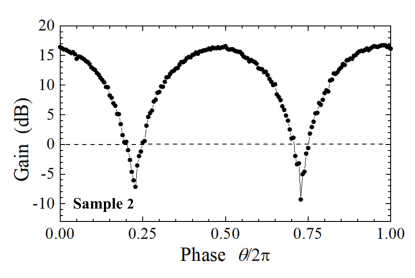
Figure 6: Phase-sensitive parametric amplification and deamplification in Sample 2 (Fig. 3). The input signal frequency and the power are $\omega_{s}/2\pi$ = 3.875 GHz and $-140$ dBm, respectively. The pump frequency and the power are $\omega_{p}/2\pi$ = 7.75 GHz and $-70$ dBm, respectively. The relative phase between these two phase-locked signals is $\theta$ (19). Dashed line shows the level of the output signal power when the pump is off. The maximum signal gain is 17 dB, while the maximum deamplification is about $-8$ dB. The measurements were performed in a dilution refrigerator at temperature $T=18$ mK.

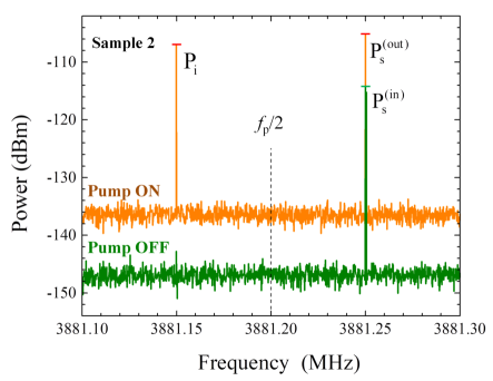
Figure 7: Parametric amplification of signal tone $f_{s}=3.88125$ GHz by means of 3WM in the non-degenerate case (pump frequency $f_{p}=7.7624$ GHz and idler frequency $f_{i}=f_{p}-f_{s}=3.88115$ GHz). The pump power is $P_{p}\approx-65$ dBm. The measurements were performed in a helium bath at $T=4.2$ K.

IV.2 Half tone generation

Applying an intensive harmonic signal with frequency $\omega_{s}$ close to the double resonant frequency of the fundamental mode, $2\omega_{1}\approx\omega_{2}$, may result in HTG, or, equivalently, the oscillation period doubling. (Note that the period tripling was earlier observed in a superconducting resonator with the Kerr nonlinearity by Svensson et al. Svensson2017 .) The period doubling is possible within a finite range of signal frequencies $\omega_{s}$ around $2\omega_{1}$, i.e., $\delta\omega\leq|\omega_{s}/2-\omega_{1}|$. Frequency range $\delta\omega$ depends on the losses for the half tone mode and the signal power that should be sufficient for compensating these losses Migulin1983 . In this case, the zero state of mode $\omega_{1}$ becomes unstable and the circuit switches in one of the oscillating states, both with frequency $\omega_{s}/2$ and the relative phase difference of $\pi$ Zorin2011 .

Figure 5a shows HTG in the case of an amplitude-modulated input signal (13) with $\omega_{s}\approx 2\omega_{1}$, or $\delta\omega\approx 0$, whose power spectrum is presented in Fig. 5b. The output spectrum measured around the half signal frequency, $\omega\sim 0.5\omega_{s}$ (shown in panel (a)) mimics the spectrum of the input signal (panel (b)). It consists of the carrier frequency $(=0.5\omega_{s})$ and two sideband peaks. Due to a very small modulation frequency $(\omega_{m}\ll\omega_{1,2}/Q_{1,2})$ the input signal can be considered as a harmonic signal with a slowly-varying amplitude. Due to the down-conversion (coupling coefficient $B_{211}\neq 0$) and a sufficiently small modulation index, $\mu\ll 1$, the output signal at frequency $\omega=0.5\omega_{s}$ also has an amplitude which is slowly-varying with frequency $\omega_{m}$. Thus, its spectrum presents a triplet, where the small sideband peaks are positioned at $0.5\omega_{s}\pm\omega_{m}$.

Relative phase $\vartheta$ of the generated tone, $I_{\omega_{s}/2}\propto\sin(0.5\omega_{s}t+\vartheta)$, takes randomly one of the two values, $\vartheta=\vartheta_{1,2}$. In the general case, these values depend on the power ($\propto I_{s}^{2}$) and the dissipation in the circuit, but always have a fixed difference, $|\vartheta_{1}-\vartheta_{2}|=\pi$ (see, for example, Eq. (19) in Ref. Zorin2011 ).

IV.3 Parametric amplification

To demonstrate the operation of the circuit in the regime of a Josephson parametric amplifier (JPA) with 3WM in the degenerate mode, we applied a small harmonic signal $I_{s}$ of frequency $\omega_{s}\approx\omega_{1}$ and large pump, $|I_{p}|\gg|I_{s}|$, at the double frequency, $\omega_{p}=2\omega_{s}$, with relative phase difference $\theta$,

$$I_{s}+I_{p}=I_{s0}\sin(\omega_{s}t+\theta)+I_{p0}\sin 2\omega_{s}t.$$ (19)

Figure (6) shows the measured amplification/deamplification versus phase $\theta$. The maximum gain of 17 dB is comparable with the figure reported by Yamamoto et al. Yamamoto2008 for the flux-driven Josephson parametric amplifier based on a $\lambda/4$-cavity terminated by a dc SQUID. The 4WM amplifier of Castellanos-Beltran and Lehnert Castellanos-Beltran2007 , based on a serial array of dc SQUIDs embedded in a $\lambda/4$ CPW resonator, showed a gain slightly above 20 dB. The largest deamplification (about $-8$ dB) measured in our sample is weaker than that achieved in Refs. Yamamoto2008 and Zhong2013 (ca. $-20$ dB). This may be associated with relatively large background noise in our experiment. Still, the observed deamplification can be interpreted as a fingerprint of background-noise squeezing Yurke1989 ; Castellanos-Beltran2008 .

Using the obvious advantage of 3WM, that the frequencies of an intensive pump and a small signal belong to different modes, we have realized the non-degenerate mode of operation of our JPA. The gain in this case is phase preserving. Fixing a small harmonic signal of frequency $\omega_{s}\approx\omega_{1}$ slightly above the half of the pump frequency, $(\omega_{s}-\omega_{p}/2)/2\pi=50~{}\textrm{kHz}<\omega_{1}/Q$, signal gain $G=P^{\textrm{(out)}}_{s}/P^{\textrm{(in)}}_{s}$ of about 9 dB was observed. This direct gain was accompanied by the cross-gain $G_{\textrm{cross}}=P_{i}/P^{\textrm{(in)}}_{s}$ (approximately 8 dB), where the idler at frequency $\omega_{i}=\omega_{p}-\omega_{s}\lesssim\omega_{s}$ has, according to the Manley-Rowe relation Manley-Rowe1956 , the power $P_{i}\lesssim P^{\textrm{(out)}}_{s}$ (see Fig. 7). Both the direct gain $G$ and the cross-gain $G_{\textrm{cross}}$ are proportional to nonlinear coefficient $\beta^{2}$ and, hence, are sensitive to the setting of magnetic flux $\Phi_{e}$.

The latter property together with the periodic dependence of the nonlinear coefficient $\beta$ on the external flux $\Phi_{e}$ with the period of $\Delta\Phi_{e}=\Phi_{0}$, can be used for the evaluation of SQUID-parameter $\beta_{L}$. Using relations (3) and (11) one can find the values of magnetic flux $\Phi_{e}$ giving the maximum of $\beta^{2}$. Within one period, $0\leq\Phi_{e}<\Phi_{0}$, these two values are

$$\Phi_{e1}=\varphi_{0}\arccos(-\beta_{L})+\varphi_{0}\beta_{L}\sqrt{1-\beta^{2}_{L}}$$ (20)

and

$$\Phi_{e2}=\Phi_{0}-\Phi_{e1},$$ (21)

respectively. Note, that the magnetic flux value given by Eq. (20) is somewhat larger than the value given by Eq. (10) for the Kerr-free case, although the difference between these two values is vanishingly small for $\beta_{L}\ll 1$. As long as flux $\Phi_{e}$ is proportional to the control current strength, the ratio $(\Phi_{e2}-\Phi_{e1})/\Phi_{0}=(\Phi_{e2}-\Phi_{e1})/(\Phi_{e2}+\Phi_{e1})$ can be found from the corresponding ratio of the control currents. The above ratio allows finding parameter $\beta_{L}$. Thus, $\beta_{L}$ found in Sample 2 from the parametric cross-gain measurements is 0.446, while the value found from the resonance measurements of this sample is $\beta_{L}=0.44$.

Finally, we note that our open-ended cavity can also operate as a two-mode parametric frequency converter Migulin1983 . (Compare with the ring modulator based on the Wheatstone bridge configuration of four Josephson junctions enabling mixing of the waves in three attached resonators Bergeal2010 .) For example, applying a large pump $(\omega_{p})$ and a small signal $(\omega_{s})$, both with frequencies around $\omega_{1}$, gave rise to generating the sum frequency signal (SFG), $\omega_{\textrm{sum}}=\omega_{s}+\omega_{p}\approx\omega_{2}$. Similarly, the difference frequency generation (DFG), $\omega_{\textrm{dif}}=\omega_{s}-\omega_{p}\approx\omega_{1}$, was also possible, where input signal frequency $\omega_{s}\approx\omega_{2}$, while pump frequency $\omega_{p}\approx\omega_{1}$.

V Discussion and outlook

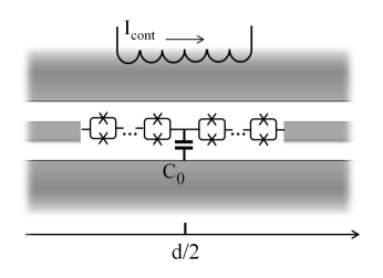
Figure 8: Array of $N$ dc SQUIDs and ground capacitor $C_{0}$ embedded in the central part of the CPW resonator, $x=d/2$. Tuning the reduction of the resonant frequencies of the odd modes is possible by means of constant control current $I_{\textrm{cont}}$ creating a local magnetic field and thus varying the dc SQUID array inductance. A necessary reduction of the resonant frequencies of the even modes occurs due to the ground capacitance $C_{0}$.

In the open-ended cavity with finite coupling capacitances $C_{\textrm{in}}$ and $C_{\textrm{out}}$ and nonzero participation ratio $\alpha$ the resonant frequencies of the modes are not strictly equidistant Goeppl2008 . One can, however, modify the circuit design such that for modes $l=m=1$ and $n=2$ the ratio of the resonant frequencies is 1:2. Then, 3WM condition, $\omega_{l}+\omega_{m}-\omega_{n}=0$, is strictly fulfilled for the first two resonant frequencies of the cavity.

A possible modification of the circuit is shown schematically in Fig. 8, where the array of $N$ dc SQUIDs Palacios-Laloy2008 and a relatively large ground capacitance $C_{0}$ Winkel2020 are embedded in the center of the CPW resonator. As long as the critical current of the Josephson junctions in these dc SQUIDs is relatively large, their Kerr nonlinearity is small. However, the SQUID chain inductance and, thus, the resonant frequencies of all odd modes including $n=1$ (having a current antinode at $x=d/2$) can be varied in a wide range with the help of dc control current $I_{\textrm{cont}}$ Palacios-Laloy2008 . In a similar manner, ground capacitance $C_{0}$ reduces the resonant frequencies of the even modes (having a voltage antinode at $x=d/2$). For a sufficiently large inductance of the dc SQUID chain and a sufficiently large capacitance $C_{0}$, equidistance of all cavity modes with $n\geq 3$ is destroyed, while the frequency ratio for the two lowest modes, $\omega_{2}/\omega_{1}=2$, can be kept fixed by adjusting $I_{\textrm{cont}}$.

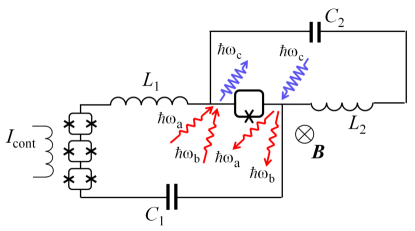
Figure 9: Schematic of a lumped-element circuit comprising two resonators with the ratio of resonant frequencies $\omega_{2}/\omega_{1}=2$ and having nonlinear coupling of $\chi^{(2)}$-type. In the quantum case, this circuit enables SFG with single photons, $\hbar\omega_{a}+\hbar\omega_{b}=\hbar\omega_{c}$, where input frequencies $\omega_{a}\approx\omega_{b}~{}(\approx\omega_{1})$. Under a drive at frequency $\omega_{c}\approx\omega_{2}$, a destruction of photon $\hbar\omega_{c}$ gives rise to creation of the twin photons with frequencies $\omega_{a}\approx\omega_{b}~{}(\approx\omega_{1})$.

The system of two modes tuned in the resonance of type $2\omega_{1}=\omega_{2}$, and having nonlinear coupling of $\chi^{(2)}$ type can be of particular interest in physics Neyfeh1995 . Our CPW cavity with the improved design or its lumped-element analog (see Fig. 9) could be a such a system implemented with the help of superconducting elements and microwave frequencies. For example, if energy losses are negligibly small and a drive is applied to mode $\omega_{1}$ the energy may be periodically transferred from mode $\omega_{1}$ to mode $\omega_{2}$ and vice versa. This behavior mimics the beating-like dynamics of two weakly-coupled identical pendulums Migulin1983 . However, there is a principal difference between these two phenomena; in the case of the circuit with parametric coupling the energy exchange may occur between two oscillators with frequencies being in the ratio of two to one. Similar behavior associated with nonlinear coupling may occur, for example, with the pitch and roll modes of ship motions when the ratio of these frequencies is close to two due to unequal moments of inertia for these two modes Neyfeh1973 .

The superconducting cavity with the predominant coupling of modes $n=1$ and $n=2$ allows for efficient generation of nonclassical states of microwaves. Due to strict phase relations between the input and the output signals, a coherent transfer of the source phase from one part of the spectrum to another is possible. For example, SHG, SFG, and DFG, on the one hand, and HTG and JPA, on the other hand, give rise to quantum frequency conversion (QFC) Shen1984 and spontaneous parametric down-conversion (SPDC) Klyshko1988 , respectively.

In the case of sufficiently low photon-loss rate, $\kappa\ll g$, SFC (with quantum relation $\hbar\omega_{a}+\hbar\omega_{b}=\hbar\omega_{c}$) and SPDC ($\hbar\omega_{c}=\hbar\omega_{a}+\hbar\omega_{b}$) are described by the second quantization Hamiltonian (59) with the relevant part

$$H_{\textrm{nl}}=\hbar g(a_{a}a_{b}a_{c}^{\dagger}+a_{a}^{\dagger}a_{b}^{\dagger}a_{c}).$$ (22)

These processes are schematically shown in Fig. 9. In the case of SFC, the input signals have frequencies $\omega_{a}$ and $\omega_{b}$ around $\omega_{1}$, while the frequency of the output signal, $\omega_{c}\approx\omega_{2}$. In the case of SPDC, the second mode driven at frequency $\omega_{c}\approx\omega_{2}$, gives rise to generating entangled photon pairs within the first mode bandwidth. Thus, the double-mode circuit with $\chi^{(2)}$ nonlinearity can serve as a source of nonclassical microwave light, including squeezed states Movshovich1990 . Note that the three-photon SPDC was recently observed in a microwave-driven superconducting cavity with the Kerr nonlinearity Chang2020 .

VI Conclusion

We have demonstrated that the rf SQUIDs embedded in superconducting coplanar waveguide resonators enabled the observation of a number of remarkable parametric effects. The degree of the non-centrosymmetric nonlinearity, enabling these effects, is governed by the rf SQUID parameter $\beta_{L}$, which value we extracted from resonant frequency modulation. The asymmetric position of this nonlinear element, i.e., at one third of the length of the open-ended resonator, allowed efficient coupling of three waves within the two lowest modes, $n=1$ and $n=2$. The range of observed 3WM processes include SHG, HTG, SFG, DFG, JPA in both degenerate and non-degenerate modes of operation.

The obvious advantage of a resonator with nonlinearity of a $\chi^{(2)}$ type over its counterpart with the Kerr nonlinearity Tancredi2013 is that the former circuit can provide a principally stronger coupling. This property is particularly important for the open-ended resonators, where the intermode coupling is proportional to $\alpha^{2}$ and $\alpha^{3}$, respectively.

In conclusion, we believe that the superconducting cavities with $\chi^{(2)}$ nonlinearity are suitable not only for experiments with classical signals, but also for generating and converting nonclassical states of microwave fields on the level of single photons. In perspective, these circuits may enable nondemolition quantum measurements and quantum computing operations without conventional qubits. The proposed circuit will definitely extend the range of quantum information experiments with microwave photons and thus will have impact on quantum communication technologies.

Appendix A Resonant frequency of a cavity with embedded inductance

A particular solution of a wave equation for the phase variable $\phi(z,t)$ in the lossless open-ended resonator (the coupling capacitances, $C_{\textrm{in}}$ and $C_{\textrm{out}}$, are assumed to be negligibly small), having boundary conditions

$$\frac{\partial\phi(0,t)}{\partial z}=\frac{\partial\phi(d,t)}{\partial z}=0$$ (23)

and embedded inductor $L_{s}$ (positioned not necessarily in the center, as shown in Fig. 1) has the form of a standing-wave,

$$\phi(z,t)=\psi(z)e^{-i\omega_{n}t}.$$ (24)

Here $\omega_{n}$ is the frequency of the $n$-th mode and wave amplitude $\psi(z)$ is a piecewise function whose values for the left and the right segments of the transmission line are given by the harmonic (cosine) functions,

$$\psi(z)=\left\{\begin{array}[]{ll}\psi_{l}(z)=\psi_{a}\cos k_{n}z,&0\leq z<x_{l},\\ \psi_{r}(z)=\psi_{b}\cos[k_{n}(d-z)],&x_{r}<z\leq d.\end{array}\right.$$ (25)

Thus the outer boundary conditions Eq. (23) are fulfilled.

Wave number $k_{n}$ for mode $n=1,2,...$ in the resonator with embedded inductance $L_{s}$ is

$$k_{n}=k^{(0)}_{n}-\delta k_{n},$$ (26)

where the wave number of the bare resonator is Pozar1993

$$k^{(0)}_{n}=n\pi/d$$ (27)

and $\delta k_{n}$ is the change of the wave number due to inductance $L_{s}$. The continuous current conditions on the left and the right terminals of inductance $L_{s}$ read

$$\frac{1}{\ell}\psi_{l}^{\prime}(x_{l})=-\frac{1}{L_{s}}\left[\psi_{l}(x_{l})-\psi_{r}(x_{r})\right]=\frac{\varphi}{L_{s}},$$ (28)

$$\frac{1}{\ell}\psi_{r}^{\prime}(x_{r})=-\frac{1}{L_{s}}\left[\psi_{l}(x_{l})-\psi_{r}(x_{r})\right]=\frac{\varphi}{L_{s}},$$ (29)

where $\varphi$ is the phase drop on inductance $L_{s}$. Using Eq. (25) the derivatives on the left-hand-sides of equations (28) and (29) are expressed as

$$\psi^{\prime}_{l}(x_{l})=-k_{n}\psi_{a}\sin k_{n}x_{l}$$ (30)

and

$$\psi^{\prime}_{r}(x_{r})=k_{n}\psi_{b}\sin[k_{n}(d-x_{r})],$$ (31)

respectively.

Inserting relations (30) and (31) into Eqs. (28) and (29) gives the set of two homogeneous linear equations for wave amplitudes $\psi_{a}$ and $\psi_{b}$,

$$a_{11}\psi_{a}+a_{12}\psi_{b}=0,$$ (32)

$$a_{21}\psi_{a}+a_{22}\psi_{b}=0.$$ (33)

Here coefficients $a_{ij}$ ($i,j=1,2$) are

$$a_{11} = -\alpha k_{n}d\sin k_{n}x_{l}+\cos k_{n}x_{l},$$ (34)

$$a_{12} = -\cos[k_{n}(d-x_{r})],$$ (35)

$$a_{21} = \cos k_{n}x_{l},$$ (36)

$$a_{22} = \alpha k_{n}d\sin[k_{n}(d-x_{r})]-\cos[k_{n}(d-x_{r})],\,\,\,\,\,\,\,\,$$ (37)

where the inductance participation ratio is

$$\alpha=L_{s}/\ell d=L_{s}/L_{\textrm{tot}}.$$ (38)

The condition that the corresponding matrix has a zero determinant and, hence, that a nonzero solution $(\psi_{a},\psi_{b})$ of equations (32) and (33) exists,

$$\Delta=a_{11}a_{22}-a_{12}a_{21}=0,$$ (39)

yields the transcendent equation for wave number $k_{n}$,

$$\alpha k_{n}d\sin k_{n}x_{l}\sin[k_{n}(d-x_{r})]=\sin[k_{n}(d-x_{r}+x_{l})].$$ (40)

Taking into account the fact that both the participation ratio $\alpha$ and the relative size of inductor, $(x_{r}-x_{l})/d=\Delta x/d$ (see Fig. 1a), are small $(\ll 1)$ and, thus, the wave-number change in Eq. (26) is also small, $|\delta k_{n}|\ll n\pi/d$, Eq. (40) is linearized. The resulting simplified equation is

$$(-1)^{n+1}\alpha k_{n}^{(0)}d\sin^{2}k_{n}^{(0)}x=\sin(n\pi-\delta k_{n}d-k_{n}^{(0)}\Delta x)$$ (41)

or

$$\alpha\sin^{2}(n\pi x/d)=\delta k_{n}/k_{n}^{(0)}+\Delta x/d.$$ (42)

Thus the relative shift of the wave number and thus of the resonant frequency for mode $n$ is

$$\frac{\delta k_{n}}{k_{n}^{(0)}}=-\frac{\omega_{n}-\omega^{(0)}_{n}}{\omega^{(0)}_{n}}=\alpha^{*}_{n}\equiv\alpha\sin^{2}\frac{n\pi x}{d}-\frac{\Delta x}{d}.$$ (43)

Here the trigonometric factor $\sin^{2}(n\pi x/d)$ gives the dependence on the inductor position $x$, while term $\Delta x/d$ describes the effective reduction of the resonator length, $d\rightarrow d-\Delta x$. The resulting eigenfrequencies are

$$\omega_{n}=\omega^{(0)}_{n}(1-\alpha_{n}^{*}),~{}~{}~{}~{}n=1,2,3,...$$ (44)

and wave numbers are

$$k_{n}=n\pi d\,(1-\alpha_{n}^{*}).$$ (45)

The corresponding eigensolutions of the homogeneous wave equation in the range $0\leq z\leq d$ have the form

$$\psi_{n} = [1-\alpha\pi n(-1)^{n}]\,\Theta(x_{l}-z)\cos k_{n}z$$ (46)

$$+ \Theta(z-x_{r})\cos[k_{n}(d-z)]\approx\cos k_{n}z,$$

where $\Theta(z)$ is the Heaviside step function.

Appendix B Two-mode Hamiltonian of the cavity with $\chi^{(2)}$ nonlinearity

The rf SQUID potential energy in the case of the optimal flux bias, $\Phi_{\textrm{dc}}=\Phi_{0}/4$ (or $\varphi_{\textrm{dc}}=\Phi_{\textrm{dc}}/\varphi_{0}=\pi/2$), and small ac phase difference on the Josephson junction, $|\varphi|\ll\pi/2$, is given by

$$E_{s}=\varphi_{0}\int^{\varphi}I(\varphi)d\varphi=E_{s0}\left(\frac{\varphi^{2}}{2}-\beta\frac{\varphi^{3}}{3}\right),$$ (47)

where energy $E_{s0}=\varphi^{2}_{0}/L_{g}$. The first term ($\propto\varphi^{2}$) on the right hand side of this relation contributes only to the eigenmode frequency Eq. (44). Omitting, for a moment, the nonlinearity of the rf SQUID, the Hamiltonian of the resonator can be presented using the second quantization formalism in the standard form,

$$H_{0}=\sum_{n=1}^{\infty}\hbar\omega_{n}a_{n}^{\dagger}a_{n},$$ (48)

where $a^{\dagger}_{n}$ and $a_{n}$ are creation and annihilation operators of the $n$-th mode, respectively.

The last term on the right hand side of Eq. (47), that is

$$E_{\textrm{nl}}=-\frac{1}{3}\beta E_{s0}\varphi^{3}=-\frac{1}{3}\beta\alpha^{3}E_{s0}d^{3}\,(\phi^{\prime})^{3},$$ (49)

describes the energy associated with the rf SQUID nonlinearity. Here the inductance participation ratio is $\alpha=L_{g}/L_{\textrm{tot}}\ll 1$ and phase $\varphi$ is expressed via derivative $\phi^{\prime}$ using Eqs. (28) and (29). Using the normal-mode decomposition of phase $\phi$ Eichler2014 ,

$$\phi=\sum_{n=1}^{\infty}A_{n}\psi_{n}=\sum_{n=1}^{\infty}A_{n}\cos k_{n}x,$$ (50)

the nonlinear part of the rf SQUID energy takes the form

$$E_{\textrm{nl}}=\sum_{l,m,n=1}^{\infty}B_{lmn}A_{l}A_{m}A_{n},$$ (51)

where

$$B_{lnm}=\frac{1}{3}\beta\alpha^{3}E_{s0}\prod_{j\in\{l,m,n\}}k_{j}d\,\sin k_{j}x.$$ (52)

In the quantum case, the coefficients in the normal-mode decomposition Eq. (50) are operators, $A_{n}\rightarrow\hat{A}_{n}$. They can be expressed via annihilation ($a_{n}$) and creation ($a^{\dagger}_{n}$) boson operators Wallquist2006 , that is

$$\hat{A}_{n}=\phi_{\textrm{zpf},n}(a^{\dagger}_{n}+a_{n}),$$ (53)

where the prefactor is associated with the magnitude of zero-point fluctuations Eichler2014 ; Girvin2011 ,

$$\phi_{\textrm{zpf},n}=\varphi_{0}^{-1}\sqrt{\hbar/2\omega_{n}C_{\textrm{eff},n}}.$$ (54)

Using the bare cavity values of frequencies $\omega_{n}$ (6) and capacitances $C_{\textrm{eff},n}$ (8) we have

$$\phi_{\textrm{zpf},n}\approx\sqrt{\frac{2Z_{0}}{nR_{Q}}}\approx\frac{0.124}{\sqrt{n}},$$ (55)

where impedance $Z_{0}=\sqrt{L_{\textrm{tot}}/C_{\textrm{tot}}}=50~{}\Omega$ and resistance quantum $R_{Q}=h/4e^{2}\approx 6.45~{}\textrm{k}\Omega$. Inserting Eq. (53) in expression (51) yields nonlinear part of Hamiltonian $H_{\textrm{nl}}$ in terms of operators $a_{n}$ and $a^{\dagger}_{n}$.

Applying a rotating wave approximation and thus omitting all oscillating terms of type $a_{l}a_{m}a_{n}$, $a^{\dagger}_{l}a^{\dagger}_{m}a^{\dagger}_{n}$, etc., we keep only terms $a_{l}a_{m}a^{\dagger}_{n}$ and $a^{\dagger}_{l}a^{\dagger}_{m}a_{n}$ with the frequencies obeying the three photon (3WM) relation,

$$\omega_{l}+\omega_{m}-\omega_{n}=0,~{}~{}~{}\textrm{or},~{}~{}~{}l+m-n=0.$$ (56)

we obtain the total Hamiltonian, $H=H_{0}+H_{\textrm{nl}}$, in the form

$$\frac{H}{\hbar}=\sum_{n=1}^{\infty}\omega_{n}a_{n}^{\dagger}a_{n}+\sum_{l+m-n=0}g_{lmn}(a_{l}a_{m}a_{n}^{\dagger}+a_{l}^{\dagger}a_{m}^{\dagger}a_{n}),$$ (57)

where the mode coupling coefficient is

$$g_{lmn}=\frac{1}{\hbar}\left(\frac{2Z_{0}}{R_{Q}}\right)^{3/2}\sqrt{lmn}\,B_{lmn}.$$ (58)

Assuming that relation (56) is fulfilled only for the two lowest modes, i.e., $\omega_{2}=2\omega_{1}$, Hamiltonian (57) takes the form

$$H=\sum_{n=1}^{2}\hbar\omega_{n}a_{n}^{\dagger}a_{n}+\hbar g(a_{1}a_{1}a_{2}^{\dagger}+a_{1}^{\dagger}a_{1}^{\dagger}a_{2}),$$ (59)

where

$$\hbar g=3\hbar g_{112}=\beta\alpha^{3}\left(\frac{3Z_{0}}{R_{Q}}\right)^{3/2}E_{s0}$$ (60)

or

$$\frac{g}{\omega_{1}}=\frac{3\beta\alpha^{2}}{2\pi^{2}}\sqrt{\frac{3Z_{0}}{R_{Q}}}.$$ (61)

Here we used the relations $g_{112}=g_{121}=g_{211}\equiv g/3$ and $\sin k_{1}d=\sin k_{2}d\approx\sqrt{3}/2$ and the commutative property of the operators associated with different modes, $[a_{1},a_{2}^{\dagger}]=[a_{1}^{\dagger},a_{2}]=0$.

Appendix C Sample measurements

The samples were characterized using a vector network analyzer (VNA) R$\&$S ZVA 40 by measuring transmission through the CPW resonator (parameters $S21$ and $b2$) as a function of frequency and/or microwave power. In the mixing experiments a microwave power supply was made using the sources R$\&$S SMF100A, while an output power was measured by a spectrum analyzer (R$\&$S FSV 30). In the experiments in liquid helium, the chips were bonded on a printed circuit board with the SMA connectors and mounted in a metallic box. In the dilution fridge unit, the attenuators in the input rf line mounted at different temperature stages gave an attenuation of $-50$ dB in total (including attenuation in the cables). In the output rf line, two circulators (with the bandwidth of $3.2-8.1$ GHz) were installed at the mixing chamber level. The input and output rf lines (coaxial cables) were directly bonded to the chip. The flux bias lines were supplied with the on-chip low-pass filters comprising the spiral-shape Nb coils with inductance about 5.5 nH. In both setups the sample was protected by a cryoperm shield. The readout of the output signal was done using a semiconductor low-noise amplifier from Low Noise Factory, model LNF-LNC0.3-14A. It operated in the range of 0.3-14 GHz with a gain up to 40 dB and a noise temperature of about 5 K. This cryogenic amplifier was installed at the 4 K stage of the dilution fridge unit.

References

- (1) M. A. Castellanos-Beltran and K. W. Lehnert, Widely tunable parametric amplifier based on a superconducting quantum interference device array resonator, Appl. Phys. Lett. 91, 083509 (2007).
- (2) T. Yamamoto, K. Inomata, M. Watanabe, K. Matsuba, T. Miyazaki, W. D. Oliver, Y. Nakamura, and J. S. Tsai, Flux-driven Josephson parametric amplifier, Appl. Phys. Lett. 93, 042510 (2008).
- (3) C. Eichler, D. Bozyigit, C. Lang, M. Baur, L. Steffen, J. M. Fink, S. Filipp, and A. Wallraff, Observation of two-mode squeezing in the microwave frequency domain, Phys. Rev. Lett. 107, 113601 (2011).
- (4) V. E. Manucharyan, E. Boaknin, M. Metcalfe, R. Vijay, I. Siddiqi, and M. Devoret, Microwave bifurcation of a Josephson junction: Embedding-circuit requirements, Phys. Rev. B 76, 014524 (2007).
- (5) M. Metcalfe, E. Boaknin, V. Manucharyan, R. Vijay, I. Siddiqi, C. Rigetti, L. Frunzio, R. J. Schoelkopf, and M. H. Devoret, Measuring the decoherence of a quantronium qubit with the cavity bifurcation amplifier, Phys. Rev. B 76, 174516 (2007).
- (6) R. Vijay, M.H. Devoret, and I. Siddiqi, Invited review article: The Josephson bifurcation amplifier, Rev. Sci. Instrum. 80, 111101 (2009).
- (7) G. Tancredi, G. Ithier, and P. Meeson. Bifurcation, mode coupling and noise in a nonlinear multimode superconducting microwave resonator. Appl. Phys. Lett. 103, 063504 (2013).
- (8) W. Wustmann and V. Shumeiko, Parametric resonance in tunable superconducting cavities, Phys. Rev. B 87, 184501 (2013).
- (9) M. A. Castellanos-Beltran, K. Irwin, G. Hilton, L. Vale, and K. Lehnert, Amplification and squeezing of quantum noise with a tunable Josephson metamaterial, Nat. Phys. 4, 928 (2008).
- (10) L. Zhong, E. P. Menzel, R. Di Candia, P. Eder, M. Ihmig, A. Baust, M. Haeberlein, E. Hoffmann, K. Inomata, T. Yamamoto, Y. Nakamura, E. Solano, F. Deppe, A. Marx, and R. Gross, Squeezing with a flux-driven Josephson parametric amplifier, New J. Phys. 15, 125013 (2013).
- (11) B. H. Schneider, A. Bengtsson, I. M. Svensson, T. Aref, G. Johansson, J. Bylander, and P. Delsing, Observation of broadband entanglement in microwave radiation from a single time-varying boundary condition, Phys. Rev. Lett. 124, 140503 (2020).
- (12) C.M. Wilson, G. Johansson, A. Pourkabirian, M. Simoen, J. R. Johansson, T. Duty, F. Nori, and P. Delsing, Observation of the dynamical Casimir effect in a superconducting circuit, Nature 479, 376 (2011).
- (13) P. Lahteenmäki, G. S. Paraoanu, J. Hassel, and P. J. Hakonen, Dynamical Casimir effect in a Josephson metamaterial, PNAS 110, 4234 (2013).
- (14) C. W. S. Chang, C. Sabín, P. Forn-Díaz, F. Quijandría , A. M. Vadiraj, I. Nsanzineza, G. Johansson, and C. M. Wilson, Observation of three-photon spontaneous parametric down-conversion in a superconducting parametric cavity, Phys. Rev. X 10, 011011 (2020).
- (15) A. Palacios-Laloy, F. Nguyen, F. Mallet, P. Bertet, D. Vion, and D. Esteve, Tunable Resonators for Quantum Circuits, J. Low Temp. Phys. 151, 1034 (2008).
- (16) J. Bourassa, F. Beaudoin, Jay M. Gambetta, and A. Blais, Josephson-junction-embedded transmission-line resonators: From Kerr medium to in-line transmon, Phys. Rev. A 86, 013814 (2012).
- (17) C. Eichler and A. Wallraff, Controlling the dynamic range of a Josephson parametric amplifier, EPJ Quantum Technol. 1, 2 (2014).
- (18) M.H. Devoret and R.J. Schoelkopf, Superconducting circuits for quantum information: An outlook, Science 339, 1169 (2013).
- (19) Y. R. Shen, The principles of nonlinear optics (Wiley, New York, 1984).
- (20) B. Yurke, L. R. Corruccini, P. G. Kaminsky, L. W. Rupp, A. D. Smith, A. H. Silver, R. W. Simon, and E. A. Whittaker, Observation of parametric amplification and deamplification in a Josephson parametric amplifier, Phys. Rev. A 39, 2519 (1989).
- (21) A. B. Zorin, Josephson traveling-wave parametric amplifier with three-wave mixing, Phys. Rev. Applied 6, 034006 (2016).
- (22) A. B. Zorin, M. Khabipov, J. Dietel, and R. Dolata, Traveling-wave parametric amplifier based on three-wave mixing in a Josephson metamaterial, 2017 16th International Superconductive Electronics Conference (ISEC), Naples, 2017, pp. 1-3, doi: 10.1109/ISEC.2017.8314196.
- (23) N. E. Frattini, U. Vool, S. Shankar, A. Narla, K. M. Sliwa, and M. H. Devoret, 3-wave mixing Josephson dipole element, Appl. Phys. Lett. 110, 222603 (2017).
- (24) S. K. Kurtz and T. T. Perry, A powder technique for the evaluation of nonlinear optical materials, J. Appl. Phys. 39, 3798 (1968).
- (25) G. P. Agrawal, Nonlinear fiber optics (Academic press, San Diego, California, 2007).
- (26) A. Miano and O. A. Mukhanov, Symmetric traveling wave parametric amplifier, IEEE Trans. Appl. Supercond. 29, 1501706 (2019).
- (27) S. Ó Peatáin, T. Dixon, P. J. Meeson, J. M. Williams, S. Kafanov, and Y. A. Pashkin, The effect of parameter variations on the performance of the Josephson travelling wave parametric amplifiers, arXiv:2112.07766.
- (28) V.V. Sivak, N.E. Frattini, V.R. Joshi, A. Lingenfelter, S. Shankar, and M.H. Devoret, Kerr-free three-wave mixing in superconducting quantum circuits, Phys. Rev. Applied 11, 054060 (2019).
- (29) N. E. Frattini, V. V. Sivak, A. Lingenfelter, S. Shankar, and M. H. Devoret, Optimizing the nonlinearity and dissipation of a SNAIL parametric amplifier for dynamic range, Phys. Rev. Applied 10, 054020 (2018).
- (30) A. Miano, G. Liu, V. V. Sivak, N. E. Frattini, V. R. Joshi, W. Dai, L. Frunzio, and M. H. Devoret, Frequency-tunable Kerr-free three-wave mixing with a gradiometric SNAIL, arXiv:2112.09785.
- (31) V. V. Sivak , S. Shankar, G. Liu, J. Aumentado, and M. H. Devoret, Josephson array-mode parametric amplifier, Phys. Rev. Applied 13, 024014 (2020).
- (32) F. Wulschner, J. Goetz, F. R. Koessel, E. Hoffmann, A. Baust, P. Eder, M. Fischer, M. Haeberlein, M. J. Schwarz, M. Pernpeintner, E. Xie, L. Zhong, C. W. Zollitsch, B. Peropadre, J.-J. G. Ripoll, E. Solano, K. G. Fedorov, E. P. Menzel, F. Deppe, A. Marx, and R. Gross, Tunable coupling of transmission-line microwave resonators mediated by an rf SQUID, EPJ Quantum Technol. 3, 10 (2016).
- (33) M. S. Allman, J. D. Whittaker, M. Castellanos-Beltran, K. Cicak, F. da Silva, M. P. DeFeo, F. Lecocq, A. Sirois, J. D. Teufel, J. Aumentado, and R. W. Simmonds, Tunable resonant and nonresonant interactions between a phase qubit and LC resonator, Phys. Rev. Lett. 112, 123601 (2014).
- (34) M. Göppl, A. Fragner, M. Baur, R. Bianchetti, S. Filipp, J. M. Fink, P. J. Leek, G. Puebla, L. Steffen, and A. Wallraff, Coplanar waveguide resonators for circuit quantum electrodynamics, J. Appl. Phys. 104, 113904 (2008).
- (35) J. M. Martinis, K. B. Cooper, R. McDermott, M. Steffen, M. Ansmann, K. D. Osborn, K. Cicak, S. Oh, D. P. Pappas, R. W. Simmonds, and C. C. Yu, Decoherence in Josephson qubits from dielectric loss, Phys. Rev. Lett. 95, 210503 (2005).
- (36) J. Burnett, L. Faoro, and T. Lindström, Analysis of high quality superconducting resonators: consequences for TLS properties in amorphous oxides, Supercond. Sci. Technol. 29, 044008 (2016).
- (37) S. E. de Graaf, L. Faoro, L. B. Ioffe, S. Mahashabde, J. J. Burnett, T. Lindström, S. E. Kubatkin, A. V. Danilov, and A. Ya. Tzalenchuk, Two-level systems in superconducting quantum devices due to trapped quasiparticles, Sci. Adv. 6, eabc5055 (2020).
- (38) M. P. Weides, J. S. Kline, M. R. Vissers, M. O. Sandberg, D. S. Wisbey, B. R. Johnson, T. A. Ohki, and D. P. Pappas, Coherence in a transmon qubit with epitaxial tunnel junctions, Appl. Phys. Lett. 99, 262502 (2011).
- (39) R. Dolata, H. Scherer, A. B. Zorin, and J. Niemeyer, Single-charge devices with ultrasmall Nb/AlOx/Nb trilayer Josephson junctions, J. Appl. Phys. 97, 054501 (2005).
- (40) M. Khabipov, B. Mackrodt, R. Dolata, T. Scheller, and A. Zorin, Investigation of nonlinear superconducting microwave resonators including Nb Josephson junctions and SQUID arrays, J. Phys.: Conf. Ser. 507, 042016 (2014).
- (41) K. K. Likharev, Dynamics of Josephson junctions and circuits (Gordon and Breach, New York, 1986).
- (42) R. Rifkin and B. S. Deaver, Jr., Current-phase relation and phase-dependent conductance of superconducting point contacts from rf impedance measurements, Phys. Rev. B 13, 3894 (1976).
- (43) E. Il’ichev, V. Zakosarenko, L. Fritzsch, R. Stolz, H. E. Hoenig, H.-G. Meyer, M. Götz, A. B. Zorin, V. V. Khanin, A. B. Pavolotsky, and J. Niemeyer, Radio-frequency based monitoring of small supercurrents, Rev. Sci. Instrum. 72, 1882 (2001).
- (44) M. Wegner, C. Enss, and S. Kempf, Analytical model of the readout power and SQUID hysteresis parameter dependence of the resonator characteristics of microwave SQUID multiplexers, arXiv:2112.08278.
- (45) D. M. Pozar, Microwave Engineering (Wiley, 2012).
- (46) M. Wallquist, V. S. Shumeiko, G. Wendin, Selective coupling of superconducting charge qubits mediated by a tunable stripline cavity, Phys. Rev. B 74, 224506 (2006).
- (47) V. Ambegaokar and A. Baratoff, Tunneling between superconductors, Phys. Rev. Lett. 10, 486 (1963).
- (48) J. Huang and P. Kumar, Observation of quantum frequency conversion, Phys. Rev. Lett. 68, 2153 (1992).
- (49) R. W. Boyd, Nonlinear optics (Academic Press, London, 2008).
- (50) Ling-An Wu and H. J. Kimble, Interference effects in second-harmonic generation within an optical cavity, J. Opt. Soc. Am. B 2, 697 (1985).
- (51) V. Migulin, V. Medvedev, E. Mustel, and V. Parygin, Basic theory of oscillations (Mir Publishers, Moscow, 1983).
- (52) I.-M. Svensson, A. Bengtsson, P. Krantz, J. Bylander, V. Shumeiko, and P. Delsing, Period-tripling subharmonic oscillations in a driven superconducting resonator, Phys. Rev. B 96, 174503 (2017).
- (53) A. B. Zorin and Y. Makhlin, Period-doubling bifurcation readout for a Josephson qubit, Phys. Rev. B 83, 224506 (2011).
- (54) J. M. Manley and H. E. Rowe, Some general properties of nonlinear elements, part 1. General energy relations, Proc. IRE 44, 904 (1956).
- (55) N. Bergeal, F. Schackert, M. Metcalfe, R. Vijay, V. E. Manucharyan, L. Frunzio, D. E. Prober, R. J. Schoelkopf, S. M. Girvin, and M. H. Devoret, Phase-preserving amplification near the quantum limit with a Josephson ring modulator, Nature 465, 64 (2010).
- (56) P. Winkel, I. Takmakov, D. Rieger, L. Planat, W. Hasch-Guichard, L. Grunhaupt, N. Maleeva, F. Foroughi, F. Henriques, K. Borisov, J. Ferrero, A. V. Ustinov, W. Wernsdorfer, N. Roch, and I. M. Pop, Nondegenerate parametric amplifiers based on dispersion-engineered Josephson-junction arrays, Phys. Rev. Applied 13, 024015 (2020).
- (57) A. H. Neyfeh and D. T. Mook, Nonlinear oscillations (Wiley, New York, 1995).
- (58) A. H. Neyfeh, D. T. Mook, and L. R. Marshall, Nonlinear coupling of pitch and roll modes in ship motion, J. Hydronautics 7, 145 (1973).
- (59) D. N. Klyshko, Photons and nonlinear optics (Gordon and Breach, New York, 1988).
- (60) R. Movshovich, B. Yurke, P. G. Kaminsky, A. D. Smith, A. H. Silver, R. W. Simon, and M. V. Schneider, Observation of zero-point noise squeezing via a Josephson-parametric amplifier, Phys. Rev. Lett. 65, 1419 (1990).
- (61) S. M. Girvin, Superconducting qubits and circuits: Artificial atoms coupled to microwave photons (Lectures delivered at École d’Été, Les Houches, Oxford University Press, 2011).