Short-time asymptotics for non self-similar
stochastic volatility models

Giacomo Giorgio giorgio@mat.uniroma2.it Department of Mathematics, University of Rome Tor Vergata, Roma, Italy. Barbara Pacchiarotti pacchiar@mat.uniroma2.it Department of Mathematics, University of Rome Tor Vergata, Roma, Italy. Paolo Pigato paolo.pigato@uniroma2.it Department of Economics and Finance, University of Rome Tor Vergata, Roma, Italy.
(March 11, 2024)
Abstract

We provide a short-time large deviation principle (LDP) for stochastic volatility models, where the volatility is expressed as a function of a Volterra process. This LDP does not require strict self-similarity assumptions on the Volterra process. For this reason, we are able to apply such an LDP to two notable examples of non self-similar rough volatility models: models where the volatility is given as a function of a log-modulated fractional Brownian motion [Bayer et al., Log-modulated rough stochastic volatility models. SIAM J. Financ. Math, 2021, 12(3), 1257-1284], and models where it is given as a function of a fractional Ornstein-Uhlenbeck (fOU) process [Gatheral et al., Volatility is rough. Quant. Finance, 2018, 18(6), 933-949]. In both cases we derive consequences for short-maturity European option prices, implied volatility surfaces and implied volatility skew. In the fOU case we also discuss moderate deviations pricing and simulation results.

Keywords: rough volatility, stochastic volatility, implied volatility, European option pricing, short-time asymptotics, fractional Brownian motion, fractional Ornstein-Uhlenbeck, modulated models, Volterra processes.

2020 Mathematics Subject Classification: 91G20, 60H30, 60F10, 60G22.

JEL Classifications: C32, C63, G12.

Acknowledgements: We are grateful to Christian Bayer, Lucia Caramellino for discussion and support. Barbara Pacchiarotti acknowledges the support of Indam-GNAMPA (research project “Stime asintotiche: principi di invarianza e grandi deviazioni”), of the MIUR Excellence Department Project awarded to the Department of Mathematics, University of Rome Tor Vergata (CUP E83C18000100006) and of University of Rome Tor Vergata (research program “Beyond Borders”, project “Asymptotic Methods in Probability”(CUP E89C20000680005)).

1 Introduction

Recent years have seen wide interest in volatility modelling with Volterra processes in the quantitative finance community. This has been spurred by the success of rough volatility models, where volatility is a non-Markovian, fractional process (Gatheral et al., 2018). In many instances, in order to produce this type of dynamics, volatility is expressed as a function of a Volterra process, i.e. a suitable deterministic kernel integrated against a Brownian motion. In this context a very useful feature of such kernel and of the corresponding fractional process is self-similarity.

When looking at approximation formulas and asymptotics, self-similarity is usually key as it enables the translation of a small-noise result into a short-time one through space-time rescaling. This can then be used to price short maturity options (see the discussion at the end of Section 3 in Gulisashvili (2020), and Gulisashvili (2018)). Based on this procedure, several short-time formulas are available for rough volatility models, if the volatility process is expressed as a function of a fractional Brownian motion (fBM) (Forde and Zhang, 2017), as a function of a Riemann-Liouville process (RLp), as in the rough Bergomi model (Bayer et al., 2019; Friz et al., 2022; Fukasawa, 2020), or as a solution to a fractional SDE, as in the fractional Heston model (Forde et al., 2021).

However, obtaining short-time approximation formulas is more difficult if volatility depends on a process which is not self-similar, such as the fractional Ornstein-Uhlenbeck (fOU) process (Horvath et al., 2019; Garnier and Sølna, 2017, 2018a, 2020b, 2019, 2020a), or the log-modulated fBM (log-fBM) (Bayer et al., 2021). In this paper, we address this issue, providing a short-time large deviation principle (LDP) for Volterra-driven stochastic volatilities, where the usual self similarity assumption is replaced by a weaker scaling property for the kernel, that needs to hold only in asymptotic sense (see conditions (K1) and (K2) below). We prove this general result starting from (Cellupica and Pacchiarotti, 2021), where a pathwise LDP for the log-price was proved when the volatility is function of a family of Volterra processes, and the price is solution to a scaled differential equation. Here, under suitable short-time asymptotic assumptions on the Volterra kernel, we prove a short-time LDP for the log-price process.

With our general result, we analyse more in depth models with volatility given as a function of fOU or log-fBM, neither of which is self-similar. However, we note that both these processes can be seen as a perturbation of self-similar processes, so that our general result can be applied, assuming that the price process is a martingale and a moment condition on the price.

The first class of processes to which we apply our LDP are log-modulated rough stochastic volatility models, introduced in Bayer et al. (2021) as a logarithmic perturbation of a more standard power-law Volterra stochastic volatility model, with volatility depending on a log-fBM. These models allow for the definition of a “true”, continuous volatility process with roughness (Hurst) parameter H[0,1]𝐻01H\in[0,1] (including the “super-rough” case H=0𝐻0H=0), at the price of losing the self-similar structure of the power-law kernel. Differently from our LDP setting, however, in Bayer et al. (2021) Edgeworth-type asymptotics are considered, meaning that log-moneyness is of the form xt𝑥𝑡x\sqrt{t} (t𝑡t representing the time to maturity), while in order to observe a large deviations behavior we look here at a suitable log-moneyness regime (cf. equation (4.2)). This regime is consistent with Forde-Zhang LDP for rough volatility (Forde and Zhang, 2017) and the related large deviation results discussed below. When H>0𝐻0H>0, we obtain a short-time LDP for the log-price process and consequent short-time option pricing, implied volatility and implied skew asymptotics. For this class of processes the rate function only depends on the self-similar power-law kernel, while the speed depends also on the modulating logarithmic function. It is shown in Bayer et al. (2021) that when H=0𝐻0H=0 the implied volatility skew explodes as t1/2superscript𝑡12t^{-1/2} (with a logarithmic correction), realising the model free bound in Lee (2005). Even though our proof only holds in the H>0𝐻0H>0 case, the expression we obtain for skew asymptotics, computed for H=0𝐻0H=0, is consistent with this model free bound. We note that Baldi and Pacchiarotti (2022) have recently proved that in the H=0𝐻0H=0 case, even if the log-modulated model is well defined, an LDP cannot hold.

The second class of models to which we apply our LDP have a stochastic volatility given by a function of a fractional Ornstein-Uhlenbeck process. We find that, in short-time, such model behaves exactly as the analogous model, with volatility process given as the same function, computed on a fBM (i.e., the model studied in Forde and Zhang (2017)). More precisely, we mean that the two models satisfy an LDP with same speed and rate function. It follows that also the short-time implied skew (computed as a suitable finite difference) is the same for fOU and fBM-driven stochastic volatility models. For small time scales, fOU is, in a sense, close to fBM (see equation (3.6)), even though fOU is not self-similar. It is not uncommon when dealing with rough stochastic volatility, starting from the groundbreaking work Gatheral et al. (2018), to consider at times fBM, at times fOU, depending on which is most convenient for the problem at hand. Our result can be seen as a justification of this type of procedure, as it shows that pricing vanilla options with one or the other volatility does not matter (too much) for short maturities. Moreover, the fOU process is the most standard choice for a stationary process with a fractional correlation structure. This is one of the reasons why it has been used as volatility process for option pricing and related issues111note that both fBM and RLp (as in Rough Bergomi) are non-stationary and give rise to non-stationary volatility processes (Horvath et al., 2019; Garnier and Sølna, 2017, 2018a, 2020b, 2019, 2020a).

From our short-time LDP we formally derive the corresponding moderate deviations result, consistent with the one holding for self-similar rough volatility (Bayer et al., 2019). We provide numerical evidence for both these large and moderate deviations results and for the skew asymptotics. We investigate on simulations how the choice between fOU and fBM dynamics in the volatility affects volatility smiles and skews, how accurate are our approximations, and how they depend on the mean reversion parameter.

Background. In recent years, rough volatility has been widely used in option pricing, due to the great fits it provides to observed volatility surfaces (Bayer et al., 2016) and its ability to capture fundamental stylized facts of the implied volatility, notably the power-law explosion of the implied skew in short-time, which explodes as tH1/2superscript𝑡𝐻12t^{H-1/2} under rough volatility (Alòs et al., 2007; Fukasawa, 2011, 2017). Many authors have argued that H𝐻H is actually positive but very close to 00 (Bayer et al., 2016; Fukasawa, 2020), which would give an extreme skew explosion close to t1/2superscript𝑡12t^{-1/2}. This is a model-free bound (Lee, 2005), that can be reached pricing options using “singular” local (or local-stochastic) volatility models (Pigato, 2019; Friz et al., 2021), but it is hard to obtain with (rough) stochastic volatility, as in the limit H0𝐻0H\to 0 the volatility process usually degenerates and can be defined only as a distribution, not as a genuine process (Forde et al., 2020, 2021; Neuman and Rosenbaum, 2018; Hager and Neuman, 2021). Moreover, one observes a skew-flattening phenomenon, as H0𝐻0H\to 0, in some of these models. This was the main motivation, in Bayer et al. (2021), to introduce the log-modulation of the power law kernel, allowing the corresponding stochastic volatility to be defined as a genuine process also in the H0𝐻0H\to 0 limit. Technically, the logarithmic correction ensures that the variance remains finite even for H=0𝐻0H=0, that in turn avoids the subsequent definition problems as H0𝐻0H\to 0, as well as the skew-flattening problem. We refer to Bayer et al. (2021) and references therein for a detailed discussion of the H0𝐻0H\to 0 problem.

Volatility was already taken as an exponential function of a fOU process with H<1/2𝐻12H<1/2 when rough volatility was first proposed in Gatheral et al. (2018). On the one hand, mostly because of the desired self-similarity property of the volatility process, the exponential of a fBM or of a RLp222RLp is the stochastic process driving the volatility in the rough Bergomi model (Bayer et al., 2016), are often used for pricing options. On the other hand, it is argued, e.g. in Gatheral et al. (2018), that taking a fOU with small mean reversion is not very different from taking a fBM in the volatility, with the considerable advantage that fOU is a stationary process (Cheridito et al., 2003), while fBM and RLp are not. For a thorough discussion on fOU driven volatilities and related implied volatilities we refer in particular to Garnier and Sølna (2017, 2020a), for the relation of fOU to fast mean reverting Markov stochastic volatility we refer to Garnier and Sølna (2018a, 2019), for hedging under fOU volatility we refer to Garnier and Sølna (2020b), for portfolio optimization using fast mean reverting fOU process with H>1/2𝐻12H>1/2 we refer to Fouque and Hu (2018). A small-noise LDP under fOU volatility, with other related results, has been proved in Horvath et al. (2019), and LDP and moderate deviation principles for the rough Stein-Stein and other models, also in short-time, have been discussed in Jacquier and Pannier (2022) (see Remark 4.9 for details).

In this paper we consider short-time pricing asymptotics, i.e. pricing short maturity European options. This is a widely studied topic, as these short maturity pricing formulas provide methods for fast calibration, a quantitative understanding of the impact of model parameters on generated implied volatility surfaces, led to some widely used parametrizations of the volatility surface, and help in the choice of the most appropriate model to be fitted to data (Ait-Sahalia et al., 2020). Short maturity approximations are also used to obtain starting points for calibration procedures, which are then based on numerical evaluations. They have applications also to hedging, trading and risk management.

For notable results on short maturity valuation formulas under Markovian stochastic volatility we refer to Osajima (2015), and to Medvedev and Scaillet (2003, 2007) for Markovian stochastic volatility with jumps. Short-time skew and curvature under rough volatility have been discussed in Fukasawa (2017); Alòs and Leon (2017). Short maturity valuation formulas for European options and implied volatilities under rough stochastic volatility are given, e.g., in Forde and Zhang (2017); El Euch et al. (2019); Bayer et al. (2019); Friz et al. (2021, 2022); Fukasawa (2020). Short maturity local volatility under rough volatility is studied in Bourgey et al. (2023). Pathwise large and moderate deviation principles for rough stochastic volatility models are established in Horvath et al. (2019); Jacquier et al. (2018); Jacquier and Pannier (2022); Gulisashvili (2018, 2020, 2021, 2022); Gulisashvili et al. (2018a, b); Cellupica and Pacchiarotti (2021); Catalini and Pacchiarotti (2023).

Content of the paper. We consider in Section 2 an LDP for stochastic volatility models with volatility driven by general Volterra processes. In particular, in Section 2.2 we prove a short-time LDP for such models without relying on self-similarity. In Section 3 we see how these results provide short-time LDPs in relevant, non self-similar examples such as the log-fBM and the fOU process. In Section 4 we derive practical consequences for option pricing and implied volatility, for volatility models where the volatility depends on log-fBM or fOU, at the large deviations regime. In the case of fOU, we also consider moderate deviations. A numerical study of the accuracy and dependence on relevant parameters of our results in the fOU case concludes the paper in Section 5.

2 Large deviations for Volterra stochastic volatility models

2.1 Small-noise large deviations for the log-price

We are interested in stochastic volatility models with asset price dynamics described by

dSt=Stσ(Vt)d(ρ¯B¯t+ρBt),0tT,formulae-sequence𝑑subscript𝑆𝑡subscript𝑆𝑡𝜎subscript𝑉𝑡𝑑¯𝜌subscript¯𝐵𝑡𝜌subscript𝐵𝑡0𝑡𝑇dS_{t}=S_{t}\,\sigma(V_{t})d(\bar{\rho}\bar{B}_{t}+\rho B_{t}),\qquad 0\leq t\leq T,\\ (2.1)

where we set, without loss of generality, S0=1subscript𝑆01S_{0}=1 the initial price. The time horizon is T>0𝑇0T>0, B¯¯𝐵\bar{B} and B𝐵B are two independent standard Brownian motions, ρ(1,1)𝜌11\rho\in(-1,1) is a correlation coefficient and ρ¯=1ρ2¯𝜌1superscript𝜌2\bar{\rho}=\sqrt{1-\rho^{2}}, so that B~=ρ¯B¯+ρB~𝐵¯𝜌¯𝐵𝜌𝐵\widetilde{B}=\bar{\rho}\bar{B}+\rho B is a standard Brownian motion ρ𝜌\rho-correlated with B𝐵B. We assume that the process V𝑉V is a non-degenerate, continuous Volterra type Gaussian process of the form

Vt=0tK(t,s)𝑑Bs,0tT.formulae-sequencesubscript𝑉𝑡superscriptsubscript0𝑡𝐾𝑡𝑠differential-dsubscript𝐵𝑠0𝑡𝑇V_{t}=\int_{0}^{t}K(t,s)\,dB_{s},\quad 0\leq t\leq T. (2.2)

Here, the kernel K𝐾K is a measurable and square integrable function on [0,T]2superscript0𝑇2[0,T]^{2}, such that K(0,0)=0𝐾000K(0,0)=0, K(t,s)=0𝐾𝑡𝑠0K(t,s)=0 for all 0t<sT0𝑡𝑠𝑇0\leq t<s\leq T and

supt[0,T]0TK(t,s)2𝑑s<.subscriptsupremum𝑡0𝑇superscriptsubscript0𝑇𝐾superscript𝑡𝑠2differential-d𝑠\sup_{t\in[0,T]}\int_{0}^{T}K(t,s)^{2}\,ds<\infty.

One can verify that the covariance function of the process V𝑉V defined as above is given by

k(t,s)=E[VtVs]=0tsK(t,u)K(s,u)𝑑u,t,s[0,T].formulae-sequence𝑘𝑡𝑠𝐸delimited-[]subscript𝑉𝑡subscript𝑉𝑠superscriptsubscript0𝑡𝑠𝐾𝑡𝑢𝐾𝑠𝑢differential-d𝑢𝑡𝑠0𝑇k(t,s)=E[V_{t}V_{s}]=\int_{0}^{t\wedge s}K(t,u)K(s,u)\,du,\quad t,s\in[0,T].

We introduce now the modulus of continuity of the kernel K𝐾K, defined as

M(δ)=sup{t1,t2[0,T]:|t1t2|δ}0T|K(t1,s)K(t2,s)|2𝑑s,0δT.formulae-sequence𝑀𝛿subscriptsupremumconditional-setsubscript𝑡1subscript𝑡20𝑇subscript𝑡1subscript𝑡2𝛿superscriptsubscript0𝑇superscript𝐾subscript𝑡1𝑠𝐾subscript𝑡2𝑠2differential-d𝑠0𝛿𝑇M(\delta)=\sup_{\{t_{1},t_{2}\in[0,T]:|t_{1}-t_{2}|\leq\delta\}}\int_{0}^{T}|K(t_{1},s)-K(t_{2},s)|^{2}\,ds,\quad 0\leq\delta\leq T.

In order to ensure the continuity of the paths of V𝑉V, we assume that K𝐾K satisfies the following condition.

  1. (A1)

    There exist constants c>0𝑐0c>0 and ϑ>0italic-ϑ0\vartheta>0 such that M(δ)cδϑ𝑀𝛿𝑐superscript𝛿italic-ϑM(\delta)\leq c\,\delta^{\vartheta} for all δ[0,T]𝛿0𝑇\delta\in[0,T].

Let us recall that the unique solution to equation (2.1) is (eXt)t[0,T]subscriptsuperscript𝑒subscript𝑋𝑡𝑡0𝑇(e^{X_{t}})_{t\in[0,T]}, where the log-price process is defined by

Xt=120tσ2(Vs)𝑑s+ρ¯0tσ(Vs)𝑑B¯s+ρ0tσ(Vs)𝑑Bs.subscript𝑋𝑡12superscriptsubscript0𝑡superscript𝜎2subscript𝑉𝑠differential-d𝑠¯𝜌superscriptsubscript0𝑡𝜎subscript𝑉𝑠differential-dsubscript¯𝐵𝑠𝜌superscriptsubscript0𝑡𝜎subscript𝑉𝑠differential-dsubscript𝐵𝑠X_{t}=-\frac{1}{2}\int_{0}^{t}\sigma^{2}(V_{s})ds+\bar{\rho}\int_{0}^{t}\sigma(V_{s})d\bar{B}_{s}+\rho\int_{0}^{t}\sigma(V_{s})dB_{s}. (2.3)
Definition 2.1.

A modulus of continuity is an increasing function ω:[0,+)[0,+):𝜔00\omega:[0,+\infty)\to[0,+\infty) such that ω(0)=0𝜔00\omega(0)=0 and limx0ω(x)=0subscript𝑥0𝜔𝑥0\lim_{x\to 0}\omega(x)=0. A function f𝑓f defined on {\mathbb{R}} is called locally ω𝜔\omega-continuous, if for every δ>0𝛿0\delta>0 there exists a constant R(δ)>0𝑅𝛿0R(\delta)>0 such that for all x,y[δ,δ]𝑥𝑦𝛿𝛿x,y\in[-\delta,\delta], inequality |f(x)f(y)|R(δ)ω(|xy|)𝑓𝑥𝑓𝑦𝑅𝛿𝜔𝑥𝑦|f(x)-f(y)|\leq R(\delta)\omega(|x-y|) holds.

Remark 2.2.

For instance, if ω(x)=xϑ𝜔𝑥superscript𝑥italic-ϑ\omega(x)=x^{\vartheta}, ϑ(0,1)italic-ϑ01\vartheta\in(0,1), the function f𝑓f is locally ϑitalic-ϑ\vartheta-Hölder continuous. If ω(x)=x𝜔𝑥𝑥\omega(x)=x, the function f𝑓f is locally Lipschitz continuous.

We consider the following assumptions on the volatility function σ𝜎\sigma.

  1. (𝚺𝟏𝚺1\bf\Sigma 1)

    σ:(0,+):𝜎0\sigma:{\mathbb{R}}\longrightarrow(0,+\infty) is a locally ω𝜔\omega-continuous function for some modulus of continuity ω𝜔\omega.

  2. (𝚺𝟐𝚺2\bf\Sigma 2)

    There exist constants ϑ,M1,M2>0,italic-ϑsubscript𝑀1subscript𝑀20\vartheta,M_{1},M_{2}>0, such that σ(x)M1+M2|x|ϑ,x.formulae-sequence𝜎𝑥subscript𝑀1subscript𝑀2superscript𝑥italic-ϑ𝑥\sigma(x)\leq M_{1}+M_{2}\,|x|^{\vartheta},\quad x\in{\mathbb{R}}.

From now on, we denote by C([0,T])𝐶0𝑇C([0,T]) (respectively C0([0,T])subscript𝐶00𝑇C_{0}([0,T])) the set of continuous functions on [0,T]0𝑇[0,T] (respectively the set of continuous functions on [0,T]0𝑇[0,T] starting at 00), endowed with the topology induced by the sup-norm.

Let γ.:+:subscript𝛾.subscript\gamma_{.}:\mathbb{N}\to\mathbb{R}_{+} be an infinitesimal, decreasing function, i.e. γn0subscript𝛾𝑛0\gamma_{n}\downarrow 0, as n+𝑛n\to+\infty . For every n𝑛n\in\mathbb{N}, we consider the following scaled version of equation (2.1)

{dStn=γnStnσ(Vtn)d(ρ¯B¯t+ρBt),0tT,S0n=1,casesformulae-sequence𝑑superscriptsubscript𝑆𝑡𝑛subscript𝛾𝑛superscriptsubscript𝑆𝑡𝑛𝜎superscriptsubscript𝑉𝑡𝑛𝑑¯𝜌subscript¯𝐵𝑡𝜌subscript𝐵𝑡0𝑡𝑇otherwisesuperscriptsubscript𝑆0𝑛1otherwise\begin{array}[]{c}\begin{cases}dS_{t}^{n}=\gamma_{n}S_{t}^{n}\sigma(V_{t}^{n})d(\bar{\rho}\bar{B}_{t}+\rho B_{t}),\qquad 0\leq t\leq T,\\ S_{0}^{n}=1,\end{cases}\end{array}

The log-price process Xtn=logStn,superscriptsubscript𝑋𝑡𝑛superscriptsubscript𝑆𝑡𝑛X_{t}^{n}=\log S_{t}^{n}, 0tT,0𝑡𝑇0\leq t\leq T, in the scaled model is

Xtn=12γn20tσ2(Vsn)𝑑s+γnρ¯0tσ(Vsn)𝑑B¯s+γnρ0tσ(Vsn)𝑑Bs.superscriptsubscript𝑋𝑡𝑛12superscriptsubscript𝛾𝑛2superscriptsubscript0𝑡superscript𝜎2superscriptsubscript𝑉𝑠𝑛differential-d𝑠subscript𝛾𝑛¯𝜌superscriptsubscript0𝑡𝜎superscriptsubscript𝑉𝑠𝑛differential-dsubscript¯𝐵𝑠subscript𝛾𝑛𝜌superscriptsubscript0𝑡𝜎superscriptsubscript𝑉𝑠𝑛differential-dsubscript𝐵𝑠X_{t}^{n}=-\frac{1}{2}\gamma_{n}^{2}\int_{0}^{t}\sigma^{2}(V_{s}^{n})ds+\gamma_{n}\,\bar{\rho}\int_{0}^{t}\sigma(V_{s}^{n})d\bar{B}_{s}+\gamma_{n}\,\rho\int_{0}^{t}\sigma(V_{s}^{n})dB_{s}. (2.4)

Here the Brownian motion ρ¯B¯+ρB¯𝜌¯𝐵𝜌𝐵\bar{\rho}\bar{B}+\rho B is multiplied by a small-noise parameter γnsubscript𝛾𝑛\gamma_{n} and the Volterra process Vnsuperscript𝑉𝑛V^{n} is of the form

Vtn=0tKn(t,s)𝑑Bs0tT,formulae-sequencesubscriptsuperscript𝑉𝑛𝑡superscriptsubscript0𝑡superscript𝐾𝑛𝑡𝑠differential-dsubscript𝐵𝑠0𝑡𝑇V^{n}_{t}=\displaystyle\int_{0}^{t}K^{n}(t,s)dB_{s}\quad 0\leq t\leq T,

where Knsuperscript𝐾𝑛K^{n} is a suitable kernel. It can be verified that the covariance function of the process Vnsuperscript𝑉𝑛V^{n}, for every n,𝑛n\in\mathbb{N}, is given by

kn(t,s)=0tsKn(t,u)Kn(s,u)𝑑ufor t,s[0,T].formulae-sequencesuperscript𝑘𝑛𝑡𝑠superscriptsubscript0𝑡𝑠superscript𝐾𝑛𝑡𝑢superscript𝐾𝑛𝑠𝑢differential-d𝑢for 𝑡𝑠0𝑇k^{n}(t,s)=\displaystyle\int_{0}^{t\wedge s}K^{n}(t,u)K^{n}(s,u)\,du\quad\mbox{for }t,s\in[0,T].

In the setting above, we are interested in an LDP for the family ((γnB,Vn))nsubscriptsubscript𝛾𝑛𝐵superscript𝑉𝑛𝑛((\gamma_{n}B,V^{n}))_{n\in\mathbb{N}} (we recall basic facts and notations on LDP in Appendix A). Such an LDP holds under the following conditions on the covariance functions, as seen in Theorem 7.4 in Cellupica and Pacchiarotti (2021).

  1. (K1)

    There exist an infinitesimal function γnsubscript𝛾𝑛\gamma_{n} and a kernel K^^𝐾\widehat{K} (regular enough to be the kernel of a continuous Volterra process) such that

    limn+Kn(t,s)γn=K^(t,s)subscript𝑛superscript𝐾𝑛𝑡𝑠subscript𝛾𝑛^𝐾𝑡𝑠\displaystyle\lim_{n\to+\infty}\frac{K^{n}(t,s)}{{\gamma_{n}}}=\widehat{K}(t,s) (2.5)

    and

    limn+0TKn(t,u)Kn(s,u)𝑑uγn2=0TK^(t,u)K^(s,u)𝑑usubscript𝑛superscriptsubscript0𝑇superscript𝐾𝑛𝑡𝑢superscript𝐾𝑛𝑠𝑢differential-d𝑢subscriptsuperscript𝛾2𝑛superscriptsubscript0𝑇^𝐾𝑡𝑢^𝐾𝑠𝑢differential-d𝑢\displaystyle\lim_{n\to+\infty}\frac{\int_{0}^{T}K^{n}(t,u)K^{n}(s,u)du}{\gamma^{2}_{n}}=\int_{0}^{T}\widehat{K}(t,u)\widehat{K}(s,u)du

    uniformly for t,s[0,T].𝑡𝑠0𝑇t,s\in[0,T].

  2. (K2)

    There exist constants β,M>0𝛽𝑀0\beta,M>0, such that, for every nn0𝑛subscript𝑛0n\geq n_{0}

    sups,t[0,T],st0T(Kn(t,u)Kn(s,u))2𝑑uγn2|ts|2βM.subscriptsupremumformulae-sequence𝑠𝑡0𝑇𝑠𝑡superscriptsubscript0𝑇superscriptsuperscript𝐾𝑛𝑡𝑢superscript𝐾𝑛𝑠𝑢2differential-d𝑢subscriptsuperscript𝛾2𝑛superscript𝑡𝑠2𝛽𝑀\displaystyle\sup_{s,t\in[0,T],s\neq t}\frac{\int_{0}^{T}(K^{n}(t,u)-K^{n}(s,u))^{2}du}{\gamma^{2}_{n}|t-s|^{2\beta}}\leq M.
Theorem 2.3.

Let γ:+:𝛾subscript\gamma:\mathbb{N}\to\mathbb{R}_{+} be an infinitesimal function. Suppose Assumptions (K1) and (K2) are fulfilled. Then ((γnB,Vn))nsubscriptsubscript𝛾𝑛𝐵superscript𝑉𝑛𝑛((\gamma_{n}B,V^{n}))_{n\in\mathbb{N}} satisfies an LDP on C0([0,T])2subscript𝐶0superscript0𝑇2C_{0}([0,T])^{2} with speed γn2superscriptsubscript𝛾𝑛2\gamma_{n}^{-2} and good rate function

I(B,V)(f,g)={120Tf˙(s)2𝑑s(f,g)(B,V)+(f,g)(B,V)subscript𝐼𝐵𝑉𝑓𝑔cases12superscriptsubscript0𝑇˙𝑓superscript𝑠2differential-d𝑠𝑓𝑔subscript𝐵𝑉𝑓𝑔subscript𝐵𝑉I_{(B,V)}(f,g)=\begin{cases}\displaystyle\frac{1}{2}\int_{0}^{T}\dot{f}(s)^{2}\,ds&(f,g)\in{\mathscr{H}}_{(B,V)}\\ \displaystyle+\infty&(f,g)\notin{\mathscr{H}}_{(B,V)}\end{cases}

where

(B,V)={(f,g)C0([0,T])2:fH01[0,T],g(t)=0tK^(t,u)f˙(u)𝑑u,0tT},subscript𝐵𝑉conditional-set𝑓𝑔subscript𝐶0superscript0𝑇2formulae-sequence𝑓superscriptsubscript𝐻010𝑇formulae-sequence𝑔𝑡superscriptsubscript0𝑡^𝐾𝑡𝑢˙𝑓𝑢differential-d𝑢0𝑡𝑇{\mathscr{H}}_{(B,V)}=\{(f,g)\in C_{0}([0,T])^{2}:f\in H_{0}^{1}[0,T],\,g(t)=\int_{0}^{t}\widehat{K}(t,u)\dot{f}(u)\,du,\quad 0\leq t\leq T\},

where K^^𝐾\widehat{K} is defined in equation (2.5) and H01=H01[0,T]superscriptsubscript𝐻01superscriptsubscript𝐻010𝑇H_{0}^{1}=H_{0}^{1}[0,T] is the Cameron-Martin space.

If Assumptions (𝚺𝟏𝚺1\bf\Sigma 1) and (𝚺𝟐𝚺2\bf\Sigma 2) hold for the volatility function σ()𝜎\sigma(\cdot), we also have a sample path LDP for the family of processes ((Xtn)t[0,T])nsubscriptsubscriptsuperscriptsubscript𝑋𝑡𝑛𝑡0𝑇𝑛((X_{t}^{n})_{t\in[0,T]})_{n\in\mathbb{N}} and for the family of random variables (XTn)nsubscriptsuperscriptsubscript𝑋𝑇𝑛𝑛(X_{T}^{n})_{n\in\mathbb{N}} (see Section 7 in Cellupica and Pacchiarotti (2021) for details). Let us denote f^(t)=0tK^(t,u)f˙(u)𝑑u^𝑓𝑡superscriptsubscript0𝑡^𝐾𝑡𝑢˙𝑓𝑢differential-d𝑢\hat{f}(t)=\int_{0}^{t}\widehat{K}(t,u)\dot{f}(u)\,du for fH01𝑓superscriptsubscript𝐻01f\in H_{0}^{1}.

Theorem 2.4.

Under Assumptions (𝚺𝟏𝚺1\bf\Sigma 1), (𝚺𝟐𝚺2\bf\Sigma 2), (K1) and (K2), we have: i) the family of processes ((Xtn)t[0,T])nsubscriptsubscriptsuperscriptsubscript𝑋𝑡𝑛𝑡0𝑇𝑛((X_{t}^{n})_{t\in[0,T]})_{n\in\mathbb{N}} satisfies an LDP with speed γn2superscriptsubscript𝛾𝑛2\gamma_{n}^{-2} and good rate function

IX(x)={inffH01[0,T][12fH01[0,T]2+120T(x˙(t)ρσ(f^(t))f˙(t)ρ¯σ(f^(t)))2𝑑t]xH01[0,T]+xH01[0,T];subscript𝐼𝑋𝑥casessubscriptinfimum𝑓superscriptsubscript𝐻010𝑇delimited-[]12superscriptsubscriptdelimited-∥∥𝑓superscriptsubscript𝐻010𝑇212superscriptsubscript0𝑇superscript˙𝑥𝑡𝜌𝜎^𝑓𝑡˙𝑓𝑡¯𝜌𝜎^𝑓𝑡2differential-d𝑡𝑥superscriptsubscript𝐻010𝑇𝑥superscriptsubscript𝐻010𝑇I_{X}(x)=\begin{cases}\inf_{f\in H_{0}^{1}[0,T]}\left[\frac{1}{2}\lVert f\rVert_{H_{0}^{1}[0,T]}^{2}+\frac{1}{2}\int_{0}^{T}\big{(}\frac{\dot{x}(t)-\rho\sigma(\hat{f}(t))\dot{f}(t)}{\bar{\rho}\sigma(\hat{f}(t))}\big{)}^{2}\,dt\right]&x\in H_{0}^{1}[0,T]\\ \displaystyle+\infty&x\notin H_{0}^{1}[0,T];\end{cases} (2.6)

ii) the family of random variables (XTn)nsubscriptsuperscriptsubscript𝑋𝑇𝑛𝑛(X_{T}^{n})_{n\in\mathbb{N}} satisfies an LDP with speed γn2superscriptsubscript𝛾𝑛2\gamma_{n}^{-2} and good rate function

IXT(y)=inffH01[0,T][12fH01[0,T]2+12(y0Tρσ(f^(t))f˙(t)𝑑t)20Tρ¯2σ2(f^(t))𝑑t],y.formulae-sequencesubscript𝐼subscript𝑋𝑇𝑦subscriptinfimum𝑓superscriptsubscript𝐻010𝑇delimited-[]12superscriptsubscriptdelimited-∥∥𝑓superscriptsubscript𝐻010𝑇212superscript𝑦superscriptsubscript0𝑇𝜌𝜎^𝑓𝑡˙𝑓𝑡differential-d𝑡2superscriptsubscript0𝑇superscript¯𝜌2superscript𝜎2^𝑓𝑡differential-d𝑡𝑦I_{X_{T}}(y)=\inf_{f\in H_{0}^{1}[0,T]}\left[\frac{1}{2}\lVert f\rVert_{H_{0}^{1}[0,T]}^{2}+\frac{1}{2}\frac{\big{(}y-\int_{0}^{T}\rho\sigma(\hat{f}(t))\dot{f}(t)\,dt\big{)}^{2}}{\int_{0}^{T}\bar{\rho}^{2}\sigma^{2}(\hat{f}(t))dt}\right],\quad y\in{\mathbb{R}}. (2.7)
Remark 2.5.

From Theorem 4.8 in Forde and Zhang (2017), it follows that IXT(0)=0,subscript𝐼subscript𝑋𝑇00I_{X_{T}}(0)=0,

{infyxIXT(y)=infy>xIXT(y)=IXT(x)forx>0,infyxIXT(y)=infy<xIXT(y)=IXT(x)forx<0.casesformulae-sequencesubscriptinfimum𝑦𝑥subscript𝐼subscript𝑋𝑇𝑦subscriptinfimum𝑦𝑥subscript𝐼subscript𝑋𝑇𝑦subscript𝐼subscript𝑋𝑇𝑥for𝑥0otherwiseformulae-sequencesubscriptinfimum𝑦𝑥subscript𝐼subscript𝑋𝑇𝑦subscriptinfimum𝑦𝑥subscript𝐼subscript𝑋𝑇𝑦subscript𝐼subscript𝑋𝑇𝑥for𝑥0otherwise\begin{cases}\inf_{y\geq x}I_{X_{T}}(y)=\inf_{y>x}I_{X_{T}}(y)=I_{X_{T}}(x)\quad\mbox{for}\,x>0,\\ \inf_{y\leq x}I_{X_{T}}(y)=\inf_{y<x}I_{X_{T}}(y)=I_{X_{T}}(x)\quad\mbox{for}\,x<0.\end{cases}

2.2 Short-time large deviations for the log-price

It is well known that if the Volterra process is self-similar we can pass from small-noise to short-time regime (see the discussion at the end of Section 3 in Gulisashvili (2020)). However, in general this is not possible if the process is not self-similar. In this section, we obtain a short-time LDP that does not rely on the self-similarity assumption, by using the results of the previous section.

Let ε.:+:subscript𝜀.subscript\varepsilon_{.}:\mathbb{N}\to\mathbb{R}_{+} be a sequence decreasing to zero, i.e. εn0subscript𝜀𝑛0\varepsilon_{n}\downarrow 0 as n+𝑛n\to+\infty. For every n𝑛n\in\mathbb{N} and t[0,T]𝑡0𝑇t\in[0,T], if V𝑉V is a Volterra process as in (2.2) we have

Vεnt=0εntK(εnt,s)𝑑Bs=law0tεnK(εnt,εns)𝑑Bs=0tKn(t,s)𝑑Bs=Vtn,subscript𝑉subscript𝜀𝑛𝑡superscriptsubscript0subscript𝜀𝑛𝑡𝐾subscript𝜀𝑛𝑡𝑠differential-dsubscript𝐵𝑠superscriptlawsuperscriptsubscript0𝑡subscript𝜀𝑛𝐾subscript𝜀𝑛𝑡subscript𝜀𝑛𝑠differential-dsubscript𝐵𝑠superscriptsubscript0𝑡superscript𝐾𝑛𝑡𝑠differential-dsubscript𝐵𝑠subscriptsuperscript𝑉𝑛𝑡V_{\varepsilon_{n}t}=\int_{0}^{\varepsilon_{n}t}K(\varepsilon_{n}t,s)dB_{s}\stackrel{{\scriptstyle\mathrm{law}}}{{=}}\int_{0}^{t}\sqrt{\varepsilon}_{n}K(\varepsilon_{n}t,\varepsilon_{n}s)dB_{s}=\int_{0}^{t}K^{n}(t,s)dB_{s}=V^{n}_{t}, (2.8)

with Kn(t,s)=εnK(εnt,εns)superscript𝐾𝑛𝑡𝑠subscript𝜀𝑛𝐾subscript𝜀𝑛𝑡subscript𝜀𝑛𝑠K^{n}(t,s)=\sqrt{\varepsilon}_{n}K(\varepsilon_{n}t,\varepsilon_{n}s). Therefore for every n𝑛n\in\mathbb{N} and t[0,T]𝑡0𝑇t\in[0,T], if X𝑋X is as in (2.3), we have

Xεntsubscript𝑋subscript𝜀𝑛𝑡\displaystyle X_{\varepsilon_{n}t} =\displaystyle= 120εntσ2(Vs)𝑑s+ρ¯0εntσ(Vs)𝑑B¯s+ρ0εntσ(Vs)𝑑Bs12superscriptsubscript0subscript𝜀𝑛𝑡superscript𝜎2subscript𝑉𝑠differential-d𝑠¯𝜌superscriptsubscript0subscript𝜀𝑛𝑡𝜎subscript𝑉𝑠differential-dsubscript¯𝐵𝑠𝜌superscriptsubscript0subscript𝜀𝑛𝑡𝜎subscript𝑉𝑠differential-dsubscript𝐵𝑠\displaystyle-\frac{1}{2}\int_{0}^{\varepsilon_{n}t}\sigma^{2}(V_{s})ds+\bar{\rho}\int_{0}^{\varepsilon_{n}t}\sigma(V_{s})d\bar{B}_{s}+\rho\int_{0}^{\varepsilon_{n}t}\sigma(V_{s})dB_{s}
=lawsuperscriptlaw\displaystyle\stackrel{{\scriptstyle\mathrm{law}}}{{=}} εn120tσ2(Vsn)𝑑s+εnρ¯0tσ(Vsn)𝑑B¯s+εnρ0tσ(Vsn)𝑑Bs.subscript𝜀𝑛12superscriptsubscript0𝑡superscript𝜎2subscriptsuperscript𝑉𝑛𝑠differential-d𝑠subscript𝜀𝑛¯𝜌superscriptsubscript0𝑡𝜎subscriptsuperscript𝑉𝑛𝑠differential-dsubscript¯𝐵𝑠subscript𝜀𝑛𝜌superscriptsubscript0𝑡𝜎subscriptsuperscript𝑉𝑛𝑠differential-dsubscript𝐵𝑠\displaystyle-\varepsilon_{n}\frac{1}{2}\int_{0}^{t}\sigma^{2}(V^{n}_{s})ds+\sqrt{\varepsilon}_{n}\,\bar{\rho}\int_{0}^{t}\sigma(V^{n}_{s})d\bar{B}_{s}+\sqrt{\varepsilon}_{n}\,\rho\int_{0}^{t}\sigma(V^{n}_{s})dB_{s}.

Define Vtn=Vεntsubscriptsuperscript𝑉𝑛𝑡subscript𝑉subscript𝜀𝑛𝑡V^{n}_{t}=V_{\varepsilon_{n}t} and suppose the family of processes (Vn)nsubscriptsuperscript𝑉𝑛𝑛(V^{n})_{n\in\mathbb{N}} satisfies an LDP with speed γn2superscriptsubscript𝛾𝑛2\gamma_{n}^{-2} (depending on εnsubscript𝜀𝑛\varepsilon_{n}). Suppose furthermore that the family ((γnB,Vn))nsubscriptsubscript𝛾𝑛𝐵superscript𝑉𝑛𝑛((\gamma_{n}B,V^{n}))_{n\in\mathbb{N}} satisfies an LDP with speed γn2superscriptsubscript𝛾𝑛2\gamma_{n}^{-2} (for details on this topic see Section 7 and in particular Theorem 7.4 in Cellupica and Pacchiarotti (2021)) and let Xnsuperscript𝑋𝑛X^{n} be the process defined in (2.4). If we consider the processes, defined on the same space, we have

Xtnγnεn1/2Xεnt=12(γnεn1/2γn2)0tσ2(Vsn)𝑑s.subscriptsuperscript𝑋𝑛𝑡subscript𝛾𝑛superscriptsubscript𝜀𝑛12subscript𝑋subscript𝜀𝑛𝑡12subscript𝛾𝑛superscriptsubscript𝜀𝑛12superscriptsubscript𝛾𝑛2superscriptsubscript0𝑡superscript𝜎2subscriptsuperscript𝑉𝑛𝑠differential-d𝑠X^{n}_{t}-\gamma_{n}\varepsilon_{n}^{-1/2}X_{\varepsilon_{n}t}=\frac{1}{2}(\gamma_{n}\varepsilon_{n}^{1/2}-\gamma_{n}^{2})\int_{0}^{t}\sigma^{2}(V^{n}_{s})ds.

Let us recall that two families (Zn)nsubscriptsuperscript𝑍𝑛𝑛(Z^{n})_{n\in{\mathbb{N}}} and (Z~n)nsubscriptsuperscript~𝑍𝑛𝑛(\tilde{Z}^{n})_{n\in{\mathbb{N}}} of random variables are exponentially equivalent (at the speed vnsubscript𝑣𝑛v_{n}, with vnsubscript𝑣𝑛v_{n}\to\infty as n𝑛n\to\infty) if for any δ>0𝛿0\delta>0,

lim supn+1vnlogP(|Z~nZn|>δ)=.subscriptlimit-supremum𝑛1subscript𝑣𝑛𝑃superscript~𝑍𝑛superscript𝑍𝑛𝛿\limsup_{n\to+\infty}\frac{1}{v_{n}}\log P(|\tilde{Z}^{n}-Z^{n}|>\delta)=-\infty.

As far as the LDP is concerned, exponentially equivalent families are indistinguishable. See Theorem 4.2.13 in Dembo and Zeitouni (1998).

Theorem 2.6.

Under Assumptions (𝚺𝟏𝚺1\bf\Sigma 1), (𝚺𝟐𝚺2\bf\Sigma 2), (K1) and (K2), the two families ((Xtn)t[0,T])nsubscriptsubscriptsubscriptsuperscript𝑋𝑛𝑡𝑡0𝑇𝑛((X^{n}_{t})_{t\in[0,T]})_{n\in\mathbb{N}} and ((γnεn1/2Xεnt)t[0,T])nsubscriptsubscriptsubscript𝛾𝑛superscriptsubscript𝜀𝑛12subscript𝑋subscript𝜀𝑛𝑡𝑡0𝑇𝑛((\gamma_{n}\varepsilon_{n}^{-1/2}X_{\varepsilon_{n}t})_{t\in[0,T]})_{n\in\mathbb{N}} are exponentially equivalent and therefore satisfy the same LDP. In particular,

(i) the family ((γnεn1/2Xεnt)t[0,T])nsubscriptsubscriptsubscript𝛾𝑛superscriptsubscript𝜀𝑛12subscript𝑋subscript𝜀𝑛𝑡𝑡0𝑇𝑛((\gamma_{n}\varepsilon_{n}^{-1/2}X_{\varepsilon_{n}t})_{t\in[0,T]})_{n\in\mathbb{N}} satisfies an LDP with speed γn2superscriptsubscript𝛾𝑛2\gamma_{n}^{-2} and good rate function given by (2.6);

(ii) the family of random variables (γnεn1/2XεnT)nsubscriptsubscript𝛾𝑛superscriptsubscript𝜀𝑛12subscript𝑋subscript𝜀𝑛𝑇𝑛(\gamma_{n}\varepsilon_{n}^{-1/2}X_{\varepsilon_{n}T})_{n\in\mathbb{N}} satisfies an LDP with speed γn2superscriptsubscript𝛾𝑛2\gamma_{n}^{-2} and good rate function given by (2.7).

Proof. We have

|Xtnγnεn1/2Xεnt|=12|γnεn1/2γn2|0tσ2(Vsn)𝑑s=δn0tσ2(Vsn)𝑑s,subscriptsuperscript𝑋𝑛𝑡subscript𝛾𝑛superscriptsubscript𝜀𝑛12subscript𝑋subscript𝜀𝑛𝑡12subscript𝛾𝑛superscriptsubscript𝜀𝑛12superscriptsubscript𝛾𝑛2superscriptsubscript0𝑡superscript𝜎2subscriptsuperscript𝑉𝑛𝑠differential-d𝑠subscript𝛿𝑛superscriptsubscript0𝑡superscript𝜎2subscriptsuperscript𝑉𝑛𝑠differential-d𝑠|X^{n}_{t}-\gamma_{n}\varepsilon_{n}^{-1/2}X_{\varepsilon_{n}t}|=\frac{1}{2}|\gamma_{n}\varepsilon_{n}^{1/2}-\gamma_{n}^{2}|\int_{0}^{t}\sigma^{2}(V^{n}_{s})ds=\delta_{n}\int_{0}^{t}\sigma^{2}(V^{n}_{s})ds,

where δn=12|γnεn1/2γn2|subscript𝛿𝑛12subscript𝛾𝑛superscriptsubscript𝜀𝑛12superscriptsubscript𝛾𝑛2\delta_{n}=\frac{1}{2}|\gamma_{n}\varepsilon_{n}^{1/2}-\gamma_{n}^{2}| and δn0subscript𝛿𝑛0\delta_{n}\to 0. The family (Vn)nsubscriptsuperscript𝑉𝑛𝑛(V^{n})_{n\in{\mathbb{N}}} satisfies an LDP with a good rate function. Then, it is exponentially tight (at the inverse speed γn2superscriptsubscript𝛾𝑛2\gamma_{n}^{2}). Therefore for every R>0𝑅0R>0, there exists a compact set CRsubscript𝐶𝑅C_{R} (of equi-bounded functions) such that lim supn+γn2log(VnCRc)Rsubscriptlimit-supremum𝑛superscriptsubscript𝛾𝑛2superscript𝑉𝑛subscriptsuperscript𝐶𝑐𝑅𝑅\limsup_{n\to+\infty}\gamma_{n}^{2}\log{\mathbb{P}}\Big{(}V^{n}\in C^{c}_{R}\Big{)}\leq-R, with ()csuperscript𝑐(\cdot)^{c} indicating the complementary set. Thus, for every η>0𝜂0\eta>0,

lim supn+γn2log(supt[0,T]|XtnγnXγnt|>η)lim supn+γn2log(supt[0,T]0tσ2(Vsn)𝑑s>η/δn,VnCR)+lim supn+γn2log(VnCRc)=,subscriptlimit-supremum𝑛superscriptsubscript𝛾𝑛2subscriptsupremum𝑡0𝑇subscriptsuperscript𝑋𝑛𝑡subscript𝛾𝑛subscript𝑋subscript𝛾𝑛𝑡𝜂absentsubscriptlimit-supremum𝑛superscriptsubscript𝛾𝑛2formulae-sequencesubscriptsupremum𝑡0𝑇superscriptsubscript0𝑡superscript𝜎2subscriptsuperscript𝑉𝑛𝑠differential-d𝑠𝜂subscript𝛿𝑛superscript𝑉𝑛subscript𝐶𝑅subscriptlimit-supremum𝑛superscriptsubscript𝛾𝑛2superscript𝑉𝑛superscriptsubscript𝐶𝑅𝑐\begin{array}[]{c}\limsup_{n\to+\infty}\gamma_{n}^{2}\log\mathbb{P}\Big{(}\sup_{t\in[0,T]}|X^{n}_{t}-\sqrt{\gamma_{n}}X_{\gamma_{n}t}|>\eta\Big{)}\phantom{ghdfasasasasfgdfhgfhdsaddsdsdsdh}\\ \leq\limsup_{n\to+\infty}\gamma_{n}^{2}\log\mathbb{P}\Big{(}\sup_{t\in[0,T]}\int_{0}^{t}\sigma^{2}(V^{n}_{s})ds>\eta/\delta_{n},V^{n}\in C_{R}\Big{)}\\ \phantom{ghdfasasasasfgdfhgfdsfdsfdsffdhds}+\limsup_{n\to+\infty}\gamma_{n}^{2}\log\mathbb{P}\Big{(}V^{n}\in C_{R}^{c}\Big{)}=-\infty,\end{array}

since the set {supt[0,T]0tσ2(Vsn)𝑑s>δ/δn,VnCR}formulae-sequencesubscriptsupremum𝑡0𝑇superscriptsubscript0𝑡superscript𝜎2subscriptsuperscript𝑉𝑛𝑠differential-d𝑠𝛿subscript𝛿𝑛superscript𝑉𝑛subscript𝐶𝑅\Big{\{}\sup_{t\in[0,T]}\int_{0}^{t}\sigma^{2}(V^{n}_{s})ds>\delta/\delta_{n},V^{n}\in C_{R}\Big{\}} is eventually empty. \Box

3 Applications

In this section, we consider some (non self-similar) Volterra processes that satisfy assumption (A1) and such that the corresponding family (Vn)nsubscriptsuperscript𝑉𝑛𝑛(V^{n})_{n\in{\mathbb{N}}} defined by equation (2.8) satisfies conditions (K1) and (K2). We also suppose that assumptions (𝚺𝟏𝚺1\bf\Sigma 1) and (𝚺𝟐𝚺2\bf\Sigma 2) on the volatility function are satisfied and T=1𝑇1T=1. From Theorem 2.6 we obtain a short-time LDP for the corresponding log-price processes.

3.1 Log-fractional Brownian motion and modulated models

Let us consider the kernel, for 0st10𝑠𝑡10\leq s\leq t\leq 1,

K(t,s)=C(ts)H1/2(log(ts))p,𝐾𝑡𝑠𝐶superscript𝑡𝑠𝐻12superscript𝑡𝑠𝑝{K}(t,s)=C(t-s)^{H-1/2}(-\log(t-s))^{-p}, (3.1)

where 0H1/20𝐻120\leq H\leq 1/2, p>1𝑝1p>1 and C>0𝐶0C>0 is a constant. The corresponding Volterra process V𝑉V essentially amounts to the log-fBM introduced in Bayer et al. (2021). There, an additional cutoff of the logarithm function was introduced in order to normalize the variance of the volatility at time one, but we can avoid here this complication as it does not affect our analysis in any way, since we only consider short-time asymptotics.

Condition (A1) for this kernel was proved in Bayer et al. (2021) with ϑ=2Hitalic-ϑ2𝐻\vartheta=2H. Note that κ(t,s)=C(ts)H1/2𝜅𝑡𝑠𝐶superscript𝑡𝑠𝐻12\kappa(t,s)=C(t-s)^{H-1/2} is the well known kernel of the RLp, which also satisfies Assumption (A1) with ϑ=2Hitalic-ϑ2𝐻\vartheta=2H.

For n𝑛n large enough, we set

Kn(t,s)=CεnH(ts)H1/2(log(εn(ts)))p.superscript𝐾𝑛𝑡𝑠𝐶superscriptsubscript𝜀𝑛𝐻superscript𝑡𝑠𝐻12superscriptsubscript𝜀𝑛𝑡𝑠𝑝K^{n}(t,s)=C\varepsilon_{n}^{H}(t-s)^{H-1/2}(-\log(\varepsilon_{n}(t-s)))^{-p}.

Let us verify that conditions (K1) and (K2) are satisfied for H>0𝐻0H>0. No small time LDP can be verified in the case H=0𝐻0H=0, as shown in Section 5.4 in Baldi and Pacchiarotti (2022).

(K1) For s,t[0,1]𝑠𝑡01s,t\in[0,1], s<t𝑠𝑡s<t, since we can suppose εn<1subscript𝜀𝑛1\varepsilon_{n}<1, we have

logεn(ts)logεn1,subscript𝜀𝑛𝑡𝑠subscript𝜀𝑛1\frac{\log\varepsilon_{n}(t-s)}{\log\varepsilon_{n}}\geq 1, (3.2)

and therefore

κ(t,u)(logεn(tu)logεn)pκ(t,u).𝜅𝑡𝑢superscriptsubscript𝜀𝑛𝑡𝑢subscript𝜀𝑛𝑝𝜅𝑡𝑢\kappa(t,u)\Big{(}\frac{\log\varepsilon_{n}(t-u)}{\log\varepsilon_{n}}\Big{)}^{-p}\leq\kappa(t,u).

Then, thanks to Lebesgue’s dominated convergence Theorem, for s,t[0,1]𝑠𝑡01s,t\in[0,1],

limn0stκ(t,u)κ(s,u)(logεn(tu)logεn)p(logεn(su)logεn)p𝑑u=0stκ(t,u)κ(s,u)𝑑u,subscript𝑛superscriptsubscript0𝑠𝑡𝜅𝑡𝑢𝜅𝑠𝑢superscriptsubscript𝜀𝑛𝑡𝑢subscript𝜀𝑛𝑝superscriptsubscript𝜀𝑛𝑠𝑢subscript𝜀𝑛𝑝differential-d𝑢superscriptsubscript0𝑠𝑡𝜅𝑡𝑢𝜅𝑠𝑢differential-d𝑢\lim_{n\to\infty}\int_{0}^{s\wedge t}\kappa(t,u)\kappa(s,u)\Big{(}\frac{\log\varepsilon_{n}(t-u)}{\log\varepsilon_{n}}\Big{)}^{-p}\Big{(}\frac{\log\varepsilon_{n}(s-u)}{\log\varepsilon_{n}}\Big{)}^{-p}du=\int_{0}^{s\wedge t}\kappa(t,u)\kappa(s,u)du,

so that limnkn(t,s)εn2H(logεn)2p=k(t,s)subscript𝑛superscript𝑘𝑛𝑡𝑠superscriptsubscript𝜀𝑛2𝐻superscriptsubscript𝜀𝑛2𝑝𝑘𝑡𝑠\lim_{n\to\infty}\frac{k^{n}(t,s)}{\varepsilon_{n}^{2H}(-\log\varepsilon_{n})^{-2p}}=k(t,s).

This convergence is actually uniform, since

kn(t,s)εn2H(logεn)2p=C20st(tu)H1/2(su)H1/2(1+log(tu)logεn)p(1+log(su)logεn)p𝑑u,superscript𝑘𝑛𝑡𝑠superscriptsubscript𝜀𝑛2𝐻superscriptsubscript𝜀𝑛2𝑝superscript𝐶2superscriptsubscript0𝑠𝑡superscript𝑡𝑢𝐻12superscript𝑠𝑢𝐻12superscript1𝑡𝑢subscript𝜀𝑛𝑝superscript1𝑠𝑢subscript𝜀𝑛𝑝differential-d𝑢\frac{k^{n}(t,s)}{\varepsilon_{n}^{2H}(-\log\varepsilon_{n})^{-2p}}=C^{2}\int_{0}^{s\wedge t}(t-u)^{H-1/2}(s-u)^{H-1/2}\Big{(}1+\frac{\log(t-u)}{\log\varepsilon_{n}}\Big{)}^{-p}\Big{(}1+\frac{\log(s-u)}{\log\varepsilon_{n}}\Big{)}^{-p}du,

and therefore the sequence (kn(,)/εn2H(logεn)2p)nsubscriptsuperscript𝑘𝑛superscriptsubscript𝜀𝑛2𝐻superscriptsubscript𝜀𝑛2𝑝𝑛(k^{n}(\cdot,\cdot)/{\varepsilon_{n}^{2H}(-\log\varepsilon_{n})^{-2p}})_{n} is a monotone sequence of continuous functions converging pointwise to a continuous function. Then (K1) is proved (with K^=κ^𝐾𝜅\widehat{K}=\kappa and γn=εnH(logεn)psubscript𝛾𝑛superscriptsubscript𝜀𝑛𝐻superscriptsubscript𝜀𝑛𝑝\gamma_{n}=\varepsilon_{n}^{H}(-\log\varepsilon_{n})^{-p}).

(K2) For every n𝑛n\in\mathbb{N}, s<t𝑠𝑡s<t, we have

 0t(κ(t,u)logεn(tu)logεn)pκ(s,u)logεn(su)logεn)p)2du  =stκ(t,u)2(logεn(tu)logεn)2pdu+0s(κ(t,u)logεn(tu)logεn)pκ(s,u)logεn(su)logεn)p)2du.  0t(κ(t,u)logεn(tu)logεn)pκ(s,u)logεn(su)logεn)p)2du  =stκ(t,u)2(logεn(tu)logεn)2pdu+0s(κ(t,u)logεn(tu)logεn)pκ(s,u)logεn(su)logεn)p)2du. \halign{\hbox to\displaywidth{$\hfil\displaystyle#\hfil$}\cr 0.0pt{\hfil$\displaystyle\int_{0}^{t}\Big{(}\kappa(t,u)\frac{\log\varepsilon_{n}(t-u)}{\log\varepsilon_{n}}\Big{)}^{-p}-\kappa(s,u)\frac{\log\varepsilon_{n}(s-u)}{\log\varepsilon_{n}}\Big{)}^{-p}\Big{)}^{2}\,du\cr 0.0pt{\hfil$\displaystyle=\int_{s}^{t}\kappa(t,u)^{2}\Big{(}\frac{\log\varepsilon_{n}(t-u)}{\log\varepsilon_{n}}\Big{)}^{-2p}\,du+\int_{0}^{s}\Big{(}\kappa(t,u)\frac{\log\varepsilon_{n}(t-u)}{\log\varepsilon_{n}}\Big{)}^{-p}-\kappa(s,u)\frac{\log\varepsilon_{n}(s-u)}{\log\varepsilon_{n}}\Big{)}^{-p}\Big{)}^{2}\,du.\crcr}}}

Now, thanks to (3.2)

stκ(t,u)2(logεn(tu)logεn)2p𝑑ustκ(t,u)2𝑑u.superscriptsubscript𝑠𝑡𝜅superscript𝑡𝑢2superscriptsubscript𝜀𝑛𝑡𝑢subscript𝜀𝑛2𝑝differential-d𝑢superscriptsubscript𝑠𝑡𝜅superscript𝑡𝑢2differential-d𝑢\int_{s}^{t}\kappa(t,u)^{2}\Big{(}\frac{\log\varepsilon_{n}(t-u)}{\log\varepsilon_{n}}\Big{)}^{-2p}\,du\\ \leq\int_{s}^{t}\kappa(t,u)^{2}\,du.

Let us prove that

0s(κ(t,u)(logεn(tu)logεn)pκ(s,u)(logεn(su)logεn)p)2𝑑u0s(κ(t,u)κ(s,u))2𝑑u.superscriptsubscript0𝑠superscript𝜅𝑡𝑢superscriptsubscript𝜀𝑛𝑡𝑢subscript𝜀𝑛𝑝𝜅𝑠𝑢superscriptsubscript𝜀𝑛𝑠𝑢subscript𝜀𝑛𝑝2differential-d𝑢superscriptsubscript0𝑠superscript𝜅𝑡𝑢𝜅𝑠𝑢2differential-d𝑢\int_{0}^{s}\Big{(}\kappa(t,u)\Big{(}\frac{\log\varepsilon_{n}(t-u)}{\log\varepsilon_{n}}\Big{)}^{-p}-\kappa(s,u)\Big{(}\frac{\log\varepsilon_{n}(s-u)}{\log\varepsilon_{n}}\Big{)}^{-p}\Big{)}^{2}\,du\leq\int_{0}^{s}(\kappa(t,u)-\kappa(s,u))^{2}\,du.

The map xxH1/2(logx)p𝑥superscript𝑥𝐻12superscript𝑥𝑝x\to x^{H-1/2}(-\log x)^{-p} defines a decreasing function in a neighbourhood of x=0𝑥0x=0 and x(logx)p𝑥superscript𝑥𝑝x\to(-\log x)^{-p} an increasing function for x(0,1)𝑥01x\in(0,1). Then, for n𝑛n large enough, for u(0,s)𝑢0𝑠u\in(0,s), we have

00\displaystyle 0 \displaystyle\leq (εnu)H1/2(log(εnu))p(εn(ts+u))H1/2(log(εn(ts+u)))psuperscriptsubscript𝜀𝑛𝑢𝐻12superscriptsubscript𝜀𝑛𝑢𝑝superscriptsubscript𝜀𝑛𝑡𝑠𝑢𝐻12superscriptsubscript𝜀𝑛𝑡𝑠𝑢𝑝\displaystyle(\varepsilon_{n}u)^{H-1/2}(-{\log(\varepsilon_{n}u)})^{-p}-(\varepsilon_{n}(t-s+u))^{H-1/2}(-{\log(\varepsilon_{n}(t-s+u))})^{-p}
\displaystyle\leq (εnu)H1/2(log(εn(ts+u)))p(εn(ts+u))H1/2(log(εn(ts+u)))psuperscriptsubscript𝜀𝑛𝑢𝐻12superscriptsubscript𝜀𝑛𝑡𝑠𝑢𝑝superscriptsubscript𝜀𝑛𝑡𝑠𝑢𝐻12superscriptsubscript𝜀𝑛𝑡𝑠𝑢𝑝\displaystyle(\varepsilon_{n}u)^{H-1/2}(-{\log(\varepsilon_{n}(t-s+u))})^{-p}-(\varepsilon_{n}(t-s+u))^{H-1/2}(-{\log(\varepsilon_{n}(t-s+u))})^{-p}
=\displaystyle= ((εnu)H1/2(εn(ts+u))H1/2)(log(εn(ts+u)εn))p.superscriptsubscript𝜀𝑛𝑢𝐻12superscriptsubscript𝜀𝑛𝑡𝑠𝑢𝐻12superscriptsubscript𝜀𝑛𝑡𝑠𝑢subscript𝜀𝑛𝑝\displaystyle((\varepsilon_{n}u)^{H-1/2}-(\varepsilon_{n}(t-s+u))^{H-1/2})(-{\log(\varepsilon_{n}(t-s+u)\varepsilon_{n})})^{-p}.

Therefore,

0s(κ(t,u)(logεn(tu)logεn)pκ(s,u)(logεn(su)logεn)p)2𝑑usuperscriptsubscript0𝑠superscript𝜅𝑡𝑢superscriptsubscript𝜀𝑛𝑡𝑢subscript𝜀𝑛𝑝𝜅𝑠𝑢superscriptsubscript𝜀𝑛𝑠𝑢subscript𝜀𝑛𝑝2differential-d𝑢\displaystyle\int_{0}^{s}\Big{(}\kappa(t,u)\Big{(}\frac{\log\varepsilon_{n}(t-u)}{\log\varepsilon_{n}}\Big{)}^{-p}-\kappa(s,u)\Big{(}\frac{\log\varepsilon_{n}(s-u)}{\log\varepsilon_{n}}\Big{)}^{-p}\Big{)}^{2}\,du
=\displaystyle= C2εn2H(logεn)2p0s((εn(ts+u))H12(log(εn(ts+u))p(εnu)H12(log(εnu))p)2du\displaystyle\!\!\!\frac{C^{2}}{\varepsilon_{n}^{2H}(-\log\varepsilon_{n})^{-2p}}\!\!\!\int_{0}^{s}\!\!\!\Big{(}(\varepsilon_{n}(t-s+u))^{H-\frac{1}{2}}(-{\log(\varepsilon_{n}(t-s+u)})^{-p}-(\varepsilon_{n}\,u)^{H-\frac{1}{2}}(-{\log(\varepsilon_{n}u)})^{-p}\Big{)}^{2}\!\!du
\displaystyle\leq C2εn2H(logεn)2p0s((εnu)H1/2(εn(ts+u))H1/2)2(log(εn(ts+u)))2p𝑑usuperscript𝐶2superscriptsubscript𝜀𝑛2𝐻superscriptsubscript𝜀𝑛2𝑝superscriptsubscript0𝑠superscriptsuperscriptsubscript𝜀𝑛𝑢𝐻12superscriptsubscript𝜀𝑛𝑡𝑠𝑢𝐻122superscriptsubscript𝜀𝑛𝑡𝑠𝑢2𝑝differential-d𝑢\displaystyle\frac{C^{2}}{\varepsilon_{n}^{2H}(-\log\varepsilon_{n})^{-2p}}\int_{0}^{s}((\varepsilon_{n}u)^{H-1/2}-(\varepsilon_{n}(t-s+u))^{H-1/2})^{2}(-{\log(\varepsilon_{n}(t-s+u))})^{-2p}du
=\displaystyle= C20s(uH1/2(ts+u)H1/2)2(log(εn(ts+u))logεn)2p𝑑usuperscript𝐶2superscriptsubscript0𝑠superscriptsuperscript𝑢𝐻12superscript𝑡𝑠𝑢𝐻122superscriptsubscript𝜀𝑛𝑡𝑠𝑢subscript𝜀𝑛2𝑝differential-d𝑢\displaystyle C^{2}\int_{0}^{s}(u^{H-1/2}-(t-s+u)^{H-1/2})^{2}\Big{(}\frac{\log(\varepsilon_{n}(t-s+u))}{\log\varepsilon_{n}}\Big{)}^{-2p}\,du
\displaystyle\leq C20s(uH1/2(ts+u)H1/2)2𝑑u=0s(κ(t,u)κ(s,u))2𝑑u,superscript𝐶2superscriptsubscript0𝑠superscriptsuperscript𝑢𝐻12superscript𝑡𝑠𝑢𝐻122differential-d𝑢superscriptsubscript0𝑠superscript𝜅𝑡𝑢𝜅𝑠𝑢2differential-d𝑢\displaystyle C^{2}\int_{0}^{s}(u^{H-1/2}-(t-s+u)^{H-1/2})^{2}\,du=\int_{0}^{s}(\kappa(t,u)-\kappa(s,u))^{2}\,du,

Therefore conditions (K1) and (K2) are verified with infinitesimal function γn=εnH(logεn)psubscript𝛾𝑛superscriptsubscript𝜀𝑛𝐻superscriptsubscript𝜀𝑛𝑝\gamma_{n}=\varepsilon_{n}^{H}(-\log\varepsilon_{n})^{-p}, limit kernel K^=κ^𝐾𝜅\widehat{K}=\kappa, and β=H𝛽𝐻\beta=H. A short-time LDP holds with inverse speed εn2H(logεn)2psuperscriptsubscript𝜀𝑛2𝐻superscriptsubscript𝜀𝑛2𝑝\varepsilon_{n}^{2H}(-\log\varepsilon_{n})^{-2p} and limit kernel κ(t,s)=C(ts)H1/2.𝜅𝑡𝑠𝐶superscript𝑡𝑠𝐻12\kappa(t,s)=C(t-s)^{H-1/2}.

The results proved for the log-fBM can be extended to a class of processes, that we refer to as modulated Volterra processes, defined, for t[0,1]𝑡01t\in[0,1], as

Vt=0tκ(t,s)L(ts)𝑑Bs.subscript𝑉𝑡superscriptsubscript0𝑡𝜅𝑡𝑠𝐿𝑡𝑠differential-dsubscript𝐵𝑠V_{t}=\int_{0}^{t}\kappa(t,s)L(t-s)dB_{s}. (3.3)

Here, κ𝜅\kappa is the kernel of a self-similar Volterra process of index H>0𝐻0H>0, i.e.

κ(ct,cs)=cH1/2κ(t,s), for c>0,formulae-sequence𝜅𝑐𝑡𝑐𝑠superscript𝑐𝐻12𝜅𝑡𝑠 for 𝑐0\kappa(ct,cs)=c^{H-1/2}\kappa(t,s),\quad\mbox{ for }c>0, (3.4)

that satisfies Assumption (A1), modulated by a slowly varying function L𝐿L, i.e. a function such that

limx0+L(xλ)L(x)=1,subscript𝑥superscript0𝐿𝑥𝜆𝐿𝑥1\lim_{x\to 0^{+}}\frac{L(x\lambda)}{L(x)}=1,

for every λ>0𝜆0\lambda>0. Thanks to (2.8) and (3.4), we have

Vtn=0tεnHκ(t,s)L(εn(ts))𝑑Bs.subscriptsuperscript𝑉𝑛𝑡superscriptsubscript0𝑡superscriptsubscript𝜀𝑛𝐻𝜅𝑡𝑠𝐿subscript𝜀𝑛𝑡𝑠differential-dsubscript𝐵𝑠V^{n}_{t}=\int_{0}^{t}\varepsilon_{n}^{H}\kappa(t,s)L(\varepsilon_{n}(t-s))dB_{s}.

First we note that here Kn(t,s)=εnHκ(t,s)L(εn(ts))superscript𝐾𝑛𝑡𝑠superscriptsubscript𝜀𝑛𝐻𝜅𝑡𝑠𝐿subscript𝜀𝑛𝑡𝑠K^{n}(t,s)=\varepsilon_{n}^{H}\kappa(t,s)L(\varepsilon_{n}(t-s)) for s,t[0,1]𝑠𝑡01s,t\in[0,1], s<t𝑠𝑡s<t and

limnKn(t,s)L(εn)εnH=limnκ(t,s)L(εn(ts))L(εn)=κ(t,s).subscript𝑛superscript𝐾𝑛𝑡𝑠𝐿subscript𝜀𝑛superscriptsubscript𝜀𝑛𝐻subscript𝑛𝜅𝑡𝑠𝐿subscript𝜀𝑛𝑡𝑠𝐿subscript𝜀𝑛𝜅𝑡𝑠\lim_{n\to\infty}\frac{K^{n}(t,s)}{L(\varepsilon_{n})\varepsilon_{n}^{H}}=\lim_{n\to\infty}\kappa(t,s)\frac{L(\varepsilon_{n}(t-s))}{L(\varepsilon_{n})}=\kappa(t,s).

Note that the limit kernel is independent of L𝐿L. For these processes, if assumptions (K1) and (K2) are satisfied, we have a short-time LDP with the same rate function as the self-similar process and inverse speed L(εn)2εn2H𝐿superscriptsubscript𝜀𝑛2superscriptsubscript𝜀𝑛2𝐻L(\varepsilon_{n})^{2}\varepsilon_{n}^{2H}. Therefore, the rate function does not depend on the modulating function L𝐿L, but the speed of the LDP does.

3.2 Fractional Ornstein-Uhlenbeck process

Let us recall that the Mandelbrot-Van Ness fBM BHsuperscript𝐵𝐻B^{H} is the centered continuous Gaussian process with covariance function

12(t2H+s2H|ts|2H).12superscript𝑡2𝐻superscript𝑠2𝐻superscript𝑡𝑠2𝐻\frac{1}{2}\left(t^{2H}+s^{2H}-|t-s|^{2H}\right).

This process is self-similar with exponent H𝐻H and admits a Volterra representation with kernel (see e.g. Nualart (2006))

KH(t,s)=cH[(ts)H1/2(ts)H1/2(H12)s1/2HstuH3/2(us)H1/2𝑑u],subscript𝐾𝐻𝑡𝑠subscript𝑐𝐻delimited-[]superscript𝑡𝑠𝐻12superscript𝑡𝑠𝐻12𝐻12superscript𝑠12𝐻superscriptsubscript𝑠𝑡superscript𝑢𝐻32superscript𝑢𝑠𝐻12differential-d𝑢K_{H}(t,s)=c_{H}\left[\left(\frac{t}{s}\right)^{H-1/2}(t-s)^{H-1/2}-\left(H-\frac{1}{2}\right)s^{1/2-H}\int_{s}^{t}\!u^{H-3/2}(u-s)^{H-1/2}du\right], (3.5)

where

cH=(2HΓ(3/2H)Γ(H+1/2)Γ(22H))1/2.subscript𝑐𝐻superscript2𝐻Γ32𝐻Γ𝐻12Γ22𝐻12c_{H}=\Big{(}\frac{2H\,\Gamma(3/2-H)}{\Gamma(H+1/2)\,\Gamma(2-2H)}\Big{)}^{1/2}.

For H(0,1)𝐻01H\in(0,1) and a>0𝑎0a>0, we consider the fOU process, solution to

dVt=aVtdt+dBtH,𝑑subscript𝑉𝑡𝑎subscript𝑉𝑡𝑑𝑡𝑑subscriptsuperscript𝐵𝐻𝑡dV_{t}=-aV_{t}dt+dB^{H}_{t},

which is given explicitly, with initial condition V0=0subscript𝑉00V_{0}=0, by333 Let us mention that, for other purposes, one could consider the stationary solution to the fractional SDE above (see for example Gatheral et al. (2018)), explicitly given by tea(tu)𝑑BuH.superscriptsubscript𝑡superscript𝑒𝑎𝑡𝑢differential-dsubscriptsuperscript𝐵𝐻𝑢\int_{-\infty}^{t}e^{-a(t-u)}dB^{H}_{u}. However, we are interested in this paper in option valuation, so we take as volatility driver the process Vtsubscript𝑉𝑡V_{t} above, with V0=0subscript𝑉00V_{0}=0, so that σ0=σ(V0)=σ(0)subscript𝜎0𝜎subscript𝑉0𝜎0\sigma_{0}=\sigma(V_{0})=\sigma({0}) is spot volatility in (4.6).

Vt=0tea(tu)𝑑BuH,t0.formulae-sequencesubscript𝑉𝑡superscriptsubscript0𝑡superscript𝑒𝑎𝑡𝑢differential-dsubscriptsuperscript𝐵𝐻𝑢𝑡0V_{t}=\int_{0}^{t}e^{-a(t-u)}dB^{H}_{u},\quad t\geq 0.

Here, the stochastic integral with respect to BHsuperscript𝐵𝐻B^{H} can be defined, by integration by parts and the stochastic Fubini theorem, as

Vt=BtHa0tea(tu)BuH𝑑u.subscript𝑉𝑡subscriptsuperscript𝐵𝐻𝑡𝑎superscriptsubscript0𝑡superscript𝑒𝑎𝑡𝑢subscriptsuperscript𝐵𝐻𝑢differential-d𝑢V_{t}=B^{H}_{t}-a\int_{0}^{t}e^{-a(t-u)}B^{H}_{u}du. (3.6)

We note from this equation that self-similarity for fOU is approximately inherited from the fBM, for small time scales. From (3.6) we obtain, for V𝑉V, the Volterra representation

Vt=0tK(t,s)𝑑Bs,subscript𝑉𝑡superscriptsubscript0𝑡𝐾𝑡𝑠differential-dsubscript𝐵𝑠V_{t}=\int_{0}^{t}K(t,s)dB_{s},

with

K(t,s)=KH(t,s)astea(tu)KH(u,s)𝑑u,𝐾𝑡𝑠subscript𝐾𝐻𝑡𝑠𝑎superscriptsubscript𝑠𝑡superscript𝑒𝑎𝑡𝑢subscript𝐾𝐻𝑢𝑠differential-d𝑢K(t,s)=K_{H}(t,s)-a\int_{s}^{t}e^{-a(t-u)}K_{H}(u,s)du,

and KHsubscript𝐾𝐻K_{H} as above (see, e.g., Section 2 in Cellupica and Pacchiarotti (2021)). Condition (A1) for this process, with ϑ=min{2H,1}italic-ϑ2𝐻1\vartheta=\min\{2H,1\}, was established in Lemma 10 in Gulisashvili (2018). Here we have

Kn(t,s)=εnHKH(t,s)aεnH+1steaεn(tu)KH(u,s)𝑑u.superscript𝐾𝑛𝑡𝑠superscriptsubscript𝜀𝑛𝐻subscript𝐾𝐻𝑡𝑠𝑎superscriptsubscript𝜀𝑛𝐻1superscriptsubscript𝑠𝑡superscript𝑒𝑎subscript𝜀𝑛𝑡𝑢subscript𝐾𝐻𝑢𝑠differential-d𝑢K^{n}(t,s)=\varepsilon_{n}^{H}K_{H}(t,s)-a\varepsilon_{n}^{H+1}\int_{s}^{t}e^{-a\varepsilon_{n}(t-u)}K_{H}(u,s)du.

Let us verify that conditions (K1) and (K2) are satisfied.

(K1) It is enough to observe that

|Kn(t,s)εnHKH(t,s)|=aεnsteaεn(tu)KH(u,s)𝑑uCεn,superscript𝐾𝑛𝑡𝑠superscriptsubscript𝜀𝑛𝐻subscript𝐾𝐻𝑡𝑠𝑎subscript𝜀𝑛superscriptsubscript𝑠𝑡superscript𝑒𝑎subscript𝜀𝑛𝑡𝑢subscript𝐾𝐻𝑢𝑠differential-d𝑢𝐶subscript𝜀𝑛\left|\frac{K^{n}(t,s)}{{\varepsilon_{n}^{H}}}-K_{H}(t,s)\right|=a\varepsilon_{n}\int_{s}^{t}e^{-a\varepsilon_{n}(t-u)}K_{H}(u,s)du\leq C\varepsilon_{n},

where C>0𝐶0C>0 is a constant independent of s,t[0,1]𝑠𝑡01s,t\in[0,1]. Therefore

limn+Kn(t,s)εnH=KH(t,s),subscript𝑛superscript𝐾𝑛𝑡𝑠superscriptsubscript𝜀𝑛𝐻subscript𝐾𝐻𝑡𝑠\displaystyle\lim_{n\to+\infty}\frac{K^{n}(t,s)}{{\varepsilon_{n}^{H}}}=K_{H}(t,s),

uniformly for s,t[0,1]𝑠𝑡01s,t\in[0,1]. Therefore also

0tsK^(t,u)K^(s,u)𝑑u=limn+0tsKn(t,u)Kn(s,u)𝑑uγn2superscriptsubscript0𝑡𝑠^𝐾𝑡𝑢^𝐾𝑠𝑢differential-d𝑢subscript𝑛superscriptsubscript0𝑡𝑠superscript𝐾𝑛𝑡𝑢superscript𝐾𝑛𝑠𝑢differential-d𝑢subscriptsuperscript𝛾2𝑛\int_{0}^{t\wedge s}\widehat{K}(t,u)\widehat{K}(s,u)du=\displaystyle\lim_{n\to+\infty}\frac{\int_{0}^{t\wedge s}K^{n}(t,u)K^{n}(s,u)du}{\gamma^{2}_{n}}

uniformly for t,s[0,T]𝑡𝑠0𝑇t,s\in[0,T] and (K1) is proved (with K^=KH^𝐾subscript𝐾𝐻\widehat{K}=K_{H} and γn=εnHsubscript𝛾𝑛superscriptsubscript𝜀𝑛𝐻\gamma_{n}=\varepsilon_{n}^{H}).

(K2) For s<t𝑠𝑡s<t we have

|Kn(t,u)Kn(s,u)|superscript𝐾𝑛𝑡𝑢superscript𝐾𝑛𝑠𝑢\displaystyle\left|K^{n}(t,u)-K^{n}(s,u)\right|
\displaystyle\leq εnH|KH(t,u)KH(s,u)|+aεnH+1|uteaεn(tv)KH(v,u)𝑑vuseaεn(sv)KH(v,u)𝑑v|superscriptsubscript𝜀𝑛𝐻subscript𝐾𝐻𝑡𝑢subscript𝐾𝐻𝑠𝑢𝑎superscriptsubscript𝜀𝑛𝐻1superscriptsubscript𝑢𝑡superscript𝑒𝑎subscript𝜀𝑛𝑡𝑣subscript𝐾𝐻𝑣𝑢differential-d𝑣superscriptsubscript𝑢𝑠superscript𝑒𝑎subscript𝜀𝑛𝑠𝑣subscript𝐾𝐻𝑣𝑢differential-d𝑣\displaystyle\varepsilon_{n}^{H}|K_{H}(t,u)-K_{H}(s,u)|+a\varepsilon_{n}^{H+1}\left|\int_{u}^{t}e^{-a\varepsilon_{n}(t-v)}K_{H}(v,u)dv-\int_{u}^{s}e^{-a\varepsilon_{n}(s-v)}K_{H}(v,u)dv\right|
\displaystyle\leq εnH|KH(t,u)KH(s,u)|+aεnH+1steaεn(tv)KH(v,u)𝑑vsuperscriptsubscript𝜀𝑛𝐻subscript𝐾𝐻𝑡𝑢subscript𝐾𝐻𝑠𝑢𝑎superscriptsubscript𝜀𝑛𝐻1superscriptsubscript𝑠𝑡superscript𝑒𝑎subscript𝜀𝑛𝑡𝑣subscript𝐾𝐻𝑣𝑢differential-d𝑣\displaystyle\varepsilon_{n}^{H}|K_{H}(t,u)-K_{H}(s,u)|+a\varepsilon_{n}^{H+1}\int_{s}^{t}e^{-a\varepsilon_{n}(t-v)}K_{H}(v,u)dv
+\displaystyle+ aεnH+1|us(eaεn(tv)eaεn(sv))kH(v,u)𝑑v|𝑎superscriptsubscript𝜀𝑛𝐻1superscriptsubscript𝑢𝑠superscript𝑒𝑎subscript𝜀𝑛𝑡𝑣superscript𝑒𝑎subscript𝜀𝑛𝑠𝑣subscript𝑘𝐻𝑣𝑢differential-d𝑣\displaystyle a\varepsilon_{n}^{H+1}\left|\int_{u}^{s}\Big{(}e^{-a\varepsilon_{n}(t-v)}-e^{-a\varepsilon_{n}(s-v)}\Big{)}k_{H}(v,u)dv\right|
=\displaystyle= εnH|KH(t,u)KH(s,u)|+aεnH+1eaεn(ts)steaεn(sv)KH(v,u)𝑑vsuperscriptsubscript𝜀𝑛𝐻subscript𝐾𝐻𝑡𝑢subscript𝐾𝐻𝑠𝑢𝑎superscriptsubscript𝜀𝑛𝐻1superscript𝑒𝑎subscript𝜀𝑛𝑡𝑠superscriptsubscript𝑠𝑡superscript𝑒𝑎subscript𝜀𝑛𝑠𝑣subscript𝐾𝐻𝑣𝑢differential-d𝑣\displaystyle\varepsilon_{n}^{H}|K_{H}(t,u)-K_{H}(s,u)|+a\varepsilon_{n}^{H+1}e^{-a\varepsilon_{n}(t-s)}\int_{s}^{t}e^{-a\varepsilon_{n}(s-v)}K_{H}(v,u)dv
+\displaystyle+ aεnH+1|eaεn(ts)1|useaεn(sv)kH(v,u)𝑑v.𝑎superscriptsubscript𝜀𝑛𝐻1superscript𝑒𝑎subscript𝜀𝑛𝑡𝑠1superscriptsubscript𝑢𝑠superscript𝑒𝑎subscript𝜀𝑛𝑠𝑣subscript𝑘𝐻𝑣𝑢differential-d𝑣\displaystyle a\varepsilon_{n}^{H+1}|e^{-a\varepsilon_{n}(t-s)}-1|\int_{u}^{s}e^{-a\varepsilon_{n}(s-v)}k_{H}(v,u)dv.

Therefore, denoting by C>0𝐶0C>0 a constant (not depending on s,t[0,1]𝑠𝑡01s,t\in[0,1]), we have

01(Kn(t,u)Kn(s,u))2𝑑usuperscriptsubscript01superscriptsuperscript𝐾𝑛𝑡𝑢superscript𝐾𝑛𝑠𝑢2differential-d𝑢\displaystyle\int_{0}^{1}(K^{n}(t,u)-K^{n}(s,u))^{2}du
\displaystyle\leq εn2H01(KH(t,u)KH(s,u))2𝑑u+εn2H+201𝑑u(steaεn(tv)KH(v,u)𝑑v)2superscriptsubscript𝜀𝑛2𝐻superscriptsubscript01superscriptsubscript𝐾𝐻𝑡𝑢subscript𝐾𝐻𝑠𝑢2differential-d𝑢superscriptsubscript𝜀𝑛2𝐻2superscriptsubscript01differential-d𝑢superscriptsuperscriptsubscript𝑠𝑡superscript𝑒𝑎subscript𝜀𝑛𝑡𝑣subscript𝐾𝐻𝑣𝑢differential-d𝑣2\displaystyle\varepsilon_{n}^{2H}{\int_{0}^{1}(K_{H}(t,u)-K_{H}(s,u))^{2}du}+\varepsilon_{n}^{2H+2}\int_{0}^{1}du\Big{(}\int_{s}^{t}e^{-a\varepsilon_{n}(t-v)}K_{H}(v,u)dv\Big{)}^{2}
+\displaystyle+ C(ts)2εn2H+401(us(eaεn(tv)KH(t,v))2\displaystyle C(t-s)^{2}\varepsilon_{n}^{2H+4}\int_{0}^{1}\Big{(}\int_{u}^{s}\Big{(}e^{-a\varepsilon_{n}(t-v)}K_{H}(t,v)\Big{)}^{2}
\displaystyle\leq εn2H01(KH(t,u)KH(s,u))2𝑑u+εn2H+2(ts)0101KH(v,u)2𝑑u𝑑vsuperscriptsubscript𝜀𝑛2𝐻superscriptsubscript01superscriptsubscript𝐾𝐻𝑡𝑢subscript𝐾𝐻𝑠𝑢2differential-d𝑢superscriptsubscript𝜀𝑛2𝐻2𝑡𝑠superscriptsubscript01superscriptsubscript01subscript𝐾𝐻superscript𝑣𝑢2differential-d𝑢differential-d𝑣\displaystyle\varepsilon_{n}^{2H}{\int_{0}^{1}(K_{H}(t,u)-K_{H}(s,u))^{2}du}+\varepsilon_{n}^{2H+2}(t-s)\int_{0}^{1}\int_{0}^{1}K_{H}(v,u)^{2}du\,dv
+\displaystyle+ C(ts)2εn2H+40101KH(v,u)2𝑑u𝑑vC(ts)2H1εn2H,𝐶superscript𝑡𝑠2superscriptsubscript𝜀𝑛2𝐻4superscriptsubscript01superscriptsubscript01subscript𝐾𝐻superscript𝑣𝑢2differential-d𝑢differential-d𝑣𝐶superscript𝑡𝑠2𝐻1superscriptsubscript𝜀𝑛2𝐻\displaystyle C(t-s)^{2}\varepsilon_{n}^{2H+4}\int_{0}^{1}\int_{0}^{1}K_{H}(v,u)^{2}du\,dv\leq C(t-s)^{2H\wedge 1}\varepsilon_{n}^{2H},

since (see for example Lemma 8 in Gulisashvili (2018))

sups,t[0,T],st01(KH(t,u)KH(s,u))2𝑑u|ts|2HM.subscriptsupremumformulae-sequence𝑠𝑡0𝑇𝑠𝑡superscriptsubscript01superscriptsubscript𝐾𝐻𝑡𝑢subscript𝐾𝐻𝑠𝑢2differential-d𝑢superscript𝑡𝑠2𝐻𝑀\displaystyle\sup_{s,t\in[0,T],s\neq t}\frac{\int_{0}^{1}(K_{H}(t,u)-K_{H}(s,u))^{2}du}{|t-s|^{2H}}\leq M.

Condition (K2) is verified with infinitesimal function γn=εnHsubscript𝛾𝑛superscriptsubscript𝜀𝑛𝐻\gamma_{n}=\varepsilon_{n}^{H}, β=H𝛽𝐻\beta=H and limit kernel K^=KH^𝐾subscript𝐾𝐻\widehat{K}=K_{H}. Therefore, the short-time asymptotic behaviour of the model with volatility given as a function of the fOU process is exactly the same as the one of the model with volatility given as a function of the fBM, meaning that they both satisfy LDPs where the speed and rate function are the same. Indeed, the rate function in (2.7) is the same that was found in Forde and Zhang (2017). This can be computed numerically as we do in Section 5.

4 Short-time asymptotic pricing and implied volatility

In this section we discuss applications to option pricing and behaviour at short maturities of implied volatility for certain stochastic volatility models, using the LDP previously discussed. We denote

p(t,k):=E[(ekSt)+],c(t,k):=E[(Stek)+],formulae-sequenceassign𝑝𝑡𝑘𝐸delimited-[]superscriptsuperscript𝑒𝑘subscript𝑆𝑡assign𝑐𝑡𝑘𝐸delimited-[]superscriptsubscript𝑆𝑡superscript𝑒𝑘p(t,k):=E[(e^{k}-S_{t})^{+}],\quad c(t,k):=E[(S_{t}-e^{k})^{+}], (4.1)

the European put and call prices with maturity t𝑡t and log-moneyness k𝑘k (i.e., strike eksuperscript𝑒𝑘e^{k}, since S0=1subscript𝑆01S_{0}=1).

4.1 Large deviations pricing for log-modulated models

Let us consider the stochastic volatility model given by (2.1) and (3.3), i.e.

{dSt=Stσ(Vt)d(ρ¯B¯t+ρBt),Vt=0tκ(t,s)L(ts)𝑑Bs,cases𝑑subscript𝑆𝑡absentsubscript𝑆𝑡𝜎subscript𝑉𝑡𝑑¯𝜌subscript¯𝐵𝑡𝜌subscript𝐵𝑡subscript𝑉𝑡absentsuperscriptsubscript0𝑡𝜅𝑡𝑠𝐿𝑡𝑠differential-dsubscript𝐵𝑠\begin{cases}dS_{t}&=S_{t}\sigma(V_{t})d(\bar{\rho}\bar{B}_{t}+\rho B_{t}),\\ V_{t}&=\int_{0}^{t}\kappa(t,s)L(t-s)dB_{s},\end{cases}

with κ𝜅\kappa kernel of a self-similar process, of exponent H<1/2𝐻12H<1/2, that satisfies (A1), and L𝐿L slowly varying, such that K(t,s)=κ(t,s)L(ts)𝐾𝑡𝑠𝜅𝑡𝑠𝐿𝑡𝑠K(t,s)=\kappa(t,s)L(t-s) satisfies (A1), (K1), (K2). In particular, this holds true for the kernel in (3.1), that essentially is the kernel of the log-fBM in Bayer et al. (2021), for H[0,1/2)𝐻012H\in[0,1/2). Let

Λ(x)=IX1(x),Λ𝑥subscript𝐼subscript𝑋1𝑥\Lambda(x)=I_{X_{1}}(x),

where IX1subscript𝐼subscript𝑋1I_{X_{1}} is the rate function in (2.7).

Let us write ftgtsubscript𝑓𝑡subscript𝑔𝑡f_{t}\approx g_{t} if log(ft)log(gt)similar-tosubscript𝑓𝑡subscript𝑔𝑡\log(f_{t})\sim\log(g_{t}) (see also Appendix A).

Theorem 4.1.

Let us assume that (A1), (K1), (K2), (𝚺𝟏𝚺1\bf\Sigma 1), (𝚺𝟐𝚺2\bf\Sigma 2) hold. If x<0𝑥0x<0 and

kt=xtH+1/2L(t)1,subscript𝑘𝑡𝑥superscript𝑡𝐻12𝐿superscript𝑡1k_{t}=xt^{-H+1/2}L(t)^{-1}, (4.2)

the short-time put price satisfies

p(t,kt)=E[(ektSt)+]exp{t2HL(t)2Λ(x)}.𝑝𝑡subscript𝑘𝑡𝐸delimited-[]superscriptsuperscript𝑒subscript𝑘𝑡subscript𝑆𝑡superscript𝑡2𝐻𝐿superscript𝑡2Λ𝑥p(t,k_{t})=E[(e^{k_{t}}-S_{t})^{+}]\approx\exp\{-t^{-2H}L(t)^{-2}\Lambda(x)\}.

Let us now assume that the process S𝑆S is a martingale and there exist p>1,t>0formulae-sequence𝑝1𝑡0p>1,t>0 such that E[Stp]<𝐸delimited-[]superscriptsubscript𝑆𝑡𝑝E[S_{t}^{p}]<\infty (cf. Remark 4.5). If x>0𝑥0x>0, ktsubscript𝑘𝑡k_{t} is as in (4.2), we have

c(t,kt)=E[(Stekt)+]exp{t2HL(t)2Λ(x)}.𝑐𝑡subscript𝑘𝑡𝐸delimited-[]superscriptsubscript𝑆𝑡superscript𝑒subscript𝑘𝑡superscript𝑡2𝐻𝐿superscript𝑡2Λ𝑥c(t,k_{t})=E[(S_{t}-e^{k_{t}})^{+}]\approx\exp\{-t^{-2H}{L(t)^{-2}}\Lambda(x)\}.

Proof. We just prove the call asymptotics (the least straightforward). From Theorem 2.4 and Theorem 2.6, following the computations in Section 3.1, we have that the family (εnH1/2L(εn)Xεn)nsubscriptsuperscriptsubscript𝜀𝑛𝐻12𝐿subscript𝜀𝑛subscript𝑋subscript𝜀𝑛𝑛(\varepsilon_{n}^{H-1/2}L(\varepsilon_{n})X_{\varepsilon_{n}})_{n\in\mathbb{N}} satisfies an LDP with inverse speed εn2HL(εn)2superscriptsubscript𝜀𝑛2𝐻𝐿superscriptsubscript𝜀𝑛2\varepsilon_{n}^{2H}L(\varepsilon_{n})^{2} and good rate function IX1subscript𝐼subscript𝑋1I_{X_{1}} given by formula (2.7). Since infyxIX1(y)=infy>xIX1(y)=IX1(x)subscriptinfimum𝑦𝑥subscript𝐼subscript𝑋1𝑦subscriptinfimum𝑦𝑥subscript𝐼subscript𝑋1𝑦subscript𝐼subscript𝑋1𝑥\inf_{y\geq x}I_{X_{1}}(y)=\inf_{y>x}I_{X_{1}}(y)=I_{X_{1}}(x) (see Remark 2.5) we have for x>0𝑥0x>0

 limn+εn2HL(εn)2log(εnH1/2L(εn)Xεn>x)=Λ(x),  limn+εn2HL(εn)2log(εnH1/2L(εn)Xεn>x)=Λ(x), \halign{\hbox to\displaywidth{$\hfil\displaystyle#\hfil$}\cr 0.0pt{\hfil$\displaystyle\lim_{n\to+\infty}\varepsilon_{n}^{2H}L(\varepsilon_{n})^{2}\log{\mathbb{P}}(\varepsilon_{n}^{H-1/2}L(\varepsilon_{n})X_{\varepsilon_{n}}>x)=-\Lambda(x),\crcr}}

for every sequence εn0subscript𝜀𝑛0\varepsilon_{n}\downarrow 0. Therefore, setting νt=tH1/2L(t)subscript𝜈𝑡superscript𝑡𝐻12𝐿𝑡\nu_{t}=t^{H-1/2}L(t), so that kt=x/νtsubscript𝑘𝑡𝑥subscript𝜈𝑡k_{t}=x/\nu_{t}, we have

 limt0t2HL(t)2log(Xt>kt)=limt0t2HL(t)2log(νtXt>x)=Λ(x),  limt0t2HL(t)2log(Xt>kt)=limt0t2HL(t)2log(νtXt>x)=Λ(x), \halign{\hbox to\displaywidth{$\hfil\displaystyle#\hfil$}\cr 0.0pt{\hfil$\displaystyle\lim_{t\to 0}t^{2H}L(t)^{2}\log{\mathbb{P}}(X_{t}>k_{t})=\lim_{t\to 0}t^{2H}L(t)^{2}\log{\mathbb{P}}(\nu_{t}X_{t}>x)=-\Lambda(x),\crcr}}

i.e.,

(St>ekt)=(Xt>kt)=(νtXt>x)exp(t2HL(t)2Λ(x)).subscript𝑆𝑡superscript𝑒subscript𝑘𝑡subscript𝑋𝑡subscript𝑘𝑡subscript𝜈𝑡subscript𝑋𝑡𝑥superscript𝑡2𝐻𝐿superscript𝑡2Λ𝑥{\mathbb{P}}(S_{t}>e^{k_{t}})={\mathbb{P}}(X_{t}>k_{t})={\mathbb{P}}(\nu_{t}X_{t}>x)\approx\exp(-t^{-2H}L(t)^{-2}\Lambda(x)). (4.3)

Let us prove the upper bound. Let t>0𝑡0t>0 be small enough such that νt1subscript𝜈𝑡1\nu_{t}\geq 1 and fix y>x𝑦𝑥y>x. We have

E[(Stexp(kt))+]𝐸delimited-[]superscriptsubscript𝑆𝑡subscript𝑘𝑡\displaystyle E[(S_{t}-\exp(k_{t}))^{+}] =\displaystyle= E[(exp(Xt)exp(kt))+]𝐸delimited-[]superscriptsubscript𝑋𝑡subscript𝑘𝑡\displaystyle E[(\exp(X_{t})-\exp(k_{t}))^{+}]
=\displaystyle= E[(exp(Xt)exp(kt))+1{νtXt(x,y]}]+E[(exp(Xt)exp(kt))+1{νtXt>y}]𝐸delimited-[]superscriptsubscript𝑋𝑡subscript𝑘𝑡subscript1subscript𝜈𝑡subscript𝑋𝑡𝑥𝑦𝐸delimited-[]superscriptsubscript𝑋𝑡subscript𝑘𝑡subscript1subscript𝜈𝑡subscript𝑋𝑡𝑦\displaystyle E[(\exp(X_{t})-\exp(k_{t}))^{+}1_{\{\nu_{t}X_{t}\in(x,y]\}}]+E[(\exp(X_{t})-\exp(k_{t}))^{+}1_{\{\nu_{t}X_{t}>y\}}]
\displaystyle\leq (ey/νtex/νt)(νtXt>x)+E[exp(Xt)p]1/p(νtXt>y)1/q\displaystyle(e^{y/\nu_{t}}-e^{x/\nu_{t}}){\mathbb{P}}(\nu_{t}X_{t}>x)+E[\exp(X_{t})^{p}]^{1/p}{\mathbb{P}}(\nu_{t}X_{t}>y)^{1/q}
\displaystyle\leq (eyex)(νtXt>x)+E[exp(Xt)p]1/p(νtXt>y)1/q\displaystyle(e^{y}-e^{x}){\mathbb{P}}(\nu_{t}X_{t}>x)+E[\exp(X_{t})^{p}]^{1/p}{\mathbb{P}}(\nu_{t}X_{t}>y)^{1/q}

where we have used Hölder’s inequality and the existence of p>1,t>0formulae-sequence𝑝1𝑡0p>1,t>0 such that E[Stp]<𝐸delimited-[]superscriptsubscript𝑆𝑡𝑝E[S_{t}^{p}]<\infty. Moreover, E[Stp]𝐸delimited-[]superscriptsubscript𝑆𝑡𝑝E[S_{t}^{p}] is uniformly bounded as t0𝑡0t\to 0, using Doob’s maximal inequality for the martingale S𝑆S. Now from LDP (4.3) it follows

lim supt0t2HL2(t)log(E[(Stexp(kt))+])max(Λ(x),Λ(y)q)subscriptlimit-supremum𝑡0superscript𝑡2𝐻superscript𝐿2𝑡𝐸delimited-[]superscriptsubscript𝑆𝑡subscript𝑘𝑡Λ𝑥Λ𝑦𝑞\limsup_{t\to 0}t^{2H}L^{2}(t)\log\left(E[(S_{t}-\exp(k_{t}))^{+}]\right)\leq\max\left(-\Lambda(x),-\frac{\Lambda(y)}{q}\right)

and we conclude by taking y𝑦y large enough (here we also use the goodness of the rate function, which implies that Λ(y)Λ𝑦\Lambda(y)\to\infty as y𝑦y\to\infty.)

Now let us look at the lower bound. We have

E[(Stexp(kt))+]𝐸delimited-[]superscriptsubscript𝑆𝑡subscript𝑘𝑡\displaystyle E[(S_{t}-\exp(k_{t}))^{+}] \displaystyle\geq E[(exp(Xt)exp(kt))1{νtXt>y}]𝐸delimited-[]subscript𝑋𝑡subscript𝑘𝑡subscript1subscript𝜈𝑡subscript𝑋𝑡𝑦\displaystyle E[(\exp(X_{t})-\exp(k_{t}))1_{\{\nu_{t}X_{t}>y\}}]
\displaystyle\geq (exp(y/νt)exp(x/νt))P(νtXt>y)𝑦subscript𝜈𝑡𝑥subscript𝜈𝑡𝑃subscript𝜈𝑡subscript𝑋𝑡𝑦\displaystyle(\exp(y/\nu_{t})-\exp(x/\nu_{t}))P(\nu_{t}X_{t}>y)
\displaystyle\geq exp(kt)(exp((yx)/νt)1)P(νtXt>y)subscript𝑘𝑡𝑦𝑥subscript𝜈𝑡1𝑃subscript𝜈𝑡subscript𝑋𝑡𝑦\displaystyle\exp(k_{t})(\exp((y-x)/\nu_{t})-1)P(\nu_{t}X_{t}>y)
\displaystyle\geq yxνtexp(kt)P(νtXt>y).𝑦𝑥subscript𝜈𝑡subscript𝑘𝑡𝑃subscript𝜈𝑡subscript𝑋𝑡𝑦\displaystyle\frac{y-x}{\nu_{t}}\exp(k_{t})P(\nu_{t}X_{t}>y).

Therefore

t2HL(t)2logE[(Stexp(kt))+]superscript𝑡2𝐻𝐿superscript𝑡2𝐸delimited-[]superscriptsubscript𝑆𝑡subscript𝑘𝑡\displaystyle t^{2H}L(t)^{2}\log E[(S_{t}-\exp(k_{t}))^{+}] \displaystyle\geq t2HL(t)2(kt+log(yx)logνt)+t2HL(t)2logP(νtXt>y)superscript𝑡2𝐻𝐿superscript𝑡2subscript𝑘𝑡𝑦𝑥subscript𝜈𝑡superscript𝑡2𝐻𝐿superscript𝑡2𝑃subscript𝜈𝑡subscript𝑋𝑡𝑦\displaystyle t^{2H}L(t)^{2}(k_{t}+\log(y-x)-\log\nu_{t})+t^{2H}L(t)^{2}\log P(\nu_{t}X_{t}>y)

and the first summand goes to 00 as t0𝑡0t\to 0. Therefore, for any y>x𝑦𝑥y>x,

lim inft0t2HL(t)2logE[(Stexp(kt))+]lim inft0t2HL(t)2logP(νtXt>y)Λ(y).subscriptlimit-infimum𝑡0superscript𝑡2𝐻𝐿superscript𝑡2𝐸delimited-[]superscriptsubscript𝑆𝑡subscript𝑘𝑡subscriptlimit-infimum𝑡0superscript𝑡2𝐻𝐿superscript𝑡2𝑃subscript𝜈𝑡subscript𝑋𝑡𝑦Λ𝑦\liminf_{{t\to 0}}t^{2H}L(t)^{2}\log E[(S_{t}-\exp(k_{t}))^{+}]\geq\liminf_{{t\to 0}}t^{2H}L(t)^{2}\log P(\nu_{t}X_{t}>y)\geq-\Lambda(y).

By continuity of ΛΛ\Lambda (Forde and Zhang, 2017, Corollary 4.10) and the fact that the rate function is the same as for the self-similar process, this holds for Λ(x)Λ𝑥\Lambda(x) as well and the lower bound is proved. \Box

The following implied volatility asymptotics is a consequence of the previous result and an application of Gao and Lee (2014). Let us denote with similar-to\sim asymptotic equivalence (ftgtsimilar-tosubscript𝑓𝑡subscript𝑔𝑡f_{t}\sim g_{t} iff ft/gt1subscript𝑓𝑡subscript𝑔𝑡1f_{t}/g_{t}\to 1).

Corollary 4.2.

For model (2.1), let us assume that (A1), (K1), (K2), (𝚺𝟏𝚺1\bf\Sigma 1), (𝚺𝟐𝚺2\bf\Sigma 2) hold, that S𝑆S is a martingale and there exist p>1,t>0formulae-sequence𝑝1𝑡0p>1,t>0 such that E[Stp]<𝐸delimited-[]superscriptsubscript𝑆𝑡𝑝E[S_{t}^{p}]<\infty. Then, with log-moneyness as in (4.2) and x0𝑥0x\neq 0, the short-time asymptotics for implied volatility

σBS(t,kt)x2Λ(x)=:ΣLM(x) as t0\sigma_{BS}(t,k_{t})\to\frac{x}{\sqrt{2\Lambda(x)}}=:\Sigma_{LM}(x)\mbox{ as }t\to 0 (4.4)

holds. As a consequence, with kt=xtH+1/2L(t)1superscriptsubscript𝑘𝑡superscript𝑥superscript𝑡𝐻12𝐿superscript𝑡1k_{t}^{\prime}=x^{\prime}t^{-H+1/2}L(t)^{-1}, the finite difference implied volatility skew satisfies

σBS(t,kt)σBS(t,kt)ktktΣLM(x)ΣLM(x)xxtH1/2L(t)similar-tosubscript𝜎𝐵𝑆𝑡subscript𝑘𝑡subscript𝜎𝐵𝑆𝑡subscriptsuperscript𝑘𝑡subscript𝑘𝑡subscriptsuperscript𝑘𝑡subscriptΣ𝐿𝑀𝑥subscriptΣ𝐿𝑀superscript𝑥𝑥superscript𝑥superscript𝑡𝐻12𝐿𝑡\frac{\sigma_{BS}(t,k_{t})-\sigma_{BS}(t,k^{\prime}_{t})}{k_{t}-k^{\prime}_{t}}\sim\frac{\Sigma_{LM}(x)-\Sigma_{LM}(x^{\prime})}{x-x^{\prime}}t^{H-1/2}L(t) (4.5)
Remark 4.3.

When taking the kernel in (3.1) with 0<H1/20𝐻120<H\leq 1/2 we have

L(t)(logt)psimilar-to𝐿𝑡superscript𝑡𝑝L(t)\sim(-\log t)^{-p}

in (4.5), and the finite difference skew at the LDP regime explodes as tH1/2(logt)psuperscript𝑡𝐻12superscript𝑡𝑝t^{H-1/2}(-\log t)^{-p}. We prove this for H>0𝐻0H>0, because (K2) fails for H=0𝐻0H=0. However, even for H=0𝐻0H=0 the process is defined and the skew asymptotics (4.5) can be computed and is consistent with the “Gaussian” result at the Edgeworth regime in Bayer et al. (2021). It is also clear that

ΣLM(x)ΣLM(x)xxsubscriptΣ𝐿𝑀𝑥subscriptΣ𝐿𝑀superscript𝑥𝑥superscript𝑥\frac{\Sigma_{LM}(x)-\Sigma_{LM}(x^{\prime})}{x-x^{\prime}}

is an approximation of xΣLM(0)subscript𝑥subscriptΣ𝐿𝑀0\partial_{x}\Sigma_{{LM}}(0) for x,x𝑥superscript𝑥x,x^{\prime} close to 00. Assuming ΛΛ\Lambda smooth and, as one expects, Λ(0)=0Λ00\Lambda(0)=0 and Λ(0)=0superscriptΛ00\Lambda^{\prime}(0)=0, we have

x2Λ(x)=1Λ′′(0)+Λ′′′(0)x3+O(x2)=1Λ′′(0)(1Λ′′′(0)6Λ′′(0)x+O(x2))𝑥2Λ𝑥1superscriptΛ′′0superscriptΛ′′′0𝑥3𝑂superscript𝑥21superscriptΛ′′01superscriptΛ′′′06superscriptΛ′′0𝑥𝑂superscript𝑥2\frac{x}{\sqrt{2\Lambda(x)}}=\frac{1}{\sqrt{\Lambda^{\prime\prime}(0)+\frac{\Lambda^{\prime\prime\prime}(0)x}{3}+O(x^{2})}}=\frac{1}{\sqrt{\Lambda^{\prime\prime}(0)}}\left(1-\frac{\Lambda^{\prime\prime\prime}(0)}{6\Lambda^{\prime\prime}(0)}x+O(x^{2})\right)

so that we can approximate the implied skew as

σBS(t,kt)σBS(t,kt)ktktΣLM(0)tH1/2L(t)=Λ′′′(0)6Λ′′(0)3/2tH1/2L(t).subscript𝜎𝐵𝑆𝑡subscript𝑘𝑡subscript𝜎𝐵𝑆𝑡subscriptsuperscript𝑘𝑡subscript𝑘𝑡subscriptsuperscript𝑘𝑡superscriptsubscriptΣ𝐿𝑀0superscript𝑡𝐻12𝐿𝑡superscriptΛ′′′06superscriptΛ′′superscript032superscript𝑡𝐻12𝐿𝑡\frac{\sigma_{BS}(t,k_{t})-\sigma_{BS}(t,k^{\prime}_{t})}{k_{t}-k^{\prime}_{t}}\approx\Sigma_{{LM}}^{\prime}(0)t^{H-1/2}L(t)=-\frac{\Lambda^{\prime\prime\prime}(0)}{6\Lambda^{\prime\prime}(0)^{3/2}}t^{H-1/2}L(t).

Note, however, that (4.5) and the asymptotics in Bayer et al. (2021) are different mathematical results. In addition, besides providing the at-the-money behaviour, result (4.4) can also be used to compute the whole short-dated smile, including the wings, so it can be used for calibration and, for example, for tail risk hedging. Since, as noted at the end of Section 3.1, the rate function is the same as for the self-similar process and does not depend on the modulating function L𝐿L, it can be computed as explained in Section 5 for fOU.

Proof. We first prove equation (4.4). Apply Corollary 7.1 - Equation (7.2) in Gao and Lee (2014), along the lines of Appendix D in Friz et al. (2021) or Corollary 4.15 in Forde and Zhang (2017). Then

σBS2(t,kt)1tkt22logc(t,kt)x22Λ(x)similar-tosuperscriptsubscript𝜎𝐵𝑆2𝑡subscript𝑘𝑡1𝑡superscriptsubscript𝑘𝑡22𝑐𝑡subscript𝑘𝑡similar-tosuperscript𝑥22Λ𝑥\sigma_{BS}^{2}(t,k_{t})\sim-\frac{1}{t}\frac{k_{t}^{2}}{2\log c(t,k_{t})}\sim\frac{x^{2}}{2\Lambda(x)}

and taking the square root we get the result. Equation (4.5) follows easily from equation (4.4). \Box

4.2 Large deviation pricing under fractional Ornstein-Uhlenbeck volatility

As consequence of Theorem 2.4 and Theorem 2.6 and the computations in Section 3.2, we can derive asymptotic pricing formulas for European put and call options under the price dynamics in (2.1), with volatility driven by the process given in (3.6). In this case, we are considering the stochastic volatility dynamics

{dSt=Stσ(Vt)d(ρ¯B¯t+ρBt),dVt=aVtdt+dBtH,cases𝑑subscript𝑆𝑡absentsubscript𝑆𝑡𝜎subscript𝑉𝑡𝑑¯𝜌subscript¯𝐵𝑡𝜌subscript𝐵𝑡𝑑subscript𝑉𝑡absent𝑎subscript𝑉𝑡𝑑𝑡𝑑subscriptsuperscript𝐵𝐻𝑡\begin{cases}dS_{t}&=S_{t}\sigma(V_{t})d(\bar{\rho}\bar{B}_{t}+\rho B_{t}),\\ dV_{t}&=-aV_{t}dt+dB^{H}_{t},\end{cases} (4.6)

with S0=1,V0=0formulae-sequencesubscript𝑆01subscript𝑉00S_{0}=1,\,V_{0}=0. Notice that this is written in differential form but V𝑉V could also be written explicitly as in (3.6). With the same arguments used in the proof of Theorem 4.1, we have

(St>ext1/2H)=(Xt>xt1/2H)exp{t2HJ(x)},subscript𝑆𝑡superscript𝑒𝑥superscript𝑡12𝐻subscript𝑋𝑡𝑥superscript𝑡12𝐻superscript𝑡2𝐻𝐽𝑥{\mathbb{P}}(S_{t}>e^{xt^{1/2-H}})={\mathbb{P}}(X_{t}>xt^{1/2-H})\approx\exp\{-t^{-2H}J(x)\},

where J(x)=IX1(x)𝐽𝑥subscript𝐼subscript𝑋1𝑥J(x)=I_{X_{1}}(x). More explicitly, (2.7) reads

J(x)=inffH01[0,1][12fH01[0,1]2+12(x01ρσ(f^(t))f˙(t)𝑑t)201ρ¯2σ2(f^(t))𝑑t].𝐽𝑥subscriptinfimum𝑓superscriptsubscript𝐻0101delimited-[]12superscriptsubscriptdelimited-∥∥𝑓superscriptsubscript𝐻0101212superscript𝑥superscriptsubscript01𝜌𝜎^𝑓𝑡˙𝑓𝑡differential-d𝑡2superscriptsubscript01superscript¯𝜌2superscript𝜎2^𝑓𝑡differential-d𝑡J(x)=\inf_{f\in H_{0}^{1}[0,1]}\left[\frac{1}{2}\lVert f\rVert_{H_{0}^{1}[0,1]}^{2}+\frac{1}{2}\frac{\big{(}x-\int_{0}^{1}\rho\sigma(\hat{f}(t))\dot{f}(t)\,dt\big{)}^{2}}{\int_{0}^{1}\bar{\rho}^{2}\sigma^{2}(\hat{f}(t))dt}\right]. (4.7)

We have the following theorem.

Theorem 4.4.

Suppose (𝚺𝟏𝚺1\bf\Sigma 1), (𝚺𝟐𝚺2\bf\Sigma 2) hold. If x<0𝑥0x<0 and kt=xtH1/2subscript𝑘𝑡𝑥superscript𝑡𝐻12k_{t}=xt^{{H-1/2}}, the put price in short-time satisfies

p(t,kt)=E[(ektSt)+]exp{t2HJ(x)}.𝑝𝑡subscript𝑘𝑡𝐸delimited-[]superscriptsuperscript𝑒subscript𝑘𝑡subscript𝑆𝑡superscript𝑡2𝐻𝐽𝑥p(t,k_{t})=E[(e^{k_{t}}-S_{t})^{+}]\approx\exp\{-t^{-2H}J(x)\}.

In addition, we now assume that the process S𝑆S is a martingale and there exist p>1,t>0formulae-sequence𝑝1𝑡0p>1,t>0 such that E[Stp]<𝐸delimited-[]superscriptsubscript𝑆𝑡𝑝E[S_{t}^{p}]<\infty. If x>0𝑥0x>0 and kt=xtH1/2subscript𝑘𝑡𝑥superscript𝑡𝐻12k_{t}=xt^{{H-1/2}}, we have

c(t,kt)=E[(Stekt)+]exp{t2HJ(x)}.𝑐𝑡subscript𝑘𝑡𝐸delimited-[]superscriptsubscript𝑆𝑡superscript𝑒subscript𝑘𝑡superscript𝑡2𝐻𝐽𝑥c(t,k_{t})=E[(S_{t}-e^{k_{t}})^{+}]\approx\exp\{-t^{-2H}J(x)\}.
Remark 4.5.

In both Theorems 4.1 and 4.4 the call price asymptotics holds under the assumption that the price process S𝑆S is a martingale, along with a moment condition. In the diffusive case (H=1/2𝐻12H=1/2) several related results are available. In particular, martingality holds if σ𝜎\sigma has exponential growth and ρ<0𝜌0\rho<0 (Sin, 1998; Jourdain, 2004; Lions and Musiela, 2007). Note that the assumption of negative correlation is justified from a financial perspective.

In the rough case, martingality is known to hold when σ𝜎\sigma has linear growth and the driving process is the fBM (Forde and Zhang, 2017). In Gassiat (2019), it is shown that for a class of rough volatility models with σ𝜎\sigma of exponential growth (that includes the rough Bergomi model) the stock price is a true martingale if and only if ρ0𝜌0\rho\leq 0, while E[Stp]=+𝐸delimited-[]superscriptsubscript𝑆𝑡𝑝E[S_{t}^{p}]=+\infty for p>1/(1ρ2)𝑝11superscript𝜌2p>1/(1-\rho^{2}), for any t>0𝑡0t>0.

Models where the volatility is a function σ𝜎\sigma of a Gaussian process are considered in (Gulisashvili, 2020). If σ𝜎\sigma grows faster than linearly, conditions for the explosion of moments are given both in the correlated and uncorrelated case.

For models (3.3) and (4.6), these are open questions. We expect the conditions for the call asymptotics in Theorems 4.1 and 4.4 to hold in case ρ<0𝜌0\rho<0 and σ𝜎\sigma with exponential growth. In particular, martingality should definitely hold in the cases analogous to (Gassiat, 2019), but with fOU driver. Indeed, the distribution of the fOU process is more concentrated than the one of the fBM, because of the mean reversion property.

Proof. This follows from the classic argument that we spelled out in the proof of Theorem 4.1. The proof follows as in Appendix C, Proof of Corollary 4.13 in Forde and Zhang (2017). \Box Again, from this call and put price asymptotics, an application of Corollary 7.1 in Gao and Lee (2014) gives the following result.

Corollary 4.6.

Under the assumptions of Theorem 4.4, writing kt=xt1/2Hsubscript𝑘𝑡𝑥superscript𝑡12𝐻k_{t}=xt^{1/2-H}, we have, for x{0}𝑥0x\in{\mathbb{R}}\setminus\{0\},

σBS(t,kt)|x|2J(x)=:ΣfOU(x), as t0\sigma_{BS}(t,k_{t})\to\frac{|x|}{\sqrt{2J(x)}}=:\Sigma_{fOU}(x),\mbox{ as }t\to 0 (4.8)

As a consequence, the behavior of the implied skew at the large deviations regime under fOU-driven volatility is as follows.

Corollary 4.7.

Under the assumptions of Theorem 4.4, writing kt=xt1/2Hsubscript𝑘𝑡𝑥superscript𝑡12𝐻k_{t}=xt^{1/2-H}, we have, for x>0𝑥0x>0,

σBS(t,kt)σBS(t,kt)2ktΣfOU(x)ΣfOU(x)2xtH1/2, as t0.formulae-sequencesimilar-tosubscript𝜎𝐵𝑆𝑡subscript𝑘𝑡subscript𝜎𝐵𝑆𝑡subscript𝑘𝑡2subscript𝑘𝑡subscriptΣ𝑓𝑂𝑈𝑥subscriptΣ𝑓𝑂𝑈𝑥2𝑥superscript𝑡𝐻12 as 𝑡0\frac{\sigma_{BS}(t,k_{t})-\sigma_{BS}(t,-k_{t})}{2k_{t}}\sim\frac{\Sigma_{fOU}(x)-\Sigma_{fOU}(-x)}{2x}t^{H-1/2},\mbox{ as }t\to 0. (4.9)
Remark 4.8 (On moderate deviations).

Model (4.6) should satisfy a moderate deviation result analogous to the ones in Bayer et al. (2019) and Theorem 3.13 in Friz et al. (2022). Let c(,)𝑐c(\cdot,\cdot) be as in (4.1), the price process S𝑆S given in (4.6). Assume that J𝐽J is n𝑛n\in{\mathbb{N}} times continuously differentiable. Let H(0,1/2)𝐻012H\in(0,1/2), β>0𝛽0\beta>0 and n𝑛n\in{\mathbb{N}} such that β(2Hn+1,2Hn]𝛽2𝐻𝑛12𝐻𝑛\beta\in(\frac{2H}{n+1},\frac{2H}{n}]. Set t=xt1/2H+βsubscript𝑡𝑥superscript𝑡12𝐻𝛽\ell_{t}=xt^{1/2-H+\beta}. Then, we can formally compute the call asymptotics from Theorem 4.4, plugging tsubscript𝑡\ell_{t} as log price instead of ktsubscript𝑘𝑡k_{t}, so that we substitute xt=xtβsubscript𝑥𝑡𝑥superscript𝑡𝛽x_{t}=xt^{\beta} to x𝑥x in a Taylor expansion of J𝐽J at 00 and get

J(xt)=i=2nJ(i)(0)i!xitiβ+O(t(n+1)β).𝐽subscript𝑥𝑡superscriptsubscript𝑖2𝑛superscript𝐽𝑖0𝑖superscript𝑥𝑖superscript𝑡𝑖𝛽𝑂superscript𝑡𝑛1𝛽J(x_{t})=\sum_{i=2}^{n}\frac{J^{(i)}(0)}{i!}x^{i}t^{i\beta}+O(t^{(n+1)\beta}).

Now, consider the speed t2Hsuperscript𝑡2𝐻t^{{2H}} in Theorem 4.4 and that t(n+1)β2H0superscript𝑡𝑛1𝛽2𝐻0t^{(n+1)\beta-2H}\rightarrow 0 if β(2Hn+1,2Hn]𝛽2𝐻𝑛12𝐻𝑛\beta\in(\frac{2H}{n+1},\frac{2H}{n}], recall from Forde and Zhang (2017) and Bayer et al. (2019) that J(0)=J(0)=0,J′′(0)=1/σ(0)2formulae-sequence𝐽0superscript𝐽00superscript𝐽′′01𝜎superscript02J(0)=J^{\prime}(0)=0,\,J^{\prime\prime}(0)=1/\sigma(0)^{2} and we find that the call price should satisfy the following moderate deviations asymptotics, as t0𝑡0t\to 0,

logc(t,t)=i=2nJ(i)(0)i!xitiβ2H+O(t(n+1)β2H).𝑐𝑡subscript𝑡superscriptsubscript𝑖2𝑛superscript𝐽𝑖0𝑖superscript𝑥𝑖superscript𝑡𝑖𝛽2𝐻𝑂superscript𝑡𝑛1𝛽2𝐻\log c(t,\ell_{t})=-\sum_{i=2}^{n}\frac{J^{(i)}(0)}{i!}x^{i}t^{i\beta-2H}+O(t^{(n+1)\beta-2H}).

We expect that a complete proof of this fact could be adapted from Proof of Theorem 3.13 in Friz et al. (2022) or Proof of Theorem 3.4 in Bayer et al. (2019). Assuming this call price asymptotics holds true, the following implied volatility asymptotics can be derived using Corollary 7.1, Equation (7.2) in Gao and Lee (2014) and that J′′(0)=1/σ(0)2superscript𝐽′′01𝜎superscript02J^{\prime\prime}(0)=1/\sigma(0)^{2}

σBS2(t,t)=j=0n2(1)j2jσ(0)2(j+1)(i=3nJ(i)(0)i!xi2t(i2)β)j+O(t2H2β).superscriptsubscript𝜎𝐵𝑆2𝑡subscript𝑡superscriptsubscript𝑗0𝑛2superscript1𝑗superscript2𝑗𝜎superscript02𝑗1superscriptsuperscriptsubscript𝑖3𝑛superscript𝐽𝑖0𝑖superscript𝑥𝑖2superscript𝑡𝑖2𝛽𝑗𝑂superscript𝑡2𝐻2𝛽\begin{split}\sigma_{BS}^{2}(t,\ell_{t})=\sum_{j=0}^{n-2}(-1)^{j}2^{j}\sigma(0)^{2(j+1)}\left(\sum_{i=3}^{n}\frac{J^{(i)}(0)}{i!}x^{i-2}t^{(i-2)\beta}\right)^{j}+O(t^{2H-2\beta}).\end{split} (4.10)
Remark 4.9 (On related results).

A pathwise small-noise LDP under fOU volatility has been proved in Horvath et al. (2019), with different hypothesis in particular on the function σ𝜎\sigma. From this LDP, a short-time result for a suitably renormalized process is also derived, with a time-scaling different from ours.

In Jacquier and Pannier (2022) asymptotic results are given for Volterra driven volatility models, including large and moderate deviations, also in small-time. Hypothesis on the models are different from ours, for example σ2(x)superscript𝜎2𝑥\sigma^{2}(x) is of linear growth, or alternatively a moment condition of type 𝔼[σ(V)2p]<𝔼delimited-[]𝜎superscript𝑉2𝑝{\mathbb{E}}[\sigma(V)^{2p}]<\infty for any p1𝑝1p\geq 1 holds. The rate function is given as an expression involving fractional derivatives of the minimiser. In particular, in (Jacquier and Pannier, 2022, Section 4.2.1) these results are applied to the rough Stein-Stein model, which is similar to (4.6), with the RLp instead of the fBM, and with the specific choice of volatility function σ2(x)=x2superscript𝜎2𝑥superscript𝑥2\sigma^{2}(x)=x^{2}. Analogous results should also hold with the fBM instead of the RLp as driver of the volatility.

Remark 4.10 (On applications).

As mentioned in the introduction, short-time asymptotic approximations to the implied volatility surface are used for model calibration, pricing and other applications. They give information on option prices with short maturity, with low computational burden. This helps for example in the creation of delta-hedging strategies that are sensitive to short-term moves in the underlying and in general in trading and risk management. Efficient and accurate methods for calibrating fOU-driven volatility models are relevant, for example, because these volatility models are used for computing option prices and implied volatilities (Garnier and Sølna, 2017, 2020a) and for hedging (Garnier and Sølna, 2020b). Furthermore, Garnier and Sølna (2018a) compare the price impact of fast mean-reverting Markov stochastic volatility models with the price impact of mean reverting rough volatility models (see also Garnier and Sølna (2019)). In Fouque and Hu (2018), a model with both return and volatility driven by a fast mean reverting fOU process are used for portfolio optimization, in the H>1/2𝐻12H>1/2 regime.

5 Numerical experiments

In this section we test the accuracy of short-time pricing formulas (4.8), and (4.10) and of the implied skew asymptotics (4.9). We do so for a stochastic volatility model with asset price dynamics given by (2.1), with both fBM-driven volatility (i.e., V=BH𝑉superscript𝐵𝐻V=B^{H} is the fBM) and fOU-driven volatility (i.e., V=VH𝑉superscript𝑉𝐻V=V^{H} is the fOU process, as in (4.6)). Recall that both fBM and fOU models lead to the same rate function.

For numerical experiments with log-fBM volatility, we refer to Bayer et al. (2021). In particular, the discussion in Remark 4.3 on the at-the-money implied skew for log-modulated models is consistent with the numerical evaluations of at-the-money skews in (Bayer et al., 2021, Section 7).

From Section 3.2, we have the Volterra representation of the fBM

BrH=0tKH(r,s)𝑑Bs,subscriptsuperscript𝐵𝐻𝑟superscriptsubscript0𝑡subscript𝐾𝐻𝑟𝑠differential-dsubscript𝐵𝑠B^{H}_{r}=\int_{0}^{t}K_{H}(r,s)dB_{s},

where KHsubscript𝐾𝐻K_{H} is the kernel in (3.5), and the Volterra representation of the fOU process

VrH=0rK(r,s)𝑑s=0r(KH(r,s)asrea(ru)KH(u,s)𝑑u)𝑑Bs.subscriptsuperscript𝑉𝐻𝑟superscriptsubscript0𝑟𝐾𝑟𝑠differential-d𝑠superscriptsubscript0𝑟subscript𝐾𝐻𝑟𝑠𝑎superscriptsubscript𝑠𝑟superscript𝑒𝑎𝑟𝑢subscript𝐾𝐻𝑢𝑠differential-d𝑢differential-dsubscript𝐵𝑠V^{H}_{r}=\int_{0}^{r}K(r,s)ds=\int_{0}^{r}\Big{(}K_{H}(r,s)-a\int_{s}^{r}e^{-a(r-u)}K_{H}(u,s)du\Big{)}dB_{s}. (5.1)

To evaluate the quality of approximations (4.8), (4.9) and (4.10), we first simulate Monte Carlo call prices under both these models, from which we then recover Black-Scholes implied volatilities. In both cases we consider a volatility function σ()𝜎\sigma(\cdot), depending on positive parameters σ0,ηsubscript𝜎0𝜂\sigma_{0},\eta given by

σ(x)=σ0exp(η2x).𝜎𝑥subscript𝜎0𝜂2𝑥\sigma(x)=\sigma_{0}\exp\Big{(}{\frac{\eta}{2}\,x}\Big{)}. (5.2)

To compute these prices under our stochastic volatility dynamics, we need to simulate the asset price at the fixed time horizon t>0𝑡0t>0. Hence we consider a time-grid tk=ktNsubscript𝑡𝑘𝑘𝑡𝑁t_{k}=k\frac{t}{N}, k=0,,N𝑘0𝑁k=0,\ldots,N, and on this grid the random vector (Vt1,,VtN,Bt1,,BtN)subscript𝑉subscript𝑡1subscript𝑉subscript𝑡𝑁subscript𝐵subscript𝑡1subscript𝐵subscript𝑡𝑁(V_{t_{1}},\ldots,V_{t_{N}},B_{t_{1}},\ldots,B_{t_{N}}), first with V=BH𝑉superscript𝐵𝐻V=B^{H} and then V=VH𝑉superscript𝑉𝐻V=V^{H}. In both cases, it is a multivariate Gaussian vector with zero mean and known covariance matrix, that can be computed from the Volterra representation of the processes. The whole vector can be simulated using a Cholesky factorization of this covariance matrix. We then use this vector to construct an approximate sample of the log-asset price

Xt=120tσ2(Vs)𝑑s+ρ0tσ(Vs)𝑑Bs+ρ¯0tσ(Vs)𝑑B¯ssubscript𝑋𝑡12superscriptsubscript0𝑡superscript𝜎2subscript𝑉𝑠differential-d𝑠𝜌superscriptsubscript0𝑡𝜎subscript𝑉𝑠differential-dsubscript𝐵𝑠¯𝜌superscriptsubscript0𝑡𝜎subscript𝑉𝑠differential-dsubscript¯𝐵𝑠X_{t}=-\frac{1}{2}\int_{0}^{t}\sigma^{2}(V_{s})ds+\rho\int_{0}^{t}\sigma(V_{s})dB_{s}+\bar{\rho}\int_{0}^{t}\sigma(V_{s})d\bar{B}_{s}

by using a forward Euler scheme on the same time-grid

XtN=t2Nk=0N1σ2(Vtk)+k=0N1σ(Vtk)(ρ(Btk+1Btk)+ρ¯(B¯tk+1Btk)).superscriptsubscript𝑋𝑡𝑁𝑡2𝑁superscriptsubscript𝑘0𝑁1superscript𝜎2subscript𝑉subscript𝑡𝑘superscriptsubscript𝑘0𝑁1𝜎subscript𝑉subscript𝑡𝑘𝜌subscript𝐵subscript𝑡𝑘1subscript𝐵subscript𝑡𝑘¯𝜌subscript¯𝐵subscript𝑡𝑘1subscript𝐵subscript𝑡𝑘X_{t}^{N}=-\frac{t}{2N}\sum_{k=0}^{N-1}\sigma^{2}(V_{t_{k}})+\sum_{k=0}^{N-1}\sigma(V_{t_{k}})\Big{(}\rho(B_{t_{k+1}}-B_{t_{k}})+\bar{\rho}(\bar{B}_{t_{k+1}}-B_{t_{k}})\Big{)}.

We produce M𝑀M i.i.d. approximate Monte Carlo samples (XtN,m,VTm)1mMsubscriptsuperscriptsubscript𝑋𝑡𝑁𝑚superscriptsubscript𝑉𝑇𝑚1𝑚𝑀(X_{t}^{N,m},V_{T}^{m})_{1\leq m\leq M}, that we use to evaluate call option prices by standard sample average. Then, we compute the corresponding implied volatilities σBS(t,k)subscript𝜎𝐵𝑆𝑡𝑘\sigma_{BS}(t,k) by Brent’s method (see Atkinson (2008), Press et al. (2012)), where t𝑡t is the maturity and k𝑘k the log-moneyness.

Note that Theorem 4.4, Corollary 4.6 and Corollary 4.7 do not apply to the model above, because σ()𝜎\sigma(\cdot) does not satisfy the polynomial growth condition (𝚺𝟐𝚺2\bf\Sigma 2). However, also in in the self-similar case, large deviations pricing results were first obtained under linear growth conditions in Forde and Zhang (2017) and then the conditions were weakened in Bayer et al. (2020); Gulisashvili (2018) to include exponential growth. Therefore, we chose here to test our result on the exponential volatility in (5.2), for which our result should hold as well. This choice is more realistic, being analogous to the rough Bergomi model, and being the volatility function considered e.g. in Garnier and Sølna (2020b).

To evaluate the accuracy of large deviations approximation (4.8), we follow the choice in Friz et al. (2022) and use as model parameters H=0.3,ρ=0.7,σ0=0.2,η=1.5formulae-sequence𝐻0.3formulae-sequence𝜌0.7formulae-sequencesubscript𝜎00.2𝜂1.5H=0.3,\rho=-0.7,\sigma_{0}=0.2,\eta=1.5, and as mean reversion parameter in fOU we take α=1𝛼1\alpha=1 or α=2𝛼2\alpha=2. These parameters are similar to the ones estimated on empirical volatility surfaces, as for example in Bayer et al. (2016). We take a rough, but not “extremely rough” (0.30.30.3 instead of 0.10.10.1) Hurst parameter H𝐻H, motivated by the recent study El Amrani and Guyon (2023).

We simulate M=106𝑀superscript106M=10^{6} Monte Carlo samples using N=500𝑁500N=500 discretization points. We estimate call option prices E[(S0eXtS0ekt)+]𝐸delimited-[]superscriptsubscript𝑆0superscript𝑒subscript𝑋𝑡subscript𝑆0superscript𝑒subscript𝑘𝑡E[(S_{0}e^{X_{t}}-S_{0}e^{k_{t}})^{+}], where kt=xt1/2Hsubscript𝑘𝑡𝑥superscript𝑡12𝐻k_{t}=xt^{1/2-H}, and the corresponding implied volatility σBS(t,kt)subscript𝜎𝐵𝑆𝑡subscript𝑘𝑡\sigma_{BS}(t,k_{t}).

Then, we need to compute ΣfOUsubscriptΣ𝑓𝑂𝑈\Sigma_{{fOU}}. The rate function J𝐽J in (4.7) can be approximated numerically using the Ritz method, as described in detail in (Gelfand and Fomin, 1963, Section 40), Forde and Zhang (2017), and (Friz et al., 2022, Remark 4.3 and Section 5.1). The rate function is obtained trough numerical optimization on a fixed, finite number of coefficients associated to a basis of the Cameron-Martin space H01superscriptsubscript𝐻01H_{0}^{1}. We take as basis the Fourier basis, i.e. {e˙i}isubscriptsubscript˙𝑒𝑖𝑖\{\dot{e}_{i}\}_{i\in{\mathbb{N}}} with

e˙1(s)=1,e˙2n(s)=2cos(2πns),e˙2n+1=2sin(2πns),n{0},formulae-sequencesubscript˙𝑒1𝑠1formulae-sequencesubscript˙𝑒2𝑛𝑠22𝜋𝑛𝑠formulae-sequencesubscript˙𝑒2𝑛122𝜋𝑛𝑠𝑛0\dot{e}_{1}(s)=1,\qquad\dot{e}_{2n}(s)=\sqrt{2}\cos(2\pi ns),\qquad\dot{e}_{2n+1}=\sqrt{2}\sin(2\pi ns),\quad n\in{\mathbb{N}}\setminus\{0\},

that we truncate to N=5𝑁5N=5 (larger values of N𝑁N did not seem to improve the computation) and use the more explicit representation of the rate function J𝐽J in (4.7) given in Forde and Zhang (2017), (Bayer et al., 2019, Proposition 5.1), (Friz et al., 2022, Section 5.1).

In Figure 1 we show for each model how, as the maturity t𝑡t becomes smaller, σBS(t,kt)subscript𝜎𝐵𝑆𝑡subscript𝑘𝑡\sigma_{BS}(t,k_{t}) gets closer to the asymptotic limit in (4.8), where kt=xt1/2Hsubscript𝑘𝑡𝑥superscript𝑡12𝐻k_{t}=xt^{1/2-H}. We recall that t𝑡t is the option maturity and we numerically evaluate σBS(t,kt)subscript𝜎𝐵𝑆𝑡subscript𝑘𝑡\sigma_{BS}(t,k_{t}) for t{0.05,0.1,0.2,0.3,0.5}𝑡0.050.10.20.30.5t\in\{0.05,0.1,0.2,0.3,0.5\} and x[0.2,0.2]𝑥0.20.2x\in[-0.2,0.2] for 505050 equidistant points. The fact that, even for very small maturities, the short-time limit is not reached, can be explained by the fact that the error is of order t2Hsuperscript𝑡2𝐻t^{2H} (as shown in the self-similar case in Friz et al. (2022)), which vanishes as t0𝑡0t\to 0, albeit slowly, since H<1/2𝐻12H<1/2.

In Figure 2, for each fixed maturity, we compare the implied volatility smiles produced by each model (fOU vs fBM-driven volatilities), in order to observe the influence of the magnitude of the mean reversion parameter a𝑎a on the volatility smiles. In particular, we note that implied volatilities generated by fOU-driven models seem to fall between the implied volatilities generated by fBM-driven models and the asymptotic smile, indicating convergence also if polynomial growth of σ()𝜎\sigma(\cdot) is not satisfied in this example.
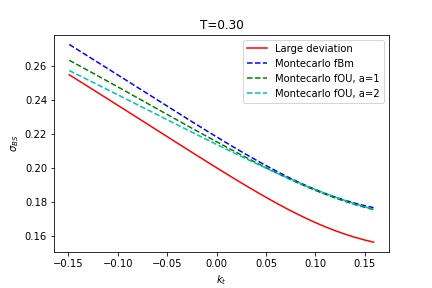
Refer to caption
Refer to caption
Refer to caption
Figure 1: Implied volatility smile with fBM-driven stochastic volatility, fOU-driven stochastic volatility with a=1𝑎1a=1, fOU-driven stochastic volatility with a=2𝑎2a=2 and large deviation approximation (4.8). Model parameters: H=0.3,ρ=0.7,σ0=0.2formulae-sequence𝐻0.3formulae-sequence𝜌0.7subscript𝜎00.2H=0.3,\rho=-0.7,\sigma_{0}=0.2 and η=1.5𝜂1.5\eta=1.5. Monte Carlo parameters: 106superscript10610^{6} trajectories and 500500500 time-steps. Recall that kt=xt1/2Hsubscript𝑘𝑡𝑥superscript𝑡12𝐻k_{t}=xt^{1/2-H}. The rate function is computed with the Ritz method with N=5𝑁5N=5 Fourier basis function.
Refer to caption
Refer to caption
Refer to caption
Refer to caption
Figure 2: Implied volatility smile with fBM-driven stochastic volatility, fOU-driven stochastic volatility with a=1𝑎1a=1, fOU-driven stochastic volatility with a=2𝑎2a=2 and large deviation approximation (4.8). Model parameters: H=0.3,ρ=0.7,σ0=0.2formulae-sequence𝐻0.3formulae-sequence𝜌0.7subscript𝜎00.2H=0.3,\,\rho=-0.7,\sigma_{0}=0.2 and η=1.5𝜂1.5\eta=1.5. Monte Carlo parameters: 106superscript10610^{6} trajectories and 500500500 time-steps. We plot each model fixing the time horizon and varying x𝑥x, where kt=xt1/2Hsubscript𝑘𝑡𝑥superscript𝑡12𝐻k_{t}=xt^{1/2-H}. Rate function is computed with the Ritz method with N=5𝑁5N=5 Fourier basis function.

We test now the moderate deviation asymptotics in Remark 4.8. In order to do so, let us recall an expansion to the fourth order of the rate function that allows us to use the second order moderate deviation.444This expansion is given in (Friz et al., 2022, Lemma 6.1), where the kernel C(ts)H1/2𝐶superscript𝑡𝑠𝐻12C(t-s)^{H-1/2} is used. However, in the proof of this result the specific shape of the kernel is not used, but only self-similarity, and therefore it holds for K(t,s)𝐾𝑡𝑠K(t,s) in (3.5) as well. We denote now KHf(t)=0tKH(t,s)f(s)𝑑ssubscript𝐾𝐻𝑓𝑡superscriptsubscript0𝑡subscript𝐾𝐻𝑡𝑠𝑓𝑠differential-d𝑠K_{H}f(t)=\int_{0}^{t}K_{H}(t,s)f(s)ds and with KH¯¯subscript𝐾𝐻\overline{K_{H}} the adjoint of KHsubscript𝐾𝐻K_{H} in L2[0,1]superscript𝐿201L^{2}[0,1], so that KH¯f(u)=u1KH(t,u)f(t)𝑑t¯subscript𝐾𝐻𝑓𝑢superscriptsubscript𝑢1subscript𝐾𝐻𝑡𝑢𝑓𝑡differential-d𝑡\overline{K_{H}}f(u)=\int_{u}^{1}K_{H}(t,u)f(t)dt, where again KHsubscript𝐾𝐻K_{H} is the fBM kernel in (3.5).

Lemma 5.1 (Fourth order energy expansion).

Let us assume that σ()𝜎\sigma(\cdot) is countinuously differentiable two times. Let J(x)𝐽𝑥J(x) be the energy function in (4.7). Then

J(x)=J′′(0)2x2+J′′′(0)3!x3+J(4)(0)4!x4+O(x5)𝐽𝑥superscript𝐽′′02superscript𝑥2superscript𝐽′′′03superscript𝑥3superscript𝐽404superscript𝑥4𝑂superscript𝑥5\begin{split}J(x)&=\frac{J^{\prime\prime}(0)}{2}x^{2}+\frac{J^{\prime\prime\prime}(0)}{3!}x^{3}+\frac{J^{(4)}(0)}{4!}x^{4}+O(x^{5})\,\\ \end{split} (5.3)

where

J′′(0)=1σ(0)2,J′′′(0)=6ρσ(0)σ(0)4KH1,1,formulae-sequencesuperscript𝐽′′01𝜎superscript02superscript𝐽′′′06𝜌superscript𝜎0𝜎superscript04subscript𝐾𝐻11J^{\prime\prime}(0)=\frac{1}{\sigma(0)^{2}},\quad J^{\prime\prime\prime}(0)=-6\frac{\rho\sigma^{\prime}(0)}{\sigma(0)^{4}}\langle K_{H}1,1\rangle,

and

J(4)(0)=12σ(0)2σ(0)6{9ρ2KH1,12ρ2(KH1)2,1(KH¯1)2,12ρ2KH1,KH¯1}+12σ′′(0)σ(0)5ρ2(KH1)2,1.\begin{split}J^{(4)}(0)&=12\frac{\sigma^{\prime}(0)^{2}}{\sigma(0)^{6}}\left\{9\rho^{2}\langle K_{H}1,1\rangle^{2}-\rho^{2}\langle(K_{H}1)^{2},1\rangle-\langle(\overline{K_{H}}1)^{2},1\rangle-2\rho^{2}\langle K_{H}1,\overline{K_{H}}1\rangle\right\}+\\ &-12\frac{\sigma^{\prime\prime}(0)}{\sigma(0)^{5}}\rho^{2}\langle(K_{H}1)^{2},1\rangle.\end{split}

Plugging (5.3) into (4.10) and fixing n=4𝑛4n=4, from straightforward computations, we obtain the equivalent asymptotic formula

σ(t,t)=ΣfOU(0)+ΣfOU(0)xtβ+ΣfOU′′(0)2x2t2β+o(t2H2β)𝜎𝑡subscript𝑡subscriptΣ𝑓𝑂𝑈0superscriptsubscriptΣ𝑓𝑂𝑈0𝑥superscript𝑡𝛽superscriptsubscriptΣ𝑓𝑂𝑈′′02superscript𝑥2superscript𝑡2𝛽𝑜superscript𝑡2𝐻2𝛽\sigma(t,\ell_{t})=\Sigma_{fOU}(0)+\Sigma_{fOU}^{\prime}(0)xt^{\beta}+\frac{\Sigma_{fOU}^{\prime\prime}(0)}{2}x^{2}t^{2\beta}+o(t^{2H-2\beta}) (5.4)

where

ΣfOU(0)=σ(0),ΣfOU(0)=ρσ(0)KH1,1σ(0),ΣfOU′′(0)2=σ(0)2σ(0)3{3ρ2KH1,12+ρ22(KH1)2,1+12(KH¯1)2,1+ρ2K1,KH¯1}+σ′′(0)σ(0)2ρ22(KH1)2,1.\begin{split}\Sigma_{fOU}(0)&=\sigma(0),\quad\Sigma_{fOU}^{\prime}(0)=\frac{\rho\sigma^{\prime}(0)\langle K_{H}1,1\rangle}{\sigma(0)},\\ \frac{\Sigma_{fOU}^{\prime\prime}(0)}{2}&=\frac{\sigma^{\prime}(0)^{2}}{\sigma(0)^{3}}\left\{-3\rho^{2}\langle K_{H}1,1\rangle^{2}+\frac{\rho^{2}}{2}\langle(K_{H}1)^{2},1\rangle+\frac{1}{2}\langle(\overline{K_{H}}1)^{2},1\rangle+\rho^{2}\langle K1,\overline{K_{H}}1\rangle\right\}\\ &+\frac{\sigma^{\prime\prime}(0)}{\sigma(0)^{2}}\frac{\rho^{2}}{2}\langle(K_{H}1)^{2},1\rangle.\end{split}

We plot in Figure 3 implied volatilities computed via Monte Carlo simulations and the corresponding approximation given in (5.4). We take again σ()𝜎\sigma(\cdot) as in(5.2), with parameters H=0.3,ρ=0.7,σ0=0.2,η=0.2formulae-sequence𝐻0.3formulae-sequence𝜌0.7formulae-sequencesubscript𝜎00.2𝜂0.2H=0.3,\rho=-0.7,\sigma_{0}=0.2,\eta=0.2, and β=0.125𝛽0.125\beta=0.125. We first note that we fix n=4𝑛4n=4 in (4.10), and so we choose β(2Hn+1,2Hn]𝛽2𝐻𝑛12𝐻𝑛\beta\in(\frac{2H}{n+1},\frac{2H}{n}], that is the interval (0.12,0.15]0.120.15(0.12,0.15]. With respect to our previous experiments, we also take the smaller vol of vol parameter η=0.2𝜂0.2\eta=0.2, which is in line with the choices in Bayer et al. (2019); Friz et al. (2022). Indeed, the quality of the approximation deteriorates as η𝜂\eta grows, and for larger η𝜂\eta the asymptotic formula (5.4) is accurate on a smaller time interval.
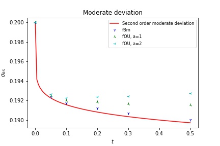
Refer to caption
Figure 3: Moderate deviation implied volatilities with fBM-driven stochastic volatility (blue), with fOU-driven stochastic volatility with a=1𝑎1a=1 (green) and fOU-driven stochastic volatility with a=2𝑎2a=2 (light blue), t=xt1/2H+βsubscript𝑡𝑥superscript𝑡12𝐻𝛽\ell_{t}=xt^{1/2-H+\beta} with x=0.3𝑥0.3x=0.3 and β=0.125𝛽0.125\beta=0.125. Model parameters: H=0.3,ρ=0.7,σ0=0.2formulae-sequence𝐻0.3formulae-sequence𝜌0.7subscript𝜎00.2H=0.3,\rho=-0.7,\sigma_{0}=0.2 and η=0.2𝜂0.2\eta=0.2. Monte Carlo parameters: 107superscript10710^{7} trajectories, 500500500 time-steps. We plot each model with fixed x𝑥x and varying maturity.

In Figure 4 we compare, with kt=xtH1/2subscript𝑘𝑡𝑥superscript𝑡𝐻12k_{t}=xt^{H-1/2}, x>0𝑥0x>0, the absolute value of the large deviations finite difference implied skew

Ψt:=|σBS(t,kt)σBS(t,kt)|2ktassignsubscriptΨ𝑡subscript𝜎𝐵𝑆𝑡subscript𝑘𝑡subscript𝜎𝐵𝑆𝑡subscript𝑘𝑡2subscript𝑘𝑡\Psi_{t}:=\frac{|\sigma_{BS}(t,k_{t})-\sigma_{BS}(t,-k_{t})|}{2k_{t}} (5.5)

computed on fBm-driven and fOU-driven stochastic volatility models, with the asymptotic skew expected from Corollary 4.7, where we also use the approximation, as x0𝑥0x\to 0,

ΣfOU(x)ΣfOU(x)2xΣfOU(0)=ρσ(0)KH1,1σ(0).similar-tosubscriptΣ𝑓𝑂𝑈𝑥subscriptΣ𝑓𝑂𝑈𝑥2𝑥superscriptsubscriptΣ𝑓𝑂𝑈0𝜌superscript𝜎0subscript𝐾𝐻11𝜎0\frac{\Sigma_{fOU}(x)-\Sigma_{fOU}(-x)}{2x}\sim\Sigma_{fOU}^{\prime}(0)=\frac{\rho\sigma^{\prime}(0)\langle K_{H}1,1\rangle}{\sigma(0)}.

We observe that, consistently with the smile slopes observed in Figure 2, larger mean-reversion parameters a𝑎a correspond to flatter smiles and smaller skews (in absolute value), smaller mean-reversion parameters a𝑎a correspond to steeper smiles and larger skews (in absolute value), fBm has a larger skew than fOU, and the asymptotic skew is even larger than the one generated from fBm, although very close to it. As maturity t0𝑡0t\to 0, the difference between all these skews vanishes.

This could reflect the fact that larger mean-reversion parameters a𝑎a give more concentrated volatility trajectories, with V𝑉V in (5.1) staying closer to 00 and therefore the stochastic volatility path (σ0exp(η2Vt))t>0subscriptsubscript𝜎0𝜂2subscript𝑉𝑡𝑡0(\sigma_{0}\exp(\frac{\eta}{2}\,V_{t}))_{t>0} staying closer to the spot-vol σ0subscript𝜎0\sigma_{0}. This may produce flatter implied volatility surfaces and explain smiles and skews observed in Figures 2, 3 and 4 corresponding to larger a𝑎a’s. On the short end of the surface, however, all of these have to coincide due to our asymptotic results. Let us also mention that the discrepancy observed in Figure 2 on the level of the smile (regardless of the skew), between the asymptotic red line and all the simulated “positive maturity” lines is likely due to a term-structure term of order t2Hsuperscript𝑡2𝐻t^{2H}, for which we refer the reader to Friz et al. (2022) (large deviations setting) and El Euch et al. (2019) (central limit setting).
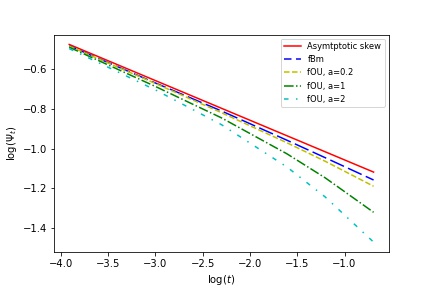
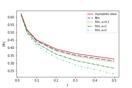
Refer to caption
Refer to caption
Figure 4: Implied skew in (5.5) with fBm-driven stochastic volatility, fOU-driven stochastic volatility with a=0.2𝑎0.2a=0.2, a=1𝑎1a=1, a=2𝑎2a=2 and asymptotic skew from (4.9). Model parameters: H=0.3,ρ=0.7,σ0=0.2formulae-sequence𝐻0.3formulae-sequence𝜌0.7subscript𝜎00.2H=0.3,\rho=-0.7,\sigma_{0}=0.2 and η=1.5𝜂1.5\eta=1.5. Monte Carlo parameters: 107superscript10710^{7} trajectories and 500500500 time-steps. We take x=0.01𝑥0.01x=0.01 (recall that kt=xt1/2Hsubscript𝑘𝑡𝑥superscript𝑡12𝐻k_{t}=xt^{1/2-H}). Log-plot on the left hand side, linear plot on the right hand side.

6 Conclusion

In this paper, we prove a short-time large deviation principle for stochastic volatility models, with volatility given as a function of a Volterra process. This result holds without strict self-similarity assumptions on the processes driving the model, and can therefore be applied to some notable examples of (non self-similar) rough volatility models.

We first consider an application to the log-modulated rough stochastic volatility models introduced in Bayer et al. (2021). We derive short-maturity asymptotics for European option prices and implied volatility surfaces. Our results on the implied skew at the large deviations regime are consistent with the results at the Edgeworth central-limit regime derived in Bayer et al. (2021), but allow for valuation of options further from the money.

Then we consider models where volatility is given as a function of a fractional Ornstein-Uhlenbeck process, as e.g. in the seminal work Gatheral et al. (2018). In this case we find that the limit short maturity behavior of option prices and implied volatilities, as well as the short time implied skew, is the same as the one of a model driven by a fractional Brownian motion. We investigate this fact numerically on simulation results, discussing also moderate deviations pricing and implied skew asymptotics.

Appendix A The large deviations principle

Large deviations give an asymptotic computation of small probabilities on an exponential scale (see e.g. Dembo and Zeitouni (1998) as a reference on this topic). We recall some basic definitions (see e.g. Section 1.2 in Dembo and Zeitouni (1998)). Throughout this paper a speed function is a sequence {vn:n1}conditional-setsubscript𝑣𝑛𝑛1\{v_{n}:n\geq 1\} such that limnvn=subscript𝑛subscript𝑣𝑛\lim_{n\to\infty}v_{n}=\infty. A sequence of random variables {Zn:n1}conditional-setsubscript𝑍𝑛𝑛1\{Z_{n}:n\geq 1\}, taking values on a topological space 𝒳𝒳\mathcal{X}, satisfies the large deviation principle (LDP) with rate function I𝐼I and speed function vnsubscript𝑣𝑛v_{n} if I:𝒳[0,]:𝐼𝒳0I:\mathcal{X}\to[0,\infty] is a lower semicontinuous function,

lim infn1vnlogP(ZnO)infxOI(x)subscriptlimit-infimum𝑛1subscript𝑣𝑛𝑃subscript𝑍𝑛𝑂subscriptinfimum𝑥𝑂𝐼𝑥\liminf_{n\to\infty}\frac{1}{v_{n}}\log P(Z_{n}\in O)\geq-\inf_{x\in O}I(x)

for all open sets O𝑂O, and

lim supn1vnlogP(ZnC)infxCI(x)subscriptlimit-supremum𝑛1subscript𝑣𝑛𝑃subscript𝑍𝑛𝐶subscriptinfimum𝑥𝐶𝐼𝑥\limsup_{n\to\infty}\frac{1}{v_{n}}\log P(Z_{n}\in C)\leq-\inf_{x\in C}I(x)

for all closed sets C𝐶C. A rate function is said to be good if all its level sets {{z𝒵:I(z)η}:η0}conditional-setconditional-set𝑧𝒵𝐼𝑧𝜂𝜂0\{\{z\in\mathcal{Z}:I(z)\leq\eta\}:\eta\geq 0\} are compact. Therefore, if an LDP holds, and ΓΓ\Gamma is a Borel set such that infxΓoI(x)=infxΓ¯I(x)subscriptinfimum𝑥superscriptΓ𝑜𝐼𝑥subscriptinfimum𝑥¯Γ𝐼𝑥\inf_{x\in\Gamma^{o}}I(x)=\inf_{x\in\bar{\Gamma}}I(x) (ΓosuperscriptΓ𝑜\Gamma^{o} and Γ¯¯Γ\bar{\Gamma} are the interior and the closure of ΓΓ\Gamma respectively), then

limn1vnlogP(ZnΓ)=I(Γ)subscript𝑛1subscript𝑣𝑛𝑃subscript𝑍𝑛Γ𝐼Γ\lim_{n\to\infty}\frac{1}{v_{n}}\log P(Z_{n}\in\Gamma)=-I(\Gamma)

where I(Γ)=infxΓoI(x)=infxΓ¯I(x).𝐼Γsubscriptinfimum𝑥superscriptΓ𝑜𝐼𝑥subscriptinfimum𝑥¯Γ𝐼𝑥I(\Gamma)=\displaystyle\inf_{x\in\Gamma^{o}}I(x)=\inf_{x\in\bar{\Gamma}}I(x). In this case we write

P(ZnΓ)eI(Γ)vn.𝑃subscript𝑍𝑛Γsuperscript𝑒𝐼Γsubscript𝑣𝑛P(Z_{n}\in\Gamma)\approx e^{-{I(\Gamma)}{v_{n}}}.

Moreover {Zn:n1}conditional-setsubscript𝑍𝑛𝑛1\{Z_{n}:n\geq 1\} is exponentially tight with respect to the speed function vnsubscript𝑣𝑛v_{n} if, for all b>0𝑏0b>0, there exists a compact Kb𝒳subscript𝐾𝑏𝒳K_{b}\subset\mathcal{X} such that

lim supn1vnlogP(ZnKb)b.subscriptlimit-supremum𝑛1subscript𝑣𝑛𝑃subscript𝑍𝑛subscript𝐾𝑏𝑏\limsup_{n\to\infty}\frac{1}{v_{n}}\log P(Z_{n}\notin K_{b})\leq-b.

The concept of exponential tightness plays a crucial role in large deviations; in fact this condition is often required to establish that the LDP holds for a sequence of random variables taking values on an infinite dimensional topological space. In this paper we refer to condition (8) and (9) in Section 2 in Macci and Pacchiarotti (2017)) which yield the exponential tightness when the topological space 𝒳𝒳\mathcal{X} of the continuous function is equipped with the topology of the uniform convergence.

References

  • Ait-Sahalia et al. (2020) Y. Ait-Sahalia, C. Li, and C.X. Li (2020) Implied stochastic volatility models. The Review of Financial Studies, 34:394–450.
  • Alòs and Leon (2017) E. Alòs and J. A. León (2017) On the curvature of the smile in stochastic volatility models. SIAM Journal on Financial Mathematics, 8(1):373-399.
  • Alòs et al. (2007) E. Alòs, J. A. León and J. Vives (2007) On the short-time behavior of the implied volatility for jump-diffusion models with stochastic volatility. Finance and Stochastics, 11(4):571–589.
  • Atkinson (2008) K.E. Atkinson (2008) An introduction to numerical analysis, 2nd ed, Wiley India Pvt. Limited
  • Baldi and Pacchiarotti (2022) P. Baldi and B. Pacchiarotti (2022) Large Deviations of continuous Gaussian processes: from small noise to small time. Preprint arXiv:2207.12037.
  • Bayer et al. (2020) C. Bayer, P. K. Friz, P. Gassiat, J. Martin and B. Stemper (2020) A regularity structure for rough volatility. Mathematical Finance, 30(3):782–832.
  • Bayer et al. (2016) C. Bayer, P. K. Friz and J. Gatheral (2016) Pricing under rough volatility. Quantitative Finance, 16(6):887–904.
  • Bayer et al. (2019) C. Bayer, P. K. Friz, A. Gulisashvili, B. Horvath and B. Stemper (2019) Short-time near-the-money skew in rough fractional volatility models. Quantitative Finance, 19(5):779–798.
  • Bayer et al. (2021) C. Bayer, F. Harang and P. Pigato (2021) Log-modulated rough stochastic volatility models. SIAM Journal on Financial Mathematics, 12(3):1257–1284.
  • Bourgey et al. (2023) F. Bourgey, S. De Marco, P. K. Friz and P. Pigato (2023) Local volatility under rough volatility. Mathematical Finance, 33(4):1119-1145
  • Catalini and Pacchiarotti (2023) G. Catalini and B. Pacchiarotti (2023) Asymptotics for multifactor Volterra type stochastic volatility models. Stochastic Analysis and Applications, 41(6):1025-1055.
  • Cellupica and Pacchiarotti (2021) M. Cellupica and B. Pacchiarotti (2021) Pathwise Asymptotics for Volterra Type Stochastic Volatility Models. Journal of Theoretical Probability, 34(2):682–727.
  • Cheridito et al. (2003) P. Cheridito, H. Kawaguchi and M. Maejima (2003) Fractional Ornstein-Uhlenbeck processes. Electronic Journal of Probability, 8:1–14.
  • Dembo and Zeitouni (1998) A. Dembo and O. Zeitouni (1998) Large Deviations Techniques and Applications, Jones and Bartlett, Boston MA.
  • El Euch et al. (2019) O. El Euch, M. Fukasawa, J. Gatheral and M. Rosenbaum (2019) Short-term at-the-money asymptotics under stochastic volatility models. SIAM Journal on Financial Mathematics, 10(2):491–511.
  • Forde et al. (2020) M. Forde, M. Fukasawa, S. Gerhold and B. Smith (2022) The Riemann-Liouville field and its GMC as H0𝐻0H\to 0, and skew flattening for the rough Bergomi model. Statistics and Probability Letters, 181:10926.
  • Forde et al. (2021) M. Forde, S. Gerhold and B. Smith (2021) Small-time, large-time and H0𝐻0H\to 0 asymptotics for the rough Heston model. Mathematical Finance, 31:203–241.
  • Forde and Zhang (2017) M. Forde and H. Zhang (2017) Asymptotics for rough stochastic volatility models. SIAM Journal on Financial Mathematics, 8(1):114–145.
  • Friz et al. (2021) P.K. Friz, P. Gassiat and P. Pigato (2021) Precise asymptotics: Robust stochastic volatility models. Annals of Applied Probability, 31(2):896–940.
  • Friz et al. (2022) P.K. Friz, P. Gassiat and P. Pigato (2022) Short dated smile under Rough Volatility: asymptotics and numerics. Quantitative Finance, 22(3):463–480.
  • Friz et al. (2021) P.K. Friz, P. Pigato and J. Seibel (2021) The Step Stochastic Volatility Model. Risk magazine, June 2021, (Longer version available at at SSRN: https://ssrn.com/abstract=3595408).
  • Fukasawa (2011) M. Fukasawa (2011) Asymptotic analysis for stochastic volatility: Martingale expansion. Finance and Stochastics, 15:635–654.
  • Fukasawa (2017) M. Fukasawa (2017) Short-time at-the-money skew and rough fractional volatility. Quantitative Finance, 17(2):189–198.
  • Fukasawa (2020) M. Fukasawa (2020) Volatility has to be rough. Quantitative Finance, 21(1):1–8.
  • Gao and Lee (2014) K. Gao and R. Lee. (2014) Asymptotics of implied volatility to arbitrary order. Finance and Stochastics, 18:349–392.
  • Garnier and Sølna (2017) J. Garnier and K. Sølna (2017) Correction to Black-Scholes Formula Due to Fractional Stochastic Volatility. SIAM Journal on Financial Mathematics, 8:560–588.
  • Garnier and Sølna (2018a) J. Garnier and K. Sølna (2018a) Option pricing under fast-varying and rough stochastic volatility. Annals of Finance, 14:489–516.
  • Garnier and Sølna (2019) J. Garnier and K. Sølna (2019) Option pricing under fast-varying long-memory stochastic volatility. Mathematical Finance, 29:39–83.
  • Garnier and Sølna (2020a) J. Garnier and K. Sølna (2020a) Implied Volatility Structure in Turbulent and Long-Memory Markets. Frontiers in Applied Mathematics and Statistics , 29 April 2020.
  • Garnier and Sølna (2020b) J. Garnier and K. Sølna (2020b) Optimal hedging under fast-varying stochastic volatility. SIAM Journal on Financial Mathematics, 11(1):274–325
  • Gassiat (2019) P. Gassiat (2019) On the martingale property in the Rough Bergomi model. Electronic Communications in Probability, 24:1–9
  • Gatheral et al. (2018) J. Gatheral, T.Jaisson and M. Rosenbaum (2018) Volatility is rough. Quantitative Finance, 18(6):933–949.
  • Gelfand and Fomin (1963) I.M. Gelfand and S.V. Fomin (1963) Calculus of variations. Revised English edition translated and edited by Richard A. Silverman Prentice-Hall.
  • Gulisashvili (2018) A. Gulisashvili (2018) Large Deviation Principle for Volterra type Fractional Stochastic Volatility Models. SIAM Journal on Financial Mathematics, 9(3):1102–1136.
  • Gulisashvili (2020) A. Gulisashvili (2020) Gaussian stochastic volatility models: scaling regimes, large deviations, and moment explosions. Stochastic Processes and their Applications, 130(6):3648–3686.
  • Gulisashvili (2021) A. Gulisashvili (2021) Time-inhomogeneous Gaussian stochastic volatility models: Large deviations and super roughness. Stochastic Processes and their Applications, 139:37–79.
  • Gulisashvili (2022) A. Gulisashvili (2022) Multivariate Stochastic Volatility Models and Large Deviation Principles. Preprint arXiv:2203.09015.
  • Gulisashvili et al. (2018a) A. Gulisashvili, F. Viens and X. Zhang (2018a) Small-Time Asymptotics for Gaussian Self-Similar Stochastic Volatility Models, Applied Mathematics & Optimization, 1–41.
  • Gulisashvili et al. (2018b) A. Gulisashvili, F. Viens and X. Zhang (2018b) Extreme-strike asymptotics for general Gaussian stochastic volatility models. Annals of Finance, 15(1):59–101.
  • Guyon (2021) J. Guyon (2021) Dispersion-Constrained Martingale Schrödinger Problems and the Exact Joint S&P 500/VIX Smile Calibration Puzzle. Available at SSRN: https://ssrn.com/abstract=3853237 or http://dx.doi.org/10.2139/ssrn.3853237
  • El Amrani and Guyon (2023) M. El Amrani and J. Guyon (2023) Does the term-structure of equity at-the-money skew really follow a power law? Risk magazine, July 2023, (Longer version available at at SSRN: https://ssrn.com/abstract=4174538).
  • Fouque and Hu (2018) J.P. Fouque and R. Hu (2018) Optimal Portfolio under Fast Mean-Reverting Fractional Stochastic Environment SIAM Journal of Financial Mathematics, 9(2):564-601.
  • Hager and Neuman (2021) P. Hager and E. Neuman (2021) The Multiplicative Chaos of H=0𝐻0H=0 Fractional Brownian Fields. Annals of applied probability, 32(3) 2139–2179.
  • Horvath et al. (2019) B. Horvath, A. Jacquier and C. Lacombe (2019) Asymptotic behaviour of randomised fractional volatility models. Journal of Applied Probability, 56(2):496–523.
  • Jacquier et al. (2018) A. Jacquier, M.S. Pakkanen and H. Stone (2018) Pathwise large deviations for the rough Bergomi model. Journal of Applied Probability, 55(4):1078–1092.
  • Jacquier and Pannier (2022) A. Jacquier and A. Pannier (2022) Large and moderate deviations for stochastic Volterra systems, Stochastic Processes and their Applications, 149:142–187.
  • Jourdain (2004) B. Jourdain (2004) Loss of martingality in asset price models with lognormal stochastic volatility, preprint Cermics, 267:2004.
  • Lee (2005) R. W. Lee (2005) Implied volatility: Statics, dynamics, and probabilistic interpretation, in Recent Advances in Applied Probability, Springer, New York, 241-268.
  • Lions and Musiela (2007) P. L. Lions and M. Musiela (2007) Correlations and bounds for stochastic volatility models, In Annales de l’Institut Henri Poincare (C) Non Linear Analysis, 24:1–16.
  • Macci and Pacchiarotti (2017) C. Macci and B. Pacchiarotti (2017) Exponential tightness for Gaussian processes with applications to some sequences of weighted means. Stochastics 89(2):469–484.
  • Medvedev and Scaillet (2003) A. Medvedev and O. Scaillet (2003) A simple calibration procedure of stochastic volatility models with jumps by short term asymptotics. Research Paper No. 93, September 2003, FAME International Center for Financial Asset Management and Engineering. Available at SSRN 477441, 2003.
  • Medvedev and Scaillet (2007) A., Medvedev and O. Scaillet (2007) Approximation and calibration of short-term implied volatilities under jump-diffusion stochastic volatility. The Review of Financial Studies, 20(2):427–459.
  • Neuman and Rosenbaum (2018) E. Neuman and M. Rosenbaum (2018) Fractional Brownian motion with zero Hurst parameter: a rough volatility viewpoint. Electronic Communications in Probability, 23(61):1–12.
  • Nualart (2006) D. Nualart (2006) Malliavin Calculus and Related Topics, Springer, Berlin.
  • Osajima (2015) Y. Osajima (2015) General asymptotics of Wiener functionals and application to implied volatilities. In Large Deviations and Asymptotic Methods in Finance, 137–173, Springer.
  • Pigato (2019) P. Pigato (2019) Extreme at-the-money skew in a local volatility model. Finance and Stochastics, 23:827–859.
  • Press et al. (2012) W. H. Press, S. A. Teukolsky, W. T. Vetterling and B. P. Flannery (2007) Numerical Recipes: The Art of Scientific Computing (3rd ed.). New York: Cambridge University Press.
  • Sin (1998) C. A. Sin (1998) Complications with stochastic volatility models. Advances in Applied Probability, 30(1):256–268.