A subgradient method with non-monotone line search

Abstract

In this paper we present a subgradient method with non-monotone line search for the minimization of convex functions with simple convex constraints. Different from the standard subgradient method with prefixed step sizes, the new method selects the step sizes in an adaptive way. Under mild conditions asymptotic convergence results and iteration-complexity bounds are obtained. Preliminary numerical results illustrate the relative efficiency of the proposed method.

1 Introduction

The subgradient method for solving non-differentiable convex optimization problems has its origin in the 60’s, see [5, 23]. Over the years it has been the subject of much interest, attracting the attention of the scientific community working on convex optimization. One of the factors that explains the interest in the subgradient method lies in its simplicity and ease of implementation for a wide range of problems, where the sub-differential of the objective function can be easily computed. In addition, this method has low storage cost and ready exploitation of separability and sparsity, which makes it attractive in solving large-scale problems. For all these reasons, several variants of this method have emerged and properties of it have been discovered throughout the years, resulting in a wide literature on the subject; including for exemple [2, 6, 13, 14, 18, 19, 20, 21] and the references therein.

The classical subgradient method employs a predefined sequence of step sizes. Standard choices include a constant step size and also sequences that converge to zero sublinearly. In this paper, we propose a subgradient method with adaptive step sizes for the minimization of convex functions with simple convex constraints in which a projection on it is easily computed. At each iteration, the selection of the step size is done by a line search in the direction opposite to the subgradient. Since, in general, this direction is not a descent direction, we endow the method with a non-monotone line search. The possible increase in the objective function values at consecutive iterations is limited by a sequence of positive parameters that implicitly controls the step sizes. Remarkably, it is shown that the proposed method enjoys convergence and complexity properties similar to the ones of the classical subgradient method when the sequence that controls the non-monotonicity satisfies suitable conditions. Illustrative numerical results are also presented. They show that the proposed non-monotone method compares favorably with the classical subgradient method endowed with usual prefixed step sizes.

The organization of the paper is as follows. In Section 2, we present some notation and basic results used in our presentation. In Section 3 we describe the subgradient method with non-monotone line search and the main results of the present paper, including the converge theorems and iteration-complexity bounds. Some numerical experiments are provided in Section 4. We conclude the paper with some remarks in Section 5.

2 Preliminaries

In this section we present some notations, definitions, and results that will be used throughout the paper, which can be found in [1, 11].

Denotes ${\mathbb{N}}:=\{1,2,3,\ldots\}$. A function $f\colon\mathbb{R}^{n}\to\mathbb{R}$ is said to be $\sigma$-strongly convex with modulus $\sigma\geq 0$ if $f(\tau x+(1-\tau)y)\leq\tau f(x)+(1-\tau)f(y)-\frac{\sigma}{2}\tau(1-\tau)\|x-y\|^{2}$, for all $x,y\in{\mathbb{R}^{n}}$ and $\tau\in[0,1]$. For $\sigma=0$ we say that $f$ is a convex function.

Proposition 2.1.

The function $f:\mathbb{R}^{n}\to\mathbb{R}$ is $\sigma$-strongly convex with modulus $\sigma\geq 0$ if and only if $f(y)\geq f(x)+\langle v,y-x\rangle+({\sigma}/{2})\|y-x\|^{2}$, for all $x,y\in\mathbb{R}^{n}$ and all $v\in\partial f(x)$.

A function $f:\mathbb{R}^{n}\to\mathbb{R}$ is $L_{f,{\cal C}}$-Lipschitz continuous on ${\cal C}\subset\mathbb{R}^{n}$ if there exist a constant $L_{f,{\cal C}}>0$ such that $|f(x)-f(y)|\leq L_{f,{\cal C}}\|x-y\|$, for all $x,y\in{\cal C}$. Whenever $C=\mathbb{R}^{n}$ we set $L_{f}\equiv L_{f,\mathbb{R}^{n}}$.

Proposition 2.2.

Let $f:\mathbb{R}^{n}\to\mathbb{R}$ be a convex. Then, for all $x\in\mathbb{R}^{n}$ the set $\partial f(x)$ is a non-empty, convex, compact subset of $\mathbb{R}^{n}$. In addition, $f$ is $L_{f,{\cal C}}$-Lipschitz function on ${\cal C}\subset\mathbb{R}^{n}$ if and only if $\|v\|\leq L_{f,{\cal C}}$ for all $v\in\partial f(x)$ and $x\in{\cal C}$.

Remark 2.3.

In view of Proposition 2.2, if ${\cal C}\subset\mathbb{R}^{n}$ is a compact set then $f$ is a $L_{f,\cal C}$-Lipschitz function on ${\cal C}\subset\mathbb{R}^{n}$ for some $L_{f,\cal C}>0$.

Definition 2.4.

Let ${\cal C}\subset{\mathbb{R}}^{n}$ be a closed convex set. The projection map, denoted by ${\cal P}_{\cal C}:{\mathbb{R}}^{n}\rightrightarrows{\cal C}$, is defined as follows ${\cal P}_{\cal C}(y):=\arg\min\{\|y-z\|:~{}z\in{\cal C}\}.$

The next lemma presents an important property of the projection.

Proposition 2.5.

Let $y\in{\mathbb{R}}^{n}$ and $z\in{\cal C}$. Then, we have $\left\|{\cal P}_{\cal C}(y)-z\right\|^{2}\leq\|y-z\|^{2}.$

Definition 2.6.

Let $S$ be a nonempty subset of $\mathbb{R}^{n}$. A sequence $(v^{k})_{k\in\mathbb{N}}\subset\mathbb{R}^{n}$ is said to be quasi-Fejér convergent to $S$, if and only if, for all $v\in S$ there exists ${\bar{k}}\geq 0$ and a summable sequence $(\epsilon_{k})_{k\in\mathbb{N}}$, such that $\|v^{k+1}-v\|^{2}\leq\|v^{k}-v\|^{2}+\epsilon_{k}$ for all $k\geq{\bar{k}}$.

In the following lemma, we state the main properties of quasi-Fejér sequences that we will need; a comprehensive study on this topic can be found in [4].

Lemma 2.7.

Let $(v^{k})_{k\in\mathbb{N}}$ be quasi-Fejér convergent to $S$. Then, the following conditions hold:

• the sequence $(v^{k})_{k\in\mathbb{N}}$ is bounded;

• if a cluster point ${\bar{v}}$ of $(v^{k})_{k\in\mathbb{N}}$ belongs to $S$, then $(v^{k})_{k\in\mathbb{N}}$ converges to ${\bar{v}}$.

3 Subgradient method with non-monotone line search

We are interested in the following constrained optimization problem

$$\begin{array}[]{c}\min f(x)\\ \mbox{s.t. }x\in{\cal C},\end{array}$$ (1)

where $f:\mathbb{R}^{n}\to\mathbb{R}$ is a convex function and ${\cal C}\subset\mathbb{R}^{n}$ is a closed and convex set. Denote by $\Omega^{*}$ the optimal set of the problem (1) and by $f^{*}$ the optimal value. Throughout the paper we will consider problem (1) under the following two assumptions:

1. $f:\mathbb{R}^{n}\to\mathbb{R}$ is a convex function and $L_{f,{\cal C}}$-Lipschitz continuous;

2. $f^{*}:=\inf_{x\in{\cal C}}f(x)>-\infty.$

We propose the following conceptual algorithm to find a solution of problem (1).

SubGrad projection method with non-monotone line search Step 0. Fix $c>0$, $(\gamma^{k})_{k\in\mathbb{N}}\subset\mathbb{R}_{++}$ a non-increasing sequence, $\rho,\beta\in(0,1)$ and $\alpha>0$. Choose an initial point $x_{1}\in C$. Set $\alpha_{1}=\alpha$ and $k=1$; Step 1. Choose $s_{k}\in\partial f(x_{k})$. If $s_{k}=0$, then STOP and returns $x_{k}$; Step 2. Compute $$\ell_{k}:=\min\left\{\ell\in{\mathbb{N}}:~{}\beta^{\ell}\alpha_{k}\leq c\beta\gamma_{k},~{}f({\cal P}_{\cal C}(x_{k}-\beta^{\ell}\alpha_{k}s_{k}))\leq f(x_{k})-{\rho}\big{(}\beta^{\ell}{\alpha_{k}}\big{)}\|s_{k}\|^{2}+\gamma_{k}\right\};$$ (2) Step 3. Set $x_{k+1}:={\cal P}_{\cal C}(x_{k}-\beta^{\ell_{k}}\alpha_{k}s_{k})$, $\alpha_{k+1}:=\beta^{\ell_{k}-1}\alpha_{k}$. Update $k\leftarrow k+1$ and go to Step 1.

Remark 3.1.

It follows from [12, Theorem 4.2.3] that the set where convex functions fail to be differentiable is of zero measure. Consequently, almost every opposite direction of a subgradient is a descent direction. Therefore, we expect Algorithm 3 to be able to skip non-differentiability points that are not minimum points and then behave similarly to the gradient method with non-monotonic line search at differentiability points. It is worth to noting that the idea of using general non-monotone line searches in differentiable optimization, generalizing the non-monotone searches proposed in [10, 24], have appeared in [9, 22]. A modified version of the subgradient method with the non-monotone line search proposed in [10] was considered in [15, 16, 17].

In the following lemmas we establish general inequalities that are important in our analysis. We begin presenting the well definition of $\ell_{k}$ defined in Step 2 of Algorithm 3 and two inequalities that follows as a consequence.

Lemma 3.2.

There exists $\ell_{k}$ satisfying (2). As a consequence, the following inequalities hold:

$$\alpha_{k+1}\leq c\gamma_{k},\qquad f(x_{k+1})\leq f(x_{k})-{\rho}\beta\alpha_{k+1}\|s_{k}\|^{2}+\gamma_{k},\quad\forall k\in\mathbb{N},$$ (3)

and $x_{k+1}\in{\cal C}$, for all $k\in\mathbb{N}$.

Proof.

Since $f$ and the projection ${\cal P}_{\cal C}$ are continuous functions and the point $x_{k}\in{\cal C}$, we have $\lim_{\alpha\to 0^{+}}(f({\cal P}_{\cal C}(x_{k}-\alpha s_{k}))-f(x_{k})+\rho\alpha\|s_{k}\|^{2})=0$. Hence, due to $\gamma_{k}>0$, there exists $\eta_{k}>0$ such that $f({\cal P}_{\cal C}(x_{k}-\alpha s_{k}))-f(x_{k})+\rho\alpha\|s_{k}\|^{2}<\gamma_{k}$, for all $\alpha\in(0,{\eta_{k}}]$, or equivalently,

$$f({\cal P}_{\cal C}(x_{k}-\alpha s_{k}))\leq f(x_{k})-\rho\alpha\|s_{k}\|^{2}+\gamma_{k},\qquad\alpha\in(0,\eta_{k}].$$ (4)

Hence, due to $\beta\in(0,1)$ we have $\lim_{\ell\to 0^{+}}\beta^{\ell}{\alpha_{k}}=0$, and since $\eta_{k}>0$, we obtain that there exists ${\ell_{*}}\in{\mathbb{N}}$ such that $\ell\geq{\ell_{*}}$ implies $\beta^{\ell}{\alpha_{k}}\in(0,\eta_{k}]$. Therefore, due to (4) be hold for all $\alpha\in(0,\eta_{k}]$, there exists $\ell_{k}$ satisfying (2), which proves the first statement. The inequalities in (3) and inclusion $x_{k+1}\in{\cal C}$ follow from the definitions of $x_{k+1}$ and $\alpha_{k+1}$ in Step 3. ∎

From now on $(x_{k})_{k\in\mathbb{N}}$ denotes the sequence generated by Algorithm 3. In the next lemma we recall a classical inequality used in the study of subgradient methods. We give the proof here for the sake of completeness.

Lemma 3.3.

For any $x\in\mathbb{R}^{n}$ there holds

$$2\beta\alpha_{k+1}(f(x_{k})-f(x))\leq\|x_{k}-x\|^{2}-\|x_{k+1}-x\|^{2}+\beta^{2}\alpha_{k+1}^{2}\|s_{k}\|^{2},\quad\forall k\in\mathbb{N}.$$ (5)

In addition, if $f$ is a $\sigma$-strongly convex function then there holds

$$2\beta\alpha_{k+1}(f(x_{k})-f(x))\leq(1-\sigma\beta\alpha_{k+1})\|x_{k}-x\|^{2}-\|x_{k+1}-x\|^{2}+\beta^{2}\alpha_{k+1}^{2}\|s_{k}\|^{2},\quad\forall k\in\mathbb{N}.$$ (6)

Proof.

Since the inequality (6) becomes (5) for $\sigma=0$, it is sufficient to prove (6). It follows from the definition of $x_{k+1}$ in Step 3 of Algorithm 3, Proposition 2.5 and also definitions of $\alpha_{k+1}$ that

$$\|x_{k+1}-x\|^{2} =\|{\cal P}_{\cal C}(x_{k}-\beta^{\ell_{k}}\alpha_{k}s_{k})-x\|^{2}$$

$$\leq\|x_{k}-\beta^{\ell_{k}}\alpha_{k}s_{k}-x\|^{2}.$$ (7)

$$=\|x_{k}-x\|^{2}+2\beta\alpha_{k+1}\langle s_{k},x-x_{k}\rangle+\beta^{2}\alpha_{k+1}^{2}\|s_{k}\|^{2}.$$

Therefore, considering that $f$ is a $\sigma$-strongly convex function, it follows from Proposition 2.1 that $\langle s_{k},x-x_{k}\rangle\leq f(x)-f(x_{k})-(\sigma/2)\|x_{k}-x\|^{2}$, which substituting into (7) yields (6). The inequality (5) follows from (6) by letting $\sigma=0$. ∎

Next we present an important relationship between $(\alpha_{k})_{k\in\mathbb{N}}$ and $(\gamma_{k})_{k\in\mathbb{N}}$.

Lemma 3.4.

The following inequality holds:

$$\alpha_{k}\geq\min\left\{\alpha_{1},\frac{\gamma_{k}}{(1+\rho)L_{f,{\cal C}}^{2}}\right\},\quad\forall k\in\mathbb{N}.$$ (8)

Proof.

The inequality (8) immediately holds for $k=1$. Suppose by an absurd that there exists $k\in\mathbb{N}$ such that

$$\alpha_{k+1}<\min\left\{\alpha_{1},\frac{\gamma_{k+1}}{(1+\rho)L_{f,{\cal C}}^{2}}\right\}.$$ (9)

Since we are supposing that $(\gamma^{k})_{k\in\mathbb{N}}$ is a non-increasing sequence, using the definition of $\alpha_{k+1}$ in Step 3 of Algorithm 3 together with (9), we conclude that

$$\beta^{\ell_{k}-1}\alpha_{k}=\alpha_{k+1}<\min\Big{\{}\alpha_{1},\frac{\gamma_{k+1}}{(1+\rho)L_{f,{\cal C}}^{2}}\Big{\}}\leq\min\Big{\{}\alpha_{1},\frac{\gamma_{k}}{(1+\rho)L_{f,{\cal C}}^{2}}\Big{\}}\leq\frac{\gamma_{k}}{(1+\rho)L_{f,{\cal C}}^{2}}.$$ (10)

Considering that $f$ is $L_{f,{\cal C}}$-Lipschitz continuous and $x_{k}\in{\cal C}$, using Proposition 2.5 we have

$$f\big{(}{\cal P}_{\cal C}(x_{k}-\beta^{\ell_{k}-1}\alpha_{k}s_{k})\big{)}-f(x_{k}) \leq L_{f,{\cal C}}\|{\cal P}_{\cal C}(x_{k}-\beta^{\ell_{k}-1}\alpha_{k}s_{k})-x_{k}\|$$

$$\leq L_{f,{\cal C}}\|x_{k}-\beta^{\ell_{k}-1}\alpha_{k}s_{k}-x_{k}\|$$

$$=L_{f,{\cal C}}\beta^{\ell_{k}-1}\alpha_{k}\|s_{k}\|.$$

Using again that $L_{f,{\cal C}}$-Lipschitz continuous, it follows from Proposition 2.2 that $\|s_{k}\|\leq L_{f,{\cal C}}$. Thus, after some algebraic manipulations, the two previous inequalities imply that

$$f\big{(}{\cal P}_{\cal C}(x_{k}-\beta^{\ell_{k}-1}\alpha_{k}s_{k})\big{)}-f(x_{k})+\rho\beta^{\ell_{k}-1}\alpha_{k}\|s_{k}\|^{2} \leq L_{f,{\cal C}}\beta^{\ell_{k}-1}\alpha_{k}\|s_{k}\|+\rho\beta^{\ell_{k}-1}\alpha_{k}\|s_{k}\|^{2}$$

$$\leq\ \beta^{\ell_{k}-1}\alpha_{k}(1+\rho)L_{f,{\cal C}}^{2}.$$

Hence, using (10) we obtain that $f({\cal P}_{\cal C}(x_{k}-\beta^{\ell_{k}-1}\alpha_{k}s_{k}))-f(x_{k})+\rho\beta^{\ell_{k}-1}\alpha_{k}\|s_{k}\|^{2}<\gamma_{k}$, or equivalently

$$f\big{(}{\cal P}_{\cal C}(x_{k}-\beta^{\ell_{k}-1}\alpha_{k}s_{k})\big{)}<f(x_{k})-\rho\beta^{\ell_{k}-1}\alpha_{k}\|s_{k}\|^{2}+\gamma_{k},$$

which contradicts the definition of $\ell_{k}$ in (2). Thus, (8) holds for all $k$ and the proof is complete. ∎

In the following we combine the inequalities (3) in Lemma 3.2 with those in Lemmas 3.3 and 3.4 to provide an inequality that will allow us to prove the convergence of $(x_{k})_{k\in\mathbb{N}}$ and obtain some iteration-complexity bounds. For that, it is convenient to define the following positive constants for $\rho>1/2$:

$${\Theta}:=\min\left\{1,\frac{1}{(1+\rho)L_{f,{\cal C}}^{2}}\right\},\qquad\quad{\Gamma}:={\Theta}\left(2\beta-\frac{\beta}{\rho}\right).$$ (11)

Lemma 3.5.

Assume that $\Omega^{*}\neq\varnothing$. Let $(x_{k})_{k\in\mathbb{N}}$ be generated by Algorithm 3 and $x^{*}\in\Omega^{*}$.Then, following inequality holds:

$$\Gamma\gamma_{k+1}(f(x_{k})-f^{*})\leq\|x_{k}-x^{*}\|^{2}-\|x_{k+1}-x^{*}\|^{2}+\frac{1}{\rho}\beta c\gamma_{k}^{2},\quad\forall k\in\mathbb{N}.$$ (12)

In addition, if $f$ is a $\sigma$-strongly convex function then there holds

$$\Gamma\gamma_{k+1}(f(x_{k})-f^{*})\leq(1-\sigma\beta\Theta\gamma_{k+1})\|x_{k}-x^{*}\|^{2}-\|x_{k+1}-x^{*}\|^{2}+\frac{1}{\rho}\beta c\gamma_{k}^{2},\quad\forall k\in\mathbb{N}.$$ (13)

Proof.

First of all, note that the inequality (13) becomes (12) for $\sigma=0$. Then, it is sufficient to prove the inequality (13). It follows from Lemma 3.2 that $\beta\alpha_{k+1}\|s_{k}\|^{2}\leq(f(x_{k})-f(x_{k+1})+\gamma_{k})/{\rho}$, which combined with inequality (6) in Lemma 3.3 yields

$$\Big{(}2\beta-\frac{\beta}{\rho}\Big{)}\alpha_{k+1}(f(x_{k})-f^{*})\leq(1-\sigma\beta\alpha_{k+1})\|x_{k}-x^{*}\|^{2}-\|x_{k+1}-x^{*}\|^{2}+\frac{1}{\rho}\beta\alpha_{k+1}\gamma_{k}.$$ (14)

On the other hand, by using Lemma 3.4, considering that $(\gamma^{k})_{k\in\mathbb{N}}$ is a non-increasing sequence and also using the first equality in (11) we obtain that

$$\alpha_{k+1}\geq\min\Big{\{}1,\frac{1}{(1+\rho)L_{f,{\cal C}}^{2}}\Big{\}}\gamma_{k+1}={\Theta}\gamma_{k+1}.$$ (15)

Besides, we know from Lemma 3.2 that $\alpha_{k+1}\leq c\gamma_{k}$, which combined with (14) and (15) yield

$$\Big{(}2\beta-\frac{\beta}{\rho}\Big{)}{\Theta}\gamma_{k+1}(f(x_{k})-f^{*})\leq({1-\sigma\beta{\Theta}\gamma_{k+1}})\|x_{k}-x^{*}\|^{2}-\|x_{k+1}-x^{*}\|^{2}+\frac{1}{\rho}{\beta c}{\gamma_{k}^{2}},$$

Therefore, taking into account (11), the last inequality implies (13) and the proof is concluded. ∎

Remark 3.6.

It is worth to compare the classical inequalities (5) and (6) in Lemma 3.3 with, respectively, the inequalities (12) and (13) in Lemma 3.5. This comparison shows that the latter inequalities allow transfer to the sequence of non-monotonicity parameters $(\gamma_{k})_{k\in\mathbb{N}}$ the classical conditions usually imposed on the sequence of step sizes $(\alpha_{k})_{k\in\mathbb{N}}$ that control the behavior of $(x_{k})_{k\in\mathbb{N}}$, see for example [1, 2]. This way, the method itself will select the step sizes $\alpha_{k}$, which are usually prefixed in the classical formulations of sugbgradient method. In fact, for each prefixed non-increasing exogenous sequence $(\gamma_{k})_{k\in\mathbb{N}}$, it follows from Lemma 3.2, Lemma 3.4 and first equality in (11) that Algorithm 3, by performing a non-monotone line search, select the step sizes $\alpha_{k}$ satisfying the following inequalities

$${\Theta}\gamma_{k+1}\leq\alpha_{k+1}\leq c\gamma_{k},\qquad k\in{\mathbb{N}},$$ (16)

which shows that our method is different from the ones that appeared in [15, 16, 17]. Moreover, our line search allows different choices for the sequence $(\gamma^{k})_{k\in\mathbb{N}}$ that controls the non-monotonicity.

3.1 Convergence analysis

In this section we analyze the behavior of the sequence $(x_{k})_{k\in\mathbb{N}}$ under assumptions (H1), (H2) and more two additional assumptions. The additional assumptions will be used separately and only when explicitly stated. The new assumptions are as follows:

1. The sequence of non-monotonicity parameters $(\gamma^{k})_{k\in\mathbb{N}}$ satisfies

   $$\lim_{N\to+\infty}\displaystyle\frac{\sum_{k=1}^{N}\gamma_{k}^{2}}{\sum_{k=1}^{N}\gamma_{k+1}}=0.$$

2. The sequence of non-monotonicity parameters $(\gamma^{k})_{k\in\mathbb{N}}$ satisfies

   $$\lim_{N\to+\infty}\displaystyle\frac{\sum_{k=1}^{N}\gamma_{k}^{2}}{N\gamma_{N+1}}=0.$$

Theorem 3.7.

Assume that $\Omega^{*}\neq\varnothing$. Let $(x_{k})_{k\in\mathbb{N}}$ be generated by Algorithm 3 with $\rho>1/2$ and $x^{*}\in\Omega^{*}$. Then, for each fixed $N\in{\mathbb{N}}$, the following inequality hold:

$$\min\big{\{}f(x_{k})-f^{*}:~{}k=1,\ldots,N\big{\}}\leq\frac{1}{\Gamma}\Big{(}\|x_{1}-x^{*}\|^{2}+\beta\rho^{-1}c\sum_{k=1}^{N}\gamma_{k}^{2}\Big{)}\frac{1}{\sum_{k=1}^{N}\gamma_{k+1}}.$$ (17)

Consequently, if (H3) holds then $\lim_{N\to+\infty}\min\big{\{}f(x_{k})-f^{*}:~{}k=1,\ldots,N\big{\}}=0$.

Proof.

Let $k\leq N$. Using the inequality (12) in Lemma 3.5 and taking into account that $\min\big{\{}f(x_{k})-f^{*}:~{}k=1,\ldots,N\big{\}}\sum_{k=1}^{N}\gamma_{k+1}\leq\sum_{k=1}^{N}\gamma_{k+1}(f(x_{k})-f^{*})$, we obtain that

$$\Gamma\min\big{\{}f(x_{k})-f^{*}:~{}k=1,\ldots,N\big{\}}\sum_{k=1}^{N}\gamma_{k+1}\leq\|x_{1}-x^{*}\|^{2}+\frac{1}{\rho}\beta c\sum_{k=1}^{N}\gamma_{k}^{2},$$

which implies (17). For concluding the proof, first note that assumption (H3) implies that $\lim_{N\to+\infty}{\sum_{k=1}^{N}\gamma_{k+1}}=+\infty$. Thus, using (17), the last statement follows. ∎

Let us state and prove a special instance of Theorem 3.7. For that we need a result, which can be found in [1, Lemma 8.27].

Lemma 3.8.

Let $a>0$, $d\geq 0$ and $N\geq 1$. Then,

$$\frac{d+a\sum_{k=1}^{N}\frac{1}{k}}{\sum_{k=1}^{N}\frac{1}{\sqrt{k+1}}}\leq\frac{4(d+a+a\ln(N))}{\sqrt{N}}.$$

Remark 3.9.

If $(\gamma_{k})_{k\in\mathbb{N}}$ satisfies (H4), then $(\gamma_{k})_{k\in\mathbb{N}}$ also satisfies (H3). The sequence $(\gamma^{k})_{k\in\mathbb{N}}$ with $\gamma_{k}=1/(k^{1-\theta/2})$ and $\theta\in(0,1)$ satisfies (H3). Using Lemma 3.8 we can also prove that sequence $(\gamma^{k})_{k\in\mathbb{N}}$ with $\gamma_{k}=1/\sqrt{k}$ satisfies (H3).

The proof of the next theorem follows by combining inequality (17) of Theorem 3.7 with Lemma (3.8).

Theorem 3.10.

Let $x^{*}\in\Omega^{*}$, $(x_{k})_{k\in\mathbb{N}}$ be generated by Algorithm 3 with $\rho>1/2$ and

$$\gamma_{k}=\frac{1}{\sqrt{k}},\qquad\forall k\in{\mathbb{N}}.$$

Then, for each fixed $N\in{\mathbb{N}}$, the following inequality hold:

$$\min\big{\{}f(x_{k})-f^{*}:~{}k=1,\ldots,N\big{\}}\leq\frac{4}{\Gamma}\frac{\|x_{1}-x^{*}\|^{2}+\beta\rho^{-1}c+\beta\rho^{-1}c\ln(N)}{\sqrt{N}}.$$

Consequently, $\lim_{N\to+\infty}\min\big{\{}f(x_{k})-f^{*}:~{}k=1,\ldots,N\big{\}}=0$.

Theorem 3.11.

Assume that $\Omega^{*}\neq\varnothing$. Let $(x_{k})_{k\in\mathbb{N}}$ be generated by Algorithm 3 with $\rho>1/2$ and $x^{*}\in\Omega^{*}$. Then, for each fixed $N\in{\mathbb{N}}$, the following inequality holds:

$$\min\big{\{}f(x_{k})-f^{*}:~{}k=1,\ldots,N\big{\}}\leq\frac{1}{\Gamma}\Big{(}\|x_{1}-x^{*}\|^{2}+\beta\rho^{-1}c\sum_{j=1}^{N}\gamma_{k}^{2}\Big{)}\frac{1}{N\gamma_{N+1}}.$$ (18)

As a consequence, if (H4) holds then $\lim_{N\to+\infty}\min\big{\{}f(x_{k})-f^{*}:~{}k=1,\ldots,N\big{\}}=0$.

Proof.

Let $k\leq N$. Applying the inequality (12) in Lemma 3.5 we obtain that

$$\Gamma\sum_{k=1}^{N}\left(\gamma_{k+1}(f(x_{k})-f^{*})\right)\leq\sum_{k=1}^{N}\left(\|x_{k}-x^{*}\|^{2}-\|x_{k+1}-x^{*}\|^{2}\right)+\frac{1}{\rho}\beta c\sum_{k=1}^{N}\gamma_{k}^{2}.$$

Thus, using (H3) we conclude that

$$\Gamma\gamma_{N+1}\sum_{k=1}^{N}(f(x_{k})-f^{*})\leq\|x_{1}-x^{*}\|^{2}+\frac{1}{\rho}\beta c\sum_{k=1}^{N}\gamma_{k}^{2}.$$

Since $N\min\big{\{}f(x_{k})-f^{*}:~{}k=1,\ldots,N\big{\}}\leq\sum_{k=1}^{N}(f(x_{k})-f^{*})$ the inequality (18) follows. The proof of the last statement of the theorem follows by combining (18) with (H4). ∎

We end this section by showing that $(x_{k})_{k\in\mathbb{N}}$ generated by Algorithm 3 converges to a solution of the problem (1) whenever $\Omega^{*}\neq\varnothing$. To this end, we assume that the sequence $(\gamma_{k})_{k\in\mathbb{N}}$ satisfies the following conditions:

1. $\sum_{k=1}^{+\infty}\gamma_{k}^{2}\leq+\infty$;

2. $\sum_{k=1}^{+\infty}\gamma_{k}=+\infty$.

Remark 3.12.

If $(\gamma_{k})_{k\in\mathbb{N}}$ satisfies (H5) and (H6), then $(\gamma_{k})_{k\in\mathbb{N}}$ also satisfies (H3).

Theorem 3.13.

Let $(x_{k})_{k\in\mathbb{N}}$ be generated by Algorithm 3 with $\rho>1/2$. Assume that (H5) holds. If $\Omega^{*}\neq\varnothing$, then $(x_{k})_{k\in\mathbb{N}}$ is bounded. Moreover, if (H6) hold, then $(x_{k})_{k\in\mathbb{N}}$ converges to a solution of problem (1).

Proof.

Let $x\in\Omega^{*}$. Using (12) in Lemma 3.5 we obtain after some algebraic manipulations that

$$\|x_{k+1}-x\|^{2}\leq\|x_{k}-x\|^{2}-\Gamma\gamma_{k+1}(f(x_{k})-f^{*})+\frac{1}{\rho}\beta c\gamma_{k}^{2},\quad\forall k\in\mathbb{N}.$$

Thus, considering that $f(x_{k})-f^{*}\geq 0$, for all $k\in\mathbb{N}$, it follows from the last inequality that

$$\|x_{k+1}-x\|^{2}\leq\|x_{k}-x\|^{2}+\frac{1}{\rho}\beta c\gamma_{k}^{2},\quad\forall k\in\mathbb{N}.$$

Hence, (H5) together with Definition 2.6 implies that the sequence $(x_{k})_{k\in\mathbb{N}}$ is quasi-Fejér convergent to $\Omega^{*}$. Since $\Omega^{*}\neq\varnothing$, the item $(i)$ of Lemma 2.7 implies that $(x_{k})_{k\in\mathbb{N}}$ is bounded and the first statement is proved. To proceed, define a subsequence $(x_{k_{N}})_{N\in\mathbb{N}}$ of the sequence $(x_{k})_{k\in\mathbb{N}}$ such that

$$f(x_{k_{N}})-f^{*}:=\min\big{\{}f(x_{k})-f^{*}:~{}k=1,\ldots,N\big{\}},\qquad N\in{\mathbb{N}}.$$

Since $(x_{k})_{k\in\mathbb{N}}$ is bounded, we conclude that $(x_{k_{N}})_{N\in\mathbb{N}}$ is also bounded. Without loss of generality we can assume that $(x_{k_{N}})_{N\in\mathbb{N}}$ converges. Set ${\bar{x}}=\lim_{N\to\infty}x_{k_{N}}$. Under the assumptions (H3) and (H6) we have from the last part of Theorem 3.7 that $0=\lim_{N\to+\infty}(f(x_{k_{N}})-f^{*})$. Thus, using that ${\bar{x}}=\lim_{N\to\infty}x_{k_{N}}$, we conclude that $f({\bar{x}})=f^{*}$, which implies that ${\bar{x}}\in\Omega^{*}$. Therefore, due $(x_{k})_{k\in\mathbb{N}}$ be quasi-Fejér convergent to $\Omega^{*}$, by applying item $(ii)$ of Lemma 2.7 we obtain the $(x_{k})_{k\in\mathbb{N}}$ converges to ${\bar{x}}$, which completes the proof. ∎

3.2 Convergence analysis for compact constraint set

The aim of this section is to analyze the behavior of $(x_{k})_{k\in\mathbb{N}}$ under assumptions (H1), (H2) (H3) and one new additional assumption. The new assumption is as follows:

1. The set ${\cal C}$ is compact.

To state the next theorem let us introduce the following auxiliary positive constant

$$D\geq\max_{x,y\in{\cal C}}\|x-y\|^{2},$$

and to prove it we also need an additional result, which can be found in [1, Lemma 8.27].

Lemma 3.14.

Let $a>0$, $d\geq 0$ and $N\geq 2$. Then,

$$\frac{d+a\sum_{k=\lceil N/2\rceil}^{N}\frac{1}{k}}{\sum_{k=\lceil N/2\rceil}^{N}\frac{1}{\sqrt{k+1}}}\leq\frac{4(d+a\ln(3))}{\sqrt{N+2}}.$$

In the next theorem we show that for suitable choice of the sequence $(\gamma_{k})_{k\in\mathbb{N}}$ the rate of convergence of Algorithm 3 is ${\cal O}(1/\sqrt{k})$.

Theorem 3.15.

Let $x^{*}\in\Omega^{*}$, $(x_{k})_{k\in\mathbb{N}}$ be generated by Algorithm 3 with $\rho>1/2$ and

$$\gamma_{k}=\frac{1}{\sqrt{k}},\qquad\forall k\in{\mathbb{N}}.$$ (19)

Then, for each fixed $N\in{\mathbb{N}}$, the following inequality hold:

$$\min\big{\{}f(x_{k})-f^{*}:~{}k=1,\ldots,N\big{\}}\leq\frac{4\big{(}D+\frac{{\beta c}}{\rho}\ln(3)\big{)}}{\Gamma\sqrt{N+2}}.$$

Consequently, $\lim_{N\to+\infty}\min\big{\{}f(x_{k})-f^{*}:~{}k=1,\ldots,N\big{\}}=0$.

Proof.

It follows from (3.5) in Lemma 12 and definition of $\gamma_{k}$ in (19) that

$$\Gamma\frac{1}{\sqrt{k+1}}(f(x_{k})-f^{*})\leq\|x_{k}-x^{*}\|^{2}-\|x_{k+1}-x^{*}\|^{2}+\frac{{\beta c}}{\rho}\frac{1}{k},\quad\forall k\in\mathbb{N}.$$

Thus, summing this inequality over $k=\lceil N/2\rceil,\lceil N/2\rceil+1,\ldots,N$ we conclude that

$$\Gamma\sum_{k=\lceil N/2\rceil}^{N}\frac{1}{\sqrt{k+1}}(f(x_{k})-f^{*})\leq\|x_{\lceil N/2\rceil}-x^{*}\|^{2}-\|x_{N+1}-x^{*}\|^{2}+\frac{{\beta c}}{\rho}\sum_{k=\lceil N/2\rceil}^{N}\frac{1}{k}.$$

Since $\min\big{\{}f(x_{k})-f^{*}:~{}k=1,\ldots,N\big{\}}\sum_{k=\lceil N/2\rceil}^{N}\frac{1}{\sqrt{k+1}}\leq\sum_{k=\lceil N/2\rceil}^{N}\frac{1}{\sqrt{k+1}}(f(x_{k})-f^{*})$ and considering that $D\geq\max_{x,y\in{\cal C}}\|x-y\|^{2}$, we obtain

$$\Gamma\min\big{\{}f(x_{k})-f^{*}:~{}k=1,\ldots,N\big{\}}\sum_{k=\lceil N/2\rceil}^{N}\frac{1}{\sqrt{k+1}}\leq D+\frac{{\beta c}}{\rho}\sum_{k=\lceil N/2\rceil}^{N}\frac{1}{k}.$$

The last inequality implies that

$$\min\big{\{}f(x_{k})-f^{*}:~{}k=1,\ldots,N\big{\}}\leq\frac{D+\frac{{\beta c}}{\rho}\sum_{k=\lceil N/2\rceil}^{N}\frac{1}{k}}{\Gamma\sum_{k=\lceil N/2\rceil}^{N}\frac{1}{\sqrt{k+1}}},$$

which combined with Lemma 3.14 yields the desired inequality. The second statement of theorem is an immediate consequence of the first one. ∎

Theorem 3.16.

Let $f:\mathbb{R}^{n}\to\mathbb{R}$ be a $\sigma$-strongly convex function and $\sigma>0$. Let $(x_{k})_{k\in\mathbb{N}}$ be generated by Algorithm 3 with $\rho>1/2$,

$$\gamma_{k}=\frac{2}{\sigma\beta{\Theta}k},\qquad\forall k\in{\mathbb{N}}.$$

and $x^{*}\in\Omega^{*}$. Then, for each fixed $N\in{\mathbb{N}}$, the following inequality holds:

$$\min\big{\{}f(x_{k})-f(x^{*}):~{}k=1,\ldots,N\big{\}}\leq\frac{8\beta c}{\rho\sigma\beta{\Theta}{\Gamma}}\frac{1}{(N+1)}.$$

As a consequence, $\lim_{N\to+\infty}\min\big{\{}f(x_{k})-f(x^{*}):~{}k=1,\ldots,N\big{\}}=0$.

Proof.

Since $\gamma_{k}=2/(\sigma\beta{\Theta}k)$ satisfies (H3), it follows from (13) in Lemma 3.5 and $\sigma>0$ that

$$\frac{{\Gamma}}{\sigma\beta{\Theta}}(f(x_{k})-f(x^{*}))\leq\frac{1-\sigma\beta{\Theta}\gamma_{k+1}}{\sigma\beta{\Theta}\gamma_{k+1}}\|x_{k}-x^{*}\|^{2}-\frac{1}{\sigma\beta{\Theta}\gamma_{k+1}}\|x_{k+1}-x^{*}\|^{2}+\frac{\beta c}{\rho\sigma\beta{\Theta}}\frac{\gamma_{k}^{2}}{\gamma_{k+1}}.$$

Taking into account that $\gamma_{k+1}=2/(\sigma\beta{\Theta}(k+1))$, the last last inequality becomes

$$\frac{{\Gamma}}{\sigma\beta{\Theta}}(f(x_{k})-f(x^{*}))\leq\frac{k-1}{2}\|x_{k}-x^{*}\|^{2}-\frac{k+1}{2}\|x_{k+1}-x^{*}\|^{2}+\frac{2\beta c}{\rho(\sigma\beta{\Theta})^{2}}\frac{2}{k}.$$

Hence, multiplying the last inequality by $2k$ we obtain that

$$\frac{{2\Gamma}}{\sigma\beta{\Theta}}k(f(x_{k})-f(x^{*}))\leq k(k-1)\|x_{k}-x^{*}\|^{2}-k(k+1)\|x_{k+1}-x^{*}\|^{2}+\frac{8\beta c}{\rho(\sigma\beta{\Theta})^{2}}.$$

Thus, due to $\min\big{\{}f(x_{k})-f(x^{*}):~{}k=1,\ldots,N\big{\}}\sum_{k=1}^{N}k\leq\sum_{k=1}^{N}k(f(x_{k})-f(x^{*}))$, we have

$$\frac{{2\Gamma}}{\sigma\beta{\Theta}}\min\big{\{}f(x_{k})-f(x^{*}):~{}k=1,\ldots,N\big{\}}\sum_{k=1}^{N}k\leq-N(N+1)\|x_{N+1}-x^{*}\|^{2}+\frac{8\beta c}{\rho(\sigma\beta{\Theta})^{2}}N.$$

Therefore, due to $\sum_{k=1}^{N}k=N(N+1)/2$, we conclude that

$${{\Gamma}}\min\big{\{}f(x_{k})-f(x^{*}):~{}k=1,\ldots,N\big{\}}\leq\frac{8\beta c}{\rho\sigma\beta{\Theta}}\frac{1}{(N+1)},$$

which is equivalent the desired inequality. The second statement of theorem is an immediate consequence of the first one. ∎

4 Illustrative numerical experiments

In this section we present some examples to illustrate the efficiency of the proposed method comparing its performance with other subgradient methods using classical step size rules. It is not our intention to compete with these classical methods or other problem-specific algorithms, but rather to show that a general approach using our method performs remarkably well in a variety of settings. To this end, we consider the same set of constants in all methods and instances. More precisely, we perform Algorithm 3 (subgradient method with non-monotone line search) with $c=1$, $\beta=0.9$, $\rho=0.8$, $\alpha_{1}=0.1$ and $\gamma_{k}=\frac{\zeta}{\sqrt{k}}$, for all $k\geq 1$, for some values of $\zeta$. The other four subgradient methods use different step sizes $\alpha_{k}$ described in Table 1. All the methods start from the same initial point “zeros(n,1)” which means the zero vector in $\mathbb{R}^{n}$

Abbr.	Subgradient method	Step size
Constant step	Constant step size	$\displaystyle\alpha_{k}=0.1$
Fixed length	fixed step length	$\displaystyle\alpha_{k}=\frac{0.2}{||g^{k}||}$
Nonsum	Non-summable diminishing step	$\displaystyle\alpha_{k}=\frac{0.1}{\sqrt{k}}$
Sqrsum nonsum	Square summable nut not summable step	$\displaystyle\alpha_{k}=\frac{0.5}{k}$

Table 1: Comparison methods: step sizes in the subgradient method.

In each case, simple modifications could be made to to improve the performance of our method, but these examples serve to illustrate an implementation of the proposed method and highlight several features. All numerical experiments are implemented in MATLAB R2020b and executed on a personal laptop (Intel Core i7, 2.30 GHz, 8 GB of RAM).

4.1 Maximum of a finite collections of linear functions

The experiments of this section are generated by the class of functions which are point wise maximum of a finite collections of linear functions. These functions are defined as follows:

$$f(x)=\max\{f_{j}(x)={a_{j}}^{\top}x+b_{j}\,:\,j=1,\ldots,m\},$$ (20)

where $a_{j}\in\mathbb{R}^{n}$ and $b_{j}\in\mathbb{R}$. In this case, $\partial f(x)=\mbox{conv}\,\{\partial f_{i}(x)\,:\,f_{i}(x)=f(x)\}$. In this example, we consider the vectors $a_{j}=(a_{j,1},\ldots,a_{j,n})\in\mathbb{R}^{n}$ and $b_{j}\in\mathbb{R}$ randomly chosen by “randn”, a build-in MATLAB function which returns normally distributed random numbers.

As mentioned before, all the methods start from the same initial point and they stop if the iterate $k=3000$ is attained. We compare the performance of the methods for different dimensions $n=2$, $n=5$, $n=10$, $n=20$, $n=50$ and $n=100$, where in Algorithm 3 we consider the values of $\zeta$ in $\{\gamma_{k}\}$ as $0.01$, $0.5$, $1.0$, $0.95$, $1.5$ and $3.3$, respectively. The comparison of the methods is done in terms of the difference $f_{best}-f_{min}$, where the value $f_{best}$ stands to the best value of $f(x^{k})$ attained and $f_{min}$ denotes the solution of the problem computed by CVX, a package for specifying and solving convex programming; see [7, 8].

The computation results are displayed in Figures 1, 2 and Tables 2,3. In these tables, the first column denotes the dimension $n$ and the number of functions $f_{j}$, $j=1,\ldots,m$, in (20). The other columns represent, for each method, the best value obtained for $f_{best}-f_{min}$ and the respective iterate $it_{best}$ where it was attained. As we can see, the results show that Algorithm 3 outperforms the other methods providing a better solution or a similar solution in less iterates in all the test problems. In some instances, the subgradient method with the step sizes “constant step”, “fixed length” and “sqrsum nonsum” fail to find an acceptable solution in the sense that these methods stop to decrease the objective function in few iterates. In this sense, Algorithm 3 and the subgradient method with the step size “nonsum” have a better performance than the previous ones.

We also investigate the behavior of the sequences $\{\alpha_{k}\}$ and $\{\gamma_{k}\}$ in terms of the inequality 16, i.e.,

$${\Theta}\gamma_{k+1}\leq\alpha_{k+1}\leq c\gamma_{k},\qquad k\in{\mathbb{N}},$$

where ${\Theta}=\min\left\{1,\frac{1}{(1+\rho)L_{f}^{2}}\right\}$. In this example, we consider the Lipschitz constant $L_{f}$ of the function $f$ in (20) as $L_{f}=\max\{||a_{j}||\,:\,j=1,\ldots,m\}$. The results are reported in Figures 3 and 4 illustrating the theoretical result stated in Remark 3.6.

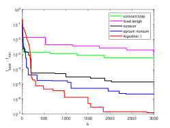
(a) $n=2$ and $m=10$

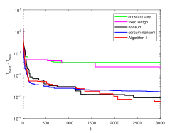
(b) $n=5$ and $m=30$

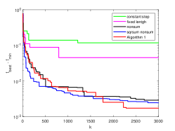
(c) $n=10$ and $m=50$

Figure 1: Best value of $f(x^{k})-f^{*}$ (using log. scale) for Algorithm 3 and each step size in Table 1.

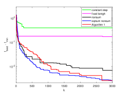
(a) $n=20$ and $m=100$

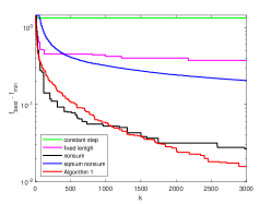
(b) $n=50$ and $m=150$

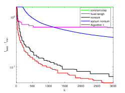
(c) $n=100$ and $m=500$

Figure 2: Best value of $f(x^{k})-f^{*}$ (using log. scale) for Algorithm 3 and each step size in Table 1.

	Algorithm 3		constant step		fixed length
	$f_{best}-f_{min}$	$it_{best}$	$f_{best}-f_{min}$	$it_{best}$	$f_{best}-f_{min}$	$it_{best}$
$n=2$, $m=10$	1.23289e-07	2838	5.9329e-04	1863	1.29047e-03	2990
$n=5$, $m=30$	6.11231e-04	2872	0.038322	858	0.0239323	1579
$n=10$, $m=50$	1.73369e-03	2286	0.118048	1215	0.0455682	795
$n=20$, $m=100$	2.63594e-03	2675	0.389903	235	0.169888	2698
$n=50$, $m=150$	0.0157351	2895	1.32626	25	0.37411	2175
$n=100$, $m=500$	0.0483826	2696	1.59047	2	0.613463	2820

Table 2: Iteration where each algorithm attains the best value of $f(x^{k})-f^{*}$.

	nonsum		sqrsum nonsum
	$f_{best}-f_{min}$	$it_{best}$	$f_{best}-f_{min}$	$it_{best}$
$n=2$, $m=10$	1.4022e-05	2034	2.1927e-06	2363
$n=5$, $m=30$	9.0404e-04	2412	1.7e-03	2949
$n=10$, $m=50$	2.90217e-03	2686	2.4701e-03	2765
$n=20$, $m=100$	6.96234e-03	2699	2.57007e-03	2959
$n=50$, $m=150$	0.0266287	2978	0.205205	2964
$n=100$, $m=500$	0.0646978	2868	0.39232	2972

Table 3: Iteration where each algorithm attains the best value of $f(x^{k})-f^{*}$.

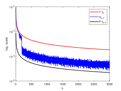
(a) $n=2$ and $m=10$

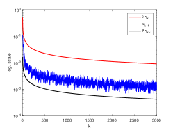
(b) $n=5$ and $m=30$

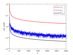
(c) $n=10$ and $m=50$

Figure 3: Behavior of the sequences $\{\alpha_{k}\}$ and $\{\gamma_{k}\}$ (using log. scale) for Algorithm 3.

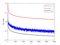
(a) $n=20$ and $m=100$

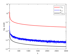
(b) $n=50$ and $m=150$

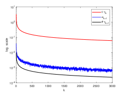
(c) $n=100$ and $m=500$

Figure 4: Behavior of the sequences $\{\alpha_{k}\}$ and $\{\gamma_{k}\}$ (using log. scale) for Algorithm 3.

4.2 Fermat-Weber location problem

The experiment of this section is the well known Fermat-Weber location problem; see for instance Brimberg [3]. Let $a_{1},\ldots,a_{m}$ be given points in $\mathbb{R}^{n}$. The Fermat-Weber location problem is to solve the following minimization problem

$$\min_{x\in\mathbb{R}^{n}}f(x)=\sum_{i=1}^{m}w_{i}||x-a_{i}||.$$

In our particular application, we consider the data points $a_{i}$, for $i=1,\ldots,27$, given by the coordinate of the cities which are capital of all 26 states of Brazil and Brasília (the Federal District, capital of Brazil). We take equally weights for all $a_{i}$, namely, $w_{i}=1$, $i=1,\ldots,27$, and consider the integer part of the coordinates converting it from positive to negative to match with the real data. Our goal is to find a point that minimizes the sum of the distances to the given points representing the cities in order to see how distance is such a point from Brasília (the capital of Brazil). We denote by

$$f_{min}=312.9232964118977,\qquad x_{min}=(-45.9630806884547,-12.7465709013343)$$ (21)

the solution found by the MATLAB package CVX; see [7, 8]. As mentioned in the beginning of this section, we perform Algorithm 3 and other four subgradient methods each of them with different step sizes $\alpha_{k}$ described in Table 1. All the methods start from the same initial point and they stop at $k=200$ iterates. In Algorithm 3, we take $\zeta=2$ in the definition of $\{\gamma_{k}\}$.

In Table 4, we present in the first two columns the solution $x^{*}=(x_{1}^{*},x_{2}^{*})$ found by each method, in the third column the best value to $|f_{best}-f_{min}|$, where $f_{best}$ stands to the best value of the objective function for each method and $f_{min}$ is given by (21). The last column shows the iterate $it_{best}$ in which the best value $|f_{best}-f_{min}|$ was attained. As we can notice, Algorithm 3 and the subgradient method with constant step size found a better solution compared to the solution known ($f_{min}$ and $x_{min}$) than the other methods. However, Algorithm 3 found its best value in 29 iterates while the subgradient method with constant step size takes 90 iterates to attain its best value. The performance of each method is presented in Figure 5b showing the efficiency of the Algorithm 3 for this example. In Figure 5a, we present the data of this example as well as the iterates of the Algorithm 3 and the solution found by the method.

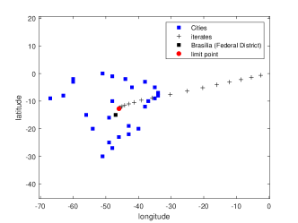
(a) Running Algorithm 3.

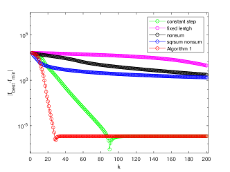
(b) Performance of the methods (in log. scale).

Figure 5: Subgradient methods for solving the Fermat-Weber location problem.

	$x_{1}^{*}$	$x_{2}^{*}$	$|f_{best}-f_{min}|$	$it_{best}$
Algorithm 3	-45.963064141347097	-12.746621089909885	2.66879e-07	29
constant step	-45.963064140711523	-12.746621088320897	2.42824e-08	90
fixed length	-38.605444422335090	-9.623064720309808	40.7379	200
Nonsum	-43.842367512948982	-11.429938434104701	4.02647	200
Sqrsum nonsum	-44.521197252917077	-11.740733447040283	1.9869	200

Table 4: Solution found for the Fermat-Weber location problem.

5 Conclusions

In this paper we have presented a subgradient method with a non-monotone line search for the minimization of convex functions with simple convex constraints. The non-monotone line search allows the method to adaptively select step sizes. As preliminary numerical tests show, this method performs better than the standard subgradient method with prefixed step sizes, which we hope to motivate further research on this subject.

References

• [1] A. Beck. First-Order Methods in Optmization. Society for Industrial and Applied Mathematics-SIAM and Mathematical Optimization Society, 1st edition, 2017.
• [2] D. P. Bertsekas. Nonlinear programming. Athena Scientific Optimization and Computation Series. Athena Scientific, Belmont, MA, second edition, 1999.
• [3] J. Brimberg. The Fermat—Weber location problem revisited. Math. Program. 71:71–76, 1995.
• [4] P. L. Combettes. Quasi-Fejérian analysis of some optimization algorithms. In Inherently parallel algorithms in feasibility and optimization and their applications (Haifa, 2000), volume 8 of Stud. Comput. Math., pages 115–152. North-Holland, Amsterdam, 2001.
• [5] Y. M. Ermol’ev. Methods of solution of nonlinear extremal problems. Cybernetics, 2(4):1–14, 1966.
• [6] J.-L. Goffin and K. C. Kiwiel. Convergence of a simple subgradient level method. Math. Program., 85(1, Ser. A):207–211, 1999.
• [7] M. Grant and S. Boyd. Cvx: Matlab software for disciplined convex programming, version 2.1, 2014.
• [8] M. C. Grant and S. P. Boyd. Graph implementations for nonsmooth convex programs. In Recent advances in learning and control, volume 371 of Lect. Notes Control Inf. Sci., pages 95–110. Springer, London, 2008.
• [9] G. N. Grapiglia and E. W. Sachs. On the worst-case evaluation complexity of non-monotone line search algorithms. Comput. Optim. Appl., 68(3):555–577, 2017.
• [10] L. Grippo, F. Lampariello, and S. Lucidi. A nonmonotone line search technique for Newton’s method. SIAM J. Numer. Anal., 23(4):707–716, 1986.
• [11] J.-B. Hiriart-Urruty and C. Lemaréchal. Convex Analysis and Minimization Algorithms I. Springer, Berlin, Heidelberg, 1993.
• [12] J.-B. Hiriart-Urruty and C. Lemaréchal. Convex analysis and minimization algorithms. I, volume 305 of Grundlehren der Mathematischen Wissenschaften [Fundamental Principles of Mathematical Sciences]. Springer-Verlag, Berlin, 1993. Fundamentals.
• [13] K. C. Kiwiel. Methods of descent for nondifferentiable optimization, volume 1133 of Lecture Notes in Mathematics. Springer-Verlag, Berlin, 1985.
• [14] K. C. Kiwiel. Convergence of approximate and incremental subgradient methods for convex optimization. SIAM J. Optim., 14(3):807–840, 2003.
• [15] N. Krejic, N. K. Jerinkic, and T. Ostojic. Spectral projected subgradient method for nonsmooth convex optimization problems. arXiv preprint arXiv:2203.12681, pages 1–17, 2022.
• [16] M. Loreto and A. Crema. Convergence analysis for the modified spectral projected subgradient method. Optim. Lett., 9(5):915–929, 2015.
• [17] M. Loreto, Y. Xu, and D. Kotval. A numerical study of applying spectral-step subgradient method for solving nonsmooth unconstrained optimization problems. Comput. Oper. Res., 104:90–97, 2019.
• [18] A. Nedić and D. Bertsekas. Convergence rate of incremental subgradient algorithms. In Stochastic optimization: algorithms and applications (Gainesville, FL, 2000), volume 54 of Appl. Optim., pages 223–264. Kluwer Acad. Publ., Dordrecht, 2001.
• [19] A. Nedić and D. P. Bertsekas. The effect of deterministic noise in subgradient methods. Math. Program., 125(1, Ser. A):75–99, 2010.
• [20] Y. Nesterov. Subgradient methods for huge-scale optimization problems. Math. Program., 146(1-2, Ser. A):275–297, 2014.
• [21] B. T. Polyak. Introduction to optimization. Translations Series in Mathematics and Engineering. Optimization Software, Inc., Publications Division, New York, 1987. Translated from the Russian, With a foreword by Dimitri P. Bertsekas.
• [22] E. W. Sachs and S. M. Sachs. Nonmonotone line searches for optimization algorithms. Control Cybernet., 40(4):1059–1075, 2011.
• [23] N. Z. Shor. Minimization methods for nondifferentiable functions, volume 3 of Springer Series in Computational Mathematics. Springer-Verlag, Berlin, 1985. Translated from the Russian by K. C. Kiwiel and A. Ruszczyński.
• [24] H. Zhang and W. W. Hager. A nonmonotone line search technique and its application to unconstrained optimization. SIAM J. Optim., 14(4):1043–1056, 2004.