Arbitrary Bit-width Network: A Joint Layer-Wise Quantization and Adaptive Inference Approach

Abstract.

Conventional model quantization methods use a fixed quantization scheme to different data samples, which ignores the inherent “recognition difficulty” differences between various samples. We propose to feed different data samples with varying quantization schemes to achieve a data-dependent dynamic inference, at a fine-grained layer level. However, enabling this adaptive inference with changeable layer-wise quantization schemes is challenging because the combination of bit-widths and layers is growing exponentially, making it extremely difficult to train a single model in such a vast searching space and use it in practice. To solve this problem, we present the Arbitrary Bit-width Network (ABN), where the bit-widths of a single deep network can change at runtime for different data samples, with a layer-wise granularity. Specifically, first we build a weight-shared layer-wise quantizable “super-network” in which each layer can be allocated with multiple bit-widths and thus quantized differently on demand. The super-network provides a considerably large number of combinations of bit-widths and layers, each of which can be used during inference without retraining or storing myriad models. Second, based on the well-trained super-network, each layer’s runtime bit-width selection decision is modeled as a Markov Decision Process (MDP) and solved by an adaptive inference strategy accordingly. Experiments show that the super-network can be built without accuracy degradation, and the bit-widths allocation of each layer can be adjusted to deal with various inputs on the fly. On ImageNet classification, we achieve 1.1% top1 accuracy improvement while saving 36.2% BitOps.

1. Introduction

Model quantization is one of the most promising compression methods for deploying deep neural networks on resource-limited devices. It leverages the intrinsic robustness of neural networks in preserving their expressiveness even after reducing their bit-width. For example, an 8-bit network can typically increase the inference speed by 4$\times$ compared to a full-precision (32-bit) network, with 4$\times$ less storage space and negligible accuracy degradation Intel Corp. (2019). Classical quantization methods can be divided into two categories, independent methods and joint methods.

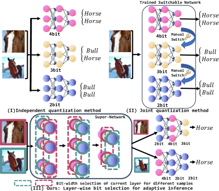
Figure 1. Inference process of a three-layer toy network with two input samples under different methods. (I) Independent method cannot directly perform bit-width switching without retraining. (II) Joint method gets a switchable network that can switch bit-width of the entire network manually during inference. They fail to exploit a fine-grained layer-wise quantization and cannot provide a data-dependent adaptive inference scheme. (III) Our method enables adaptive inference by training a super-network that can switch bit-widths per layer and by constructing a runtime inference framework to select bit-widths to each layer according to different input data. It can perceive the sample differences during inference and provide a fine-grained bit-width adjustment.

Independent methods (a.k.a quantization-aware training) Zhou et al. (2016); Esser et al. (2020); Wang et al. (2019) tie the model to a specific quantization scheme during training, making it impossible to change the bit-width of a quantized model during inference without costly retraining. On the other hand, joint methods Jin et al. (2020); Bulat and Tzimiropoulos (2021); Guerra et al. (2020); Du et al. (2020); Yu et al. (2019) allow the entire network to be switched to other bit-widths manually without retraining. However, they fail to fully exploit different bit-width sensitivity at the layer level, but ignore different layers that have different sensitivities to quantization Dong et al. (2019); Wang et al. (2019). For instance, Cai and Vasconcelos (2020) finds in the Inception module of the GoogleNet Szegedy et al. (2015), the first 1$\times$1 kernel size layer has almost the same amount of computation as the last 5$\times$5 kernel size layer, but the former causes about 2% more absolute accuracy degradation than the latter at low bit-width quantization. This reveals that it is not necessary to use the same high bit-width for all layers of a network; instead, it is vital to use high bit-width only for those layers that are quantization sensitive, while let other layers use low bit-width as a way to achieve better efficiency.

It has been widely observed that different inputs require different computational consumption Huang et al. (2018); Wu et al. (2018a); Rao et al. (2018), which is caused by the inherent “recognition difficulty” differences between various inputs. For example, an image with a clear and central object should use less computational resource (or bit-widths, in our case) than another one with a blurred object located at the edge. However, classical quantization methods cannot adjust the bit-width adaptively to fit this observation. Independent methods can only use a fixed quantization scheme for all samples, because this scheme is usually assigned before training and cannot be changed during inference. Joint methods can switch the bit-width of the entire network, but requires manual operation. In other words, they still cannot perceive the sample differences, so they are not adaptive inference methods either. Besides, and the most important thing is, that joint methods adjust the bit-width at a network level instead of at a praised layer level. Modern networks generally have dozens or even hundreds of layers. As we discussed above, the granularity of bit-width switching for the entire network is too coarse, which undoubtedly causes efficiency loss. Therefore, to achieve better efficiency and accuracy trade-off, our core idea is to adaptively feed different data samples with different quantization schemes at a layer level during inference. For example, on some layers, only samples that are difficult to recognize are assigned high bit-widths to ensure prediction accuracy. In contrast, those samples that are easy to recognize are assigned low bit-widths to reduce computation overhead. The difference between the classical quantization approaches and ours is illustrated in Fig. 1. The major challenges to realize this come from two perspectives.

(1) Exponentially increasing training space: Consider an $L$-layers network with $n$ optional bit-widths per layer, the number of possible quantization schemes (combinations of layers and bit-widths) is $n^{L}$, corresponding to $n^{L}$ subnets, while the joint methods only have $n$ subnets. For example, a ResNet34 with 4 bit-width options = $\{2,3,4,8\}$ per layer can generate $4^{34}\approx 2.9\times 10^{20}$ potential subnets in our training space. Obviously, it is impractical to train so many subnets separately, as it takes several GPU days to train only a single subnet Zhu et al. (2018), apart from the unacceptable storage overhead. A feasible solution is to train a single weight-shared “super-network” that contains all subnets, rather than training all networks individually. However, training in such an exponential space is non-trivial, as the space is too huge to be optimized effectively. As we will discuss later, a simple incremental version of the previous joint methods Jin et al. (2020); Bulat and Tzimiropoulos (2021) triggers a severe accuracy degradation due to a dramatic increase in the number of subnets.

(2) Exponentially increasing decision space: Even with a weight-shared network, it is still challenging to determine the optimal bit-width for each layer during inference, since the decision space also grows exponentially with the deepening of layers. Simple brute force searching or random sampling to select subnets leads to sub-optimal performances, because of its excessive time complexity or its obliviousness to different input data. Naively training a decision network by collecting the accuracy and computation cost under different bit-width configurations offline is also not feasible, considering the complexity of this problem.

In this paper, we present the first work to efficiently train a layer-wise quantizable network with adaptive ultra-low bit-widths during inference. Concretely, we divide our core idea into two tractable subproblems in the training space and runtime decision making space, corresponding to the two challenges mentioned above.

To efficiently train the super-network that can support multiple bit-widths at the layer level, we carefully analyze the most important factors affecting the performance of the super-network, and introduce two magic codes to train it effectively. We further propose two key techniques called knowledge ensemble and knowledge slowdown to stabilize the training process, resulting in a meaningful performance improvement.

To determine the proper configurations of each layer at runtime for various inputs, we model the optimal bit-width selection problem as a Markov Decision Process (MDP), and build a deep reinforcement learning (DRL) framework to make the online decisions under different inputs. By this means, we are able to solve the problem that classic quantization methods cannot perceive the sample differences.

In summary, our contributions are as follows:

• We propose a novel approach to train a layer-wise quantizable super-network, which only stores a single model (i.e., the weights of different bit-widths are derived from the same stored weights, rather than stored independently) that can switch to arbitrary bit-widths at runtime for any layer. This greatly increases the network’s runtime flexibility, providing a foundation for input-aware dynamic inference without loss of accuracy. Compared to joint training Jin et al. (2020); Du et al. (2020); Yu et al. (2019); Guerra et al. (2020), the top-1 accuracy on ImageNet classification improves by up to 4.1%, and we achieve that in a much more hard-to-optimize training space that is $n^{L-1}$ times larger than them.

• We propose a DRL-based framework to pick input-aware subnets from the trained super-network. The bit-width selection decision of each layer is modeled as an MDP. Accordingly, we train a DRL agent (a very lightweight network) that can achieve adaptively inference strategy to select the bit-width of each layer to reconcile the trade-off according to different inputs. On ImageNet classification, we improve 1.1% top-1 accuracy while using only 63.8% BitOps compred to the data-independent quantization scheme AutoQ Lou et al. (2019).

2. Related Work

2.1. Neural Network Quantization

Neural network quantization is effectively used to reduce the model storage and running overhead. Some are concerned about training a ultra-low precision model by using uniform quantization bit-width across the entire network Zhou et al. (2016); Baskin et al. (2021); Esser et al. (2020); Zhang et al. (2018); Li et al. (2016); Rastegari et al. (2016); Choi et al. (2018). Others focus on using mixed-precision quantization for different layers. That is, the bit-widths of each layer are not exactly equal. Since different layers always exhibit different redundancy, that can greatly improve the performance of the network, avoiding forcing less sensitive layers to use higher bit-widths Wu et al. (2018b); Wang et al. (2019); Guo et al. (2020); Dong et al. (2019). All their work already determines the bit-width of the network during training. Without retraining, it is impossible to switch the bit-width during inference.

2.2. Dynamic Neural Networks

Dynamic neural networks are a type of neural networks that can change their architectures in response to different inputs. Since not all input samples require the same amount of computation to produce plausible prediction results, the early-exit mechanism is proposed in Huang et al. (2018); Fang et al. (2020); Kaya et al. (2019); Teerapittayanon et al. (2016). This allows easy-to-compute samples to produce prediction results in the front layer of the network, thus avoiding additional computational consumption in subsequent layers. Wu et al. (2018a); Veit and Belongie (2018); Wang et al. (2018); Shen et al. (2020) propose a more flexible way of dynamically adjusting the computational graph by using either a controller or a decision gate to decide block by block whether to skip it or execute it (with full-precision or lower bit), rather than skipping all layers after a decision point directly. Corresponding to the dynamic adjustment of the network depth (number of layers) is the dynamic adjustment of the network width (number of channels) Chen et al. (2020); Liu et al. (2017); Lin et al. (2017), which is due to the fact that CNNs usually have enough redundancy in the channels to allow different pruning strategies to be generated at runtime based on different inputs.

2.3. Weight-Shared Networks

Weight-shared networks Jin et al. (2020); Yu and Huang (2019); Bulat and Tzimiropoulos (2021); Guerra et al. (2020); Du et al. (2020); Yu et al. (2019) use a single set of weights to support multi-scale inference or flexible deployment without storing separate models. Unlike dynamic neural networks, during training, such networks are usually not constrained by the computational resources of deployment time and are therefore more flexible. The works in Jin et al. (2020); Du et al. (2020); Yu et al. (2019); Guerra et al. (2020); Bulat and Tzimiropoulos (2021) that focus on quantization are most similar to ours, in which the bit-width of their trained networks can be switched at inference time without retraining. Nevertheless, Jin et al. (2020); Du et al. (2020); Yu et al. (2019); Guerra et al. (2020) use the same bit-width for the whole network, ignoring that layer’s sensitivity to quantization is quite different. In other words, they do not have the ability of runtime mixed-precision. Bit-Mixer Bulat and Tzimiropoulos (2021) trains a meta network with the ability of layer-wise switchable quantization level but treats all subnets equally during training, while the huge variability in convergence speed between subnets can lead to convergence to sub-optimal eventually. Consequently, each of the specific subnets requires tens of epochs for fine-tuning on the full training set to recover to normal accuracy, which is also a common drawback of weight-shared networks Cai et al. (2019); Yu et al. (2020). Considering a large dataset like ImageNet, the fine-tuning time for just a single subnet can take tens of GPU hours.

In this paper, we have carefully analyzed the most important factors affecting the weight-shared network performance and discovered a new training method. In this way, the accuracy of runtime mixed-precision on ImageNet classification can be improved significantly, the performance of our super-network can even reach the level of the separately trained networks. Moreover, the empirical results also show that the specific subnets no longer require costly fine-tuning to recover accuracy.

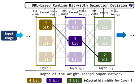
Figure 2. The overall framework of ABN.

3. Our Approach

The overall framework of ABN is shown in Fig. 2. Briefly, the weight-shared super-network is composed of a large number of subnets with the combination of layers and corresponding bit-widths. Each of the subnets can serve as a candidate for the given input data. Based on that, the DRL agent makes runtime bit-widths selection decisions layer-by-layer to determine the picked subnet for different input data, fully exploiting the advantage of ultra-low bit-widths quantization and dynamic inference.

In this section, we first discuss how to train the layer-wise quantizable super-network that supports runtime layer-wise granularity bit-widths allocation, with only one single weight-shared model to be stored. During inference, each layer of the super-network can be allocated an ultra-low bit-width ($\leq$ 8) to construct a specific subnet. Then, we devise the DRL-based framework to select bit-width for each layer at runtime dynamically. Thus, different input data can produce a series of different bit-width selections as the input-aware subnets, achieving adaptive inference consequently.

3.1. Quantizable Super-Network Training

3.1.1. Quantization Preliminary

For a set of bit-widths $\mathbb{B}=\{b_{max},\\ b_{1},...,b_{min}\}$, we expect to find a weight-shared network that can switch each layer to any bit-widths $b\in\mathbb{B}$ at runtime. Namely, the weights $W$ and activations $x$ of a certain layer are both quantized to $\widehat{W_{b}}$ and $\widehat{x_{b}}$ under $b$ bit-width. To this end, we extend the traditional independent quantization training method LSQ Esser et al. (2020). The weights are quantized with:

$$\widehat{W}_{b}=s_{b}^{W}\times\lfloor clip(\frac{W}{s_{b}^{W}},Q_{b},P_{b})\rceil$$ (1a)

$$\widehat{W}_{b}=s_{b}^{W}\times\lfloor clip(\frac{\widehat{W}_{b_{max}}}{s_{b}^{W}},Q_{b},P_{b})\rceil,$$ (1b)

where Eq. 1a (Round Operator) requires the network to be stored as full-precision but guarantees sufficient accuracy, and Eq. 1b (Weights Alignment) allows the network to be stored directly in bit-widths of $b_{max}$ but with a small loss of accuracy. For Eq. 1b, $\widehat{W}_{b_{max}}=W$ when $b=b_{max}$, which means the weights are obtained from the full-precision $W$ only when $b=b_{max}$. The difference between these two formulas and the Floor Operator used in Jin et al. (2020); Bulat and Tzimiropoulos (2021) is illustrated in Fig. 3.

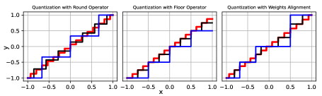
Figure 3. Illustration of different quantization schemes.

Beyound that, for activations, we use:

$$\widehat{x_{b}}=s_{b}^{x}\times\lfloor clip(\frac{x}{s_{b}^{x}},Q_{b},P_{b})\rceil.$$ (2)

Specifically, $s_{b}^{W}$ and $s_{b}^{x}$ are the learned step size scale factor of weights and activations that need be trained for this layer. $\lfloor\cdot\rceil$ indicates that the input value is rounded to the nearest integer. $clip(r_{0},r_{1},r_{2})$ indicates that $r_{0}$ will be secured between the minimum value $r_{1}$ and the maximum value $r_{2}$. Given a bit-width $b$ for this layer, $Q_{b}$ and $P_{b}$ are fixed. For weights, $Q_{b}=-2^{b-1}$ and $P_{b}=2^{b-1}-1$; for activations, $Q_{b}=0$ and $P_{b}=2^{b}-1$.

In order to solve the problem of shifting activation distribution between different bit-widths, we use a layer-wise switchable batch normalization (BN) layer Jin et al. (2020); Yu and Huang (2019); Ioffe and Szegedy (2015). To be specific, we replace the original single BN layer that follows after each convolutional layer with the bit-specified BN layers. Namely, a layer with $n$ bit-width options has $n$ BN layers corresponding to these $n$ bit-width options. Thus, for each convolution layer, when its allocated bit-width $b_{0}$ switches to $b_{1}$, its corresponding $s_{b_{0}}$, $Q_{b_{0}}$, $P_{b_{0}}$ and BN layer BN${}_{b_{0}}$ switch to $s_{b_{1}}$, $Q_{b_{1}}$, $P_{b_{1}}$ and BN${}_{b_{1}}$ accordingly.

3.1.2. Random Sampling

Our goal here is to find a single set of weights that will support switching the quantization level of each layer at runtime in a re-training-free fashion. Suppose the expected weights of the “super-network” is $W_{S}$; the aggregation of all possible configurations of bit-width is $\mathcal{C}$; and each configuration corresponds to a subnet. It is obvious that we cannot train all subnets simultaneously due to the GPU memory is finite. Thus we first investigate an intuitive approach inspired by the one-shot NAS Guo et al. (2020), which not only trains the weights $W(j)$ of naive joint training, but also appends an additional random sampling process, i.e., randomly sampling a bit-width configuration $c\in\mathcal{C}$ at each step. This can be expressed as:

$$W_{S}=\operatorname*{arg\,min}_{W}\mathbb{E}_{c\sim{U(\mathcal{C})}}[\mathcal{L}_{train}(W(j),W(c))].$$ (3)

In this way, it is expected that the trained network will have the ability of runtime mixed-precision (layer-wise mutable bit-widths at runtime). The result is shown in Tab. 1.

Table 1. Top1 accuracy (%) of two training strategies of ResNet18 on ImageNet. “Mixed” refers to randomly selecting bit-widths to each layer during inference to test the network’s performance of runtime mixed-precision.

Method	4 Bit	3 Bit	2 Bit	Mixed
Independent Training (LSQ)	69.6	68.9	66.3	-
Random Sampling	69.0	68.3	64.7	66.3

Although the trained network can change the bit-width during inference without retraining, it shows a significant accuracy degradation compared to independent training. In the most serious case (i.e., 2 Bit), it has 1.6% top1 accuracy degradation. That suggests that it is still something more than intuition that needs to be studied. In fact, the random sampling method is more like an incremental version of Jin et al. (2020) that treats all subnets equally. A similar approach is used in Bulat and Tzimiropoulos (2021) to make the network obtain runtime mixed-precision capability. As the results show, this intuitive approach causes the network to sub-optimal converged performance. Therefore, the training method of super-network should be analyzed carefully, as we will discuss in 3.1.3.

3.1.3. Analysis of Training Efficiency

Consider a convolution operation under $b$ bits:

$$y_{b}=(W+n_{b}^{w})\odot(x+n_{b}^{x}),$$ (4)

where $W$ and $x$ are the weights and activations, $n_{b}^{w}$ and $n_{b}^{x}$ are the quantization noise of weights and activations introduced by $b$ bits. Reducing the bit-width leads to an increase in quantization noise Zhou et al. (2018). And as shown in Fig. 4, the variance of quantized layers shows a negative correlation with bit-widths. Namely, as the bit-width decreases, the error increases. Thus the absolute error of this layer can be expressed in the form of the following inequality:

$$|y-y_{b_{max}}|=0\leq|y-y_{k}|\leq|y-y_{b_{min}}|.$$ (5)

In particular, we can deem $y\approx y_{b_{max}}$, because the highest precision output is by $y_{b_{max}}$; $y_{k}$ is the output of this layer under $k$ bit-width mode, $b_{min}\leq k\leq b_{max}$. The inequation indicates that performance in all subnets is bounded by the maximum and minimum bit-width mode. Optimizing the lower and upper bound can improve the accuracy of all subnets subtly. Since cross-entropy (CE) is the unmodifiable criterion of lower bound, thus the overall performance is actually limited by the upper bound bit-width mode $b_{min}$. That reveals the importance of the subnet whose bit-width is $b_{min}$ at each layer. That is, improving the accuracy of this crucial subnet can potentially improve the overall performance of the entire super-network.

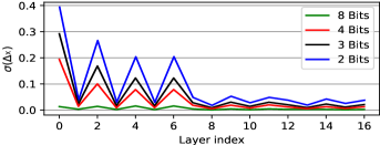
Figure 4. The variance of the activations for the 16 convolutional layers of ResNet18. It can be found that the higher the bits, the smaller the variance. $\Delta x=x-\hat{x}_{b}$.

As shown in Tab. 1, runtime mixed-precision performance of the super-network can be obtained sketchily by adding a random sampling process. Accordingly, although it is not necessary to train all subnets at the same time, the number $k$ of random sampling is still non-trivial. Too little sampling (e.g., once) may result in some subnets not being adequately trained; too much sampling results in too much computation and may lead to intense internal conflicts within the weight-shared super-network, affecting the convergence seriously. The effect of different random sampling numbers $k$ will be further demonstrated in the experiment.

To sum up, the two magic codes of efficiently training a layer-wise quantizable super-network are to improve the accuracy of the crucial subnet and to randomly assign bit-width per layer during training. For the former, we propose two techniques called knowledge ensemble and knowledge slowdown to boost the accuracy of the $b_{min}$ bit-width mode. For the latter, we experimentally explore the effect of the number of random sampling on the super-network.

Notice that in order to ensure contextual consistency in this paper for clear expression, we logically divide the training process of the super-network into four continuous sub-stages for later description, which also corresponds to different subnets, namely:

(I) A maximum bit-width uniform stage $S_{max}^{u}$ (i.e., each layer is equally allocated the bit $b_{max}$).

(II) A middle bit-width uniform stage $S_{mid}^{u}$ (i.e., each layer is allocated an equal bit, except for $b_{min}$ or $b_{max}$).

(III) $k$ random nonuniform sampling stage $S_{rand}^{n}$ (i.e., the bit of each layer is randomly allocated).

(IV) A minimum bit-width uniform stage $S_{min}^{u}$ (i.e., each layer is equally allocated the bit $b_{min}$).

3.1.4. Knowledge Ensemble

Knowledge distillation (KD) is the most famous means to train a weight-shared network Hinton et al. (2015); Du et al. (2020); Anil et al. (2018); Yu and Huang (2019), by using soft-lables of the highest accuracy subnet (i.e., $S_{max}^{u}$) as the “teacher” to guide other subnets (students). It can reduce the conflict between subnets and stabilize the training. However, KD does not work so well for the $S_{min}^{u}$ due to the extremely asymmetric convergence rate (EACR) between the maximum and minimum bit-width. We show that phenomenon in Fig. 5, where the EACR remains significant (about 10%) even after 10 epochs. Not only that, in experiments, we even observe a much severe missdistance in the early phases, with an accuracy gap of more than 30%.

Some researchers find that KD can lead the students to sub-optimal converged performance when the accuracy gap between teacher and students is too large Mirzadeh et al. (2020); Gao et al. (2021). Moreover, Frankle et al. (2019); Achille et al. (2017) have shown that the very early training time is much essential for the network, meaning such a severe gap might damage the overall performance at the essential early phases. Thus the naive KD is not suitable for guiding the crucial subnet anymore because Eq. 5 shows that if its performance is damaged, the overall performance is reduced.

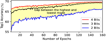
Figure 5. Asymmetric convergence rate of ResNet18 on ImageNet between different bit-widths, which shows a great gap between the 2-bits and 4-bits.

It is confirmed that multiple teachers can provide rich knowledge and then generate a much well-performed student You et al. (2017); Liu et al. (2020). Nevertheless, they all suffered the problem of regulating the importance between soft-labels generated by different teachers with different structures. Unlike them, we have numerous subnets with the same structure, which means the different importance of soft-labels due to different structures can be totally avoided. So that we can leverage these subnets as teachers to produce ensemble knowledge for distilling $S_{min}^{u}$. That is, we use a buffer $\mathcal{D}$ to store the output logits $y_{max}^{u}$, $y_{mid}^{u}$ and $y_{rand}^{n}$ of $S_{max}^{u}$, $S_{mid}^{u}$ and $S_{rand}^{n}$ respectively. Then, we use the average of all soft-labels in $\mathcal{D}$ to calculate the loss of $S_{min}^{u}$.

3.1.5. Knowledge Slowdown

To ensure knowledge ensemble could provide stable and reliable soft-labels, and further mitigate the extremely asymmetric convergence rate problem, we take inspiration from the value-based DRL algorithms Van Hasselt et al. (2016); Mnih et al. (2015). Specifically, we introduce a target network to produce soft-labels instead of using the one that is being trained (a.k.a the main natwork).

The core idea of knowledge slowdown is to generate soft-labels by using a network with the same structure as the main network, but with a slower pace of parameter updates. In this way, the main network changes from supervising the subnets and updating weights simultaneously to only performing weights updated. Thus, the above two processes of supervising and updating can radically decouple, making the training more stable. The parameters of the target network can be updated either by exponential moving average (EMA) or by copying directly at every C-step from the main network.

Hence, the loss function for each mini-batch $\bm{(x,y)}$ is as follows:

$$\left\{\begin{aligned} \mathcal{L}_{max}&=\mathcal{L}_{CE}(\bm{y_{max}^{u}},\bm{y}),\\ \mathcal{L}_{mid}&=\mathcal{L}_{KL}(\bm{y_{mid}^{u}},\hat{y}_{max}),\\ \mathcal{L}_{rand}&=\mathcal{L}_{KL}(\bm{y_{rand}^{n}},\hat{y}_{max}),\\ \mathcal{L}_{min}&=\mathcal{L}_{KL}(\bm{y_{min}^{u}},\frac{1}{\left|\mathcal{D}\right|}\sum\nolimits_{i\in\mathcal{D}}\bm{\hat{y_{i}}}),\end{aligned}\right.$$ (6)

where $\widehat{y}$ denote the soft-labels produced from the target network under different modes, $\mathcal{L}_{CE}$ is the cross-entropy (CE) loss and $\mathcal{L}_{KL}$ is the kullback–leibler (KL) loss.

3.2. Runtime Layer-wise Bit-width Selection

After obtaining the super-network, we start to consider the problem of making the layer-wise bit-width selection decision based on different input samples at runtime. In general, there are two ways to achieve this: the first way is to perform a one-time decision, i.e., for an input sample, a vector $\vec{v}$ is output at once, with each of its components corresponding to the bit-width of each layer; the second way is to carry out a step-by-step decision, i.e., the bit-widths are selected layer by layer for an input sample. Since the impact from quantization accumulates as the layers go deepened, we propose using the second way so that each decision is made sequentially.

For a given layer $l_{i}$, we want the bit-width $b$ for weights $W_{i}$ and activations $x_{i}$ that can achieve higher accuracy and lower computational consumption, which can be formed as the following objective:

$$\min_{b}\mathbb{E}[\mathcal{L}_{T}({q(W_{i},b)\odot q(x_{i},b)})-\mathcal{L}_{C}(l_{i},b)],$$ (7)

where $q(a,b)$ is the quantization function mentioned in Eq. 1 and Eq. 2 that quantizes the input tensor $W_{i}$ or $x_{i}$ to $b$ bit-width, $\odot$ is the convolution operation, $\mathcal{L}_{T}$ is the loss of the task (e.g., cross entropy), and $\mathcal{L}_{C}$ is the computational costs in this layer at bit-width $b$ (e.g., BitOps).

For an $L$-layers neural network with $n$ bit-widths for each layer, the time complexity of gathering the supervised configurations is $\mathcal{O}(\prod_{i=1}^{L}n)$. Due to this exponential time complexity, the objective function cannot be optimized directly using conventional supervised learning for the existing deep neural network with dozens or tens of layers.

To solve this, we first model the choice of optimal bit-width as a layer-by-layer MDP. Then, we build a DRL-based framework to make the step-by-step bit-width selection decision. The details of MDP are as follows.

3.2.1. State

We construct the state as an embedding vector, which consists of three parts as follows: (I) A fixed-length vector of input feature map of current layer. For the input feature map $\mathbf{F}_{i}\in\mathbb{R}^{c^{in}_{i}\times w_{i}\times h_{i}}$ of layer $l_{i}$, we first use the global pooling to make its dimension to $\mathbb{R}^{c^{in}_{i}}$, where $c^{in}_{i}$, $w_{i}$ and $h_{i}$ is the input channel number, width and height of layer $l_{i}$. After that, for different input channel number of different layers, we then use a fully-connected layer to project the pooled feature into a fix-length vector $\vec{f_{i}}$. (II) Layer index $i$. (III) The action of last layer $a_{i-1}$.

3.2.2. Action

The action $a$ is defined as the bit-width for layer $i$. Since we are mainly concerned with ultra-low bit-width ($\leq$ 8) and employ a layer-by-layer approach, a discrete action space is enough to determine the bit-width of each layer.

3.2.3. Reward Shaping

The reward should consider the accuracy and computational consumption of the super-network. Therefore we define $\mathcal{R}_{T}$ as the final accuracy of the task, and we expect it to be as high as possible, $\mathcal{R}_{C}(l_{i},b)$ is the computational consumption (BitOps) of layer $i$ under $b$ bit-width, where we prefer it to be as low as possible. So the reward of action $a_{j}$ for $i$-th layer is defined as:

$$r(a_{j})=\left\{\begin{array}[]{l}\mathcal{R}_{T}-\alpha\times\mathcal{R}_{C}(l_{i},a_{j}),\textrm{if the last layer (i = L)},\\ -\alpha\times\mathcal{R}_{C}(l_{i},a_{j}),\textrm{otherwise}\end{array}\right.$$ (8)

where $\alpha$ is the hyper-parameter that drives the trade-off between accuracy and computational consumption. To decide the action under current state $s_{i}$ for layer $i$, we leverage a Q-learning Mnih et al. (2015) method that define a action-value function of expected reward under certain action as $Q(s_{i},a_{j};\theta)$, where $\theta$ indicates the parameters of DRL agent. Then each optimal action $a_{t}$ for layer $i$ is the action that maximizes the action-value function, which can be described as $a_{t}=\arg\max_{a_{j}}Q(s_{i},a_{j};\theta)$. The loss function of the DRL agent can be formed by the Bellman equation:

$$\mathcal{L}(\theta)=(r+Q(s_{i+1},\arg\max_{a_{j}}Q(s_{i+1},a_{j};\theta);\theta^{\prime})-Q(s_{i},a_{t};\theta))^{2}.$$ (9)

Thus in our DRL framework, an input image will generate a series of states corresponding to the layers to be decided.

4. Experiments

In this section, we first evaluate the performance of the consistent training algorithm of the super-network on ImageNet classification. Next, we conduct experiments on the DRL-based runtime bit-width selection. We conducted experiments of ResNet18/34/50 He et al. (2016), and a compact architecture MobileNet Howard et al. (2017) on ImageNet 2012 Russakovsky et al. (2015) to verify the performance of ABN.

4.1. Implementation Details

For the super-network, we use the pre-trained model as initialization, and we keep the first and last layer at full-precision Zhou et al. (2016). All ResNet models are trained for 160 epochs and MobileNet is trained for 130 epochs, both using the cosine scheduler and the SDG optimizer. The initial learning rate is 0.02 for all ResNet models, 0.01 for MobileNet. The weight-decay for all models is $10^{-4}$. We use the method in Bhalgat et al. (2020) to initialize the step size factor of weights. We use the basic data augmentation method. All training data are randomly cropped to 224$\times$224 and randomly flipped horizontally. The number of random sampling $k=2$. The parameters of the target network are updated by EMA from the main network, as EMA generally ensures the stability of RL training Srinivas et al. (2020).

The bit-width options are {4, 3, 2} for ResNet and {8, 6, 4} for MobileNet. These options are considered the fact that ultra-low bit-width ($\leq$4) quantization is much more difficult than high bit-width ($>$4), therefore if our method is available in the ultra-low bit-width it also can be generalized to higher bit-widths.

We observe the same non-convergence problem as Adabits Jin et al. (2020) when weights directly are quantized by using Eq. 1b for $b_{min}$ <3. Adabits addressed this by storing the weights to full-precision. To take a step further, we add an 8 bit-width mode as $S_{max}^{u}$ and then clip all subnets containing 8 bits after convergence, which reduces the storage footprint $4\times$ but causes a bit of degradation of accuracy. For a fair comparison, we provide the FP results trained by Eq. 1a.

The DRL agent is a very lightweight network with only 5 fully-connected layers, each with between 64 and 256 neurons. As a comparison, FLOPs of the DRL agent and ResNet18 are 0.15M and 1819M, respectively. To save training time, we sampled 10% data of ImageNet2012 training set for training the DRL agent. It is trained by the Adam optimizer with a learning rate of $10^{-6}$.

Table 2. Top-1 accuracy(%) on ImageNet for different super-networks. We implement both Eq. 1a and Eq. 1b for training, where Eq. 1a ensures higher accuracy and Eq. 1b reduces the storage footprint with a tiny accuracy degradation. The best results overall are bolded in each metric, and the underline is the best result of all baselines. “-” indicates that the “Mixed” mode is not supported. Please note that “Independent Training” is the result of separate training of different bit modes. We provide this result to prove that only our training method meets or even exceeds the performance of separate training.

Network	Bit Mode	Ours	Ours (Eq. 1b)	Bit-Mixer Bulat and Tzimiropoulos (2021)	Adabits Jin et al. (2020)	APN Yu et al. (2019)	FQDQ Du et al. (2020)	Independent Training
ResNet18	4	69.8	68.9	69.2 (-0.6)	69.2 (-0.6)	67.9 (-1.9)	66.9 (-2.9)	69.6
	3	69.0	68.6	68.6 (-0.4)	68.5 (-0.5)		66.2 (-2.8)	68.9
	2	66.2	65.5	64.4 (-1.8)	65.1 (-1.1)	64.1 (-2.1)	62.1 (-4.1)	66.3
	Mixed	67.7	66.5	65.8 (-1.9)	-	-	-	-
ResNet34	4	74.0	73.5	72.9 (-1.1)	73.5 (-0.5)			73.8
	3	73.3	73.0	72.5 (-0.8)	73.0 (-0.3)			73.0
	2	71.7	70.3	69.6 (-2.1)	70.4 (-1.3)			71.1
	Mixed	72.5	71.6	70.5 (-2.0)	-			-
ResNet50	4	76.8	76.2	75.2 (-1.6)	76.1 (-0.7)	74.9 (-1.9)		76.6
	3	76.2	75.1	74.8 (-1.4)	75.8 (-0.4)	74.5 (-1.7)		75.8
	2	74.3	73.5	72.1 (-2.2)	73.2 (-1.1)	73.2 (-1.1)		73.5
	Mixed	75.5	74.3	73.2 (-2.3)	-	-		-
MobileNetV1	8	72.6	72.5		72.3 (-0.3)			72.7
	6	72.2	72.2		72.3 (+0.1)			72.3
	4	70.7	70.6		70.4 (-0.3)			70.7
	Mixed	71.2	71.1		-	-		-

4.2. Results for Super-Network

In Tab. 2, we report our results and compare them with other state-of-the-art quantization algorithms. Compared to independent/joint methods, our super-network surpasses the accuracy of uniform bit-width mode (i.e., the bit-width of each layer is equal) in most results. Compared to the recently proposed Bit-Mixer Bulat and Tzimiropoulos (2021), we also achieve a significant improvement in accuracy. In particular, on ResNet34 and ResNet50, our training method can improve mixed-precision accuracy by 2.0% and 2.3%. This is a good proof that when training the super-network, as we analyzed in the previous section, the crucial subnet should be treated specially, rather than treating all subnets equally.

Overall, we note that the top1 accuracy has improved by up to 4.1%, and even the average improvement is about 1.36%. In addition to the accuracy, the super-network also capable of assigning bit-widths for each layer during inference time, which provides the foundation for adaptive inference.

4.2.1. Fine-Tuning Subnets

To further verify that our training solution achieve good enough performance on specific subnets, we randomly sampled 20 subnets out of the super-network, using the fine-tuning settings in Yu et al. (2020) (LR = 0.01/0.001, 10/25 epochs on the full training set, etc.). As shown in Fig. 6, the accuracy transformation of these subnets after fine-tuning fluctuates only around $\pm$0.1%. This indicates that our training strategy results in relatively optimal performance for any subnets.

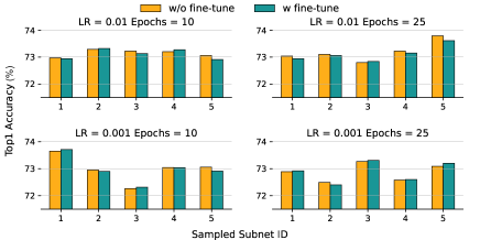
Figure 6. Top1 accuracy (%) of fine-tuning for ResNet34.

4.2.2. Results for Learned Factors

Fig. 7 shows the learned step size scale factors (learned factors) of different layer activations and weights of ResNet34. We find that the difference in learned factors between different bit-widths is relatively large for the same layer. This illustrates the importance of using a unique factor for each bit-width. Also, for a smaller bit-width (e.g., 2bit), our training algorithm gives a larger learned factor compared to a larger bit-width (e.g., 4bit) to make the quantized values more suitable for the distribution of the smaller bit-width.

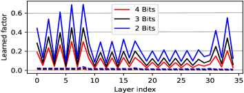
Figure 7. Learned factors for weights (dashed line) and activations (solid line) of ResNet34 on ImageNet.

4.2.3. Empirical Results for Random Sampling

Fig. 8 shows the results of random sampling $k$ with different values. We find that only random sampling once could lead to the runtime mixed-precision performance poorly. However, it is still very unwise to increase the number of random sampling heavily. Because that augments the training overhead and causes violent conflicts between sampled subnets, resulting in the network cannot be correctly converged. Results show that the mixed-precision performance of super-network is not positively correlated with the sampling number. Empirically, it has an optimal sampling number $k=2$, where the accuracy and training costs are both considered.

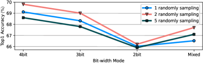
Figure 8. Top1 accuracy (%) with different $k$ of ResNet18 on ImageNet.

4.3. Results for Runtime Layer-wise Bit-width Selection

We verify the feasibility of the adaptive inference strategy on the ResNet18 super-network. The results of two DRL policies in Tab. 3 show that we achieved 0.8% accuracy improvement while using only 77.2% of the computational resources (BitOps) compared to baseline. Compared to the classical fixed mixed-precision scheme AutoQ, we also can achieve 1.1% accuracy improvement with 36.2% BitOps saving. In addition, since the DRL agent is actually a shallow network, its computation only accounts for about 2% of the overall network overhead. By replacing the four fully-connected layers we used with RNN, the computational cost of the DRL agent can be further reduced Wang et al. (2018).

Table 3. Result for runtime layer-wise bit-width selection. CCR indicates Constrained Computational Resources, which means the scenarios with limited computational resources, i.e., prioritizing fewer BitOps with as little impact on accuracy as possible. HAR indicates Higher Accuracy Requirement, which is suitable for scenarios requiring higher accuracy. “Acc.” means top1 accuracy (%). “$\Delta$Acc.” means the top1 accuracy improvement compared to the baseline. “W” denotes the bit-width of weights. “A” denotes the bit-width of activations. ^†: Layer-wise. ^↑: Nice cannot switch bit-width during inference. ^∗: Joint methods do not support adaptive inference, they need switch the bit-width of the entire network manually.

Method	Bit-width	Acc.	Acc.	BitOps
FQDQ∗ (baseline) Du et al. (2020)	3W3A	66.2	0	100.0%
AdaBits∗ Jin et al. (2020)	3W3A	68.5	+2.3	100.0%
Nice$\uparrow$ Baskin et al. (2021)	3W3A	67.7	+1.5	100.0%
APN∗ Yu et al. (2019)	4W4A	67.9	+1.7	177.7%
AutoQ† Lou et al. (2019)	Static Mixed	67.5	+1.3	$\sim$ 136.7%
Ours (DRL & CCR)	Runtime Mixed	67.0	+0.8	77.2%
Ours (DRL & HAR)	Runtime Mixed	68.6	+2.4	87.3%

We show the behavior of the CCR policy in Fig. 9. In CCR, the computational constraints are more stringent, so the DRL agent tends to allocate more low bit-widths. We observe that the DRL agent tends to use a large number of 2 and 3 bits to save BitOps. Also, the top layers have a high probability of using 4 bits, because these layers need high precision to extract low-level features. This suggests that the DRL agent adaptively takes different actions to reconcile computational consumption and accuracy for different inputs.

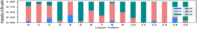
Figure 9. Action (Bit-width) selection probability of ResNet18 on ImageNet for CCR.

To further understand the behavior taken by the HAR policy, we divide the samples into two categories and visualize them in Fig. 10, namely easy samples (less bit-widths are allocated to save computation; about 90% of average BitOps) and hard samples (larger bit-widths are allocated to ensure accuracy; about 126% of average BitOps). We find that lower bit-widths are used for clear samples or samples where the entire object appears in the image, while higher bit-widths are used for blurred samples or where the target object is at the edge of the image.

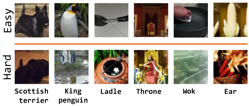
Figure 10. Visualization of easy (lower bit-widths are allocated by our DRL agent) and hard (higher bit-widths are allocated by our DRL agent) samples.

4.4. Ablation Studies for Knowledge Ensemble and Knowledge Slowdown

Tab. 4 shows that knowledge ensemble can boost the accuracy of 2-Bit and mixed 1.1% and 0.5%, respectively. With the combination of knowledge ensemble and knowledge slowdown, the accuracy of 2-Bit and mixed can be further improved by 2.4% and 1.3%, respectively. This demonstrates the effectiveness of these two techniques, which can alleviate the training difficulties caused by the exponential growth of training space and significantly boost the performance of the super-network.

Table 4. Top1 accuracy (%) results of ResNet34 on ImageNet for ablation study.

Knowledge ensemble	Knowledge slowdown	2 Bit	Mixed
✗	✗	69.3	71.2
✓	✗	70.4	71.7
✓	✓	71.7	72.5

5. Conclusion

This paper proposes the ABN to achieve layer-wise ultra-low bit-width adjustment adaptively according to specific input data. To do this, we solve two challenges. The first one is how to efficiently train one network that contains multiple possible bit-widths for each layer. The second one is how to determine the appropriate bit-width of each layer for different samples. For the former, we find the crucial subnet that has the greatest impact on the overall performance of the super-network, and propose two key technologies to push the performance of this lower bound. For the latter, we model the optimal bit-width selection problem as an MDP, and then propose a DRL-based adaptive inference strategy to pick input-aware subnets from the super-network. ABN can capture the differences across various inputs and then adjust bit-width on the fly, which makes it possible to guarantee sufficient accuracy while effectively reducing computational consumption.

References

- (1)
- Achille et al. (2017) Alessandro Achille, Matteo Rovere, and Stefano Soatto. 2017. Critical learning periods in deep neural networks. arXiv preprint arXiv:1711.08856 (2017).
- Anil et al. (2018) Rohan Anil, Gabriel Pereyra, Alexandre Passos, Robert Ormandi, George E Dahl, and Geoffrey E Hinton. 2018. Large scale distributed neural network training through online distillation. arXiv preprint arXiv:1804.03235 (2018).
- Baskin et al. (2021) Chaim Baskin, Evgenii Zheltonozhkii, Tal Rozen, Natan Liss, Yoav Chai, Eli Schwartz, Raja Giryes, Alexander M Bronstein, and Avi Mendelson. 2021. Nice: Noise injection and clamping estimation for neural network quantization. Mathematics (2021).
- Bhalgat et al. (2020) Yash Bhalgat, Jinwon Lee, Markus Nagel, Tijmen Blankevoort, and Nojun Kwak. 2020. Lsq+: Improving low-bit quantization through learnable offsets and better initialization. In IEEE Conference on Computer Vision and Pattern Recognition (CVPR).
- Bulat and Tzimiropoulos (2021) Adrian Bulat and Georgios Tzimiropoulos. 2021. Bit-Mixer: Mixed-precision networks with runtime bit-width selection. arXiv preprint arXiv:2103.17267 (2021).
- Cai et al. (2019) Han Cai, Chuang Gan, Tianzhe Wang, Zhekai Zhang, and Song Han. 2019. Once-for-All: Train One Network and Specialize it for Efficient Deployment. In International Conference on Learning Representations (ICLR).
- Cai and Vasconcelos (2020) Zhaowei Cai and Nuno Vasconcelos. 2020. Rethinking differentiable search for mixed-precision neural networks. In Proceedings of the IEEE/CVF Conference on Computer Vision and Pattern Recognition. 2349–2358.
- Chen et al. (2020) Jianda Chen, Shangyu Chen, and Sinno Jialin Pan. 2020. Storage Efficient and Dynamic Flexible Runtime Channel Pruning via Deep Reinforcement Learning. Advances in Neural Information Processing Systems (2020).
- Choi et al. (2018) Jungwook Choi, Zhuo Wang, Swagath Venkataramani, Pierce I-Jen Chuang, Vijayalakshmi Srinivasan, and Kailash Gopalakrishnan. 2018. Pact: Parameterized clipping activation for quantized neural networks. arXiv preprint arXiv:1805.06085 (2018).
- Dong et al. (2019) Zhen Dong, Zhewei Yao, Amir Gholami, Michael W. Mahoney, and Kurt Keutzer. 2019. HAWQ: Hessian AWare Quantization of Neural Networks With Mixed-Precision. In International Conference on Computer Vision (ICCV).
- Du et al. (2020) Kunyuan Du, Ya Zhang, and Haibing Guan. 2020. From Quantized DNNs to Quantizable DNNs. In 31st British Machine Vision Conference 2020 (BMVC).
- Esser et al. (2020) Steven K. Esser, Jeffrey L. McKinstry, Deepika Bablani, Rathinakumar Appuswamy, and Dharmendra S. Modha. 2020. Learned Step Size quantization. In 8th International Conference on Learning Representations (ICLR).
- Fang et al. (2020) Biyi Fang, Xiao Zeng, Faen Zhang, Hui Xu, and Mi Zhang. 2020. Flexdnn: Input-adaptive on-device deep learning for efficient mobile vision. In 2020 IEEE/ACM Symposium on Edge Computing (SEC). IEEE.
- Frankle et al. (2019) Jonathan Frankle, David J Schwab, and Ari S Morcos. 2019. The Early Phase of Neural Network Training. In International Conference on Learning Representations (ICLR).
- Gao et al. (2021) Mengya Gao, Yujun Wang, and Liang Wan. 2021. Residual error based knowledge distillation. Neurocomputing 433 (2021), 154–161.
- Guerra et al. (2020) Luis Guerra, Bohan Zhuang, Ian Reid, and Tom Drummond. 2020. Switchable precision neural networks. arXiv preprint arXiv:2002.02815 (2020).
- Guo et al. (2020) Zichao Guo, Xiangyu Zhang, Haoyuan Mu, Wen Heng, Zechun Liu, Yichen Wei, and Jian Sun. 2020. Single path one-shot neural architecture search with uniform sampling. In European Conference on Computer Vision (ECCV).
- He et al. (2016) Kaiming He, Xiangyu Zhang, Shaoqing Ren, and Jian Sun. 2016. Deep residual learning for image recognition. In IEEE Conference on Computer Vision and Pattern Recognition (CVPR). 770–778.
- Hinton et al. (2015) Geoffrey Hinton, Oriol Vinyals, and Jeff Dean. 2015. Distilling the knowledge in a neural network. arXiv preprint arXiv:1503.02531 (2015).
- Howard et al. (2017) Andrew G Howard, Menglong Zhu, Bo Chen, Dmitry Kalenichenko, Weijun Wang, Tobias Weyand, Marco Andreetto, and Hartwig Adam. 2017. Mobilenets: Efficient convolutional neural networks for mobile vision applications. arXiv preprint arXiv:1704.04861 (2017).
- Huang et al. (2018) Gao Huang, Danlu Chen, Tianhong Li, Felix Wu, Laurens van der Maaten, and Kilian Weinberger. 2018. Multi-Scale Dense Networks for Resource Efficient Image Classification. In International Conference on Learning Representations (ICLR).
- Intel Corp. (2019) Intel Corp. 2019. Intel Deep Learning Boost. https://software.intel.com/content/www/us/en/develop/topics/ai/deep-learning-boost.html. Accessed: 2021-07-08.
- Ioffe and Szegedy (2015) Sergey Ioffe and Christian Szegedy. 2015. Batch normalization: Accelerating deep network training by reducing internal covariate shift. In International conference on machine learning (ICML).
- Jin et al. (2020) Qing Jin, Linjie Yang, and Zhenyu Liao. 2020. AdaBits: Neural Network Quantization With Adaptive Bit-Widths. In IEEE Conference on Computer Vision and Pattern Recognition (CVPR).
- Kaya et al. (2019) Yigitcan Kaya, Sanghyun Hong, and Tudor Dumitras. 2019. Shallow-deep networks: Understanding and mitigating network overthinking. In International Conference on Machine Learning (ICML).
- Li et al. (2016) Fengfu Li, Bo Zhang, and Bin Liu. 2016. Ternary weight networks. arXiv preprint arXiv:1605.04711 (2016).
- Lin et al. (2017) Ji Lin, Yongming Rao, Jiwen Lu, and Jie Zhou. 2017. Runtime neural pruning. In Proceedings of the 31st International Conference on Neural Information Processing Systems (NeurIPS).
- Liu et al. (2020) Yuang Liu, Wei Zhang, and Jun Wang. 2020. Adaptive multi-teacher multi-level knowledge distillation. Neurocomputing (2020).
- Liu et al. (2017) Zhuang Liu, Jianguo Li, Zhiqiang Shen, Gao Huang, Shoumeng Yan, and Changshui Zhang. 2017. Learning efficient convolutional networks through network slimming. In International Conference on Computer Vision (ICCV).
- Lou et al. (2019) Qian Lou, Feng Guo, Minje Kim, Lantao Liu, and Lei Jiang. 2019. AutoQ: Automated Kernel-Wise Neural Network Quantization. In International Conference on Learning Representations (ICLR).
- Mirzadeh et al. (2020) Seyed Iman Mirzadeh, Mehrdad Farajtabar, Ang Li, Nir Levine, Akihiro Matsukawa, and Hassan Ghasemzadeh. 2020. Improved knowledge distillation via teacher assistant. In Proceedings of the AAAI Conference on Artificial Intelligence.
- Mnih et al. (2015) Volodymyr Mnih, Koray Kavukcuoglu, David Silver, Andrei A Rusu, Joel Veness, Marc G Bellemare, Alex Graves, Martin Riedmiller, Andreas K Fidjeland, Georg Ostrovski, et al. 2015. Human-level control through deep reinforcement learning. nature (2015).
- Rao et al. (2018) Yongming Rao, Jiwen Lu, Ji Lin, and Jie Zhou. 2018. Runtime network routing for efficient image classification. IEEE transactions on pattern analysis and machine intelligence (2018).
- Rastegari et al. (2016) Mohammad Rastegari, Vicente Ordonez, Joseph Redmon, and Ali Farhadi. 2016. Xnor-net: Imagenet classification using binary convolutional neural networks. In European Conference on Computer Vision (ECCV).
- Russakovsky et al. (2015) Olga Russakovsky, Jia Deng, Hao Su, Jonathan Krause, Sanjeev Satheesh, Sean Ma, Zhiheng Huang, Andrej Karpathy, Aditya Khosla, Michael Bernstein, et al. 2015. Imagenet large scale visual recognition challenge. International journal of computer vision (2015).
- Shen et al. (2020) Jianghao Shen, Yue Wang, Pengfei Xu, Yonggan Fu, Zhangyang Wang, and Yingyan Lin. 2020. Fractional skipping: Towards finer-grained dynamic cnn inference. In Proceedings of the AAAI Conference on Artificial Intelligence.
- Srinivas et al. (2020) Aravind Srinivas, Michael Laskin, and Pieter Abbeel. 2020. Curl: Contrastive unsupervised representations for reinforcement learning. arXiv preprint arXiv:2004.04136 (2020).
- Szegedy et al. (2015) Christian Szegedy, Wei Liu, Yangqing Jia, Pierre Sermanet, Scott Reed, Dragomir Anguelov, Dumitru Erhan, Vincent Vanhoucke, and Andrew Rabinovich. 2015. Going deeper with convolutions. In Proceedings of the IEEE conference on computer vision and pattern recognition. 1–9.
- Teerapittayanon et al. (2016) Surat Teerapittayanon, Bradley McDanel, and Hsiang-Tsung Kung. 2016. Branchynet: Fast inference via early exiting from deep neural networks. In 2016 23rd International Conference on Pattern Recognition (ICPR).
- Van Hasselt et al. (2016) Hado Van Hasselt, Arthur Guez, and David Silver. 2016. Deep reinforcement learning with double q-learning. In Proceedings of the AAAI conference on artificial intelligence.
- Veit and Belongie (2018) Andreas Veit and Serge Belongie. 2018. Convolutional networks with adaptive inference graphs. In Proceedings of the European Conference on Computer Vision (ECCV).
- Wang et al. (2019) Kuan Wang, Zhijian Liu, Yujun Lin, Ji Lin, and Song Han. 2019. HAQ: Hardware-Aware Automated Quantization With Mixed Precision. In IEEE Conference on Computer Vision and Pattern Recognition (CVPR).
- Wang et al. (2018) Xin Wang, Fisher Yu, Zi-Yi Dou, Trevor Darrell, and Joseph E Gonzalez. 2018. Skipnet: Learning dynamic routing in convolutional networks. In European Conference on Computer Vision (ECCV).
- Wu et al. (2018b) Bichen Wu, Yanghan Wang, Peizhao Zhang, Yuandong Tian, Peter Vajda, and Kurt Keutzer. 2018b. Mixed precision quantization of convnets via differentiable neural architecture search. arXiv preprint arXiv:1812.00090 (2018).
- Wu et al. (2018a) Zuxuan Wu, Tushar Nagarajan, Abhishek Kumar, Steven Rennie, Larry S Davis, Kristen Grauman, and Rogerio Feris. 2018a. Blockdrop: Dynamic inference paths in residual networks. In IEEE Conference on Computer Vision and Pattern Recognition (CVPR).
- You et al. (2017) Shan You, Chang Xu, Chao Xu, and Dacheng Tao. 2017. Learning from multiple teacher networks. In Proceedings of the 23rd ACM SIGKDD International Conference on Knowledge Discovery and Data Mining.
- Yu et al. (2019) Haichao Yu, Haoxiang Li, Honghui Shi, Thomas S Huang, Gang Hua, et al. 2019. Any-precision deep neural networks. arXiv preprint arXiv:1911.07346 1 (2019).
- Yu and Huang (2019) Jiahui Yu and Thomas S Huang. 2019. Universally slimmable networks and improved training techniques. In International Conference on Computer Vision (ICCV).
- Yu et al. (2020) Jiahui Yu, Pengchong Jin, Hanxiao Liu, Gabriel Bender, Pieter-Jan Kindermans, Mingxing Tan, Thomas Huang, Xiaodan Song, Ruoming Pang, and Quoc Le. 2020. Bignas: Scaling up neural architecture search with big single-stage models. In European Conference on Computer Vision (ECCV).
- Zhang et al. (2018) Dongqing Zhang, Jiaolong Yang, Dongqiangzi Ye, and Gang Hua. 2018. Lq-nets: Learned quantization for highly accurate and compact deep neural networks. In European Conference on Computer Vision (ECCV).
- Zhou et al. (2016) Shuchang Zhou, Yuxin Wu, Zekun Ni, Xinyu Zhou, He Wen, and Yuheng Zou. 2016. Dorefa-net: Training low bitwidth convolutional neural networks with low bitwidth gradients. arXiv preprint arXiv:1606.06160 (2016).
- Zhou et al. (2018) Yiren Zhou, Seyed-Mohsen Moosavi-Dezfooli, Ngai-Man Cheung, and Pascal Frossard. 2018. Adaptive quantization for deep neural network. In Proceedings of the AAAI Conference on Artificial Intelligence.
- Zhu et al. (2018) Hongyu Zhu, Mohamed Akrout, Bojian Zheng, Andrew Pelegris, Anand Jayarajan, Amar Phanishayee, Bianca Schroeder, and Gennady Pekhimenko. 2018. Benchmarking and analyzing deep neural network training. In IEEE International Symposium on Workload Characterization (IISWC).